Statistical physics of large-scale neural activity with loops

Abstract

As experiments advance to record from tens of thousands of neurons, statistical physics provides a framework for understanding how collective activity emerges from networks of fine-scale correlations. While modeling these populations is tractable in loop-free networks, neural circuitry inherently contains feedback loops of connectivity. Here, for a class of networks with loops, we present an exact solution to the maximum entropy problem that scales to very large systems. This solution provides direct access to information-theoretic measures like the entropy of the model and the information contained in correlations, which are usually inaccessible at large scales. In turn, this allows us to search for the optimal network of correlations that contains the maximum information about population activity. Applying these methods to 45 recordings of approximately 10,000 neurons in the mouse visual system, we demonstrate that our framework captures more information—providing a better description of the population—than existing methods without loops. For a given population, our models perform even better during visual stimulation than spontaneous activity; however, the inferred interactions overlap significantly, suggesting an underlying neural circuitry that remains consistent across stimuli. Generally, we construct an optimized framework for studying the statistical physics of large neural populations, with future applications extending to other biological networks.

Introduction

Statistical physics provides a powerful framework for studying how collective neural activity emerges from the vast webs of correlations between neurons Wiener (1966); Cooper (1973); Little (1996); Hopfield (1982); Amit (1989); Hertz et al. (1991). Inverting these methods, one can infer the statistical interactions that explain the correlations between neurons measured in experiments Schneidman et al. (2006); Nguyen et al. (2017). This approach has provided key insights into the simple local rules underlying patterns of neural activity and information processing Meshulam et al. (2017); Tkačik et al. (2015); Marre et al. (2009); Lynn et al. (2023a, b); Meshulam et al. (2023); Ashourvan et al. (2021); Rosch et al. (2024). Recently, advances in two-photon microscopy and electrophysiological recordings have produced experiments capturing the simultaneous activity of thousands to tens of thousands of neurons Urai et al. (2022); Gauthier and Tank (2018); Stringer et al. (2019); Steinmetz et al. (2021); Demas et al. (2021); Chung et al. (2019); Manley et al. (2024). As experiments grow, the number of correlations explodes exponentially. This presents a fundamental challenge: How can we identify the optimal correlations that provide the best description of a system? Solving this problem is crucial for understanding the statistical structure of neural activity at the large scales accessible in modern experiments.

Given a set of correlations, the maximum entropy principle defines the unique model that matches these correlations but contains no other sources of order Jaynes (1957); Thomas M. Cover and Joy A. Thomas (2006). This allows us to convert experimental measurements into predictive models, but it does not tell us which correlations we should include in our model to start with. Quite generally, the optimal set of correlations (that yields the best description of a system) is the network that produces the maximum entropy model with minimum entropy. This minimax entropy principle, which remains largely unexplored, provides the framework for identifying the most important network of correlations within a system Zhu et al. (1997). By focusing on networks without loops, many statistical physics problems—including minimax entropy—become exactly solvable, opening the door for investigations of large populations Baxter (2016); Lynn et al. (2023b, a). However, this severely restricts the structure of correlations that we can study, and it is widely recognized that loops of connectivity between neurons play a crucial role in functional units within the brain Bullmore and Sporns (2009); Lin et al. (2024); Lynn et al. (2024); Bullmore and Sporns (2012); Wang (2010); Lynn and Bassett (2019).

Here, for a class of networks with loops, we develop a framework for identifying the most important correlations in large-scale experiments. First, by pushing exact methods to their mathematical limit, we solve the maximum entropy problem for a class of networks with loops. Second, using tools from network science, we introduce a greedy algorithm for uncovering the most important network of correlations, thus providing a locally optimal solution to the more general minimax entropy problem. We apply our framework to populations of approximately 10,000 neurons across 45 recordings of the visual system in different mice Stringer et al. (2019). In every population, we identify networks of strong correlations that capture large amounts of information about system activity. These networks produce more accurate models than loop-free networks and are consistent across different visual stimuli. Together, these results indicate that small sets of strong correlations play a critical role in guiding neural activity, and that these strong correlations are underpinned by direct neural interactions. Generally, our framework provides the tools needed to investigate the statistical structure of large populations in rapidly growing experiments.

Minimax Entropy Principle

For a system of $N$ neurons $i=1,\ldots,N$, experiments give us access to samples of collective activity $\bm{x}=\{x_{i}\}$ (Fig. 1A), where the state of each neuron naturally binarizes into active ($x_{i}=1$) or silent ($x_{i}=0$). The distribution over these states $P(\bm{x})$ contains all of the information about patterns of collective activity. But because the number of states grows exponentially with $N$, we cannot estimate $P(\bm{x})$ directly from data; instead, we can compute statistics like the average activities of the neurons $\langle x_{i}\rangle_{\text{exp}}$ or the correlations between pairs of neurons $\langle x_{i}x_{j}\rangle_{\text{exp}}$ (Fig. 1A; see Materials and Methods). If we focus on a subset of the pairwise correlations, we define a network $G$ with a node $i$ for each neuron and and an edge $(ij)$ for each correlation (Fig. 1B). Given this network of statistics, the most unbiased description of the system is the maximum entropy model

$$P_{G}(\bm{x})=\frac{1}{Z}\exp\Big{(}\sum_{i}h_{i}x_{i}+\sum_{(ij)\in G}J_{ij}x_{i}x_{j}\Big{)},$$ (1)

where $Z$ is the normalizing partition function, and the parameters $h_{i}$ and $J_{ij}$ must be computed so the model matches the experimental averages $\langle x_{i}\rangle_{\text{exp}}$ and correlations $\langle x_{i}x_{j}\rangle_{\text{exp}}$ for $(ij)\in G$ Jaynes (1957); Thomas M. Cover and Joy A. Thomas (2006). This model is mathematically equivalent to an Ising model from statistical mechanics with external fields $h_{i}$ and interactions $J_{ij}$ with network structure $G$ (Fig. 1B); this equivalence will become crucial as we extend Eq. [1] to large systems.

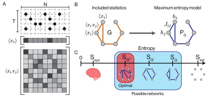
Figure 1: Identifying optimal networks of correlations. (A) Illustration of activity time series data with $N$ neurons and $T$ samples. Each point represents an active neuron within one sample. From experimental data, we can compute statistics like average activities $\langle x_{i}\rangle$ or pairwise correlations $\langle x_{i}x_{j}\rangle$ (see Materials and Methods). (B) A set of pairwise correlations $\langle x_{i}x_{j}\rangle$ defines a network $G$. The most unbiased model that matches these correlations and the averages $\langle x_{i}\rangle$ is the maximum entropy model $P_{G}$, which is equivalent to an Ising model with external fields $h_{i}$ and interactions $J_{ij}$. (C) Each set of correlations—that is, each network $G$—induces a maximum entropy $S_{G}$ that lies between the entropy of independent neurons $S_{\text{ind}}$ and the true entropy of the system $S_{\text{sys}}$ (to which we do not have access). Among possible networks $G$, the optimal one induces the minimum entropy $S_{G}$. This optimal maximum entropy model $P_{G}$ is the minimax entropy model.

The maximum entropy principle provides the unique model that matches a set of experimental statistics and nothing else, but how should we select the most important statistics to begin with? Among all networks of correlations $G$, we would like to find the one that produces the most accurate description of the system. Specifically, we can choose $G$ to maximize the log-likelihood of the model $P_{G}$, or, equivalently, minimize the KL divergence with the data $D_{\text{KL}}(P_{\text{exp}}||P_{G})$, where $P_{\text{exp}}$ is the experimental distribution over states. Due to the special form of $P_{G}$ in Eq. [1], this KL divergence simplifies to a difference in entropies,

$$D_{\text{KL}}\left(P_{\text{exp}}||P_{G}\right)=S_{G}-S_{\text{exp}}\geq 0,$$ (2)

where $S_{G}$ and $S_{\text{exp}}$ are the entropies of the model and the data, respectively (see Materials and Methods). Therefore, the optimal network $G$ (which minimizes the KL divergence) is the one that produces the maximum entropy model $P_{G}$ with the minimum entropy $S_{G}$ (Fig. 1C). This minimax entropy principle was originally proposed in the context of machine learning, but has received almost no attention in the study of biological systems Zhu et al. (1997).

In addition to providing the most accurate description of the system, the optimal network $G$ can also be viewed as containing the maximum information about system activity. When we include a network of correlations $G$ in our model, our uncertainty about the system is reduced by an amount $I_{G}=S_{\text{ind}}-S_{G}\geq 0$, where $S_{\text{ind}}$ is the entropy of independent neurons. This is precisely the amount of information that the correlations in $G$ capture about the distribution over states. Therefore, by minimizing the entropy $S_{G}$, the optimal network not only minimizes the KL divergence with the data, it also maximizes the information $I_{G}$ Lynn et al. (2023b, a).

Exact Models with Loops

While the minimax entropy principle determines the most informative correlations, which yield the most accurate description of a system, in practice we must overcome two distinct challenges. First, for each network $G$, we must compute the entropy of the maximum entropy model $S_{G}$. In general, computing the entropy exactly requires summing over all $2^{N}$ states of the system, limiting us to small systems of $N\lesssim 20$ neurons; and even approximating the entropy for larger systems is notoriously difficult Strong et al. (1998). Second, even if we can compute the entropy $S_{G}$ for a given network $G$, we still need to search over all possible networks—that is, all combinations of correlations—to choose the model with the lowest entropy. This is a combinatorial optimization problem with a search space that explodes super-exponentially with the number of neurons $N$ Korte et al. (2011).

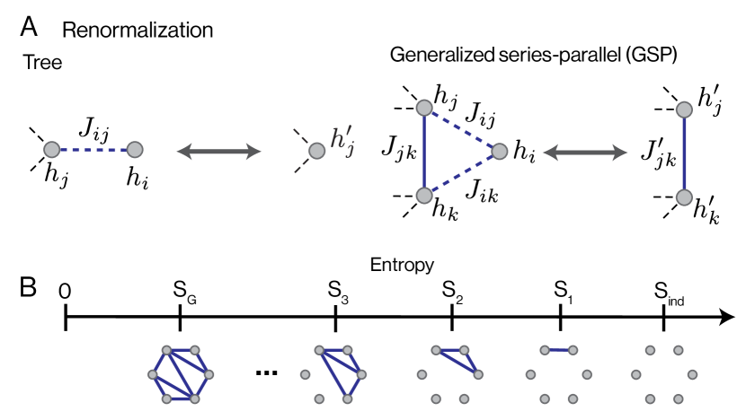
Figure 2: Exact renormalization and greedy algorithm. (A) For a model $P_{G}$ with interactions that form a tree, one can compute the partition function $Z$ (and thus all other statistics) by iteratively summing over nodes with one connection (left). We extend exact renormalization to sum over nodes with two connections (right; see Materials and Methods). This allows us to solve the maximum entropy problem exactly for a more general class of networks known as generalized series-parallel (GSP) networks. Moreover, these techniques cannot be extended further, making GSP networks the most general class of models that can be solved with exact renormalization. (B) Greedy algorithm for constructing the minimax entropy model. Beginning with an empty network (right), we iteratively connect one new neuron to two previously-connected neurons. At each step, we choose the new connections that locally minimize the entropy of the model. Once all neurons have been connected, we arrive at our minimax entropy network $G$ (left).

In statistical physics, many difficult problems become tractable if the interactions $J_{ij}$ do not contain loops Baxter (2016). Indeed, it was recently shown that the minimax entropy problem can be solved exactly and efficiently for networks $G$ without loops, known as trees Lynn et al. (2023b, a). The key insight is that the partition function $Z$ in Eq. [1] can be computed by iteratively summing over neurons $i$ with one connection (Fig. 2A). This process, known as exact renormalization Rosten (2012), is thought to be possible only if the network does not contain loops, as in one-dimensional Ising models or on Bethe lattices Baxter (2016); Nguyen et al. (2017).

Here we extend exact renormalization to a more general class of networks with loops (see Materials and Methods). In particular, rather than summing over neurons with only one connection, one can compute $Z$ by iteratively summing over neurons with two connections (Fig. 2A). This is possible for a class of networks $G$ known as generalized series-parallel (GSP) networks, which include trees, planar graphs, and series-parallel networks Duffin (1965). Moreover, this procedure cannot be extended further, making GSP networks the most general class of models that can be solved with exact renormalization (see Materials and Methods). Once $Z$ is calculated, one can then compute all of the statistics in the model by taking derivatives of the form $\langle x_{i}\rangle=\frac{\partial\log Z}{\partial h_{i}}$ and $\langle x_{i}x_{j}\rangle=\frac{\partial\log Z}{\partial J_{ij}}$. Inverting this procedure, one can begin with experimental averages $\langle x_{i}\rangle_{\text{exp}}$ and correlations $\langle x_{i}x_{j}\rangle_{\text{exp}}$ on a GSP network $G$ and compute the corresponding model parameters $h_{i}$ and $J_{ij}$ (see Materials and Methods). This solves the maximum entropy problem both exactly (that is, without approximations) and efficiently, paving the way for applications to very large systems.

Greedy Algorithm

Using the above techniques, we can construct exact maximum entropy models $P_{G}$ for a class of networks with loops. But we still need to search over all possible GSP networks $G$ to find the one that provides the best description of the system, minimizing the entropy $S_{G}$. Searching by brute force is impossible for all but the smallest of networks, so we instead decompose the search into a sequence of local optimization problems Jungnickel and Jungnickel (2005). This decomposition is made possible by the fact that any GSP network can be constructed by repeatedly connecting one new neuron $i$ to two previously connected neurons $j$ and $k$. At each step of this growth process, connecting neuron $i$ to neurons $j$ and $k$ means that we are adding the correlations $\langle x_{i}x_{j}\rangle_{\text{exp}}$ and $\langle x_{i}x_{k}\rangle_{\text{exp}}$ to the constraints in our model. Including these correlations decreases the entropy of the model by an amount

$$\Delta S_{i}=S(x_{i})+S(x_{j},x_{k})-S_{\text{pair}}(x_{i},x_{j},x_{k}),$$ (3)

where $S(\cdot)$ represents the experimental entropy, and $S_{\text{pair}}(\cdot)$ represents the entropy in our model (that is, the maximum entropy consistent with the means and pairwise correlations between $i$, $j$, and $k$; see Materials and Methods). Thus, for any GSP network $G$, we are able to exactly compute the entropy of the model $P_{G}$ by combining each of these contributions,

$$S_{G}=S_{\text{ind}}-\sum_{i}\Delta S_{i}.$$ (4)

We are now prepared to write down a greedy algorithm that constructs a locally optimal GSP network by minimizing the entropy at each step (Fig. 2B):

1. Beginning with a model of independent neurons (defined by a network with no connections), we connect the pair of neurons that results in the lowest entropy; this is the pair of neurons with the largest mutual information Lynn et al. (2023b, a).

2. We then iteratively connect a new neuron $i$ to two previously connected neurons $j$ and $k$ so as to maximize the entropy drop $\Delta S_{i}$ in Eq. [3].

3. This process continues until all neurons have been added to the network.

Using this greedy algorithm, we construct a GSP network $G$ that approximately minimizes the entropy $S_{G}$, thus capturing as much information $I_{G}$ about the system as possible. Testing on simulated networks of up to $N=10,000$ neurons, this algorithm correctly identifies over $75\%$ of the ground-truth interactions $J_{ij}$ and captures over $98\%$ of the total information $I_{G}$ in the population (see Supporting Information). Together, our renormalization procedure and greedy algorithm combine to produce an exact maximum entropy model $P_{G}$ that is optimized to provide the best description of an experimental system.

Modeling Large-scale Neural Activity

The efficiency of our minimax entropy framework gives us the opportunity to study populations of neurons at the vast scales accessible in modern experiments. Each GSP network, however, only contains $2N-3$ correlations, while the total number of pairwise correlations grows quadratically as $N(N-1)/2$. This means that as $N$ grows in large experiments, we can only include a vanishingly small fraction $\sim$$4/N$ of all the pairwise correlations in any model; and even if we fit all of these, there is still no guarantee that we can predict higher-order correlations between three or more neurons. Can such a sparse network of correlations have any hope of capturing a macroscocpic fraction of the information in the data?

To answer this question, we apply our framework to 45 recordings of $N\approx 10,000$ neurons in the mouse visual system, taken from seven different mice in previous experiments Stringer et al. (2019). The activity of each neuron is measured using two-photon calcium imaging at a rate of approximately $1.5$ Hz and binarized to reflect activity significantly above baseline (see Materials and Methods). For such large experiments, each GSP network only includes $\sim$$4/N\approx 0.04\%$ of all the correlations between pairs of neurons. For such a sparse network to have any predictive power, we need a small number of correlations to contain an unusually large amount of information $I_{G}$. From Eqs. [3-4], we see that the information contained in any GSP network $G$ can be decomposed into a sum of contributions from neuron triplets, $I_{G}=S_{\text{ind}}-S_{G}=\sum_{i}\Delta S_{i}$. Averaging across all experiments, we find a mean entropy drop of $\overline{\Delta S}=0.001$ bits; this defines the amount of information (per neuron) contained in a typical GSP network, $I_{G}/N\approx\overline{\Delta S}$. However, when we look at the full distribution of entropy drops $\Delta S$, we see that it is heavy-tailed (Fig. 3A), with some rare values that are orders of magnitude larger than average. This indicates that our minimax entropy framework may be particularly will suited for this neural data.

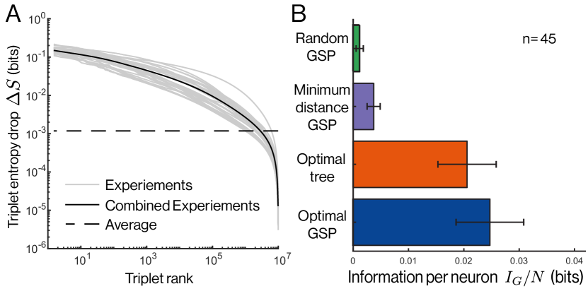
Figure 3: Information captured by different networks. (A) Distributions of entropy drops $\Delta S$ (Eq. [3]) for triplets of neurons. Grey lines represent the 45 different recordings, the black line defines the average distribution across recordings, and the dashed line illustrates the average entropy drop $\overline{\Delta S}$ across all recordings and neuron triplets. (B) Information per neuron captured by different networks of correlations. Values and error bars represent averages and standard deviations across the 45 different recordings.

Across the 45 different experiments, we find that random GSP networks only capture $I_{G}/N=0.001$ bits per neuron, as predicted by the approximation $I_{G}/N\approx\overline{\Delta S}$ (Fig. 3B). By contrast, our greedy algorithm identifies locally optimal networks that contain $I_{G}/N=0.025$ bits per neuron, over twenty times more information than a typical network. These optimized models reduce our total uncertainty about each neuron by $I_{G}/S_{\text{ind}}=10.9\%$ (compared to $I_{G}/S_{\text{ind}}=0.5\%$ for random networks), a remarkable amount considering that each network only includes two correlations per neuron. Thus, across multiple recordings, we consistently identify sparse backbones of correlations that capture large amounts of information about the neural activity.

To better understand these important correlations, we can compare against other types of networks. For example, one might suspect that neurons interact most strongly with their nearest neighbors. To test this hypothesis, we can construct GSP networks that connect the physically closest neurons in each recording; these “minimum distance” correlations only capture $I_{G}/N=0.004$ bits per neuron (Fig. 3B). Similarly, building upon past results, we can construct the most informative trees of correlations Lynn et al. (2023b, a). Across all recordings, these optimal trees capture less information than our locally optimal GSP networks (Fig. 3B). Together, these results indicate that the most important correlations include long-range connections and loops of connectivity.

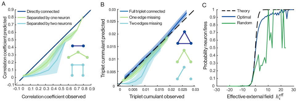
Figure 4: Predicting features of neural activity. (A) For one recording of $N=10,144$ neurons, we compare the correlation coefficients between pairs of neurons measured in data versus predicted by the minimax entropy model $P_{G}$. Different colors represent pairs of neurons separated by different distances in the network $G$, and the dashed line indicates equality. Plots are computed by binning neuron pairs along the x-axis, with lines and shaded regions representing means and standard deviations within each bin. (B) Cumulants among triplets of neurons measured in data versus predicted by our minimax entropy model. Different colors represent triplets of neurons with different numbers of pairwise correlations constrained in the model. Lines and shaded regions represent means and standard deviations within bins along the x-axis. (C) Probability of a neuron $i$ being active as a function of the effective field $h_{i}^{\text{eff}}(\bm{x})$ computed in the minimax entropy model (blue) and for a random network (green). Plots are averaged over all neurons within the population, and the dashed line represents the analytic prediction in Eq. [5].

Predicting Correlations in Neural Activity

By maximizing the information $I_{G}$, we hope to arrive at a model $P_{G}$ that can be used to predict structure in the neural activity. In general, making exact predictions in the Ising model (Eq. [1]) is infeasible, and approximations require time-consuming Monte Carlo simulations. Here, by generalizing the famous Bethe solution for trees Baxter (2016), we derive exact and efficient model predictions for our class of GSP networks (see Materials and Methods).

In Fig. 4A, we compare the experimental correlation coefficients between neurons with the values predicted by our minimax entropy model $P_{G}$. We focus on a single population of $N=10,144$ neurons recorded while the mouse is exposed to a sequence of natural images Stringer et al. (2019). For pairs of neurons $i$ and $j$ connected in the network $G$, the model exactly matches the observed correlations, as desired. For neurons separated by one intermediate neuron, the model still provides reasonable predictions, even for very strong correlations. This demonstrates that some pairwise correlations can be explained as arising indirectly through shared correlations with a third neuron. As we increase the distance between neurons in the network, the model predictions become less accurate, indicating that indirect interactions via two or more intermediate neurons are not sufficient to explain the observed correlations.

In addition to pairwise statistics, we can also investigate higher-order correlations among groups of neurons. In Fig. 4B, we compare the triplet cumulants $\langle(x_{i}-\langle x_{i}\rangle)(x_{j}-\langle x_{j}\rangle)(x_{k}-\langle x_{k}\rangle)\rangle$ predicted by our model $P_{G}$ with those measured in experiment. For triplets that are fully connected in $G$—such that all three pairwise correlations are constrained in $P_{G}$—the model accurately predicts the triplet correlations within experimental errors. Even with one correlation missing, our model still accurately predicts the triplet cumulants. By contrast, a random set of pairwise correlations (that is, a typical network $G$) provides almost no predictive power about these higher-order correlations (see Supporting Information).

At the level of individual cells, each model $P_{G}$ makes a clear prediction for the response of neuron $i$ to the state of the rest of the population,

$$P_{G}(x_{i}=1\,|\,\bm{x})=\big{(}1+\exp(-h_{i}^{\text{eff}}(\bm{x}))\big{)}^{-1},$$ (5)

where $h_{i}^{\text{eff}}(\bm{x})=h_{i}+\sum_{j\in G_{i}}J_{ij}x_{j}$ is the effective field on neuron $i$ and $G_{i}$ denotes the neighbors of $i$ in $G$ Lynn et al. (2023b, a); Meshulam et al. (2023). In Fig. 4C, we see that a random set of correlations is insufficient to predict the responses of individual neurons. Meanwhile, our optimized GSP network exhibits good agreement with data across a wide range of spike probabilities. Together, the results of Fig. 4 demonstrate that our minimax entropy framework, despite only including two correlations per neuron, is capable of predicting key features of collective neural activity. This is only possible because we select the most informative correlations in the population.

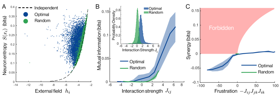
Figure 5: Structure of optimal model. (A) Neuron entropies $S(x_{i})$ versus external fields $h_{i}$ computed in the optimal model (blue) and a random network (green). Dashed line illustrates the independent prediction. (B) Mutual information between neurons versus the inferred interaction $J_{ij}$ for different models. (B, Inset) Distribution of inferred interactions $J_{ij}$ for the optimal model and a random network. (C) Synergy versus frustration $-J_{ij}J_{jk}J_{ki}$ among triplets of neurons for different models. The red region cannot be attained by any Ising triplet.

Structure of Minimax Entropy Model

Given a GSP network of correlations $G$, we provide the tools to exactly infer the maximum model $P_{G}$ in Eq. [1] (see Materials and Methods), which is equivalent to an Ising model with binary states $x_{i}\in\{0,1\}$. Leveraging this connection to statistical physics, we can investigate the different types of models produced by different networks $G$. For example, each external field $h_{i}$ represents the individual bias for neuron $i$ towards activity or silence. For an independent neuron, this field precisely defines the average activity $\langle x_{i}\rangle=1/(1+e^{-h_{i}})$ and therefore the independent entropy $S(x_{i})$. For a random network $G$, because the correlations are so weak, the entropy of each neuron closely follows this independent prediction (Fig. 5A). Meanwhile, the minimax entropy framework identifies a strong network of correlations, leading to neuron entropies $S(x_{i})$ that significantly differ from independence.

In each model, the interactions $J_{ij}$ represent the influence of neuron $i$ to induce activity ($J_{ij}>0$) or silence ($J_{ij}<0$) in neuron $j$, and vice versa. For a random network, these interactions are evenly split between positive and negative (Fig. 5B, Inset), yielding a description that is akin to the Sherrington-Kirkpatrick model of a spin glass Sherrington and Kirkpatrick (1975). The most informative correlations, by contrast, produce almost exclusively positive interactions. This makes the minimax entropy model $P_{G}$ similar to an Ising ferromagnet, in which positive interactions can build upon one another to generate large-scale order and long-range correlations Newell and Montroll (1953); Brush (1967).

Using our exact solution to the maximum entropy problem, we can gain insight into how the interactions $J_{ij}$ relate to the information $I_{G}$ that a network captures about neural activity. For a GSP network $G$, we derive the following decomposition of the information into non-negative components (see Materials and Methods),

$$I_{G}=\sum_{(ij)\in G}I(x_{i},x_{j})+\sum_{(ijk)\in G}\text{Syn}(x_{i},x_{j},x_{k}),$$ (6)

where $I(x_{i},x_{j})=S(x_{i})+S(x_{j})-S(x_{i},x_{j})$ is the mutual information between neurons $i$ and $j$, and the second sum runs over all triplets $(ijk)$ that form a triangle in $G$. Inside the final sum is the synergy $\text{Syn}(x_{i},x_{j},x_{k})$ (see Materials and Methods), which represents the amount of information that two neurons contain about a third above and beyond their mutual information Schneidman et al. (2003a, b). This decomposition tells us that optimal GSP network $G$ should focus on pairs of neurons with large mutual informations and triplets with large synergies.

The interactions $J_{ij}$ in our optimized network, in addition to being mostly positive, are also much stronger than those in the random network. In Fig. 5B, we see that these strongly positive interactions produce pairs of neurons with large mutual informations, as desired. For comparison, synergy increases if the interactions between neurons present competing influences Schneidman et al. (2003a, b); in the Ising model, competing interactions give rise to frustration, which we can quantify using the product $-J_{ij}J_{jk}J_{ki}$. We note that synergy and frustration can only arise in networks with loops, and therefore cannot be studied using previous methods on trees Lynn et al. (2023b, a). In GSP networks, we find that positive synergy can only be achieved by frustrated triplets (Fig. 5C). However, in our minimax entropy model, we find that most triplets have negative synergy, such that neurons contain redundant information about one another (Fig. 5C). These results demonstrate that to maximize the information $I_{G}$ in this neural population, the optimal model focuses on pairs of neurons with large mutual informations (underpinned by strongly positive interactions), even at the expense of synergistic information.

Effects of Visual Stimulation

In the visual cortex, neural activity is strongly driven by details in the visual world Stringer et al. (2019); Gilbert and Li (2013). Yet these patterns of activity are also shaped by recurrent connections, which form feedback loops of interactions that do not change from one stimulus to another Ko et al. (2013); Hofer et al. (2011); Smith and Kohn (2008). This raises a clear question: Do the most important correlations between neurons remain consistent across stimuli, or do they depend crucially on the visual scene?

Out of the 45 different recordings of $N\approx 10,000$ neurons (Fig. 3), 26 correspond to populations that were recorded twice—once in response to visual stimuli (either natural images or drifting gratings) and once during spontaneous activity (with a grey or black screen). Across triplets of neurons, we find almost identical distributions of entropy drops $\Delta S$ (Eq. [3]) between responding and spontaneous activity (Fig. 6A). This suggests that for any GSP network $G$, the amount of information contained in the correlations $I_{G}=\sum_{i}\Delta S_{i}$ will be consistent across the two conditions. Indeed, for random networks, we find that the typical information per neuron $I_{G}/N\approx\overline{\Delta S}$ does not vary significantly between conditions (see Supporting Information). However, focusing on the networks identified by our minimax entropy framework, the most important correlations in the populations contain $30\%$ more information when responding to visual stimuli than in spontaneous activity (Fig. 6B). This means that, for the same neurons and the same number of correlations, one can achieve a better description of the neural activity when the population is driven by visual cues.

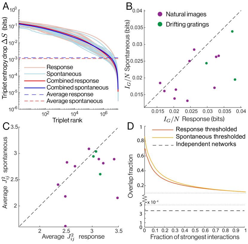
Figure 6: Effects of visual stimulation on optimal correlations. (A) Distributions of entropy drops $\Delta S$ (Eq. [3]) for triplets of neurons during visual stimulation (red) and spontaneous activity (blue). Dark lines define the average distributions for each stimulus condition, and the dashed lines illustrate the average entropy drops $\overline{\Delta S}$. (B) Information per neuron $I_{G}/N$ captured by the optimal networks $G$ for visual responses and spontaneous activity. Each point represents a unique neural population, colors indicate the type of visual stimulus, and the dashed line defines equality. (C) Average squared interaction strengths $J_{ij}^{2}$ in the minimax entropy models $P_{G}$ fit to the same populations during visual responses or spontaneous activity. (D) Fractional overlap between optimal networks during visual responses and spontaneous activity. For each population, we either threshold the visual response network (red) or the spontaneous network (yellow) based on the strongest inferred interactions $J_{ij}$ and leave the other network fixed to compute the overlap. Two independent networks would have an overlap of $\sim$$4/N$, which for $N\approx 10,000$ is $0.04\%$ (dashed line).

To understand this difference in information, we can study the structures of the optimal models $P_{G}$. For responses to visual stimuli, we find that the inferred interactions between neurons $J_{ij}$ are stronger than for spontaneous activity (Fig. 6C). This increase in interaction strength corresponds to an increase in the mutual informations between neurons, as seen previously (Fig. 5B). Yet despite these differences in interaction strengths, the optimal networks themselves remain remarkably consistent between conditions. For two independent networks with $N=10,000$ nodes and $2N$ connections, we expect a fractional overlap of $\sim$$4/N=0.04\%$. By contrast, the most informative correlations within each population exhibit an overlap of $12\%$ between responding and spontaneous activity, over two orders of magnitude more than independent networks (Fig. 6D). This overlap grows even larger as we focus on stronger interactions $J_{ij}$ within the optimal networks (Fig. 6D), reaching $70-85\%$ for the strongest interactions Hoshal et al. (2024).

Together, these results demonstrate that (i) the information contained in correlations increases when responding to visual stimuli (Fig. 6B); but (ii) the networks formed by these correlations remain strikingly consistent from spontaneous to stimulated activity (Fig. 6D). In turn, this suggests that the most important correlations in the visual system may driven by actual interactions between neurons—thus remaining consistent across stimuli—but that these correlations are amplified when responding to visual cues.

Discussion

As experimental techniques advance, enabling simultaneous recordings of larger and larger populations of neurons Urai et al. (2022); Gauthier and Tank (2018); Stringer et al. (2019); Steinmetz et al. (2021); Demas et al. (2021); Chung et al. (2019); Manley et al. (2024), we face new challenges in extracting meaningful statistical structure at vast scales. The primary difficulty lies in constructing quantitative models that can be used to predict the probabilities of high-dimensional patterns of activity. While recent techniques from statistical physics have solved this problem in models without loops of connectivity Lynn et al. (2023b, a), the cortex is known to exhibit complex circuits of recurrent connections between neurons Bullmore and Sporns (2009); Lin et al. (2024); Lynn et al. (2024); Bullmore and Sporns (2012); Wang (2010); Lynn and Bassett (2019).

Here, for a class of models with loops, we present an exact solution to the maximum entropy problem that scales to very large systems. This solution gives us direct access to information-theoretic quantities like the entropy of the model and the amount of information that it captures about the system, which are usually inaccessible at large scales (Fig. 1). In turn, this allows us to search for the model that provides the best description of the data, and we present a locally optimal algorithm for executing this search (Fig. 2). The end result is a framework for (i) identifying the most important correlations within large neuronal populations and (ii) using these correlations to make exact predictions about collective activity.

We apply our methods to 45 recordings of approximately $10,000$ neurons in the mouse visual cortex Stringer et al. (2019). In each recording, we identify optimal correlations that contain over twenty times more information than typical networks (Fig. 3). This information allows us to quantitatively predict additional correlations between pairs and triplets of neurons that were not included in the model (Fig. 4). Notably, the optimal correlations in a population capture more information during visual stimulation than spontaneous activity; however, the networks formed by these correlations remain strikingly consistent, hinting at a common underlying neural circuitry (Fig. 6).

Broadly, we present a framework—based on the little-known minimax entropy principle Baxter (2016); Lynn et al. (2023b, a)—for constructing optimized statistical models of the large populations becoming accessible in modern experiments. These methods are general, applying to any system with binary data. This opens the door for future investigations into collective neural activity in other systems, species, and imaging modalities Lynn and Bassett (2019); Tkačik et al. (2015); Marre et al. (2009); Meshulam et al. (2023); Lynn et al. (2023b, a); Ashourvan et al. (2021); Rosch et al. (2024); Urai et al. (2022); Gauthier and Tank (2018); Stringer et al. (2019); Steinmetz et al. (2021); Demas et al. (2021); Chung et al. (2019); Manley et al. (2024). One can also use the same techniques to study collective behaviors in other complex living systems, such as genetic interactions, chromatin structure, and animal behaviors Lynn et al. (2019); Shi and Thirumalai (2023); Messelink et al. (2021); Lezon et al. (2006); Dixit (2013); Weigt et al. (2009); Marks et al. (2011); Bialek et al. (2012, 2014); Mora et al. (2010). Finally, our exact maximum entropy solution provides the foundation for the future development of improved approximate models, for example based on mean-field techniques and cluster expansions Yedidia et al. (2005); Tanaka (2000); Cocco and Monasson (2011, 2012). In this way, our minimax entropy framework provides a principled starting point for statistical models (with loops) of large-scale neural activity.

Materials and Methods

Data

The data consists of calcium imaging recordings of populations of $N=10506\pm 1737$ (mean $\pm$ standard deviation) from the mouse visual system at a sampling rate of about 1.5 Hz, measured in previous experiments Stringer et al. (2019). We study 45 recordings of 7 separate mice who were free to run on an air-floating ball as images were presented on three computer screens. Stimuli included natural images, distorted natural images, drifting gratings, and grey screens (to measure spontaneous activity). These stimuli were presented to the mice on average $T=4570\pm 1486$ times during each recording, and the sampling of neural activity across all neurons aligns with the stimulus presentations. The recordings can be broadly divided into two groups: responses to stimuli and spontaneous activity. There are 13 instances of neuronal populations being recorded both during spontaneous activity and while responding to stimuli (10 for natural images and 3 for drifting gratings). These pairs of recordings capture the same sets of neurons in the same mice under different stimulus conditions.

The activity of each neuron was binarized into active ($x_{i}=1$) or silent ($x_{i}=0$) at each moment of time based on whether or not its calcium trace reached two standard deviations above its mean activity. The collective activity is then defined by the binary vector $\bm{x}=\{x_{i}\}$. Due to the large number of neurons, there are pairs of neurons that never fire together during a recording. When computing experimental averages, we correct for this by adding one pseudo-count, such that the experimental statistics are given by

$$\left<x_{i}\right> =\frac{1}{1+T}\left(1+\sum_{t=1}^{T}x_{i}(t)\right),$$ (7)

$$\left<x_{i}x_{j}\right> =\frac{1}{1+T}\left(1+\sum_{t=1}^{T}x_{i}(t)x_{j}(t)\right),$$ (8)

where $x_{i}(t)$ defines the activity of neuron $i$ at time $t$.

Maximum Entropy Principle

The maximum entropy principle determines the least biased model that matches a specified set of statistical constraints Jaynes (1957); Thomas M. Cover and Joy A. Thomas (2006). Here, we focus on a model constrained to match the empirical averages of neural activity $\langle x_{i}\rangle$ and a subset of the pairwise correlations $\langle x_{i}x_{j}\rangle$ that lie on a network $G$. The maximum entropy model consistent with these constraints takes the form of an Ising model with interactions that lie on the network $G$ (Eq. [1]). For an all-to-all network $G$, one arrives at the pairwise maximum entropy model, which has provided key insights into the collective behavior of smaller populations of up to $N\sim 100$ neurons Schneidman et al. (2006); Nguyen et al. (2017); Meshulam et al. (2017); Tkačik et al. (2015); Meshulam et al. (2023).

Partition Function

For an Ising model with interactions that lie on a GSP network $G$ [Eq. (1)], we provide an exact solution for the statistics $\langle x_{i}\rangle$ and $\langle x_{i}x_{j}\rangle$ as functions of the parameters $h_{i}$ and $J_{ij}$. As a first step, we compute the partition function $Z$. Introducing a zero-point energy $f=0$, which will soon become useful, the Boltzmann distribution takes the form

$$P_{G}(\bm{x})=\frac{1}{Z}\text{exp}\Bigg{[}\sum_{(ij)\in G}J_{ij}x_{i}x_{j}+\sum_{i}h_{i}x_{i}+f\Bigg{]}.$$ (9)

To compute the partition function,

$$Z=\sum_{\bm{x}}\text{exp}\Bigg{[}\sum_{(ij)\in G}J_{ij}x_{i}x_{j}+\sum_{i}h_{i}x_{i}+f\Bigg{]},$$ (10)

we start by summing over one variable. Our goal is to find a new system of $N-1$ variables with the same partition function $Z$. If we can repeat this process until no variables remain, then computing $Z$ will be trivial.

We label the nodes $i=1,\ldots,N$ based on the order that they are removed (or summed over), and we let, $J^{(i)}_{jk}$, $h^{(i)}_{i}$, and $f^{(i)}$ denote the updated parameters at step $i$. Consider summing over a variable $i$ with only two connections in the network, say to variables $j$ and $k$, which themselves are connected (such that $J_{jk}\neq 0$). In GSP networks, such a node $i$ is always guaranteed to exist. To keep the partition function fixed, the new system with $i$ removed must satisfy the equations

$$e^{J_{jk}^{(i)}x_{j}x_{k}+h_{j}^{(i)}x_{j}+h_{k}^{(i)}x_{k}+f^{(i)}}\big{(}e^{J_{ij}^{(i)}x_{j}+J_{ik}^{(i)}x_{k}+h^{(i)}_{i}}+1\big{)}=\\ e^{J_{jk}^{(i+1)}x_{j}x_{k}+h_{j}^{(i+1)}x_{j}+h_{k}^{(i+1)}x_{k}+f^{(i+1)}}.$$ (11)

This is a system of four equations (one for each value of $x_{j}$ and $x_{k}$), which we can solve for the new parameters

$$f^{(i+1)} =f^{(i)}+\ln\left(e^{h_{i}^{(i)}}+1\right),$$ (12)

$$h_{j}^{(i+1)} =h_{j}^{(i)}-\ln\left(e^{h_{i}^{(i)}}+1\right)+\ln\left(e^{J_{ij}^{(i)}+h_{i}^{(i)}}+1\right),$$ (13)

$$h_{k}^{(i+1)} =h_{k}^{(i)}-\ln\left(e^{h_{i}^{(i)}}+1\right)+\ln\left(e^{J_{ik}^{(i)}+h_{i}^{(i)}}+1\right),$$ (14)

$$J_{jk}^{(i+1)} =J_{jk}^{(i)}+\ln\left(e^{h_{i}^{(i)}}+1\right)-\ln\left(e^{J_{ij}^{(i)}+h_{i}^{(i)}}+1\right)$$ (15)

$$-\ln\left(e^{J_{ik}^{(i)}+h_{i}^{(i)}}+1\right)+\ln\left(e^{J_{ij}^{(i)}+J_{ik}^{(i)}+h_{i}^{(i)}}+1\right).$$

After repeating the above procedure $N$ times, we have summed over all nodes, and we are left with a single parameter $\mathcal{F}=f^{(N+1)}$. This is the negative free energy, and the partition function is given by

$$Z=e^{\mathcal{F}}.$$ (16)

At each step, we have assumed that we can find a node $i$ with only two connections to nodes $j$ and $k$ that are themselves connected. After removing $i$, we must find another such node to repeat the calculation. The class of networks for which this process can continue down to a final root node are precisely the set of GSP networks Korneyenko (1994). Moreover, we note that this is the furthest we can push this technique. Attempting to remove any node with three neighbors would lead to an overdetermined system of 8 equations and 7 parameters. In this case, one would need to introduce an additional triplet interaction between the tree neighbors, and we would diverge from the realm of Ising models. We therefore establish that GSP networks are the most general class of networks that can be solved through exact renormalization.

Average Activities and Correlations

To compute statistics, we take derivatives of the partition function,

$$\langle x_{i}\rangle =\frac{d\ln Z}{dh_{i}}=\frac{d\mathcal{F}}{dh_{i}},$$ (17)

$$\langle x_{i}x_{j}\rangle =\frac{d\ln Z}{dJ_{ij}}=\frac{d\mathcal{F}}{dJ_{ij}},$$ (18)

where $\frac{d}{dh_{i}}$ and $\frac{d}{dJ_{ij}}$ represent total derivatives, which account for indirect dependencies via Eqs. [12]-[15]. Since $\frac{d\mathcal{F}}{df^{(i+1)}}=1$ and $\frac{dh_{i}^{(i)}}{dh_{i}}=1$, the above procedure yields

$$\langle x_{i}\rangle=\frac{\partial f^{(i+1)}}{\partial h^{(i)}_{i}}+\frac{d\mathcal{F}}{dh^{(i+1)}_{j}}\frac{\partial h^{(i+1)}_{j}}{\partial h^{(i)}_{i}}+\frac{d\mathcal{F}}{dh^{(i+1)}_{k}}\frac{\partial h^{(i+1)}_{k}}{\partial h^{(i)}_{i}}\\ +\frac{d\mathcal{F}}{dJ^{(i+1)}_{jk}}\frac{\partial J^{(i+1)}_{jk}}{\partial h^{(i)}_{i}}.$$ (19)

Noticing that

$$\frac{d\mathcal{F}}{dh^{(i+1)}_{j}} =\frac{d\mathcal{F}}{dh_{j}}=\langle x_{j}\rangle,$$ (20)

$$\frac{d\mathcal{F}}{dh^{(i+1)}_{k}} =\frac{d\mathcal{F}}{dh_{k}}=\langle x_{k}\rangle,$$ (21)

$$\frac{d\mathcal{F}}{dJ^{(i+1)}_{jk}} =\frac{d\mathcal{F}}{dJ_{jk}}=\langle x_{j}x_{k}\rangle,$$ (22)

and taking derivatives of Eqs. [12]-[15], we have

$$\left<x_{i}\right>=\frac{1-\left<x_{j}\right>-\left<x_{k}\right>+\left<x_{j}x_{k}\right>}{1+e^{-h^{(i)}_{i}}}+\frac{\left<x_{j}\right>-\left<x_{j}x_{k}\right>}{1+e^{-J^{(i)}_{ij}-h^{(i)}_{i}}}\\ +\frac{\left<x_{k}\right>-\left<x_{j}x_{k}\right>}{1+e^{-J^{(i)}_{ik}-h^{(i)}_{i}}}+\frac{\left<x_{j}x_{k}\right>}{1+e^{-J^{(i)}_{ij}-J^{(i)}_{ik}-h^{(i)}_{i}}}.$$ (23)

The correlations follow analogously,

$$\left<x_{i}x_{j}\right>=\frac{\left<x_{j}\right>-\left<x_{j}x_{k}\right>}{1+e^{-J^{(i)}_{ij}-h^{(i)}_{i}}}+\frac{\left<x_{j}x_{k}\right>}{1+e^{-J^{(i)}_{ij}-J^{(i)}_{ik}-h^{(i)}_{i}}},$$ (24)

$$\left<x_{i}x_{k}\right>=\frac{\left<x_{k}\right>-\left<x_{j}x_{k}\right>}{1+e^{-J^{(i)}_{ik}-h^{(i)}_{i}}}+\frac{\left<x_{j}x_{k}\right>}{1+e^{-J^{(i)}_{ij}-J^{(i)}_{ik}-h^{(i)}_{i}}}.$$ (25)

Thus, by iterating through the nodes in the opposite order from which they were summed over to compute $Z$, we can compute the average activities $\langle x_{i}\rangle$ and correlations $\langle x_{i}x_{j}\rangle$ for pairs $(ij)\in G$. For the correlations $\langle x_{i}x_{j}\rangle$ that are not in the network (that is, for $(ij)\not\in G$), see Supporting Information.

Maximum Entropy Solution

We have solved the “forward” problem for an Ising model on a GSP network. Now we seek to solve the “inverse” (or maximum entropy) problem for the parameters $h_{i}$ and $J_{ij}$ as functions of the observed statistics $\langle x_{i}\rangle$ and $\langle x_{i}x_{j}\rangle$. In practice, this amounts to inverting Eqs. [23]-[25]. We start with the last node in the decimation order $i=N$ and calculate its external field from its empirical average as

$$h_{N}^{(N)}=\ln\left(\frac{\langle x_{N}\rangle}{1-\langle x_{N}\rangle}\right).$$ (26)

Next, we connect node $i=N-1$ to node $i=N$, yielding the parameters

$$h_{N-1}^{(N-1)}=\ln\left(\frac{\langle x_{N}\rangle-\langle x_{N,N-1}\rangle}{1+\langle x_{N,N-1}\rangle-\langle x_{N}\rangle-\langle x_{N-1}\rangle}\right),$$ (27)

$$J_{N,N-1}^{(N-1)}\ln\left(\frac{\langle x_{N,N-1}\rangle}{\langle x_{N}\rangle-\langle x_{N,N-1}\rangle}\right)-h_{N-1}^{(N-1)}.$$ (28)

We must also update the external field on node $i=N$,

$$h_{N}^{(N-1)}=h_{N}^{(N)}+\ln\left(e^{h_{N-1}^{(N-1)}}+1\right)\\ -\ln\left(e^{h_{N-1}^{(N-1)}+J_{N,N-1}^{(N-1)}}+1\right).$$ (29)

For the remaining nodes $i=N-2,\ldots,1$, we must invert Eqs. [23]-[25] numerically to calculate $h_{i}^{(i)}$, $J_{ij}^{(i)}$,$J_{ik}^{(i)}$ in terms of $\langle x_{i}\rangle$, $\langle x_{i}x_{j}\rangle$, and $\langle x_{i},x_{k}\rangle$, where $j$ and $k$ are the parents of $i$. We can then use Eqs. [12]-[15] to update $h^{(i)}_{j}$, $h^{(i)}_{k}$, $J^{(i)}_{jk}$. This process continues until all nodes have been added to the network, and we arrive at the solution $h_{i}=h_{i}^{(1)}$ and $J_{ij}=J_{ij}^{(1)}$.

Minimax Entropy

For a given network $G$, the difference between the maximum entropy distribution $P_{G}$ and the experimental distribution $P_{\text{exp}}$ is quantified by the Kullback–Leibler (KL) divergence,

$$D_{\text{KL}}(P_{\text{exp}}||P_{G})=\left\langle\ln\left(\frac{P_{\text{exp}}(\bm{x})}{P_{G}(\bm{x})}\right)\right\rangle_{\text{exp}}$$ (30)

$$=-S_{\text{exp}}+\ln(Z)-\sum_{(ij)\in G}J_{ij}\left<x_{i}x_{j}\right>_{\text{exp}}-\sum_{i}h_{i}\left<x_{i}\right>_{\text{exp}}$$ (31)

$$=-S_{\text{exp}}+\ln(Z)-\sum_{(ij)\in G}J_{ij}\left<x_{i}x_{j}\right>-\sum_{i}h_{i}\left<x_{i}\right>$$ (32)

$$=S_{G}-S_{\text{exp}},$$ (33)

where the penultimate equality follows from the maximum entropy constraints $\langle x_{i}\rangle=\langle x_{i}\rangle_{\text{exp}}$ and $\langle x_{i}x_{j}\rangle=\langle x_{i}x_{j}\rangle_{\text{exp}}$. The equation above tells us that the optimal network $G$, which minimizes the KL divergence from the data, is the one that minimizes the entropy $S_{G}$ of the maximum entropy model. This is the minimax entropy principle, which was discovered over 20 years ago Zhu et al. (1997), but remains largely unexplored in the study of complex living systems Lynn et al. (2023a, b).

Greedy Algorithm

Directly searching over all possible GSP networks is computationally intractable. Instead, we will take a greedy approach to minimizing entropy. As discussed above, the class of GSP networks is the set of networks that you can grow by iteratively adding a new node and connecting it to two existing nodes that are already connected (Fig. 2B). This definition leads directly to a greedy algorithm for constructing the optimal network: At each step of the network construction, we should connect a new node $i$ to two existing nodes $j$ and $k$ (that are already connected) so as to minimize the entropy $S_{G}$.

To implement this greedy algorithm, we need to compute the drop in entropy from connecting a new node $i$ to two existing nodes $j$ and $k$; this is precisely the drop in entropy from fitting the correlations $\langle x_{i}x_{j}\rangle$ and $\langle x_{i}x_{k}\rangle$ in the maximum entropy model. Before connecting $i$ in the network, the distribution over states factorizes,

$$P_{G}(\bm{x})=P_{G}(x_{i})P_{G}(\bm{x}_{-i}),$$ (34)

where $\bm{x}_{-i}$ denotes the states of all variables other than $i$. Since $P_{G}$ matches the average $\langle x_{i}\rangle$, we note that $P_{G}(x_{i})$ is the same as the experimental marginal $P(x_{i})$. After connecting $i$ to $j$ and $k$, we arrive at a new network $G^{\prime}$ with a distribution of the form

$$P_{G^{\prime}}(\bm{x})=P_{G^{\prime}}(x_{i}|x_{j},x_{k})P_{G^{\prime}}(\bm{x}_{-i}).$$ (35)

From our decimation procedure above, we know that $P_{G^{\prime}}(\bm{x}_{-i})=\sum_{x_{i}}P_{G^{\prime}}(\bm{x})=P_{G}(\bm{x}_{-i})$. The drop in entropy thus reduces to

$$\Delta S_{i} =S_{G}-S_{G^{\prime}}$$ (36)

$$=S(x_{i})+S_{G}(\bm{x}_{-i})-S_{G^{\prime}}(x_{i}|x_{j},x_{k})-S_{G}(\bm{x}_{-i})$$ (37)

$$=S(x_{i})+S(x_{i},x_{j})-S_{\text{pair}}(x_{i},x_{j},x_{k}),$$ (38)

where $S(\cdot)$ denotes the experimental entropy and $S_{\text{pair}}(\cdot)$ represents the entropy of the maximum entropy model that is consistent with the averages and all pairwise correlations between variables.

We have arrived at our greedy algorithm. At each step, we consider all combinations of new nodes $i$ and pairs $j$ and $k$ that are already connected in the network. For each triplet, we compute the entropy drop in Eq. [38], and for the largest drop, we connect $i$ to $j$ and $k$. We then repeat this process until all nodes have been connected in the network. By minimizing the entropy $S_{G}$ at each step, this greedy algorithm provides a locally optimal solution to the minimax entropy problem (Fig. 2).

Decomposing Information

Finally, we derive a decomposition of the information contained within a GSP network of correlations $G$. As discussed above, the information contained in any network of correlations is the drop in entropy $I_{G}=S_{\text{ind}}-S_{G}$, where $S_{G}$ is the entropy of the maximum entropy model $P_{G}$. For a GSP network $G$, we showed in the previous section that this information can be decomposed into a sequence of entropy drops

$$I_{G}=\sum_{i}\Delta S_{i}=\sum_{i}\Big{(}S(x_{i})+S(x_{i},x_{j})-S_{\text{pair}}(x_{i},x_{j},x_{k})\Big{)},$$ (39)

where $j$ and $k$ are the parents of $i$ in the network construction.

The decomposition in Eq. [39] depends on the order in which we add nodes to the network during construction. We will now derive a new decomposition that does not depend on this choice of order. To begin, we introduce a new quantity known as the synergy,

$$\text{Syn}(x_{i},x_{j},x_{k})=S(x_{i})+S(x_{j})+S(x_{k})-S_{\text{pair}}(x_{i},x_{j},x_{k})\\ -I(x_{i},x_{j})-I(x_{i},x_{k})-I(x_{j},x_{k}).$$ (40)

The synergy represents the amount of information that two variables contain about a third beyond their pairwise dependencies Brenner et al. (2000); Schneidman et al. (2003b). We note that the above synergy is computed in the model $P_{G}$, not the experimental distribution $P_{\text{exp}}$. We also note that the synergy is symmetric under permutations of $x_{i}$, $x_{j}$, and $x_{k}$. Substituting into Eq. [39], we have

$$I_{G}=\sum_{i}\text{Syn}(x_{i},x_{j},x_{k})+I(x_{i},x_{j})+I(x_{i},x_{k}).$$ (41)

When a new variable $i$ is added to the network, we create two new edges (connecting $i$ to $j$ and $k$) and one new triangle (among $i$, $j$, and $k$). We therefore see that the above sum can be rewritten as a sum over network motifs: edges and triangles. This gives us a decomposition of the information that does not depend on our choice of node order in the network construction,

$$I_{G}=\sum_{(ij)\in G}I(x_{i},x_{j})+\sum_{(ijk)\in G}\text{Syn}(x_{i},x_{j},x_{k}),$$ (42)

where the first sum runs over all edges in $G$, and the second sum runs over all fully-connected triplets of neurons (triangles) in $G$. This decomposition for GSP networks generalizes previous decompositions of the information contained in trees of correlations, or networks without loops Lynn et al. (2023b, a).

References

- Wiener (1966) Norbert Wiener, Nonlinear Problems In Random Theory (MIT Press, Cambridge MA, 1966).
- Cooper (1973) L. N. Cooper, “A Possible Organization of Animal Memory and Learning1,” in Collective Properties of Physical Systems, edited by BENGT Lundqvist and STIG Lundqvist (Academic Press, 1973) pp. 252–264.
- Little (1996) W. A. Little, “The Existence of Persistent States in the Brain,” in From High-Temperature Superconductivity to Microminiature Refrigeration, edited by Blas Cabrera, H. Gutfreund, and Vladimir Kresin (Springer US, Boston, MA, 1996) pp. 145–164.
- Hopfield (1982) J J Hopfield, “Neural networks and physical systems with emergent collective computational abilities.” Proceedings of the National Academy of Sciences 79, 2554–2558 (1982).
- Amit (1989) Daniel J. Amit, Modeling Brain Function: The World of Attractor Neural Networks (Cambridge University Press, Cambridge, 1989).
- Hertz et al. (1991) John Hertz, Anders Krogh, and Richard G Palmer, Introduction to the Theory of Neural Computation (Addison-Wesley, Redwood City, 1991).
- Schneidman et al. (2006) Elad Schneidman, Michael J. Berry, Ronen Segev, and William Bialek, “Weak pairwise correlations imply strongly correlated network states in a neural population,” Nature 440, 1007–1012 (2006).
- Nguyen et al. (2017) H. Chau Nguyen, Riccardo Zecchina, and Johannes Berg, “Inverse statistical problems: from the inverse Ising problem to data science,” Advances in Physics 66, 197–261 (2017).
- Meshulam et al. (2017) Leenoy Meshulam, Jeffrey L. Gauthier, Carlos D. Brody, David W. Tank, and William Bialek, “Collective Behavior of Place and Non-place Neurons in the Hippocampal Network,” Neuron 96, 1178–1191.e4 (2017).
- Tkačik et al. (2015) Gašper Tkačik, Thierry Mora, Olivier Marre, Dario Amodei, Stephanie E. Palmer, Michael J. Berry, and William Bialek, “Thermodynamics and signatures of criticality in a network of neurons,” Proceedings of the National Academy of Sciences 112, 11508–11513 (2015).
- Marre et al. (2009) Olivier Marre, Sami El Boustani, Yves Fregnac, and Alain Destexhe, “Prediction of spatiotemporal patterns of neural activity from pairwise correlations,” Phys. Rev. Lett. 102, 138101 (2009).
- Lynn et al. (2023a) Christopher W. Lynn, Qiwei Yu, Rich Pang, William Bialek, and Stephanie E. Palmer, “Exactly solvable statistical physics models for large neuronal populations,” ArXiv , arXiv:2310.10860v1 (2023a).
- Lynn et al. (2023b) Christopher W. Lynn, Qiwei Yu, Rich Pang, Stephanie E. Palmer, and William Bialek, “Exact minimax entropy models of large-scale neuronal activity,” (2023b).
- Meshulam et al. (2023) Leenoy Meshulam, Jeffrey L. Gauthier, Carlos D. Brody, David W. Tank, and William Bialek, “Successes and failures of simple statistical physics models for a network of real neurons,” (2023).
- Ashourvan et al. (2021) Arian Ashourvan, Preya Shah, Adam Pines, Shi Gu, Christopher W Lynn, Danielle S Bassett, Kathryn A Davis, and Brian Litt, “Pairwise maximum entropy model explains the role of white matter structure in shaping emergent co-activation states,” Commun. Biol. 4, 210 (2021).
- Rosch et al. (2024) Richard E Rosch, Dominic RW Burrows, Christopher W Lynn, and Arian Ashourvan, “Spontaneous brain activity emerges from pairwise interactions in the larval zebrafish brain,” Phys. Rev. X 14, 031050 (2024).
- Urai et al. (2022) Anne E Urai, Brent Doiron, Andrew M Leifer, and Anne K Churchland, “Large-scale neural recordings call for new insights to link brain and behavior,” Nat. Neurosci. 25, 11–19 (2022).
- Gauthier and Tank (2018) Jeffrey L Gauthier and David W Tank, “A dedicated population for reward coding in the hippocampus,” Neuron 99, 179–193 (2018).
- Stringer et al. (2019) Carsen Stringer, Marius Pachitariu, Nicholas Steinmetz, Matteo Carandini, and Kenneth D. Harris, “High-dimensional geometry of population responses in visual cortex,” Nature 571, 361–365 (2019).
- Steinmetz et al. (2021) Nicholas A. Steinmetz, Cagatay Aydin, Anna Lebedeva, Michael Okun, Marius Pachitariu, Marius Bauza, Maxime Beau, Jai Bhagat, Claudia Böhm, Martijn Broux, Susu Chen, Jennifer Colonell, Richard J. Gardner, Bill Karsh, Fabian Kloosterman, Dimitar Kostadinov, Carolina Mora-Lopez, John O’Callaghan, Junchol Park, Jan Putzeys, Britton Sauerbrei, Rik J. J. van Daal, Abraham Z. Vollan, Shiwei Wang, Marleen Welkenhuysen, Zhiwen Ye, Joshua T. Dudman, Barundeb Dutta, Adam W. Hantman, Kenneth D. Harris, Albert K. Lee, Edvard I. Moser, John O’Keefe, Alfonso Renart, Karel Svoboda, Michael Häusser, Sebastian Haesler, Matteo Carandini, and Timothy D. Harris, “Neuropixels 2.0: A miniaturized high-density probe for stable, long-term brain recordings,” Science 372, eabf4588 (2021).
- Demas et al. (2021) Jeffrey Demas, Jason Manley, Frank Tejera, Kevin Barber, Hyewon Kim, Francisca Martínez Traub, Brandon Chen, and Alipasha Vaziri, “High-speed, cortex-wide volumetric recording of neuroactivity at cellular resolution using light beads microscopy,” Nature Methods 18, 1103–1111 (2021).
- Chung et al. (2019) Jason E. Chung, Hannah R. Joo, Jiang Lan Fan, Daniel F. Liu, Alex H. Barnett, Supin Chen, Charlotte Geaghan-Breiner, Mattias P. Karlsson, Magnus Karlsson, Kye Y. Lee, Hexin Liang, Jeremy F. Magland, Jeanine A. Pebbles, Angela C. Tooker, Leslie F. Greengard, Vanessa M. Tolosa, and Loren M. Frank, “High-Density, Long-Lasting, and Multi-region Electrophysiological Recordings Using Polymer Electrode Arrays,” Neuron 101, 21–31.e5 (2019).
- Manley et al. (2024) Jason Manley, Sihao Lu, Kevin Barber, Jeffrey Demas, Hyewon Kim, David Meyer, Francisca Martinez Traub, and Alipasha Vaziri, “Simultaneous, cortex-wide dynamics of up to 1 million neurons reveal unbounded scaling of dimensionality with neuron number,” Neuron 112, 1694–1709 (2024).
- Jaynes (1957) Edwin T Jaynes, “Information theory and statistical mechanics,” Phys. Rev. 106, 620 (1957).
- Thomas M. Cover and Joy A. Thomas (2006) Thomas M. Cover and Joy A. Thomas, Elements of Information Theory, 2nd ed. (John Wiley & Sons, Inc, 2006).
- Zhu et al. (1997) Song Chun Zhu, Ying Nian Wu, and David Mumford, “Minimax Entropy Principle and Its Application to Texture Modeling,” Neural Computation 9, 1627–1660 (1997).
- Baxter (2016) Rodney J Baxter, Exactly solved models in statistical mechanics (Elsevier, 2016).
- Bullmore and Sporns (2009) Ed Bullmore and Olaf Sporns, “Complex brain networks: graph theoretical analysis of structural and functional systems,” Nature Reviews Neuroscience 10, 186–198 (2009).
- Lin et al. (2024) Albert Lin, Runzhe Yang, Sven Dorkenwald, Arie Matsliah, Amy R Sterling, Philipp Schlegel, Szi-chieh Yu, Claire E McKellar, Marta Costa, Katharina Eichler, et al., “Network statistics of the whole-brain connectome of drosophila,” Nature 634, 153–165 (2024).
- Lynn et al. (2024) Christopher W Lynn, Caroline M Holmes, and Stephanie E Palmer, “Heavy-tailed neuronal connectivity arises from Hebbian self-organization,” Nat. Phys. 20, 484–491 (2024).
- Bullmore and Sporns (2012) Ed Bullmore and Olaf Sporns, “The economy of brain network organization,” Nature Reviews Neuroscience 13, 336–349 (2012).
- Wang (2010) Xiao-Jing Wang, “Neurophysiological and Computational Principles of Cortical Rhythms in Cognition,” Physiological Reviews 90, 1195–1268 (2010).
- Lynn and Bassett (2019) Christopher W. Lynn and Danielle S. Bassett, “The physics of brain network structure, function and control,” Nature Reviews Physics 1, 318–332 (2019).
- Strong et al. (1998) Steven P Strong, Roland Koberle, Rob R De Ruyter Van Steveninck, and William Bialek, “Entropy and information in neural spike trains,” Phys. Rev. Lett. 80, 197 (1998).
- Korte et al. (2011) Bernhard H Korte, Jens Vygen, B Korte, and J Vygen, Combinatorial optimization, Vol. 1 (Springer, 2011).
- Rosten (2012) Oliver J Rosten, “Fundamentals of the exact renormalization group,” Phys. Rep. 511, 177–272 (2012).
- Duffin (1965) Richard J Duffin, “Topology of series-parallel networks,” J. Math. Anal. Appl. 10, 303–318 (1965).
- Jungnickel and Jungnickel (2005) Dieter Jungnickel and D Jungnickel, Graphs, networks and algorithms, Vol. 3 (Springer, 2005).
- Sherrington and Kirkpatrick (1975) David Sherrington and Scott Kirkpatrick, “Solvable model of a spin-glass,” Phys. Rev. Lett. 35, 1792 (1975).
- Newell and Montroll (1953) Gordon F Newell and Elliott W Montroll, “On the theory of the ising model of ferromagnetism,” Rev. Mod. Phys. 25, 353 (1953).
- Brush (1967) Stephen G Brush, “History of the lenz-ising model,” Rev. Mod. Phys. 39, 883 (1967).
- Schneidman et al. (2003a) Elad Schneidman, Susanne Still, Michael J. Berry, and William Bialek, “Network Information and Connected Correlations,” Physical Review Letters 91, 238701 (2003a).
- Schneidman et al. (2003b) Elad Schneidman, William Bialek, and Michael J. Berry, “Synergy, Redundancy, and Independence in Population Codes,” Journal of Neuroscience 23, 11539–11553 (2003b).
- Gilbert and Li (2013) Charles D Gilbert and Wu Li, “Top-down influences on visual processing,” Nat. Rev. Neurosci. 14, 350–363 (2013).
- Ko et al. (2013) Ho Ko, Lee Cossell, Chiara Baragli, Jan Antolik, Claudia Clopath, Sonja B Hofer, and Thomas D Mrsic-Flogel, “The emergence of functional microcircuits in visual cortex,” Nature 496, 96–100 (2013).
- Hofer et al. (2011) Sonja B Hofer, Ho Ko, Bruno Pichler, Joshua Vogelstein, Hana Ros, Hongkui Zeng, Ed Lein, Nicholas A Lesica, and Thomas D Mrsic-Flogel, “Differential connectivity and response dynamics of excitatory and inhibitory neurons in visual cortex,” Nat. Neurosci. 14, 1045–1052 (2011).
- Smith and Kohn (2008) Matthew A Smith and Adam Kohn, “Spatial and temporal scales of neuronal correlation in primary visual cortex,” J. Neurosci. 28, 12591–12603 (2008).
- Hoshal et al. (2024) Benjamin D. Hoshal, Caroline M. Holmes, Kyle Bojanek, Jared Salisbury, Michael J. Berry, Olivier Marre, and Stephanie E. Palmer, “Stimulus invariant aspects of the retinal code drive discriminability of natural scenes,” (2024).
- Lynn et al. (2019) Christopher W. Lynn, Lia Papadopoulos, Daniel D. Lee, and Danielle S. Bassett, “Surges of Collective Human Activity Emerge from Simple Pairwise Correlations,” Physical Review X 9, 011022 (2019).
- Shi and Thirumalai (2023) Guang Shi and D Thirumalai, “A maximum-entropy model to predict 3d structural ensembles of chromatin from pairwise distances with applications to interphase chromosomes and structural variants,” Nat. Commun. 14, 1150 (2023).
- Messelink et al. (2021) Joris JB Messelink, Muriel CF van Teeseling, Jacqueline Janssen, Martin Thanbichler, and Chase P Broedersz, “Learning the distribution of single-cell chromosome conformations in bacteria reveals emergent order across genomic scales,” Nat. Commun. 12, 1963 (2021).
- Lezon et al. (2006) Timothy R Lezon, Jayanth R Banavar, Marek Cieplak, Amos Maritan, and Nina V Fedoroff, “Using the principle of entropy maximization to infer genetic interaction networks from gene expression patterns,” Proc. Natl. Acad. Sci. U.S.A. 103, 19033–19038 (2006).
- Dixit (2013) Purushottam D Dixit, “Quantifying extrinsic noise in gene expression using the maximum entropy framework,” Biophys. J. 104, 2743–2750 (2013).
- Weigt et al. (2009) Martin Weigt, Robert A White, Hendrik Szurmant, James A Hoch, and Terence Hwa, “Identification of direct residue contacts in protein–protein interaction by message passing,” Proc. Natl. Acad. Sci. U.S.A. 106, 67–72 (2009).
- Marks et al. (2011) Debora S Marks, Lucy J Colwell, Robert Sheridan, Thomas A Hopf, Andrea Pagnani, Riccardo Zecchina, and Chris Sander, “Protein 3D structure computed from evolutionary sequence variation,” PLoS One 6, e28766 (2011).
- Bialek et al. (2012) William Bialek, Andrea Cavagna, Irene Giardina, Thierry Mora, Edmondo Silvestri, Massimiliano Viale, and Aleksandra M Walczak, “Statistical mechanics for natural flocks of birds,” Proc. Natl. Acad. Sci. U.S.A. 109, 4786–4791 (2012).
- Bialek et al. (2014) William Bialek, Andrea Cavagna, Irene Giardina, Thierry Mora, Oliver Pohl, Edmondo Silvestri, Massimiliano Viale, and Aleksandra M Walczak, “Social interactions dominate speed control in poising natural flocks near criticality,” Proc. Natl. Acad. Sci. U.S.A. 111, 7212–7217 (2014).
- Mora et al. (2010) Thierry Mora, Aleksandra M Walczak, William Bialek, and Curtis G Callan Jr, “Maximum entropy models for antibody diversity,” Proc. Natl. Acad. Sci. U.S.A. 107, 5405–5410 (2010).
- Yedidia et al. (2005) Jonathan S Yedidia, William T Freeman, and Yair Weiss, “Constructing free-energy approximations and generalized belief propagation algorithms,” IEEE Trans. Inf. Theory 51, 2282–2312 (2005).
- Tanaka (2000) Toshiyuki Tanaka, “Information geometry of mean-field approximation,” Neural Comput. 12, 1951–1968 (2000).
- Cocco and Monasson (2011) S. Cocco and R. Monasson, “Adaptive Cluster Expansion for Inferring Boltzmann Machines with Noisy Data,” Physical Review Letters 106, 090601 (2011).
- Cocco and Monasson (2012) S. Cocco and R. Monasson, “Adaptive Cluster Expansion for the Inverse Ising Problem: Convergence, Algorithm and Tests,” Journal of Statistical Physics 147, 252–314 (2012).
- Korneyenko (1994) N. M. Korneyenko, “Combinatorial algorithms on a class of graphs,” Discrete Applied Mathematics 54, 215–217 (1994).
- Brenner et al. (2000) Naama Brenner, Steven P. Strong, Roland Koberle, William Bialek, and Rob R. de Ruyter van Steveninck, “Synergy in a Neural Code,” Neural Computation 12, 1531–1552 (2000).