Zee model in a non-holomorphic modular $A_{4}$ symmetry

Abstract

We study a Zee model in a non-holomorphic modular $A_{4}$ flavor symmetry in which we find good predictions in both the cases of normal and inverted hierarchy. Parameter reduction on neutrino sector occurs due to large mass hierarchies between charged-leptons mass eigenvalues and new singly-charged bosons in addition to this flavor symmetry. As a result, we have two complex free parameters including modulus $\tau$. We show several predictions in terms of verifiable observables such as Dirac CP, Majorana phases, sum of the neutrino masses, and the effective mass for neutrino double beta decay in addition to demonstrating allowed regions for our input parameters.

I Introduction

Searching for plausible scenario for neutrino sector would be important to understand particle physics beyond the standard model (BSM). Since supersymmetry(SUSY) is unlikely to exist at low energy scale that can reach at our current experiments $\sim$TeV, it would be promising to work on non-supersymmetric theory as a first step. Recently, a group of ”Qu” and ”Ding” successfully constructed a non-holomorphic modular flavor symmetries that can still work on non-supersymmetric theory Qu and Ding (2024). Thanks to their big efforts, more varieties of scenarios have been taken in consideration Ding et al. (2024); Li et al. (2024); Nomura and Okada (2024); Nomura et al. (2025). Zee model Zee (1980) is one of the attractive scenarios to generate the non-vanishing neutrino masses radiatively since it is expected to be detected at TeV scale. 

In this paper, we apply the non-holomorphic modular $A_{4}$ flavor symmetry for Zee model and construct the model as minimum as possible. Thanks to non-holomorphic features, we have drastically reduced our free parameter compared to our previous scenario under the holomorphic modular $A_{4}$ symmetry Nomura et al. (2021). As a result, we obtain good predictions in terms of verifiable observables such as Dirac CP, Majorana phases, sum of the neutrino masses, and the effective mass for neutrino double beta decay for both the cases of normal and inverted hierarchy performing $\chi$ square analysis.

This paper is organized as follows. In Sec. II, we review our minimum Zee model constructing the renormalizable valid Lagrangian, Higgs potential, charged-lepton mass matrix, and active neutrino mass matrix. Then, we numerically fix the Higgs masses and mixings so that our analysis makes it simpler. After discussing the charged-lepton sector, we formulate the neutrino sector. In Sec. III, we perform $\chi$ square analysis and show some predictions for normal and inverted hierarchies. We have conclusions and discussion in Sec. IV.

	Leptons		Bosons
	$\overline{L_{L}}$	${\ell}_{R}$	$\Phi$	$\Phi^{\prime}$	$S^{-}$
$SU(2)_{L}$	$\bm{2}$	$\bm{1}$	$\bm{2}$	$\bm{2}$	$\bm{1}$
$U(1)_{Y}$	$-\frac{1}{2}$	$1$	$\frac{1}{2}$	$\frac{1}{2}$	$-1$
$A_{4}$	$3$	$3$	$1$	$1$	$1$
$-k_{I}$	$-1$	$+1$	$0$	$-2$	$+2$

Table 1: Field contents and their charge assignments in Zee model under $SU(2)_{L}\times U(1)_{Y}\times A_{4}$ where $-k_{I}$ is the number of modular weight.

II Model setup

The field contents in our model setup is exactly the same as Zee model, i.e. two Higgs doublets $\Phi,\ \Phi^{\prime}$ plus singly-charged boson $S^{-}$ are introduced. The charge assignments under modular $A_{4}$ are shown in Tab 1. The assignments are chosen so that the model is as minimum as possible where we define $\overline{L_{L}}\equiv[\overline{L_{L_{e}}},\overline{L_{L_{\mu}}},\overline{L_{L_{\tau}}}]^{T}$, $\ell_{R}\equiv[e_{R},\mu_{R},\tau_{R}]^{T}$ as flavor eigenstates. Then, the renormalizable Lagrangian for lepton sector is found as follows:

$$-{\cal L}_{\ell} =a_{\ell}\left[\overline{L_{L_{e}}}e_{R}+\overline{L_{L_{\mu}}}\tau_{R}+\overline{L_{L_{\tau}}}\mu_{R}\right]\Phi$$

$$+b_{\ell}\left[y_{1}(2\overline{L_{L_{e}}}e_{R}-\overline{L_{L_{\mu}}}\tau_{R}-\overline{L_{L_{\tau}}}\mu_{R})+y_{2}(2\overline{L_{L_{\mu}}}\mu_{R}-\overline{L_{L_{e}}}\tau_{R}-\overline{L_{L_{\tau}}}e_{R})\right.$$

$$\left.+y_{3}(2\overline{L_{L_{\tau}}}\tau_{R}-\overline{L_{L_{e}}}\mu_{R}-\overline{L_{L_{\mu}}}e_{R}\right]\Phi$$

$$+c_{\ell}\left[y_{1}(\overline{L_{L_{\mu}}}\tau_{R}-\overline{L_{L_{\tau}}}\mu_{R})+y_{2}(-\overline{L_{L_{e}}}\tau_{R}+\overline{L_{L_{\tau}}}e_{R})+y_{3}(\overline{L_{L_{e}}}\mu_{R}-\overline{L_{L_{\mu}}}e_{R})\right]\Phi$$

$$+a^{\prime}_{\ell}\left[f_{1}(2\overline{L_{L_{e}}}e_{R}-\overline{L_{L_{\mu}}}\tau_{R}-\overline{L_{L_{\tau}}}\mu_{R})+f_{2}(2\overline{L_{L_{\mu}}}\mu_{R}-\overline{L_{L_{e}}}\tau_{R}-\overline{L_{L_{\tau}}}e_{R})\right.$$

$$\left.+f_{3}(2\overline{L_{L_{\tau}}}\tau_{R}-\overline{L_{L_{e}}}\mu_{R}-\overline{L_{L_{\mu}}}e_{R}\right]\Phi^{\prime}$$

$$+b^{\prime}_{\ell}\left[f_{1}(\overline{L_{L_{\mu}}}\tau_{R}-\overline{L_{L_{\tau}}}\mu_{R})+f_{2}(-\overline{L_{L_{e}}}\tau_{R}+\overline{L_{L_{\tau}}}e_{R})+f_{3}(\overline{L_{L_{e}}}\mu_{R}-\overline{L_{L_{\mu}}}e_{R})\right]\Phi^{\prime}$$

$$+a_{s}\left[y_{1}(\overline{L_{L_{\mu}}}L^{C}_{L_{\tau}}-\overline{L_{L_{\tau}}}L^{C}_{L_{\mu}})+y_{2}(-\overline{L_{L_{e}}}L^{C}_{L_{\tau}}+\overline{L_{L_{\tau}}}L^{C}_{L_{e}})+y_{3}(\overline{L_{L_{e}}}L^{C}_{L_{\mu}}-\overline{L_{L_{\mu}}}L^{C}_{L_{e}})\right]S^{-}+{\rm h.c.},$$ (II.1)

where we define $Y_{3}^{(0)}=[y_{1},y_{2},y_{3}]$ and $Y_{3}^{(2)}=[f_{1},f_{2},f_{3}]$ Qu and Ding (2024).

II.1 Higgs sector

The Higgs sector of the model is the same as the one in the Zee model. The relevant scalar sector is given by

$${\cal V} =\mu_{1}^{2}|\Phi^{\prime}|^{2}+\mu^{2}_{2}|\Phi|^{2}-(\mu_{3}^{2}\Phi^{\dagger}\Phi^{\prime}+h.c.)+\mu_{S}^{2}|S^{-}|^{2}+\mu(\Phi^{T}\cdot\Phi^{\prime})S^{-}$$

$$+\frac{\lambda_{1}}{2}|\Phi^{\prime}|^{4}+\frac{\lambda_{2}}{2}|\Phi|^{4}+\lambda_{S}|S|^{4}+\lambda_{3}|\Phi|^{2}|\Phi^{\prime}|^{2}+\lambda_{4}|\Phi^{\dagger}\Phi^{\prime}|^{2}+\frac{\lambda_{5}}{2}((\Phi^{\dagger}\Phi^{\prime})^{2}+h.c.)$$

$$+\lambda_{\Phi S}|\Phi|^{2}|S|^{2}+\lambda_{\Phi^{\prime}S}|\Phi^{\prime}|^{2}|S|^{2},$$ (II.2)

where all the above parameters except $\mu_{2}^{2}$, $\lambda_{2}$, and $\mu$ include $1/(\tau-\tau^{*})^{k_{I}}$ factor, and $\mu^{2}_{3}$ and $\lambda_{5}$ respectively contain modular form $Y^{(2)}_{1}$ and $Y^{(4)}_{1}$ in order to be invariant under the modular $A_{4}$ symmetry; these extra factors are absorbed into the parameters after $\tau$ value is fixed. Here we introduce the Higgs basis $(H,H^{\prime})$ as

$$\begin{pmatrix}\Phi^{\prime}\\ \Phi\end{pmatrix}=\begin{pmatrix}c_{\beta}&-s_{\beta}\\ s_{\beta}&c_{\beta}\end{pmatrix}\begin{pmatrix}H\\ H^{\prime}\end{pmatrix}$$ (II.3)

where $c_{\beta}(s_{\beta})\equiv\cos\beta(\sin\beta)$ with mixing angle $\beta$ defined by the ratio of vacuum expectation values (VEVs) as $\tan\beta=\langle\Phi\rangle/\langle\Phi^{\prime}\rangle$. Then $H$ and $H^{\prime}$ are written as follows:

$$H=\begin{pmatrix}w^{+}\\ \frac{v+\tilde{h}+iz}{\sqrt{2}}\end{pmatrix},\quad H^{\prime}=\begin{pmatrix}h^{\prime+}\\ \frac{\tilde{h}^{\prime}+iA}{\sqrt{2}}\end{pmatrix},$$ (II.4)

where $v\approx 246$ GeV is the VEV in the Higgs basis after the spontaneous symmetry breaking, $z$ is absorbed by the neutral gauge boson of the SM $Z$, and $w^{+}$ is absorbed by the charged gauge boson of the SM $W^{+}$. As in the two Higgs doublet model (THDM) the mass eigenstates for the CP even physical bosons are written by

$$\begin{pmatrix}\tilde{h}\\ \tilde{h}^{\prime}\end{pmatrix}=\begin{pmatrix}c_{\alpha-\beta}&-s_{\alpha-\beta}\\ s_{\alpha-\beta}&c_{\alpha-\beta}\end{pmatrix}\begin{pmatrix}H\\ h\end{pmatrix},$$ (II.5)

where the mixing angle $\alpha$ can be expressed in terms of parameters in the potential, and mass eigenvalues are $m_{h}$ and $m_{H}$. In our analysis, we consider the alignment limit of $\sin(\beta-\alpha)=1$ to avoid experimental constraints associated with Higgs boson measurements. For simplicity we also choose parameters in the potential so that $\tan\beta\gg 1$ and $\Phi\simeq H$ is the SM like Higgs field. Thus we approximate as $\langle\Phi\rangle\simeq v/\sqrt{2}$ and neglect the SM fermion mass terms from VEV of $\Phi^{\prime}\simeq H^{\prime}$.

The mass eigenvalue of CP odd one is given by

$$m_{A}^{2} =\frac{\mu_{3}^{2}}{s_{\beta}c_{\beta}}-v^{2}\lambda_{5}.$$ (II.6)

The mass matrix of singly-charged bosons is given by

$$M^{2}_{C}=\begin{pmatrix}\frac{\mu_{3}^{2}}{s_{\beta}c_{\beta}}-\frac{v^{2}}{2}(\lambda_{4}+\lambda_{5})&\frac{\mu v}{\sqrt{2}}\\ \frac{\mu v}{\sqrt{2}}&\mu^{2}_{S}+\frac{v^{2}s^{2}_{\beta}}{2}\lambda_{\Phi S}+\frac{v^{2}c^{2}_{\beta}}{2}\lambda_{\Phi^{\prime}S}\end{pmatrix}.$$ (II.7)

Here, we presume that the singly-charged bosons are almost diagonal assuming $\mu\ll v$. Thus, we consider that the neutrino mass matrix is found through the mass insertion approximation as shown below. Therefore,

$$m^{2}_{h^{\prime}} \approx\frac{\mu_{3}^{2}}{s_{\beta}c_{\beta}}-\frac{v^{2}}{2}(\lambda_{4}+\lambda_{5}),$$ (II.8)

$$m^{2}_{s} \approx\mu^{2}_{S}+\frac{v^{2}s^{2}_{\beta}}{2}\lambda_{\Phi S}+\frac{v^{2}c^{2}_{\beta}}{2}\lambda_{\Phi^{\prime}S}.$$ (II.9)

II.2 Charged-lepton mass matrix

After the spontaneous electroweak symmetry breaking, the charged-lepton mass matrix $M_{e}$ is given by

$$M_{e}=\frac{v}{\sqrt{2}}\left[a_{e}\begin{pmatrix}1&0&0\\ 0&0&1\\ 0&1&0\\ \end{pmatrix}+b_{e}\begin{pmatrix}2y_{1}&-y_{3}&-y_{2}\\ -y_{3}&2y_{2}&-y_{1}\\ -y_{2}&-y_{1}&2y_{3}\\ \end{pmatrix}+c_{e}\begin{pmatrix}0&y_{3}&-y_{2}\\ -y_{3}&0&y_{1}\\ y_{2}&-y_{1}&0\\ \end{pmatrix}\right],$$ (II.10)

where $a_{e},b_{e},c_{e}$ are real without loss of generality. Then, the charged-lepton mass matrix is diagonalized by a bi-unitary mixing matrix as $D_{e}\equiv{\rm diag}(m_{e},m_{\mu},m_{\tau})=V^{\dagger}_{eL}M_{e}V_{eR}$. These three parameters are used in order to fit the mass eigenvalues of charged-leptons by solving the following three relations:

$${\rm Tr}[M_{e}M_{e}^{\dagger}]=|m_{e}|^{2}+|m_{\mu}|^{2}+|m_{\tau}|^{2},$$ (II.11)

$${\rm Det}[M_{e}M_{e}^{\dagger}]=|m_{e}|^{2}|m_{\mu}|^{2}|m_{\tau}|^{2},$$ (II.12)

$$({\rm Tr}[M_{e}M_{e}^{\dagger}])^{2}-{\rm Tr}[(M_{e}M_{e}^{{\dagger}})^{2}]=2(|m_{e}|^{2}|m_{\nu}|^{2}+|m_{\mu}|^{2}|m_{\tau}|^{2}+|m_{e}|^{2}|m_{\tau}|^{2}).$$ (II.13)

II.3 Active neutrino mass matrix

The active neutrino mass matrix is given at one-loop level via the following Lagrangian in terms of mass eigenstates of charged-leptons and singly-charged-bosons:

$$a^{\prime}\overline{\nu_{L}}fV_{e_{R}}\ell_{R}h^{\prime+}+a_{s}\overline{\ell_{L}}V_{e_{L}}^{\dagger}y^{T}\nu^{c}_{L}S^{-}+\frac{\mu v}{\sqrt{2}}h^{\prime-}S^{+}+{\rm h.c.},$$ (II.14)

where $f$ and $y$ are respectively given by

$$f =\begin{pmatrix}2f_{1}&-f_{3}&-f_{2}\\ -f_{3}&2f_{2}&-f_{1}\\ -f_{2}&-f_{1}&2f_{3}\\ \end{pmatrix}+\tilde{b}^{\prime}_{k}\begin{pmatrix}0&f_{3}&-f_{2}\\ -f_{3}&0&f_{1}\\ f_{2}&-f_{1}&0\\ \end{pmatrix},$$ (II.15)

$$y =\begin{pmatrix}0&y_{3}&-y_{2}\\ -y_{3}&0&y_{1}\\ y_{2}&-y_{1}&0\\ \end{pmatrix}.$$ (II.16)

The neutrino mass matrix is found at one-loop level as follows:

$$(m_{\nu})_{ij}\approx\frac{a_{s}a^{\prime}}{(4\pi)^{2}}\frac{v\mu}{\sqrt{2}m^{2}_{h^{\prime}}}\frac{\ln r}{1-r}\sum_{a=1}\left(F_{ja}m_{\ell_{a}}Y^{T}_{aj}+Y^{T}_{ia}m_{\ell_{a}}F_{aj}\right),$$ (II.17)

where $r\equiv m^{2}_{s}/m^{2}_{h^{\prime}}$, $F\equiv fV_{eR}$, $Y\equiv yV^{*}_{eL}$, and the loop function does not depend on the mass of charged-leptons since we assume $m_{e,\mu,\tau}\ll m_{h^{\prime}},\ m_{s}$. We define the overall factor as follows: $\kappa\equiv\frac{a_{s}a^{\prime}}{(4\pi)^{2}}\frac{v\mu}{\sqrt{2}m^{2}_{h^{\prime}}}\frac{\ln r}{1-r}$, therefore $m_{\nu}\equiv\kappa\tilde{m}_{\nu}$. Then, $\tilde{m}_{\nu}$ is diagonalized by a unitary matrix $U_{\nu}$ as $U_{\nu}^{T}\tilde{m}_{\nu}U_{\nu}=\tilde{D}_{\nu}$ with $\tilde{D}_{\nu}={\rm diag}[\tilde{D}_{\nu_{1}},\tilde{D}_{\nu_{2}},\tilde{D}_{\nu_{3}}]$, and the Pontecorvo-Maki-Nakagawa-Sakata unitary matrix $U_{PMNS}$ is defined by $V_{eL}^{\dagger}U_{\nu}$. The observed atmospheric mass squared difference $\Delta m^{2}_{atm}$ is given by

$${\rm NH}:\ \Delta m^{2}_{atm}=|\kappa|^{2}(\tilde{D}^{2}_{\nu_{3}}-\tilde{D}^{2}_{\nu_{1}}),$$ (II.18)

$${\rm IH}:\ \Delta m^{2}_{atm}=|\kappa|^{2}(\tilde{D}^{2}_{\nu_{2}}-\tilde{D}^{2}_{\nu_{3}}),$$ (II.19)

where NH(IH) represents normal(inverted) hierarchy. The solar mass squared difference $\Delta m^{2}_{sol}$ is then given by

$$\Delta m^{2}_{sol}=|\kappa|^{2}(\tilde{D}^{2}_{\nu_{2}}-\tilde{D}^{2}_{\nu_{1}}).$$ (II.20)

Finally, the effective mass for neutrino double beta decay is given by

$$\langle m_{ee}\rangle=|\kappa|\left|\tilde{D}_{\nu_{1}}c^{2}_{12}c^{2}_{13}+\tilde{D}_{\nu_{2}}s^{2}_{12}c^{2}_{13}e^{i\alpha_{21}}+\tilde{D}_{\nu_{3}}s^{2}_{13}e^{i(\alpha_{31}-2\delta_{CP})}\right|.$$ (II.21)

A current KamLAND-Zen data Abe et al. (2024). provides measured observable in future and its upper bound is given by $\langle m_{ee}\rangle<(36-156)$ meV at 90 % confidence level. The minimal cosmological model $\Lambda$CDM $+\sum D_{\nu}$ provides upper bound on $\sum D_{\nu}\leq$ 120 meV Vagnozzi et al. (2017); Aghanim et al. (2020). Moreover, recently combination of DESI and CMB data gives more stringent upper bound on this bound; $\sum D_{\nu}\leq$ 72 meV Adame et al. (2024).

III Numerical analysis

In this section we perform $\chi$ square analysis using data from NuFit6.0 Esteban et al. (2024) where we have adopt five reliable observables; three mixings, two mass square differences, for the analysis. The green points represents the interval of $1\sigma-2\sigma$, yellow one $2\sigma-3\sigma$, and red one $3\sigma-5\sigma$. Our input parameter, which is complex, is randomly selected within the following range:

$$|\tilde{b}^{\prime}_{k}|\in[10^{-5},10^{5}],$$ (III.1)

where we work on the fundamental region of $\tau$.

III.1 NH

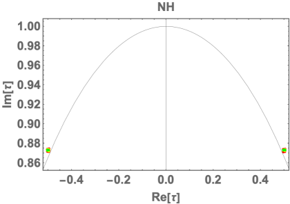
Figure 1: Allowed region for real $\tau$ and imaginary $\tau$ in NH.

In Fig. 1, we show the allowed region of $\tau$, and find that the allowed region is located at nearby $\tau=e^{2\pi i/3}$.

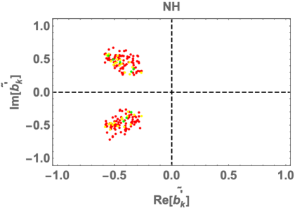
Figure 2: Allowed region for real $\tilde{b}^{\prime}_{k}$ and imaginary $\tilde{b}^{\prime}_{k}$ in NH.

In Fig. 2, we also show the allowed region of $\tilde{b}^{\prime}_{k}$, and find that the allowed region is about ${\rm Re}[\tilde{b}^{\prime}_{k}]=[-0.6,-0.2]$ and $|{\rm Im}[\tilde{b}^{\prime}_{k}]|=[0.2,0.6]$.

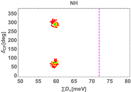
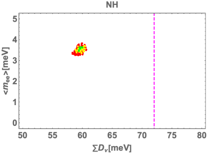
Figure 3: Allowed regions for $\delta_{CP}$ deg (left) and $\langle m_{ee}\rangle$ meV (right) in terms of $\sum D_{\nu}$ meV in NH. The vertical magenta dotted line is upper bound on results of Planck+DESI Adame et al. (2024) $\sum D_{\nu}\leq$72 meV.

In Fig. 3, we show the allowed region for $\delta_{CP}$ deg (left) and $\langle m_{ee}\rangle$ meV (right) in terms of $\sum D_{\nu}$ meV and find $\delta_{CP}=[30-100,270-330]$ deg, $\sum D_{\nu}=[58-61]$ meV, and $\langle m_{ee}\rangle=[3.2-4.0]$ meV. The vertical magenta dotted line is upper bound on results of Planck+DESI Adame et al. (2024) $\sum D_{\nu}\leq$72 meV.

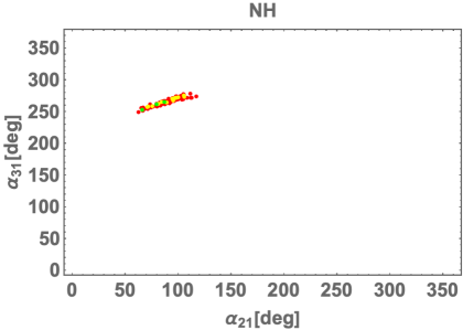
Figure 4: Allowed region for Majorana phases meV in NH.

In Fig. 4, we show the allowed region for Majorana phases and find $\alpha_{31}=[240-280]$ deg and $\alpha_{21}=[60-120]$ deg.

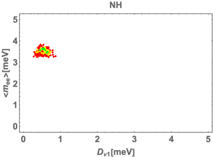
Figure 5: Allowed region for $\langle m_{ee}\rangle$ in terms of the lightest active neutrino mass in NH.

In addition, in Fig. 5, we show the allowed region for $\langle m_{ee}\rangle$ in terms of the lightest active neutrino mass in NH and find the lightest active neutrino mass to be $D_{\nu_{1}}=[0.2-1]$ meV.

III.2 IH

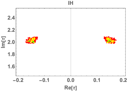
Figure 6: Allowed region for real $\tau$ and imaginary $\tau$ in IH.

In Fig. 6, we show the allowed region of $\tau$, and find that the allowed region is located at nearby $|{\rm Re}\tau|=[0.12-0.18]$ and ${\rm Im}\tau=[1.95-2.10]$.

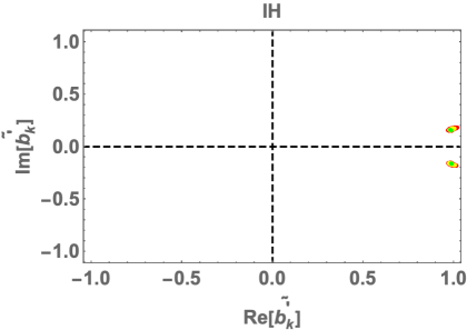
Figure 7: Allowed region for real $\tilde{b}^{\prime}_{k}$ and imaginary $\tilde{b}^{\prime}_{k}$ in IH.

In Fig. 7, we show the allowed region of $\tilde{b}^{\prime}_{k}$, and find that the allowed region is about ${\rm Re}[\tilde{b}^{\prime}_{k}]\approx 1$ and $|{\rm Im}[\tilde{b}^{\prime}_{k}]|=[0.1-0.2]$.

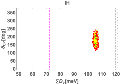
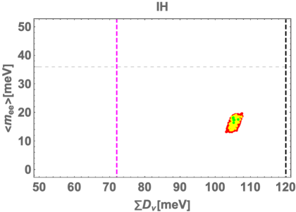
Figure 8: Allowed regions for $\delta_{CP}$ deg (left) and $\langle m_{ee}\rangle$ meV (right) in terms of $\sum D_{\nu}$ meV in IH. The vertical magenta and black dotted lines are respectively upper bound on results of Planck+DESI Adame et al. (2024); $\sum D_{\nu}\leq$72 meV and the minimal cosmological model $\Lambda$CDM $+\sum D_{\nu}$ Vagnozzi et al. (2017); Aghanim et al. (2020); $\sum D_{\nu}\leq$ 120 meV. The horizontal gray dotted line is lower bound on KamLAND-Zen data 36 meV.

In Fig. 8, we show the allowed region for $\delta_{CP}$ deg (left) and $\langle m_{ee}\rangle$ meV (right) in terms of $\sum D_{\nu}$ meV and find $\delta_{CP}=[120-250]$ deg, $\sum D_{\nu}=[102-108]$ meV, and $\langle m_{ee}\rangle=[12-20]$ meV. The vertical magenta and black dotted lines are respectively upper bound on results of Planck+DESI Adame et al. (2024); $\sum D_{\nu}\leq$72 meV and the minimal cosmological model $\Lambda$CDM $+\sum D_{\nu}$ Vagnozzi et al. (2017); Aghanim et al. (2020); $\sum D_{\nu}\leq$ 120 meV. The horizontal gray dotted line is the lower bound on the KamLAND-Zen data 36 meV.

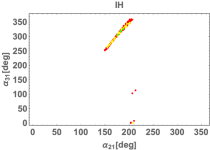
Figure 9: Allowed region for Majorana phases meV in IH.

In Fig. 9, we show the allowed region for Majorana phases and find $\alpha_{31}=[0-10,\ 100-120,\ 240-360]$ deg and $\alpha_{21}=[140-210]$ deg.

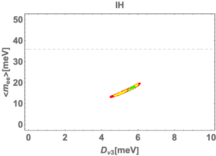
Figure 10: Allowed region for $\langle m_{ee}\rangle$ in terms of the lightest active neutrino mass in IH.

In Fig. 10, we show the allowed region for $\langle m_{ee}\rangle$ in terms of the lightest active neutrino mass in IH and find the lightest active neutrino mass to be $D_{\nu_{3}}=[4.5-6.2]$ meV.

IV Conclusions and discussions

We have investigated a Zee model applying a non-holomorphic modular $A_{4}$ symmetry, and we have obtained unique and sharp predictions for each of the normal and inverted hierarchy. This is because we have only two parameters in the neutrino sector including modulus $\tau$ due to appropriately assuming that the masses of charged-leptons are negligibly less than the masses for singly charged bosons.

Before closing this paper, we mention the constraints of Yukawa couplings $f$ and $y$. These main constraints come from lepton/hadron universalities which are induced at tree level and charged lepton flavor violations which are induced at one-loop level Herrero-Garcia et al. (2014); Okada (2015); Lindner et al. (2018). Even when we consider these bounds, it is totally safe if we take these Yukawa couplings are 0.01 in case of $m_{s}\sim m_{h^{\prime}}=$1 TeV. This value is easily achieved by adjusting the overall factor $a^{\prime}$ and $a_{s}$, which are parts of $\kappa$. Although $\kappa$ is fixed to fit the atmospheric mass squared difference, $\kappa$ can still maintain the fit value due to changing $\mu$ and $r$.

References

• Qu and Ding (2024) B.-Y. Qu and G.-J. Ding, JHEP 08, 136 (2024), eprint 2406.02527.
• Ding et al. (2024) G.-J. Ding, J.-N. Lu, S. T. Petcov, and B.-Y. Qu (2024), eprint 2408.15988.
• Li et al. (2024) C.-C. Li, J.-N. Lu, and G.-J. Ding (2024), eprint 2410.24103.
• Nomura and Okada (2024) T. Nomura and H. Okada (2024), eprint 2408.01143.
• Nomura et al. (2025) T. Nomura, H. Okada, and O. Popov, Phys. Lett. B 860, 139171 (2025), eprint 2409.12547.
• Zee (1980) A. Zee, Phys. Lett. B 93, 389 (1980), [Erratum: Phys.Lett.B 95, 461 (1980)].
• Ma (2006) E. Ma, Phys. Rev. D 73, 077301 (2006), eprint hep-ph/0601225.
• Nomura et al. (2021) T. Nomura, H. Okada, and Y.-h. Qi (2021), eprint 2111.10944.
• Abe et al. (2024) S. Abe et al. (KamLAND-Zen) (2024), eprint 2406.11438.
• Vagnozzi et al. (2017) S. Vagnozzi, E. Giusarma, O. Mena, K. Freese, M. Gerbino, S. Ho, and M. Lattanzi, Phys. Rev. D 96, 123503 (2017), eprint 1701.08172.
• Aghanim et al. (2020) N. Aghanim et al. (Planck), Astron. Astrophys. 641, A6 (2020), [Erratum: Astron.Astrophys. 652, C4 (2021)], eprint 1807.06209.
• Adame et al. (2024) A. G. Adame et al. (DESI) (2024), eprint 2404.03002.
• Esteban et al. (2024) I. Esteban, M. C. Gonzalez-Garcia, M. Maltoni, I. Martinez-Soler, J. a. P. Pinheiro, and T. Schwetz (2024), eprint 2410.05380.
• Herrero-Garcia et al. (2014) J. Herrero-Garcia, M. Nebot, N. Rius, and A. Santamaria, Nucl. Phys. B 885, 542 (2014), eprint 1402.4491.
• Okada (2015) H. Okada (2015), eprint 1503.04557.
• Lindner et al. (2018) M. Lindner, M. Platscher, and F. S. Queiroz, Phys. Rept. 731, 1 (2018), eprint 1610.06587.