Heterogeneous transfer learning for high dimensional regression with feature mismatch

Abstract

We consider the problem of transferring knowledge from a source, or proxy, domain to a new target domain for learning a high-dimensional regression model with possibly different features. Recently, the statistical properties of homogeneous transfer learning have been investigated. However, most homogeneous transfer and multi-task learning methods assume that the target and proxy domains have the same feature space, limiting their practical applicability. In applications, target and proxy feature spaces are frequently inherently different, for example, due to the inability to measure some variables in the target data-poor environments. Conversely, existing heterogeneous transfer learning methods do not provide statistical error guarantees, limiting their utility for scientific discovery. We propose a two-stage method that involves learning the relationship between the missing and observed features through a projection step in the proxy data and then solving a joint penalized regression optimization problem in the target data. We develop an upper bound on the method’s parameter estimation risk and prediction risk, assuming that the proxy and the target domain parameters are sparsely different. Our results elucidate how estimation and prediction error depend on the complexity of the model, sample size, the extent of overlap, and correlation between matched and mismatched features.

1 Introduction

The transfer learning problem considers a scenario with a target population on which we aim to infer a statistical model, perhaps a high-dimensional regression model. However, we have only limited data available from the target population. The model we wish to infer may have many more (even exponentially more) parameters in comparison to the sample size available in the target domain. On the other hand, we have a much larger dataset available from a proxy or source population whose characteristics are expected to be similar to the target population, but some parameters might differ between the populations. The general problem of transfer learning aims to transfer the knowledge learned in the proxy population to improve estimation and prediction on the target population.

In practical applications of transfer learning, several additional challenges appear, including differing sets of features or covariates between target and proxy data. For example, in a data-poor new environment, researchers may not only be limited by the sample size but also by the features on which they can collect data. Several methods have been proposed for transfer learning and multi-task learning in the last two decades (see Zhuang et al., (2020); Weiss et al., (2016) for comprehensive reviews). However, most transfer learning methods are developed for the homogeneous problem with target and source domains having the same feature space, which limits their practical applicability (Day and Khoshgoftaar,, 2017). As surveyed in Day and Khoshgoftaar, (2017), heterogeneous transfer learning (HTL) methods have been developed to bridge this gap. However, these HTL methods do not come with statistical guarantees for estimation and prediction error, limiting their utility for scientific discovery. In this article, we develop an HTL method for high-dimensional linear models to combine information from a proxy and a target population for improved estimation and prediction in the target population and study the statistical properties of the method.

Recently, several authors have studied the problem of transfer learning in various statistical problems, including high dimensional linear model (Bastani,, 2021; Li et al.,, 2022), generalized linear model (GLM)(Li et al., 2023c, ; Tian and Feng,, 2022), and graphical models (Li et al., 2023b, ). When the same set of covariates are available in both proxy and target data, and the difference between parameters in the two populations is a sparse vector, Bastani, (2021) and Takada and Fujisawa, (2020) proposed a joint estimation strategy based on $l_{1}$ penalized regression. The method proceeds by first computing the ordinary least squares (OLS) estimator of $\beta$ in proxy data, $\hat{\beta}_{\mathfrak{p}}$, and obtaining a modified response in the target population as $\tilde{\mathbf{y}}_{\mathfrak{t}}=\mathbf{y}_{\mathfrak{t}}-\mathbf{X}_{\mathfrak{t}}\hat{\beta}_{\mathfrak{p}}$. Then, the authors obtain the lasso estimator to learn the discrepancy parameter vector $\delta$ from the target data as $\hat{\delta}(\lambda)=\arg\min_{\delta}\|\tilde{\mathbf{y}}_{\mathfrak{t}}-\mathbf{X}_{\mathfrak{t}}\delta\|^{2}+\lambda\|\delta\|_{1}.$ Then, their final estimator becomes $\hat{\beta}_{\mathfrak{p}}+\hat{\delta}$. Bastani, (2021) provided a high probability upper bound on the estimation error for this estimator and showed that this upper bound is smaller than the lower bound of the OLS estimation on the target population alone, thereby establishing the superiority of their approach. A similar method was developed for the case when multiple source proxy datasets are available in Li et al., (2022), who also obtained minimax optimal rates of estimation error and showed that their “translasso” algorithm achieves the optimal error rate. Transfer learning approaches have been proposed in the context of high dimensional GLM with the discrepancy between source and target coefficients being $l_{1}$ sparse (Tian and Feng,, 2022). A similar methodology was obtained for GLM with a focus on developing inference in Li et al., 2023c . Transfer learning for Gaussian graphical models has been considered in Li et al., 2023b . A federated transfer learning approach for transferring knowledge across heterogeneous populations has been proposed in Li et al., 2023a . Transfer learning methods for nonparametric classification and regression problems with differential privacy constraints have been developed in Auddy et al., (2024) and Cai and Pu, (2024). A transfer learning method for high dimensional regression capable of handling shift in covariate distributions was developed recently in He et al., (2024).

Although several of the above approaches provide statistical theory, those approaches have a key limitation. They assume that the exact same set of covariates or features are available in both the target and proxy populations. However, this assumption is unrealistic in several applied settings. For example, in biomedical studies, the target domain could be a smaller dataset on a specific patient population measuring a few key covariates, while the proxy population could be obtained from the electronic health record where more information is available. The problem of learning with heterogeneous feature spaces in the proxy datasets has been explored in the literature Wiens et al., (2014); Yoon et al., (2018), but typically, these methods with different features do not come with statistical error guarantees. In this article, we develop a heterogeneous transfer learning method for learning a high-dimensional linear regression model in a target population using information from a related source dataset. We assume that some features are available only in the proxy domain and not in the target domain. We further assume that the missing features are related to the observed features, allowing us to estimate their values in the target data using a feature map learned from the proxy data. We rigorously study the estimation and prediction error from our methods and provide high probability upper bounds. We then extend this method to the case when multiple proxy datasets are available.

Our results suggest that the estimation error is related to target and proxy domain sample sizes, the complexity of the model, properties of the feature map relating the matched and mismatched features, and the discrepancy between the target and proxy domain parameters. The results indicate that the estimation error increases as the parameters between the two domains differ more, and the number of parameters of the model increases while it decreases with increasing sample size of the target domain. Further, the estimation error increases as the association between matched and mismatched features decreases. However, the results also indicate that it is possible to estimate models with an exponentially large number of parameters compared to the target sample size with successful transfer from a vast proxy dataset. We also show that the upper bound of the estimation error is smaller compared to what we would have if we chose to ignore the mismatched features and applied the method by Bastani, (2021) to the matched features only. In terms of prediction error, our results bring out the additional error made with respect to the result in Li et al., (2022) due to not observing a set of features directly and incurring loss due to imputation. As Day and Khoshgoftaar, (2017) notes in their survey of HTL methods that require “limited target labels”, that most of HTL methods in the literature do not provide how many samples would be considered “limited”. Our work answers that question by providing a bound that relates the target domain sample size with the discrepancy between target and source domains. Our simulation results confirm the theoretical results in finite samples. We see improved prediction error and estimation error with our HTL method compared to homogeneous TL and lasso on the target data.

Two papers related to ours are the recent works by Zhao et al., (2023) and Zhang et al., (2024), who considered the problems of heterogeneous transfer learning when there is a covariate mismatch between source and target domains and when only some of the covariate effects are transferable respectively. There are several differences between our framework and that of Zhao et al., (2023). While Zhao et al., (2023) focuses on the case when “summary-level” information from an external (proxy) study is available in addition to individual-level data from a main study (target data), our setup poses individual-level data availability in both domains allowing us to introduce and learn a feature map. Moreover, while Zhao et al., (2023) develop asymptotic results, our theoretical results focus on providing nonasymptotic upper bounds on estimation risk and prediction risk for learning models with possibly exponentially more parameters than target domain sample size. Importantly, unlike Zhao et al., (2023), we do not assume that the parameters corresponding to the common features are the same between proxy and target domains, but instead only assume that their difference is sparse. On the other hand, Zhang et al., (2024) considers the possibility that some features in a proxy dataset are relevant to the target domain problem and transferrable while other features are not. The authors then develop a Bayesian approach with covariate specific spike and slab prior to model partial similarities across domains. However, our framework is different from this work since we assume that some required covariates are unavailable in the target domain, while in the framework of Zhang et al., (2024), all covariates are available in all domains, but the effect of some covariates are different across domains making them non-transferable. In particular, Zhang et al., (2024) needs to assume that the change in the effect of the non-transferable covariates does not change the effect of the transferable covariates, which is difficult to guarantee in linear models since the parameters depend on what other covariates are in the model. In contrast, we provide an end-to-end solution that includes estimation in the proxy domain, which gives practitioners tools to transfer knowledge when some covariates are not available.

The rest of the paper is organized as follows. In Section 2, we describe our model and method for one source and one target population, in Section 3, we present theoretical results, in Section 4, we extend the methods and results to the case of multiple proxy or source datasets, in Section 5, we describe results from a simulation study, while Section 6 considers a case study on gene expression data.

2 Heterogeneous transfer learning with covariate mismatch

We first consider transferring knowledge from a single proxy dataset and will later generalize it to the case of multiple proxy datasets. Accordingly, suppose that we have a single proxy study that is informative for a predictive task on the target domain. Let $\mathbf{X}\in\mathbb{R}^{n\times p}$ and $\mathbf{y}=(Y_{1},\dots,Y_{n})^{\prime}\in\mathbb{R}^{n}$ denote design matrix and response vector, respectively. Rows of $\mathbf{X}$, denoted by $\mathbf{x}:=\left({\mathbf{x}_{1}}^{\prime},{\mathbf{x}_{2}}^{\prime}\right)^{\prime}$, contain matched features $\mathbf{x}_{1}\in\mathbb{R}^{p_{1}}$ that are assumed to be common in both proxy and target populations and mismatched features $\mathbf{x}_{2}\in\mathbb{R}^{p_{2}}$ that are not observed in the target domain. Accordingly, $\mathbf{X}_{1}\in\mathbb{R}^{n\times{p_{1}}}$ and $\mathbf{X}_{2}\in\mathbb{R}^{n\times{p_{2}}}$ denote the design matrices corresponding to matched and mismatched features, so the original design matrix can be partitioned as $\mathbf{X}=\left[\mathbf{X}_{1}|\mathbf{X}_{2}\right]$ and $p={p_{1}}+{p_{2}}$. From now on, let us use subscripts $\mathfrak{p}$ and $\mathfrak{t}$ to indicate the proxy and target domain, respectively. Then, consider the following data generating processes for a target data $\left\{{\mathbf{X}_{\mathfrak{t}}},\mathbf{y}_{\mathfrak{t}}\right\}$ and proxy data $\left\{\mathbf{X}_{\mathfrak{p}},\mathbf{y}_{\mathfrak{p}}\right\}$, respectively:

$$Y_{\mathfrak{t}}={\mathbf{x}_{1\mathfrak{t}}}^{\prime}\beta^{*}_{1\mathfrak{t}}+{\mathbf{x}_{2\mathfrak{t}}}^{\prime}\beta^{*}_{2\mathfrak{t}}+\epsilon_{\mathfrak{t}}\quad\quad Y_{\mathfrak{p}}={\mathbf{x}_{1\mathfrak{p}}}^{\prime}\beta^{*}_{1\mathfrak{p}}+{\mathbf{x}_{2\mathfrak{p}}}^{\prime}\beta^{*}_{2\mathfrak{p}}+\epsilon_{\mathfrak{p}}$$

for zero-mean errors $\epsilon_{\mathfrak{t}}$ and $\epsilon_{\mathfrak{p}}$. We observe ${n_{\mathfrak{t}}}$ sample points from the target domain and $n_{\mathfrak{p}}$ from the proxy domain. The objective of transfer learning is to leverage information from proxy data in order to enhance our estimator for the parameter in the data generating process of the target data (i.e., $\beta^{*}_{1\mathfrak{t}},\beta^{*}_{2\mathfrak{t}}$), which in turn could lead to lower prediction error in the target domain. However, certain covariates may be unavailable in the target domain, even though we have complete data available in the proxy population. Specifically, in model (2), we consider the scenario where only the covariates $\mathbf{X}_{1}$ are accessible in the target population, while the covariates $\mathbf{X}_{2}$ are not. We are, however, able to observe both $\mathbf{X}_{1}$ and $\mathbf{X}_{2}$ in the proxy population.

We posit that the differences in covariate effects are sparse in the sense that $\delta_{l}^{*}=\beta^{*}_{l\mathfrak{t}}-\beta^{*}_{l\mathfrak{p}}$, is a sparse vector for $l=1,2$, either in the $\ell_{0}$ or $\ell_{1}$ sense. The primary objective of our inference is to estimate $(\beta^{*}_{1\mathfrak{t}},\beta^{*}_{2\mathfrak{t}})$. We emphasize that the true data-generating process in the target population requires both $\mathbf{X}_{1}$ and $\mathbf{X}_{2}$, but only $\mathbf{X}_{1}$ is available to us in the training samples and any future prediction tasks. Therefore, when we compare prediction errors of the methods, we assume the test data is generated following the data generation process of the target data, yet only $\mathbf{X}_{2}$ will be available in the test data. We also note that we do not assume the regression model parameters, even for the matched features, to be the same across the domains.

2.1 Random designs and notations

Define a $p$-dimensional unit sphere as $S^{p-1}=\left\{\mathbf{x}\in\mathbb{R}^{p};\|\mathbf{x}\|=1\right\}$. Given a real-valued random variable $\mathbf{X}$, denote its sub-gaussian norm by $\|X\|_{\psi_{2}}:=\inf\left\{t>0;\mathbb{E}\exp\left(X^{2}/t^{2}\right)\leq 2\right\}$. For a matrix $\mathbf{X}_{n\times p}$, we denote its $i$-th row and $j$-th column by $\mathbf{X}_{i\cdot}\in\mathbb{R}^{p}$ and $\mathbf{X}_{\cdot j}\in\mathbb{R}^{n}$, respectively. We write $\lambda_{\min}(\mathbf{A})$ and $s_{\min}(\mathbf{A})$ to denote the minimum eigenvalue and the minimum singular value ($\lambda_{\max},s_{\max}$ are used analogously) of $\mathbf{A}$. Also, write $\mathbf{A}\succcurlyeq\mathbf{B}$ if $\mathbf{A}-\mathbf{B}$ is positive semi-definite, i.e., $\mathbf{x}^{\prime}\left(\mathbf{A}-\mathbf{B}\right)\mathbf{x}\geq 0$ for any $\mathbf{x}\in S^{p-1}$. Write $\|\mathbf{x}\|_{\mathbf{D}}^{2}:=\mathbf{x}^{\prime}\mathbf{D}\mathbf{x}$ which is non-negative if $\mathbf{D}$ is positive semi-definite. For an index set $A=[p]$ of a vector $\mathbf{x}\in\mathbb{R}^{p}$, define $\mathbf{x}_{A}$ as $(\mathbf{x}_{A})_{i}:=x_{i}1(i\in A)$ for $i=1,...,p$. For the convenience of asymptotics, we denote generic positive constants by $c,\tilde{c},c^{\prime}$, and so on. We write $a_{n}=O(b_{n})$ if $\lim\sup_{n\to\infty}\frac{a_{n}}{b_{n}}<\infty$, $a_{n}=o(b_{n})$ if $\lim_{n\to\infty}\frac{a_{n}}{b_{n}}=0$, and $a_{n}\asymp b_{n}$ if $a_{n}=O(b_{n})$ and $b_{n}=O(a_{n})$. Also, write $a_{n}=\Omega(b_{n})$ if $\lim\sup_{n\to\infty}\frac{a_{n}}{b_{n}}>0$ and $a_{n}=\omega\left(b_{n}\right)$ if $\lim_{n\to\infty}\frac{a_{n}}{b_{n}}=\infty$. Let $\|\mathbf{A}\|_{p}:=\sup_{\mathbf{u}\in\mathcal{S}^{d-1}}\|\mathbf{A}\mathbf{u}\|_{p}$ denote the matrix $\ell_{p}$ norm induced by vector $\ell_{p}$ norms for any $\mathbf{A}\in\mathbb{R}^{n\times d}$ and $p>0$. For the case of $p=2$, which is the same as the spectral norm, we use the notation $\|\mathbf{A}\|$ for simplicity.

Our methodology involves estimating the missing covariates $\mathbf{X}_{2}$ in the target data with the help of a feature map learned from the proxy data. This imputation methodology is based on the covariance structure of the random feature vectors. To proceed, we need a few definitions. The following gives the formal definitions of sub-gaussian random variables, random vectors, and random ensembles used in this paper.

Definition 1.

A zero-mean random variable $X$ is said to be a $\sigma$-sub-gaussian random variable if there exists a constant $\sigma>0$ such that $\mathbb{E}\exp\left(uX\right)\leq\exp(u^{2}\sigma^{2}/2)$ for any $u\in\mathbb{R}$. Then, we write $X\sim SG(\sigma)$.

Definition 2.

If a zero-mean random vector $\mathbf{x}\in\mathbb{R}^{d}$ satisfies $\mathbf{u}^{\prime}\mathbf{x}\sim SG(\sigma)$ for all $\mathbf{u}\in S^{d-1}$, then we say $\mathbf{x}$ is a $\sigma$-sub-gaussian random vector and write $\mathbf{x}\sim SG(\sigma)$.

Definition 3.

If the rows of a centered random matrix $\mathbf{X}\in\mathbb{R}^{n\times d}$, $\mathbf{x}_{1},...,\mathbf{x}_{n}$, are i.i.d. $\sigma$-sub-gaussian random vectors, then we say $\mathbf{X}$ is a row-wise $\sigma$-sub-gaussian ensemble and write $\mathbf{X}\sim SG(\sigma)$.

Sub-gaussian distributions can include a variety of distributions (discrete or continuous, bounded and sub-gaussian-tailed), so they are a reasonable choice for a random design regression model. We assume that the zero-mean covariates $\mathbf{x}_{1}\in\mathbb{R}^{{p_{1}}}$ which is common for both domains is a $\sigma_{1}$-sub-gaussian random vector for $\sigma_{1}>0$. i.e., $\mathbf{x}_{1}\sim SG(\sigma_{1})$. Accordingly, we assume that $\mathbf{X}_{1}$ is row-wise $\sigma_{1}$-sub-gaussian ensemble with $n$ independent rows and $p$ columns. Then, we specify the following linear process for $\mathbf{X}_{2}$ for both the target and proxy data:

$$\mathbf{X}_{2}=\mathbf{X}_{1}\Theta+\Xi,\ \text{where}\ \mathbf{X}_{1}\sim SG(\sigma_{1})\ \bot\ \Xi_{n\times{p_{2}}}\sim SG(\sigma_{\xi}).$$ (1)

Note the matrices $\mathbf{X}_{1}$ and $\Xi$ are sub-gaussian ensembles independent of each other. This assumption is equivalent to assuming that a linear map of matched covariates can recover the mismatched covariates approximately. For the proxy domain, this corresponds to an equation $\mathbf{X}_{2\mathfrak{p}}=\mathbf{X}_{1\mathfrak{p}}\Theta_{\mathfrak{p}}+\Xi_{\mathfrak{p}}$, and ${\mathbf{X}_{2\mathfrak{t}}}={\mathbf{X}_{1\mathfrak{t}}}\Theta_{\mathfrak{t}}+\Xi_{\mathfrak{t}}$ for the target population. Write the maximum singular value of $\Theta_{\mathfrak{p}}\in\mathbb{R}^{{p_{1}}\times{p_{2}}}$ as $\theta_{\mathfrak{p}}:=\left\|\Theta_{\mathfrak{p}}\right\|$, and define $\theta_{\mathfrak{t}}$ similarly. As a consequence, since $\mathbf{X}_{1}$ and $\Xi$ are assumed to be independent, we notice that $\mathbf{X}_{2}\sim SG(\sigma_{2})$ where $\sigma_{2}:=\sigma_{1}\theta+\sigma_{\xi}$ by the convenient results that we prove in Lemmas E.3 and E.4 in Appendix E. Therefore $\mathbf{X}_{2}$ is also a sub-gaussian ensemble. We have the random design matrix as $\mathbf{X}=\left[\mathbf{X}_{1}|\mathbf{X}_{2}\right]\in\mathbb{R}^{n\times p}$, and hence $\mathbf{X}\sim SG\left(\sigma_{1}+\sigma_{2}\right)$. Then, we can denote ${\sigma_{\mathfrak{p}}}:={\sigma_{1\mathfrak{p}}}+\sigma_{2\mathfrak{p}}={\sigma_{1\mathfrak{p}}}(1+\theta_{\mathfrak{p}})+{\sigma_{\xi\mathfrak{p}}}$ and ${\sigma_{\mathfrak{t}}}:={\sigma_{1\mathfrak{t}}}+\sigma_{2\mathfrak{t}}={\sigma_{1\mathfrak{t}}}(1+\theta_{\mathfrak{t}})+{\sigma_{\xi\mathfrak{t}}}$.

For both the target and proxy populations, we have the covariance matrix $\Sigma$ of $\mathbf{X}$ as

$$\begin{bmatrix}\Sigma_{11}&\Sigma_{12}\\ \Sigma_{21}&\Sigma_{22}\end{bmatrix}:=\begin{bmatrix}\Sigma_{11}&\Sigma_{11}\Theta\\ \Theta^{\prime}\Sigma_{11}&\Theta^{\prime}\Sigma_{11}\Theta+\Sigma_{\xi}\end{bmatrix}$$

by construction of $\mathbf{X}_{1}$ and $\mathbf{X}_{2}$. Denote the minimum and maximum eigenvalue of $\Sigma$ as $\rho:=\lambda_{\min}(\Sigma)$ and $\tau:=\lambda_{\max}(\Sigma)$, respectively. Accordingly, $\rho_{1},\tau_{1}$ and $\rho_{2},\tau_{2}$ will represent those of $\Sigma_{11}$ and $\Sigma_{22}$. Then, from our model setup, by the property of sub-gaussians (see Appendix E) we have $\tau_{1}\leq{\sigma_{1}}^{2}$ and $\tau\leq\sigma^{2}$.

2.2 Assumptions

We make a few assumptions on the feature map, covariates in the proxy population and regression coefficients.

Assumption 1 (Feature map).

Assume that $\theta_{\mathfrak{t}}$ and $\theta_{\mathfrak{p}}$ are bounded above by some positive constant. Further, assume that $\left\|\Theta_{\mathfrak{t}}-\Theta_{\mathfrak{p}}\right\|\leq\delta_{\theta}$ for some constant $\delta_{\theta}>0$.

Assumption 2 (Proxy Population).

The matched covariates in the proxy domain satisfy $n_{\mathfrak{p}}\geq{p_{1}}$ and ${\mathbf{X}_{1\mathfrak{p}}}^{\prime}\mathbf{X}_{1\mathfrak{p}}=n_{\mathfrak{p}}\mathbf{I}_{p_{1}}$, i.e., columns of $\mathbf{X}_{1\mathfrak{p}}$ are standardized and orthogonal. Further, we assume that the eigenvalues of $\Sigma_{1\mathfrak{p}}$ are all bounded below from zero and above by infinity for all $k$.

Assumption 3 (Bounded regression coefficients).

There exists some positive constant $b_{\beta}>0$ that bounds the true target regression coefficient as $\|\beta_{\mathfrak{t}}^{*}\|_{1}\leq b_{\beta}$.

The first assumption allows for the possibility that the feature maps that describe the relationship between $\mathbf{X}_{1}$ and $\mathbf{X}_{2}$ may differ between the target and proxy populations, but the difference between them in spectral norm is bounded. In simulations, we observe that if the difference between the feature maps in proxy and target data are too large, then the performance of our procedure deteriorates. This is expected since in the absence of $\mathbf{X}_{2}$ in the target data, we have no way to calibrate the feature map between $\mathbf{X}_{1}$ and $\mathbf{X}_{2}$ in target data. Hence, we need $\mathbf{X}_{2}$ and $\mathbf{X}_{1}$ to be related and the relationship between them to remain somewhat consistent across populations. The second assumption says that the sample size in the proxy domain is larger than the number of covariates in $\mathbf{X}_{1}$. Note we make no such assumption on the sample size of the target domain and we will assume the sample size in target domain is much less. The third assumption is a standard assumption that says the coefficient vector in the target domain is bounded by some constant.

Now, let us write the cardinality of a set $A$ as $|A|$. The following definition is introduced as a compatibility condition in studying our random design regression model.

Definition 4.

We say that an index set $A\subseteq\left[p\right]$ and a positive semi-definite matrix $\mathbf{L}\in\mathbb{R}^{p\times p}$ meet the compatibility condition if there exist a diagonal matrix $\mathbf{D}$ with positive diagonal entries and $\phi>0$ such that

$$\|\mathbf{u}_{A}\|_{1}^{2}\leq\frac{|A|}{\phi^{2}}\|\mathbf{u}\|_{\mathbf{D}\mathbf{L}\mathbf{D}}^{2}~~\forall\,\mathbf{u}\in\mathbb{R}^{p}\text{ such that }\|\mathbf{u}_{A^{c}}\|_{1}\leq 3\|\mathbf{u}_{A}\|_{1}.$$

Compatibility condition requires the $\ell_{1}$-norm and the $\ell_{2}$-norm to be compatible (van de Geer and Bühlmann,, 2009). Note that our definition above slightly differs from the definition prevalent in literature as we require more than one tuning parameters in studying the objective function. If we take $\mathbf{D}=\mathbf{I}_{p}$ and consider $\mathbf{L}=\frac{1}{n}\mathbf{X}^{\prime}\mathbf{X}$ for a fixed design case, the above definition reduces to the compatibility condition for fixed design regression. Let $S:=S_{1}\cup S_{2}$ where $S_{1}:=\operatorname{supp}(\delta_{1}^{*})\subseteq[{p_{1}}]$ and $S_{2}:=\operatorname{supp}(\mathbf{o}_{p_{1}},\delta_{2}^{*})\subseteq\left\{{p_{1}}+1,...,p\right\}$. Therefore, the set $S$ denotes the support of the discrepancy between the parameters in the target and source domains. The cardinality of this set $|S|$ plays an important role in our theoretical results. By Theorem D.2 in Appendix D, taking the set $A=S$ in Definition 4 and the sample covariance with our imputed design matrix as $\mathbf{L}$, meet compatibility condition with high probability. We utilize this to obtain non-asymptotic upper bounds for estimation and prediction errors.

2.3 Heterogeneous transfer learning

Now, we propose the following two-stage estimator for transfer learning with feature mismatch that includes an imputation step and an estimation step.

1. Imputation

   1. $\hat{\Theta}_{\mathfrak{p}}=({\mathbf{X}_{1\mathfrak{p}}}^{\prime}\mathbf{X}_{1\mathfrak{p}})^{-1}{\mathbf{X}_{1\mathfrak{p}}}^{\prime}\mathbf{X}_{2\mathfrak{p}}$,  $\hat{\mathbf{X}}_{2\mathfrak{t}}:={\mathbf{X}_{1\mathfrak{t}}}\hat{\Theta}_{\mathfrak{p}}$

2. Estimation

   1. $\hat{\beta}_{\mathfrak{p}}^{ht}=\arg\min_{\beta_{1},\beta_{2}}\left\{\frac{1}{n_{\mathfrak{p}}}\left\|\mathbf{y}_{\mathfrak{p}}-\mathbf{X}_{1\mathfrak{p}}\beta_{1}-\mathbf{X}_{2\mathfrak{p}}\beta_{2}\right\|^{2}\right\}$

   2. $\hat{\beta}_{\mathfrak{t}}^{ht}=\arg\min_{\beta_{1},\beta_{2}}\left\{\frac{1}{{n_{\mathfrak{t}}}}\|\mathbf{y}_{\mathfrak{t}}-{\mathbf{X}_{1\mathfrak{t}}}\beta_{1}-\hat{\mathbf{X}}_{2\mathfrak{t}}{\beta}_{2}\|^{2}+\sum_{l=1}^{2}\lambda_{l}\|\beta_{l}-\hat{\beta}_{l\mathfrak{p}}^{ht}\|_{1}\right\}$

In the first stage, which we call the imputation stage, we obtain a projection (feature map) of the covariates in $\mathbf{X}_{2}$ onto the covariates in $\mathbf{X}_{1}$ using the proxy data. Then in the target data, we approximate $\hat{\mathbf{X}}_{2\mathfrak{t}}$ using ${\mathbf{X}_{1\mathfrak{t}}}$ and this projection learned from the proxy population. Under Assumption 2 and using relationship Equation 1, we have

$$\hat{\Theta}_{\mathfrak{p}}=\frac{1}{n_{\mathfrak{p}}}{\mathbf{X}_{1\mathfrak{p}}}^{\prime}\mathbf{X}_{2\mathfrak{p}}=\Theta_{\mathfrak{p}}+\frac{1}{n_{\mathfrak{p}}}{\mathbf{X}_{1\mathfrak{p}}}^{\prime}\Xi_{\mathfrak{p}}.$$

We assume in Assumption 2 that the proxy domain has enough data such that $({\mathbf{X}_{1\mathfrak{p}}}^{\prime}\mathbf{X}_{1\mathfrak{p}})$ is invertible. Note that we do not require this to hold in the target data since it is expected that target data will have a much lower sample size than the number of covariates in $\mathbf{X}_{1\mathfrak{p}}$. If the proxy domain does not have enough sample size, then we propose to estimate the feature map using multivariate lasso or ridge regression.

We note that homogeneous transfer learning, where one leverages the knowledge of matched features only (e.g. Bastani,, 2021; Li et al.,, 2022), becomes a special case of our approach. This can be illustrated as ignoring the correlation between matched and mismatched features in the modeling process, thus transferring knowledge for estimating $\beta_{1\mathfrak{t}}$ only. As we assume that the effect size across target and proxy predictors are equal up to a shift by some sparse vector, we can leverage it to obtain a better approximate for $\beta_{1\mathfrak{t}}^{*}$. However, under our true data-generating model that includes both $\mathbf{X}_{1}$ and $\mathbf{X}_{2}$, this method will fit a misspecified model and therefore likely to incur large estimation and prediction errors. Therefore we will use this method as a baseline approach to compare our HTL method against. In particular, the joint estimation method proposed by Bastani, (2021), can be described as follows using our notation.

$$\hat{\beta}_{1\mathfrak{p}}^{hm} =\arg\min_{\beta_{1}}\frac{1}{n_{\mathfrak{p}}}\left\|\mathbf{y}_{\mathfrak{p}}-\mathbf{X}_{1\mathfrak{p}}\beta_{1}\right\|^{2},$$

$$\hat{\beta}_{1\mathfrak{t}}^{hm} =\arg\min_{\beta_{1}}\left\{\frac{1}{{n_{\mathfrak{t}}}}\|\mathbf{y}_{\mathfrak{t}}-{\mathbf{X}_{1\mathfrak{t}}}\beta_{1}\|^{2}+\lambda_{1}\|\beta_{1}-\hat{\beta}_{1\mathfrak{p}}^{hm}\|_{1}\right\}.$$

This strategy has proved to be superior in terms of estimation risk (Bastani,, 2021) compared to the ridge regression on target population or model averaging estimation strategy. We emphasize that since $\mathbf{X}_{2}$ is not available in the target domain a homogeneous transfer involving both $\mathbf{X}_{1}$ and $\mathbf{X}_{2}$ is not possible.

3 Theoretical properties of the HTL estimator

3.1 Estimation risk

Now, we obtain a high probability upper bound on the estimation error and evaluate the estimation risk of proposed heterogeneous transfer learning for estimating the parameters of the target domain model. Following Bastani, (2021), we use the parameter estimation risk with $\ell_{1}$ loss function as the metric of evaluation, $\mathcal{R}(\hat{\beta},\beta^{*}_{\mathfrak{t}})=\mathbb{E}\left\|\hat{\beta}-\beta^{*}_{\mathfrak{t}}\right\|_{1}$. For the proof of the results presented in this section, we refer the readers to Section B of the Appendix as HTL with single proxy study corresponds to the HTL with $K$ proxy studies when $K=1$.

Let us write $\mathbf{\cal E}_{\mathfrak{t}}=\left(\epsilon_{1,\mathfrak{t}},...,\epsilon_{{n_{\mathfrak{t}}},\mathfrak{t}}\right)^{\prime}$ to denote the target model errors. Let $\tilde{\delta}_{l}^{ht}:=\beta_{l\mathfrak{t}}^{*}-\hat{\beta}_{l\mathfrak{p}}^{ht}$, and $\delta_{l}^{ht}:=\beta_{l}-\hat{\beta}_{l\mathfrak{p}}^{ht}$, denote discrepancy vector of estimated proxy domain parameter vector $\hat{\beta}_{l\mathfrak{p}}^{ht}$ from the true parameter vector $\beta_{l\mathfrak{t}}^{*}$ and an arbitrary parameter vector $\beta_{l}$ respectively. Also, let $\nu_{l}^{ht}:=\hat{\beta}_{l\mathfrak{p}}^{ht}-\beta_{l\mathfrak{p}}$ denote the approximation errors for the proxy domain parameters for $l=1,2$. With the imputation of ${\mathbf{X}_{2\mathfrak{t}}}$, finding $\hat{\beta}_{\mathfrak{t}}^{ht}$ is equivalent to finding $\delta^{ht}$ such that

$$\hat{\delta}^{ht} =\underset{\delta^{ht}\in\mathbb{R}^{p}}{\arg\min}\left\{\frac{1}{{n_{\mathfrak{t}}}}\left\|\mathbf{\cal E}_{\mathfrak{t}}+\sum_{l=1}^{2}\mathbf{X}_{l\mathfrak{t}}(\tilde{\delta}_{l}^{ht}-\delta_{l}^{ht})+\Delta\left(\beta_{2t}^{*}+\delta_{2}^{ht}-\tilde{\delta}_{2}^{ht}\right)\right\|^{2}+\sum_{l=1}^{2}\lambda_{l}\|\delta_{l}^{ht}\|_{1}\right\}$$ (2)

where $\Delta={\mathbf{X}_{2\mathfrak{t}}}-\hat{\mathbf{X}}_{2\mathfrak{t}}$ represents the imputation error of $\hat{\mathbf{X}}_{2\mathfrak{t}}$. Then, the proposed estimator takes the form of $\hat{\beta}_{\mathfrak{t}}^{ht}(\lambda_{1},\lambda_{2})=\hat{\beta}_{\mathfrak{p}}^{ht}+\hat{\delta}^{ht}(\lambda_{1},\lambda_{2})$. Next, let ${\tilde{\mathbf{X}}_{\mathfrak{t}}}:=\left[{\mathbf{X}_{1\mathfrak{t}}}|\hat{\mathbf{X}}_{2\mathfrak{t}}\right]$ be an imputed target design matrix. Since our objective function is convex, for $\delta^{ht}=\hat{\delta}^{ht}$ and $\delta^{ht}=\tilde{\delta}^{ht}$ we have the following:

$$\frac{1}{{n_{\mathfrak{t}}}}\left\|\mathbf{\cal E}_{\mathfrak{t}}+\Delta\beta_{2t}^{*}+\sum_{l=1}^{2}\mathbf{X}_{l\mathfrak{t}}(\tilde{\delta}^{ht}_{l}-\hat{\delta}^{ht}_{l})+\Delta\left(\hat{\delta}^{ht}_{2}-\tilde{\delta}^{ht}_{2}\right)\right\|^{2}+\sum_{l=1}^{2}\lambda_{l}\|\hat{\delta}^{ht}_{l}\|_{1}$$

$$\leq\frac{1}{{n_{\mathfrak{t}}}}\|\mathbf{\cal E}_{\mathfrak{t}}+\Delta\beta_{2t}^{*}\|^{2}+\sum_{l=1}^{2}\lambda_{l}\|\tilde{\delta}^{ht}_{l}\|_{1}.$$

Write $\tilde{\delta}^{ht}-\hat{\delta}^{ht}=\begin{bmatrix}\tilde{\delta}^{ht}_{1}-\hat{\delta}^{ht}_{1}\\ \tilde{\delta}^{ht}_{2}-\hat{\delta}^{ht}_{2}\end{bmatrix}$. Then, $\sum_{l}\mathbf{X}_{l\mathfrak{t}}(\tilde{\delta}^{ht}_{l}-\hat{\delta}^{ht}_{l})+\Delta\left(\hat{\delta}^{ht}_{2}-\tilde{\delta}^{ht}_{2}\right)={\tilde{\mathbf{X}}_{\mathfrak{t}}}(\tilde{\delta}^{ht}-\hat{\delta}^{ht})$, and

$$\frac{1}{{n_{\mathfrak{t}}}}\|{\tilde{\mathbf{X}}_{\mathfrak{t}}}(\tilde{\delta}^{ht}-\hat{\delta}^{ht})\|^{2}+\sum_{l=1}^{2}\lambda_{l}\|\hat{\delta}^{ht}_{l}\|_{1}\leq\frac{2}{{n_{\mathfrak{t}}}}\left(\mathbf{\cal E}_{\mathfrak{t}}+\Delta\beta_{2t}^{*}\right)^{\prime}{\tilde{\mathbf{X}}_{\mathfrak{t}}}(\hat{\delta}^{ht}-\tilde{\delta}^{ht})+\sum_{l=1}^{2}\lambda_{l}\|\tilde{\delta}^{ht}_{l}\|_{1}.$$

Therefore, we have the inequality

$$\frac{1}{{n_{\mathfrak{t}}}}\|{\tilde{\mathbf{X}}_{\mathfrak{t}}}(\tilde{\delta}^{ht}-\hat{\delta}^{ht})\|^{2}+\sum_{l=1}^{2}\lambda_{l}\|\hat{\delta}^{ht}_{l}\|_{1}\leq\frac{2}{{n_{\mathfrak{t}}}}\|\left(\mathbf{\cal E}_{\mathfrak{t}}+\Delta\beta_{2t}^{*}\right)^{\prime}{\tilde{\mathbf{X}}_{\mathfrak{t}}}\|_{\infty}\|\hat{\delta}^{ht}-\tilde{\delta}^{ht}\|_{1}+\sum_{l=1}^{2}\lambda_{l}\|\tilde{\delta}^{ht}_{l}\|_{1}.$$

Compared to the case of homogeneous transfer learning, since we imputed the missing signal ${\mathbf{X}_{2\mathfrak{t}}}\beta^{*}_{2}$, an additional error term $\Delta$ and $\hat{\mathbf{X}}_{2t}$ need to be controlled in the theoretical analyses.

The following lemma is an intermediate result that provides a high-probability upper bound on the estimation error of $\beta_{t}^{*}$ using the HTL estimator with user-chosen tuning parameter $\lambda$, that brings out dependencies of the estimation error on several model parameters.

Lemma 3.1.

Let $r:=\frac{{p_{1}}{\sigma_{\xi\mathfrak{p}}}^{2}{\sigma_{1\mathfrak{t}}}^{2}}{n_{\mathfrak{p}}}$, $\phi$ be the compatibility constant, and

$$\zeta:=\left[\sigma_{\epsilon\mathfrak{t}}+\left\{{\sigma_{\xi\mathfrak{t}}}+{\sigma_{1\mathfrak{t}}}\left(\delta_{\theta}+\frac{\sqrt{6{p_{1}}}{\sigma_{\xi\mathfrak{p}}}}{\sqrt[4]{n_{\mathfrak{p}}}}\right)\right\}b_{\beta}\right]{\sigma_{1\mathfrak{t}}}\left(1+\theta_{\mathfrak{p}}+\frac{\sqrt{6{p_{1}}}{\sigma_{\xi\mathfrak{p}}}}{\sqrt[4]{n_{\mathfrak{p}}}}\right),$$

and let positive quantities $\lambda$, $n_{\mathfrak{p}}$ satisfy $10rb_{\beta}<\lambda<\frac{p{\sigma_{\mathfrak{p}}}\sigma_{\epsilon\mathfrak{p}}}{\rho_{\mathfrak{p}}}$. Then, we have

$$\|\hat{\beta}_{\mathfrak{t}}^{ht}-\beta_{\mathfrak{t}}^{*}\|_{1}\leq 5\lambda\left\{\frac{{\sigma_{1\mathfrak{t}}}^{2}}{p}\left(1+\theta_{\mathfrak{p}}^{2}+\frac{{p_{1}}{\sigma_{\xi\mathfrak{p}}}^{2}}{n_{\mathfrak{p}}}\right)+1+\frac{|S|}{\phi^{2}}\right\}$$

with probability at least $1-C^{\prime}\pi_{\delta^{ht}}\left(\lambda\right)$ where

$$\pi_{\delta^{ht}}\left(\lambda\right):= \ p\left[e^{{p_{2}}\log 7-c\sqrt{n_{\mathfrak{p}}}{p_{1}}}+e^{-c{n_{\mathfrak{t}}}\min\left(g(\lambda),g(\lambda)^{2}\right)}+\exp\left(-\frac{cn_{\mathfrak{p}}\lambda^{2}{\rho_{\mathfrak{p}}}^{2}}{p^{2}{\sigma_{\mathfrak{p}}}^{2}\sigma_{\epsilon\mathfrak{p}}^{2}}\right)\right]$$

$$+\exp\left\{-\frac{c{n_{\mathfrak{t}}}\tau_{1\mathfrak{t}}^{2}\left(1+{\theta_{\mathfrak{p}}}^{2}\right)^{2}}{{\sigma_{1\mathfrak{t}}}^{4}\left(1+{\theta_{\mathfrak{p}}}^{2}+\frac{6{p_{1}}{\sigma_{\xi\mathfrak{p}}}^{2}}{\sqrt{n_{\mathfrak{p}}}}\right)^{2}}\right\}+\exp\left\{-\frac{c{n_{\mathfrak{t}}}{\rho_{1\mathfrak{t}}}^{2}}{{\sigma_{1\mathfrak{t}}}^{4}\left(1+{\theta_{\mathfrak{p}}}^{2}+\frac{6{p_{1}}{\sigma_{\xi\mathfrak{p}}}^{2}}{\sqrt{n_{\mathfrak{p}}}}\right)^{2}}\right\}$$

$$+\exp\left\{-\frac{cn_{\mathfrak{p}}}{{\sigma_{\mathfrak{p}}}^{4}}\left(\frac{1}{2}-c^{\prime}{\sigma_{\mathfrak{p}}}^{2}\sqrt{\frac{p}{n_{\mathfrak{p}}}}\right)^{2}\right\}.$$

for $g(\lambda):=\frac{1}{\zeta}\left(\frac{\lambda}{5}-2rb_{\beta}\right)$.

The next theorem is our main result, which, under some assumptions, provides a high-probability bound on the estimation loss of the HTL estimator and provides an upper bound on the estimation risk of a truncated version of the estimator.

Theorem 3.1.

Define a truncated estimator $\hat{\beta}_{\mathfrak{t},tr}^{ht}(\lambda):=\hat{\beta}_{\mathfrak{t}}^{ht}1_{\left\{\|\hat{\beta}_{\mathfrak{t}}^{ht}\|_{1}\leq 2b_{\beta}\right\}}$. Then, for $a\in(0,1)$ pick $\lambda=\max\left(\sqrt{\frac{p^{2}(\log p)^{1+a}}{n_{\mathfrak{p}}}},\frac{\log p}{{n_{\mathfrak{t}}}}\right)$ and assume that $n_{\mathfrak{p}}\asymp p^{2}(\log p)^{2}$ and the population variance proxies $\sigma_{\epsilon\mathfrak{t}},{\sigma_{\xi\mathfrak{t}}}$, and ${\sigma_{\xi\mathfrak{p}}}$ are $\mathcal{O}(1)$. Then, we have

1. $\|\hat{\beta}_{\mathfrak{t}}^{ht}-\beta_{\mathfrak{t}}^{*}\|_{1}=\mathcal{O}\left[|S|\left\{\left(\frac{1}{\log p}\right)^{\frac{1-a}{2}}+\frac{\log p}{{n_{\mathfrak{t}}}}\right\}\right]$ with probability at least

   $$1-\exp\left\{-c^{\prime}{n_{\mathfrak{t}}}{\rho_{1\mathfrak{t}}}^{2}\frac{p^{2}(\log p)^{2}}{{p_{1}}^{2}}\right\}-o(1).$$

2. $\mathcal{R}\left(\hat{\beta}_{\mathfrak{t},tr}^{ht},\beta^{*}_{\mathfrak{t}}\right)=\mathcal{O}\left[|S|\left\{\left(\frac{1}{\log p}\right)^{\frac{1-a}{2}}+\frac{\log p}{{n_{\mathfrak{t}}}}\right\}+\exp\left(-c^{\prime}{n_{\mathfrak{t}}}{\rho_{1\mathfrak{t}}}^{2}\frac{p^{2}(\log p)^{2}}{{p_{1}}^{2}}\right)\right].$

In the above theorem, we pick a $\lambda$ that makes most of the terms of $\pi_{\delta^{ht}}(\lambda)$ in Lemma 3.1 go to 0. In the first part, clearly, $\frac{n_{\mathfrak{t}}p^{2}(\log p)^{2}}{p_{1}^{2}}\to\infty$, since $p>p_{1}$ and both $p,n_{\mathfrak{t}}\to\infty$, and hence the upper bound on the estimation error holds with probability converging to 1. For the bound on the risk, as also noted in Bastani, (2021) as well, we need to use a truncated estimator. We note from the above theorem that the risk of estimating $\beta_{t}^{*}$ converges to 0 (or equivalently, the parameter estimation loss with high probability converges to 0) as long as $|S|\log p=o(n_{t})$, and $\frac{|S|}{(\log p)^{(1-a)/2}}=o(1)$. Therefore, we can have an even exponentially larger number of parameters in the target model than the sample size. We, however, assume that we have a large enough sample in the proxy database through the assumption $n_{p}\asymp p^{2}(\log p)^{2}$. Therefore, the successful transfer of information enables estimating a much larger and more complex model than the available sample size in the target population by borrowing information from a vast source dataset. We also note that the sparsity of the discrepancy between the target and the proxy domain denoted by $|S|$ plays an important role in the upper bound. In particular, as $|S|$ increases, indicating the domains differ more, the estimation error bound increases. Finally, the upper bound shows, as one might expect, that the estimation error decreases as the sample size of the target dataset $n_{t}$ increases. The role of the properties of the feature map (i.e., how closely $\mathbf{X}_{1}$ and $\mathbf{X}_{2}$ are associated) can be seen by looking at the upper bound in Lemma 3.1. As the parameter ${\sigma_{\xi\mathfrak{p}}}$ increases, the strength of association between $\mathbf{X}_{1}$ and $\mathbf{X}_{2}$ decreases, making $\mathbf{X}_{1}$ a poor predictor for $\mathbf{X}_{2}$. The result in Lemma 3.1 implies the estimation error also increases as ${\sigma_{\xi\mathfrak{p}}}$ increases, which matches the intuition that the quality of the feature map is important for the HTL strategy to work well.

For the baseline homogeneous transfer learning strategy, we derive the following bounds on the estimation risk and the estimation error (with high probability). Recall that even though the method chooses to ignore $\mathbf{X}_{2}$, the true data-generating process includes $\mathbf{X}_{2}$. Therefore, this approach will have omitted variable bias. Hence, the following risk bound is different from the result of Bastani, (2021) and is specific to the case when we have a feature mismatch.

Theorem 3.2.

Define a truncated joint estimator as $\hat{\beta}_{1\mathfrak{t},tr}^{hm}:=\hat{\beta}_{1\mathfrak{t}}^{hm}1_{\left\{\|\hat{\beta}_{1\mathfrak{t}}^{hm}\|_{1}\leq 2b_{\beta}\right\}}$. Suppose that $n_{\mathfrak{p}}\asymp\max\left({p_{1}},{p_{2}}\right)^{2}(\log{p_{1}})^{2}$ and the population variance proxies $\sigma_{\epsilon\mathfrak{t}},{\sigma_{\xi\mathfrak{t}}}$, and ${\sigma_{\xi\mathfrak{p}}}$ are $\mathcal{O}(1)$. Then, we have

1. $\left\|\hat{\beta}_{1\mathfrak{t}}^{hm}-\beta_{1\mathfrak{t}}^{*}\right\|_{1}=\mathcal{O}\left(|S_{1}|+\sqrt{{p_{1}}}\right)$ with probability at least

   $$1-\exp\left(-c{n_{\mathfrak{t}}}{\rho_{1\mathfrak{t}}}^{2}\right)-\exp(\log{p_{1}}-c{n_{\mathfrak{t}}})-o(1).$$

2. $\mathcal{R}\left(\hat{\beta}_{1\mathfrak{t},tr}^{hm},\beta^{*}_{1\mathfrak{t}}\right)=\mathcal{O}\left\{|S_{1}|+\sqrt{{p_{1}}}+\exp\left(-c{n_{\mathfrak{t}}}{\rho_{1\mathfrak{t}}}^{2}\right)+\exp\left(\log{p_{1}}-c{n_{\mathfrak{t}}}\right)\right\}.$

Note that in this case, the risk bound only applies to estimating the parameter $\beta^{*}_{1\mathfrak{t}}$, which corresponds to the parameter of $\boldsymbol{X}_{1}$, the covariates that are common between the populations. In summary, once a sufficient amount of proxy data is available, the estimation risk improves in larger ${n_{\mathfrak{t}}}$ and sparser $\delta^{*}$ for heterogeneous TL. In contrast, homogeneous TL is not able to reduce the risk upper bound less than $O(|S_{1}|+\sqrt{{p_{1}}})$ even with larger ${n_{\mathfrak{t}}}$. This result shows the possible benefit of heterogeneous TL.

3.2 Prediction risks

Now we consider the prediction error of the true signal for a new observation $\left(y_{\mathfrak{t},\text{new}},\mathbf{x}_{1\mathfrak{t},\text{new}}\right)$. We have the relationship, $y_{\mathfrak{t},\text{new}}={\mathbf{x}_{\mathfrak{t},\text{new}}}\,^{\prime}\beta_{\mathfrak{t}}^{*}+\epsilon_{\mathfrak{t},\text{new}}$, according to the true data generating model. As mentioned before, we continue to assume that in the target data, we will have access to $\mathbf{X}_{1}$ only. In general, systematic error $\epsilon_{\mathfrak{t},\text{new}}$ is difficult to reduce. Imputing the mismatched covariates in the target data as $\tilde{\mathbf{x}}_{2\mathfrak{t},\text{new}}={\hat{\Theta}_{\mathfrak{p}}}^{\prime}{\mathbf{x}_{1\mathfrak{t},\text{new}}}$, we get $\tilde{\mathbf{x}}_{\mathfrak{t},\text{new}}=\left({\mathbf{x}_{1\mathfrak{t},\text{new}}}\,^{\prime},{\tilde{\mathbf{x}}_{2\mathfrak{t},\text{new}}}\,^{\prime}\right)\,^{\prime}$ as our complete set of (estimated) covariates. Then, we can decompose the prediction error as follows.

$$\left|y_{\mathfrak{t},\text{new}}-{\tilde{\mathbf{x}}_{\mathfrak{t},\text{new}}}\,^{\prime}\hat{\beta}_{\mathfrak{t},tr}^{ht}\right|\leq\left|{\mathbf{x}_{\mathfrak{t},\text{new}}}\,^{\prime}\beta_{\mathfrak{t}}^{*}-{\tilde{\mathbf{x}}_{\mathfrak{t},\text{new}}}\,^{\prime}\hat{\beta}_{\mathfrak{t},tr}^{ht}\right|+\left|\epsilon_{\mathfrak{t},\text{new}}\right|.$$

The first part on the right-hand side above can be further decomposed as,

$$\left|{\mathbf{x}_{\mathfrak{t},\text{new}}}\,^{\prime}\beta_{\mathfrak{t}}^{*}-{\tilde{\mathbf{x}}_{\mathfrak{t},\text{new}}}\,^{\prime}\hat{\beta}_{\mathfrak{t},tr}^{ht}\right| \leq\left|{\mathbf{x}_{\mathfrak{t},\text{new}}}\,^{\prime}\beta_{\mathfrak{t}}^{*}-{\tilde{\mathbf{x}}_{\mathfrak{t},\text{new}}}\,^{\prime}\beta^{*}_{\mathfrak{t}}\right|+\left|{\tilde{\mathbf{x}}_{\mathfrak{t},\text{new}}}\,^{\prime}\beta^{*}_{\mathfrak{t}}-{\tilde{\mathbf{x}}_{\mathfrak{t},\text{new}}}\,^{\prime}\hat{\beta}_{\mathfrak{t},tr}^{ht}\right|$$

$$\leq\|\mathbf{x}_{2\mathfrak{t},\text{new}}-\tilde{\mathbf{x}}_{2\mathfrak{t},\text{new}}\|_{\infty}b_{\beta}+\left|{\tilde{\mathbf{x}}_{\mathfrak{t},\text{new}}}\,^{\prime}\left(\hat{\beta}_{\mathfrak{t},tr}^{ht}-\beta_{\mathfrak{t}}^{*}\right)\right|.$$

Hence the prediction error depends on (beside an irreducible error $\epsilon_{\mathfrak{t},\text{new}}$) both the imputation error of mismatched features and the estimation error of regression parameters. We obtain upper bounds on both of these errors, which gives us the following upper bound on the prediction error.

Theorem 3.3.

Let $\left(y_{\mathfrak{t},\text{new}},\mathbf{x}_{1\mathfrak{t},\text{new}}\right)$ be a new observation and assume that $n_{\mathfrak{p}}=\Omega\left\{p^{2}(\log p)^{2}\right\}$. Further, assume that all population variance proxies for both domains are $\mathcal{O}(1)$ and $\rho_{1\mathfrak{t}}=\Omega(1)$. Then,

$$\mathbb{E}\left|y_{\mathfrak{t},\text{new}}-\tilde{\mathbf{x}}_{\mathfrak{t},\text{new}}\,^{\prime}\hat{\beta}_{\mathfrak{t},tr}^{ht}\right|=\mathcal{O}\left\{\sqrt{\log{p_{2}}}+\sqrt{{p_{1}}\log{p_{1}}}\mathcal{R}\left(\hat{\beta}_{\mathfrak{t},tr}^{ht},\beta^{*}_{\mathfrak{t}}\right)\right\}.$$

While Bastani, (2021) did not study the prediction error due to having a fixed design, we can compare our result with Li et al., (2022) who studied prediction error with random design. The prediction risk in the above theorem has two components. The second component is $\sqrt{p_{1}}$ times the prediction risk in Li et al., (2022). The additional multiplicative term comes form the $\ell_{1}$ norm of the feature-map matrix $\Theta_{p}$. We also have an additional $\sqrt{\log p_{2}}$ term due to the imputation of unobserved features. The result makes intuitive sense since we expected higher prediction errors in our setup due to not having access to certain covariates.

4 HTL with multiple proxy studies

Suppose we now have $K$ proxy studies that are informative for a predictive task on the target domain. We study this setup separately from the case of $K=1$, since there are additional choices to be made in terms of the problem setup. We pose the following data generating processes for the proxy domains, $\left\{\mathbf{X}_{\mathfrak{p}}^{(k)},\mathbf{y}_{\mathfrak{p}}^{(k)}\right\}$ for $k=1,...,K$ and $K\geq 1$:

$$Y_{\mathfrak{p}}^{(k)}={\mathbf{x}_{1\mathfrak{p}}^{(k)}}\,^{\prime}\beta^{*(k)}_{1\mathfrak{p}}+{\mathbf{x}_{2\mathfrak{p}}^{(k)}}\,^{\prime}\beta^{*(k)}_{2\mathfrak{p}}+\epsilon_{\mathfrak{p}}^{(k)}.$$

We observe $n_{\mathfrak{p}}^{(1)}\geq\dots\geq n_{\mathfrak{p}}^{(K)}$ sample points across $K$ proxy domains along with ${n_{\mathfrak{t}}}$ sample points in the target domain. Let $n_{\mathfrak{p}}=\sum_{k=1}^{K}n_{\mathfrak{p}}^{(k)}$ denote the gross proxy domain sample size. With this augmented number of studies, we are now leveraging information from multiple proxy datasets. We again consider the scenario where only $\mathbf{X}_{1}$ is accessible in the target population, while $\mathbf{X}_{2}$ is not. The differences in covariate effects are assumed to be sparse in the sense that $\delta_{l}^{*(k)}=\beta^{*}_{l\mathfrak{t}}-\beta^{*(k)}_{l\mathfrak{p}}$.

A similar two-stage joint estimation strategy can be employed here for the scenario where there are multiple proxy datasets with feature mismatches with the target domain. Now we assume that the zero-mean covariates $\mathbf{x}_{1}^{(k)}\in\mathbb{R}^{{p_{1}}}$ which is common for both data, is a $\sigma_{1}$-sub-gaussian random vector for $\sigma_{1}>0$. i.e., $\mathbf{x}_{1}^{(k)}\sim SG(\sigma_{1})$ identically over $k=1,...,K$. Accordingly, we assume that $\mathbf{X}_{1}^{(k)}$ is row-wise $\sigma_{1}$-sub-gaussian ensemble with $n$ independent rows and $p$ columns. Then, we specify a similar linear process for mapping $\mathbf{X}_{1}$ to $\mathbf{X}_{2}$ for both the target and proxy data. However, we let the feature maps in the different proxy domains be different and assume

$$\mathbf{X}_{2\mathfrak{p}}^{(k)}=\mathbf{X}_{1\mathfrak{p}}^{(k)}\Theta_{\mathfrak{p}}^{(k)}+\Xi_{\mathfrak{p}}^{(k)},\quad k=1,\ldots,K.$$

Write the maximum singular value of $\Theta_{\mathfrak{p}}^{(k)}\in\mathbb{R}^{{p_{1}}\times{p_{2}}}$ as $\theta_{\mathfrak{p}}^{(k)}:=\left\|\Theta_{\mathfrak{p}}^{(k)}\right\|$. Further assume that the eigenvalues for $K$ proxy studies are ordered as $\tau_{\mathfrak{p}}^{(1)}\geq\dots\geq\tau_{\mathfrak{p}}^{(K)}$, $\rho_{\mathfrak{p}}^{(1)}\geq\dots\geq\rho_{\mathfrak{p}}^{(K)}$, and $\theta_{\mathfrak{p}}^{(1)}\geq\dots\geq\theta_{\mathfrak{p}}^{(K)}$.

Assumption 4.

Assume that $\left\|\Theta_{\mathfrak{t}}-\frac{1}{K}\sum_{k}\Theta_{\mathfrak{p}}^{(k)}\right\|\leq\delta_{\theta}$ for some constant $\delta_{\theta}>0$.

Assumption 5 (Proxy Population).

The matched proxy domains satisfy $n_{\mathfrak{p}}^{(K)}\geq{p_{1}}$ and $\mathbf{X}_{1\mathfrak{p}}^{(k)}\,{}^{\prime}\mathbf{X}_{1\mathfrak{p}}^{(k)}=n_{\mathfrak{p}}^{(k)}\mathbf{I}_{p_{1}}$, i.e., columns of $\mathbf{X}_{1\mathfrak{p}}^{(k)}$ are standardized and orthogonal. Further, we assume that the eigenvalues of $\Sigma_{1\mathfrak{p}}^{(k)}$ are all bounded below from zero and above by infinity for all $k$.

Assumption 4 says that the target domain feature map between $\mathbf{X}_{2}$ and $\mathbf{X}_{1}$ is close to the average of the feature maps across proxy domains in spectral norm. We assume $K$ is finite and does not grow with $n_{p},n_{t}$ or $p$. Now, we propose to use the following two-stage estimator:

1. Imputation

   1. $\hat{\Theta}_{\mathfrak{p}}=\frac{1}{K}\sum_{k=1}^{K}\underset{\Theta\in\mathbb{R}^{{p_{1}}\times{p_{2}}}}{\arg\min}\left\|\mathbf{X}_{2\mathfrak{p}}^{(k)}-\mathbf{X}_{1\mathfrak{p}}^{(k)}\Theta\right\|_{F}^{2}=\frac{1}{K}\sum_{k=1}^{K}(\mathbf{X}_{1\mathfrak{p}}^{(k)}\,{}^{\prime}\mathbf{X}_{1\mathfrak{p}}^{(k)})^{-1}\mathbf{X}_{1\mathfrak{p}}^{(k)}\,{}^{\prime}\mathbf{X}_{2\mathfrak{p}}^{(k)}$

   2. $\hat{\mathbf{X}}_{2\mathfrak{t}}:={\mathbf{X}_{1\mathfrak{t}}}\hat{\Theta}_{\mathfrak{p}}$

2. Estimation

   1. $\hat{\beta}_{\mathfrak{p}}^{ht}=\frac{1}{K}\sum_{k=1}^{K}\underset{{\beta_{1}\in\mathbb{R}^{p_{1}},\beta_{2}\in\mathbb{R}^{p_{2}}}}{\arg\min}\left\{\frac{1}{n_{\mathfrak{p}}}\left\|\mathbf{y}_{\mathfrak{p}}^{(k)}-\mathbf{X}_{1\mathfrak{p}}^{(k)}\beta_{1}-\mathbf{X}_{2\mathfrak{p}}^{(k)}\beta_{2}\right\|^{2}\right\}$

   2. $\hat{\beta}_{\mathfrak{t}}^{ht}=\arg\min_{\beta_{1},\beta_{2}}\left\{\frac{1}{{n_{\mathfrak{t}}}}\|\mathbf{y}_{\mathfrak{t}}-{\mathbf{X}_{1\mathfrak{t}}}\beta_{1}-\hat{\mathbf{X}}_{2\mathfrak{t}}{\beta}_{2}\|^{2}+\sum_{l=1}^{2}\lambda_{l}\|\beta_{l}-\hat{\beta}_{l\mathfrak{p}}^{ht}\|_{1}\right\}$.

This procedure utilizes ${\mathbf{X}_{1\mathfrak{t}}}$ and the average of the projections on to proxy populations to approximate $\hat{\mathbf{X}}_{2\mathfrak{t}}$. Under Assumption 1, $\hat{\Theta}_{\mathfrak{p}}$ becomes $\hat{\Theta}_{\mathfrak{p}}=\frac{1}{K}\sum_{k}\frac{1}{n_{\mathfrak{p}}^{(k)}}\mathbf{X}_{1\mathfrak{p}}^{(k)}\,{}^{\prime}\mathbf{X}_{2\mathfrak{p}}^{(k)}=\bar{\Theta}_{\mathfrak{p}}+\mathbf{E}_{\mathfrak{p}}$ where $\mathbf{E}_{\mathfrak{p}}:=\frac{1}{K}\sum_{k}\frac{1}{n_{\mathfrak{p}}^{(k)}}\mathbf{X}_{1\mathfrak{p}}^{(k)}\,{}^{\prime}\Xi_{\mathfrak{p}}^{(k)}$ and $\bar{\Theta}_{\mathfrak{p}}:=\frac{1}{K}\sum_{k}\Theta_{\mathfrak{p}}^{(k)}$. In contrast, a homogeneous transfer learning strategy with $K$-proxy domains of (Li et al.,, 2022; Tian and Feng,, 2022) will perform the following under our regime:

1. $\hat{\beta}_{1\mathfrak{p}}^{hm}=\frac{1}{K}\sum_{k=1}^{K}\arg\min_{\beta_{1}}\left\|\mathbf{y}_{\mathfrak{p}}^{(k)}-\mathbf{X}_{1\mathfrak{p}}^{(k)}\beta_{1}\right\|^{2}$

2. $\hat{\beta}_{1\mathfrak{t}}^{hm}=\arg\min_{\beta_{1}}\left\{\frac{1}{{n_{\mathfrak{t}}}}\|\mathbf{y}_{\mathfrak{t}}-{\mathbf{X}_{1\mathfrak{t}}}\beta_{1}\|^{2}+\lambda_{1}\|\beta_{1}-\hat{\beta}_{1\mathfrak{p}}^{hm}\|_{1}\right\}$.

We note that the first step in stage 2 of our HTL estimator (and the first step in our comparison homogeneous estimator) is slightly different from the approach of pooling data in Li et al., (2022); Tian and Feng, (2022). Instead of pooling data from the proxy studies first and then obtaining a minimizer of $\beta_{\mathfrak{p}}$ in the pooled data, we separately obtain minimizers of $\beta_{\mathfrak{p}}$s in the proxy datasets and then take an average of them to obtain the final estimate of $\beta_{\mathfrak{p}}$.

Remark 1.

Let $\mathbf{y}_{\mathfrak{p}}^{(k)},\mathbf{\cal E}_{\mathfrak{p}}^{(k)}\in\mathbb{R}^{n_{\mathfrak{p}}^{(k)}}$ denote the response and model error vector for $k$-th proxy population, respectively. Under our problem setup, we observe that,

$$\sum_{k=1}^{K}\left(\hat{\beta}_{1\mathfrak{p}}^{hm}-\beta_{1\mathfrak{p}}^{*(k)}\right)=\sum_{k}\frac{1}{n_{\mathfrak{p}}^{(k)}}\mathbf{X}_{1\mathfrak{p}}^{(k)}\,{}^{\prime}\mathbf{\cal E}_{\mathfrak{p}}^{(k)}$$

while the estimator with pooled proxy data, $\hat{\beta}_{1\mathfrak{p}}^{P}:=\left(\sum_{k}\mathbf{X}_{1\mathfrak{p}}^{(k)}\,{}^{\prime}\mathbf{X}_{1\mathfrak{p}}^{(k)}\right)^{-1}\sum_{k}\mathbf{X}_{1\mathfrak{p}}^{(k)}\,{}^{\prime}\mathbf{y}_{\mathfrak{p}}^{(k)}$, yields

$$\sum_{k=1}^{K}\left(\hat{\beta}_{1\mathfrak{p}}^{P}-\beta_{1\mathfrak{p}}^{*(k)}\right)=\frac{K}{n_{\mathfrak{p}}}\sum_{k}\mathbf{X}_{1\mathfrak{p}}^{(k)}\,{}^{\prime}\mathbf{\cal E}_{\mathfrak{p}}^{(k)}+\sum_{k}\left(\frac{Kn_{\mathfrak{p}}^{(k)}}{n_{\mathfrak{p}}}-1\right)\beta_{1\mathfrak{p}}^{*(k)}$$

which minimizes $Q(\beta)=\sum_{k=1}^{K}\left\|\mathbf{y}_{\mathfrak{p}}^{(k)}-\mathbf{X}_{1\mathfrak{p}}^{(k)}\beta\right\|^{2}$ for $\beta\in\mathbb{R}^{p_{1}}$. Given our assumptions, $Kn_{\mathfrak{p}}^{(k)}\asymp n_{\mathfrak{p}}$ and hence the second term vanishes asymptotically. Therefore, we have equivalent asymptotic estimation error for both first-step estimators. Though pooling adds bias under a finite sample, we can see that two approaches lead to equivalent asymptotic arguments.

A similar observation has also been made in the recent work by He et al., (2024), where they make a similar choice for their transfusion algorithm to make their method robust under covariate shift.

4.1 Estimation and prediction risk

Now, we evaluate the estimation and prediction risks of HTL when there are multiple proxy studies available.

Theorem 4.1.

Define a truncated joint estimator $\hat{\beta}_{\mathfrak{t},tr}^{ht}(\lambda):=\hat{\beta}_{\mathfrak{t}}^{ht}1_{\left\{\|\hat{\beta}_{\mathfrak{t}}^{ht}\|_{1}\leq 2b_{\beta}\right\}}$. Then, for $a\in(0,1)$ pick $\lambda=\max\left(\sqrt{\frac{p^{2}(\log Kp)^{1+a}}{n_{\mathfrak{p}}^{(K)}}},\frac{\log p}{{n_{\mathfrak{t}}}}\right)$ and assume that $n_{\mathfrak{p}}^{(K)}\asymp p^{2}(\log Kp)^{2}$ and the population variance proxies $\sigma_{\epsilon\mathfrak{t}},{\sigma_{\xi\mathfrak{t}}}$, and ${\sigma_{\xi\mathfrak{p}}}$ are $\mathcal{O}(1)$. Then, we have

1. $\|\hat{\beta}_{\mathfrak{t}}^{ht}-\beta_{\mathfrak{t}}^{*}\|_{1}=\mathcal{O}\left[|S|\left\{\frac{1}{(\log Kp)^{\frac{1-a}{2}}}+\frac{\log p}{{n_{\mathfrak{t}}}}\right\}\right]$ with minimum probability at

   $$1-\exp\left\{-c^{\prime}{n_{\mathfrak{t}}}{\rho_{1\mathfrak{t}}}^{2}\frac{p^{2}(\log Kp)^{2}}{{p_{1}}^{2}}\right\}-o(1).$$

2. $\mathcal{R}\left(\hat{\beta}_{\mathfrak{t},tr}^{ht},\beta^{*}_{\mathfrak{t}}\right)=\mathcal{O}\left[|S|\left\{\frac{1}{(\log Kp)^{\frac{1-a}{2}}}+\frac{\log p}{{n_{\mathfrak{t}}}}\right\}+\exp\left(-c^{\prime}{n_{\mathfrak{t}}}{\rho_{1\mathfrak{t}}}^{2}\frac{p^{2}(\log Kp)^{2}}{{p_{1}}^{2}}\right)\right].$

Although we included $K$ in the asymptotic bounds above, we assume that $K$ is finite in this section. We note that we have assumed the availability of large enough sample in the proxy database through the assumption $n_{p}^{(K)}\asymp p^{2}(\log Kp)^{2}$, which requires that all proxy populations uniformly have large enough data. The benefit of having additional proxy studies is manifested by allowing the proxy and target domain discrepancy $|S|$ to grow faster as the upper bound goes to 0 if $\frac{|S|}{(\log Kp)^{(1-a)/2}}=o(1)$.

To compare with the homogeneous transfer learning strategy, we obtain the following risk bound on the estimator obtained from the homogeneous method.

Theorem 4.2.

Define a truncated joint estimator as $\hat{\beta}_{1\mathfrak{t},tr}^{hm}:=\hat{\beta}_{1\mathfrak{t}}^{hm}1_{\left\{\|\hat{\beta}_{1\mathfrak{t}}^{hm}\|_{1}\leq 2b_{\beta}\right\}}$. Suppose that $n_{\mathfrak{p}}^{(K)}\asymp\max\left({p_{1}},{p_{2}}\right)^{2}(\log K{p_{1}})^{2}$ and the population variance proxies $\sigma_{\epsilon\mathfrak{t}},{\sigma_{\xi\mathfrak{t}}}$, and ${\sigma_{\xi\mathfrak{p}}}$ are $\mathcal{O}(1)$. Then, we have (1) $\left\|\hat{\beta}_{1\mathfrak{t}}^{hm}-\beta_{1\mathfrak{t}}^{*}\right\|_{1}=\mathcal{O}\left(|S_{1}|+\sqrt{{p_{1}}}\right)$ with probability at least $1-\exp\left(-c{n_{\mathfrak{t}}}{\rho_{1\mathfrak{t}}}^{2}\right)-\exp(\log{p_{1}}-c{n_{\mathfrak{t}}})-o(1),$ and (2) $\mathcal{R}\left(\hat{\beta}_{1\mathfrak{t},tr}^{hm},\beta^{*}_{1\mathfrak{t}}\right)=\mathcal{O}(|S_{1}|+\sqrt{{p_{1}}}$ $+\exp\left(-c{n_{\mathfrak{t}}}{\rho_{1\mathfrak{t}}}^{2}\right)+\exp\left(\log{p_{1}}-c{n_{\mathfrak{t}}}\right)).$

Now consider the prediction error of the true signal for a new observation $\left(y_{\mathfrak{t},\text{new}},\mathbf{x}_{1\mathfrak{t},\text{new}}\right)$.

Theorem 4.3.

Let $\left(y_{\mathfrak{t},\text{new}},\mathbf{x}_{1\mathfrak{t},\text{new}}\right)$ be a new observation and assume that $n_{\mathfrak{p}}^{(K)}=\Omega\left\{p^{2}(\log Kp)^{2}\right\}$. Further assume that all population variance proxies for both domains are $\mathcal{O}(1)$ and $\rho_{1\mathfrak{t}}=\Omega(1)$. Then,

$$\mathbb{E}\left|y_{\mathfrak{t},\text{new}}-\tilde{\mathbf{x}}_{\mathfrak{t},\text{new}}\hat{\beta}_{\mathfrak{t},tr}^{ht}\right|=\mathcal{O}\left\{\sqrt{\log{p_{2}}}+\sqrt{{p_{1}}\log{p_{1}}}\mathcal{R}\left(\hat{\beta}_{\mathfrak{t},tr}^{ht},\beta^{*}_{\mathfrak{t}}\right)\right\}.$$

5 Simulation

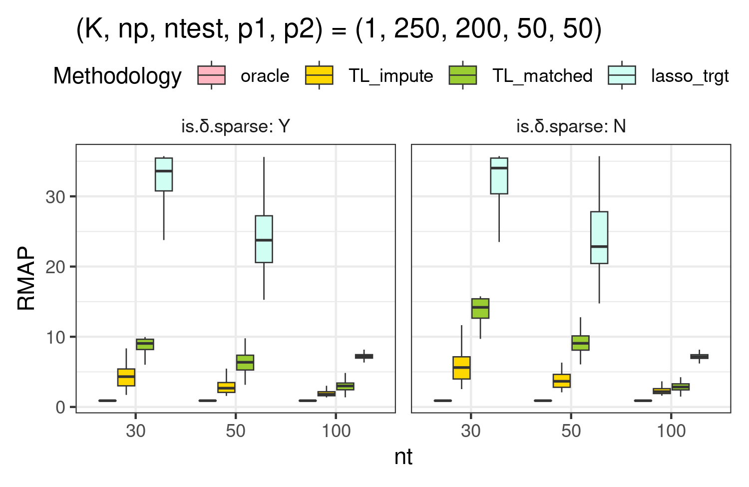
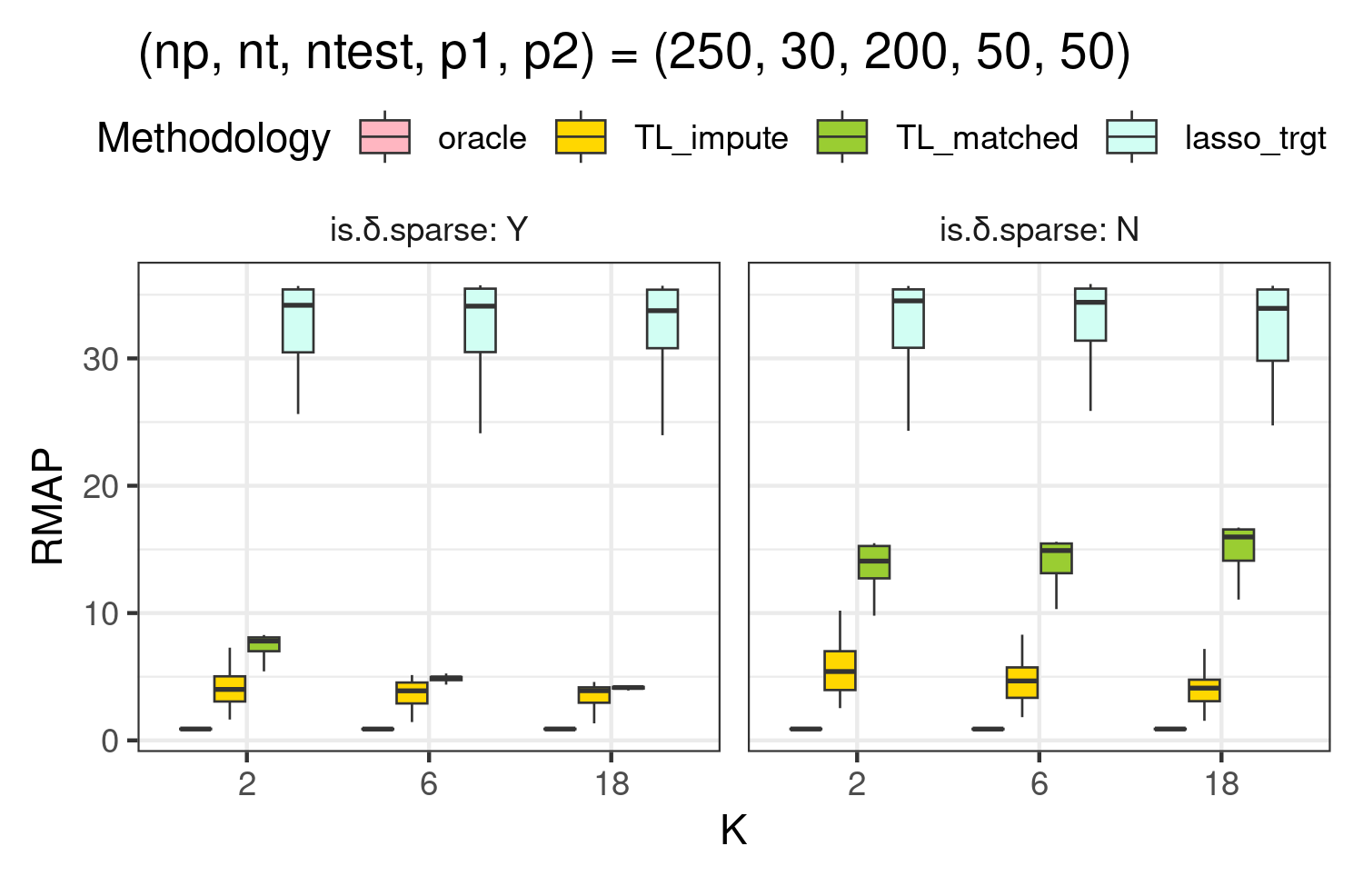
Figure 1: RMAPs of considered methodologies with sparse $\delta^{*}$ (is.$\delta$.sparse:Y) and non-sparse $\delta^{*}$ (is.$\delta$.sparse:N). In the upper row $n_{\mathfrak{t}}$ is increased keeping $K,n_{\mathfrak{p}},n_{test},p_{1},p_{2}$ fixed, while in the lower row $K$ is increased keeping $n_{\mathfrak{p}},n_{\mathfrak{t}},n_{test},p_{1},p_{2}$ fixed.

In this section, we conduct a comprehensive simulation study to understand the finite sample behavior of our HTL estimators. For generating the data, we set $\Sigma_{11,\mathfrak{p}}:=\mathbf{I}_{p_{1}}$ and take i.i.d. rows of $\mathbf{X}_{1\mathfrak{p}}^{(k)}\in\mathbb{R}^{n_{\mathfrak{p}}\times{p_{1}}}$ from $\mathcal{N}_{p_{1}}(\mathbf{o}_{p_{1}},\Sigma_{11,\mathfrak{p}})$ for each $k=1,\dots,K$, and generate $\Xi_{\mathfrak{p}}^{(k)}\in\mathbb{R}^{n_{\mathfrak{p}}\times{p_{2}}}$ from a multivariate normal distribution with mean $\mathbf{o}_{p_{2}}$ and covariance $\Sigma_{\xi\mathfrak{p}}^{(k)}=\mathbf{I}_{p_{2}}$ for $k=1,\dots,K$. For the target domain, we take ${\mathbf{X}_{1\mathfrak{t}}}\in\mathbb{R}^{{n_{\mathfrak{t}}}\times{p_{1}}}$ from $\operatorname{Uniform}(0,\sqrt{12})$ with i.i.d. coordinates so that $\Sigma_{11,\mathfrak{t}}=\mathbf{I}_{p_{1}}$. Also we take i.i.d. rows of ${\Xi_{\mathfrak{t}}}\in\mathbb{R}^{{n_{\mathfrak{t}}}\times{p_{2}}}$ from $\mathcal{N}_{p_{2}}(\mathbf{o}_{p_{2}},\mathbf{I}_{p_{2}})$. We use the same regime for generating $\mathbf{X}_{1,\text{test}},\Xi_{\text{test}}$. Thus, we assume heterogeneous distributions even for the matched features $\mathbf{X}_{1}$ between the target and proxy domain.

We take the i.i.d. entries of $\Theta_{\mathfrak{t}}$ from $10\times\operatorname{Beta}(10,10)$ distribution. Then, we obtain the entries of $\Theta_{\mathfrak{p}}^{(k)}$ by adding i.i.d. $\frac{1}{3}\left\{\operatorname{Beta}(4,4)-\frac{1}{2}\right\}$ random variables to the entries of $\Theta_{\mathfrak{t}}$ for $k=1,...,K$. Then, ${\mathbf{X}_{2\mathfrak{t}}}$ and $\mathbf{X}_{2,\text{test}}$ are sampled using the common process $\mathbf{X}_{2}=\mathbf{X}_{1}\Theta_{\mathfrak{t}}+\Xi$ while $\mathbf{X}_{2\mathfrak{p}}^{(k)}$ are taken as $\mathbf{X}_{2\mathfrak{p}}^{(k)}=\mathbf{X}_{1\mathfrak{p}}^{(k)}\Theta_{\mathfrak{p}}^{(k)}+\Xi_{\mathfrak{p}}^{(k)}$.

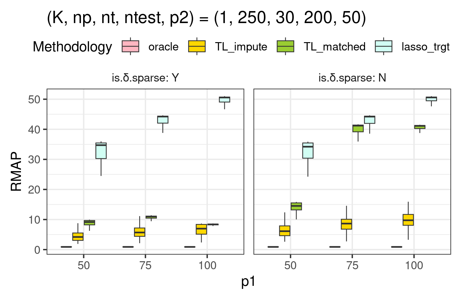
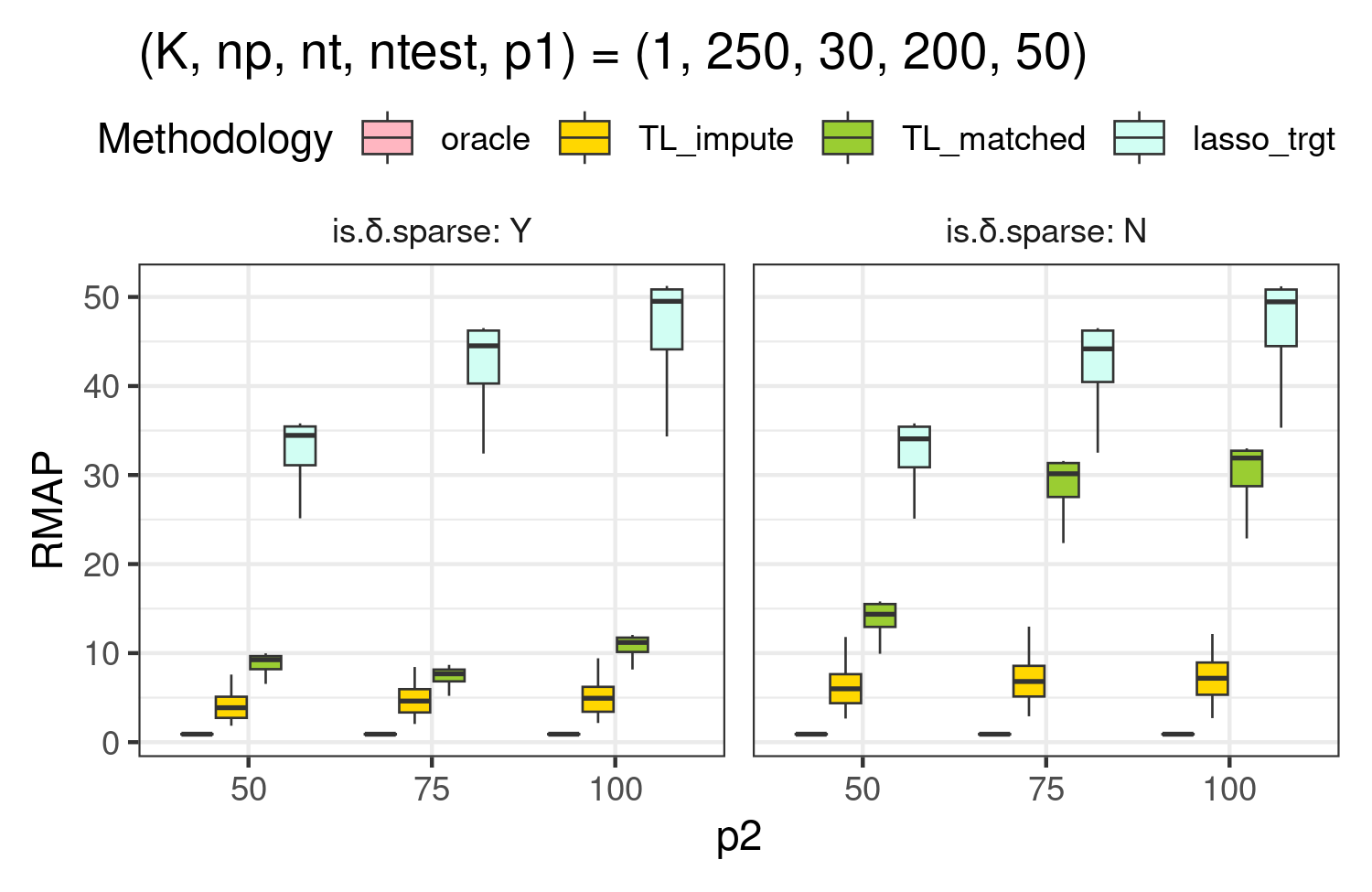
Figure 2: RMAP of considered methodologies with sparse $\delta^{*}$ and non-sparse $\delta^{*}$. In the upper row $p_{1}$ is increased keeping $K,n_{\mathfrak{p}},n_{\mathfrak{t}},n_{test},p_{2}$ fixed, while in the lower row $p_{2}$ is increased keeping $K,n_{\mathfrak{p}},n_{\mathfrak{t}},n_{test},p_{1}$ fixed.

Model errors for target and proxy domains are jointly generated from bivariate normal $\mathcal{N}_{2}\left(\mathbf{o}_{2},\begin{bmatrix}1&0.5\\ 0.5&1\end{bmatrix}\right)$ distribution and are used for generating the target and test outcomes, and the outcomes of proxy domains. We set our true target regression coefficient as $\beta_{\mathfrak{t}}^{*}=\mathbf{1}_{m}\otimes\beta$ for $\beta=(1,0,\dots,0)^{\prime}\in\mathbb{R}^{p/m}$ for $m:=(0.12)p$, so that the vector $\beta$ is repeated $m$ times. We take first ${p_{1}}$ entries as $\beta^{*}_{1\mathfrak{t}}$ and take the rest as $\beta^{*}_{2\mathfrak{t}}$. Then, our responses are generated by:

$$\mathbf{y}_{\mathfrak{p}}^{(k)} =\mathbf{X}_{\mathfrak{p}}^{(k)}\left(\beta_{\mathfrak{t}}^{*}-\delta^{*(k)}\right)+\epsilon_{\mathfrak{p}}^{(k)},~k=1,\dots,K$$

$$\mathbf{y}_{\mathfrak{t}} ={\mathbf{X}_{\mathfrak{t}}}\beta_{\mathfrak{t}}^{*}+\epsilon_{\mathfrak{t}},~\mathbf{y}_{\text{test}}=\mathbf{X}_{\text{test}}\beta_{\mathfrak{t}}^{*}+\epsilon_{\text{test}}.$$

Note that ${\mathbf{X}_{2\mathfrak{t}}}$ and $\mathbf{X}_{2,\text{test}}$ can’t be used for estimation of $\beta_{\mathfrak{t}}^{*}$ or prediction, as we assume we only observe ${\mathbf{X}_{1\mathfrak{t}}}$ and $\mathbf{X}_{1,\text{test}}$. We consider both sparse and non-sparse scenarios for $\delta_{l}^{*(k)}$, $l=1,2$. In the sparse case, we generate $\delta^{*(k)}_{lj}=C_{j}b_{lj}$ for $j=1,\dots,p_{l}$, where $C_{1},\dots,C_{p_{l}}\overset{i.i.d.}{\sim}\mathcal{N}(0,4^{-2})$ and $b_{lj}$ is randomly chosen without replacement from $\mathbf{b}_{l}=(\mathbf{1}_{S_{0}}^{\prime},{\mathbf{o}_{p_{l}-S_{0}}}^{\prime})^{\prime}$ where $S_{0}$ is the largest integer smaller than $\sqrt{p/2}$. For the non-sparse case, we take $\delta^{*}=(C_{1},\dots,C_{p})^{\prime}$.

We run 200 replications of this simulation and conduct four different types of predictions for $\mathbf{y}_{\text{test}}$ in each iteration. Oracle prediction errors are calculated by $\mathbf{y}_{\text{test}}-\mathbf{X}_{\text{test}}\beta^{*}_{\mathfrak{t}}$ which is equal to the test domain error $\epsilon_{\text{test}}$. TL_impute is our proposed method, where we calculate $\tilde{\mathbf{X}}_{\text{test}}\hat{\beta}_{\mathfrak{t}}$, with $\tilde{\mathbf{X}}_{\text{test}}$ obtained via imputation of $\mathbf{X}_{2,\text{test}}$ as $\tilde{\mathbf{X}}_{2,\text{test}}=\mathbf{X}_{1,\text{test}}\hat{\Theta}_{\mathfrak{t}}$. TL_matched prediction corresponds to the strategy in Bastani, (2021), where the mismatched target sample ${\mathbf{X}_{2\mathfrak{t}}}$ is ignored, and only matched feature effects $\beta_{1\mathfrak{t}}^{*}$ is estimated by $\hat{\beta}_{1\mathfrak{t}}^{hm}$ using ${\mathbf{X}_{1\mathfrak{t}}}$ and $\mathbf{X}_{\mathfrak{p}}$. Lasso_trgt uses lasso regression on the target domain to obtain $\hat{\beta}_{1\mathfrak{t}}^{\text{lasso}}$. Root-mean-absolute-prediction errors (RMAP) of considered methodologies are reported for comparison in Figures 1 and 2 along with the choice of $(K,n_{\mathfrak{p}},{n_{\mathfrak{t}}},n_{\rm test},{p_{1}},{p_{2}})$. We also computed prediction errors for OLS (Ordinary least squares) using proxy data alone but did not plot it as the prediction errors are too large to meaningfully compare them in the same plot with other methods. The OLS on the target data is often infeasible in some of our simulation settings due to having more predictors than sample size.

In the first two plots of Figure 1, boxplots of prediction errors are reported with increasing target sample size $n_{\mathfrak{t}}$. As expected, all of the considered methodologies show significant decrease in the prediction errors, but two transfer learning estimators–$\hat{\beta}_{\mathfrak{t}}^{ht}$ and $\hat{\beta}_{1\mathfrak{t}}^{hm}$–produce more accurate predictions than $\hat{\beta}_{1\mathfrak{t}}^{\text{lasso}}$ for all choices of ${n_{\mathfrak{t}}}=30,50,100$. Both TL methods experience elevated prediction errors when $\delta^{*}$ is not sparse compared to the opposite case. However, for smaller values of ${n_{\mathfrak{t}}}$, the performance gap between TL_impute and TL_matched is high, showing the superiority of our TL_impute approach in both sparse and non-sparse cases. This is consistent with our theoretical observations in Theorem 4.1, since the estimation error bound for HTL (and prediction error) decreases as $n_{\mathfrak{t}}$ increases. The next two plots of Figure 1 consider the case where we have more proxy studies. There is a clear gap in performance between TL methods and lasso, even when we have only two proxy studies. The greater $K$ is, the more accurate TL predictions are, and this aligns with the observations in Li et al., (2022) as well. So, the benefit of transferring knowledge is evident when we have heterogeneous features under both sparse and non-sparse discrepancy between $\beta_{\mathfrak{p}}^{*}$ and $\beta_{\mathfrak{t}}^{*}$. When $\delta^{*}$ is sparse, both TL methods appear to perform similarly when $K$ is large (e.g., $K=18$). However, the distribution of $\operatorname{RMAP}_{\text{TL\_impute}}$ suggests it serves as the lower bound for $\operatorname{RMAP}_{\text{TL\_matched}}$. Furthermore, if $\delta^{*}$ is not sparse, $\hat{\beta}_{1\mathfrak{t}}^{hm}$ is producing worse predictions in $K$ while $\hat{\beta}_{\mathfrak{t}}^{ht}$ produces significantly lower prediction errors in $K$.

Next, we examine the effect of model dimensions on the prediction errors in Figure 2. No matter the methodology or the sparsity of $\delta^{*}$, the prediction errors increase in larger ${p_{1}}$ and ${p_{2}}$. General theoretical findings also suggest that ${p_{1}}$ (plus ${p_{2}}$ according to our theory) contributes as key factor to the rise in prediction errors. Specifically, the amount of prediction accuracy loss is larger in ${p_{1}}$ compared to ${p_{2}}$, and this aligns well with our theory as the asymptotic prediction risk decomposes as the sum of $\sqrt{\log{p_{2}}}$ and $\mathcal{R}(\hat{\beta}_{\mathfrak{t}}^{ht},\beta_{\mathfrak{t}}^{*})$ scaled by $\sqrt{{p_{1}}\log{p_{1}}}$. When $\delta^{*}$ is not sparse, our approach performs the best among non-oracle methods in both larger ${p_{1}}$ and ${p_{2}}$ while $\hat{\beta}_{1\mathfrak{t}}^{hm}$ suffers from large prediction errors. When $\delta^{*}$ is sparse, our approach again achieves prediction errors that are closest to the oracle prediction errors in both large ${p_{1}}$ and ${p_{2}}$.

Next, we also consider estimation errors of the matched target feature effect $\beta_{1\mathfrak{t}}^{*}$ under the scenarios considered so far in the simulation section. The estimation errors are all measured in $\ell_{1}$-norm as $\|\hat{\beta}_{1\mathfrak{t}}-\beta_{1\mathfrak{t}}^{*}\|_{1}$ for each estimator to keep the metric the same as theoretical results.

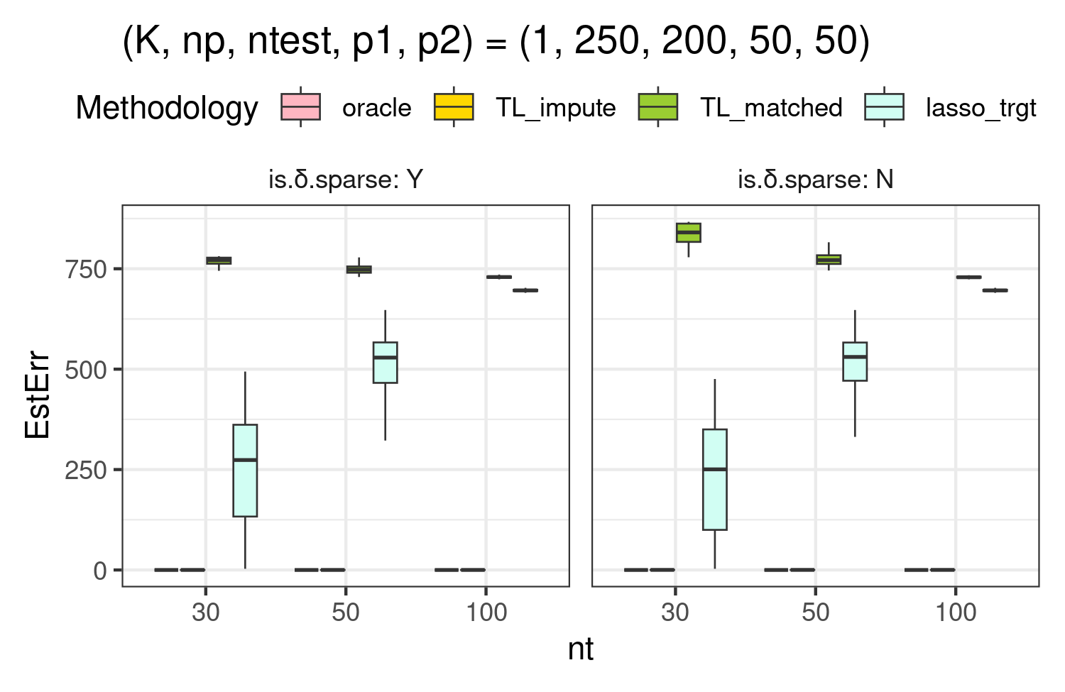
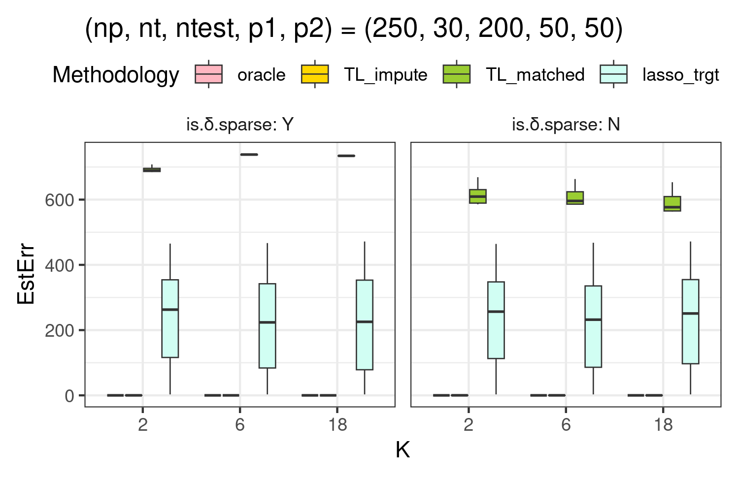
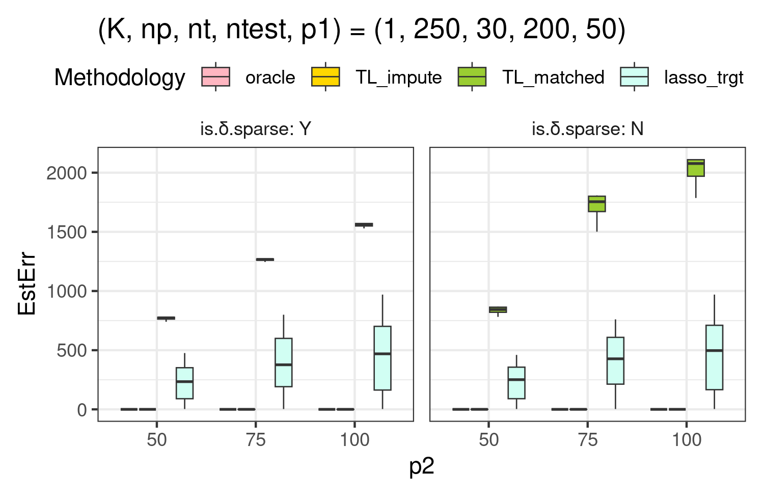
Figure 3: Estimation error of considered methodologies with sparse $\delta^{*}$ and non-sparse $\delta^{*}$, with increasing $n_{\mathfrak{t}},K,p_{1},p_{2}$ respectively. The boxplots of the errors for TL-impute are close to the Oracle and appear as horizontal lines close to 0 due to the scale of the figure.

In Figure 3, we note that when ${n_{\mathfrak{t}}}$ grows, the estimation error of $\hat{\beta}_{1\mathfrak{t}}^{\text{lasso}}$ increases while that of $\hat{\beta}_{1\mathfrak{t}}^{hm}$ shows marginal decrease, and they appear to be converging to a common point. Considering the prediction results, these indicate that both estimators are introducing a certain amount of estimation bias to improve predictions in the absence of the covariates $\mathbf{X}_{2}$. In the remaining three scenarios (increasing $K$, increasing $p_{1}$, increasing $p_{2}$), it is very clear that the TL_matched method has a large estimation error due to model misspecification introduced by ignoring $\mathbf{X}_{2}$. This is also in line with our theoretical results in Theorem 4.2, which shows the estimation error of TL_matched is of $O(|S_{1}|+\sqrt{p_{1}})$. Therefore, the estimation error does not decrease with increasing $n_{\mathfrak{t}}$ and increases with increasing $p_{1}$. These observations are evident in Figure 3. In contrast, our TL_impute method continues to provide superior estimation accuracy under all scenarios. As predicted by Theorem 4.1, the estimation error of TL_impute is much lower than that of TL-matched and lassotrgt.

Overall, the simulation results of this section substantiate the strength of HTL as it outperforms both lasso regression on target data alone and homogeneous transfer learning.

6 Case Study: Ovarian Cancer Gene Expression Data

We apply our transfer learning approach to two microarray gene expression datasets available from a curated data collection on ovarian cancer. We refer to Ganzfried et al., (2013) for details on the data collection.

Motivation. We are interested in predicting the survival time of study participants from the day of the microarray test. Prediction tasks such as the one considered here—sometimes referred to as phenotyping—are typically helpful in understanding the severity of the disease. They can inform clinical decision-making or design studies to compare alternative treatments (e.g. Loureiro et al.,, 2021; Enroth et al.,, 2022; Yang et al.,, 2024).

It is typical for a study targeting a certain population to focus on a subgroup of genes known to be correlated or predictive of a certain phenotype (e.g., survival). However, other data sources targeting different populations are also available and can be used to improve predictions (Zhao et al.,, 2022). Approaches incorporating transfer learning ideas have been considered for these prediction tasks and showed potential in empirical analysis (e.g., Zhao et al.,, 2022; Jeng et al.,, 2023). To our knowledge, most of these methods use heuristics to transfer knowledge across datasets without proper statistical formulations.

In this section, we focus on patients affected by ovarian cancer and show that our approach to transfer learning can help improve prediction compared to discarding or partially using proxy data.

Preprocessing. To mimic the practice of phenotyping, we consider two datasets from the curated ovarian cancer collection: The one presented in Tothill et al., (2008) (as target) and the one in Bonome et al., (2008) (as proxy). From now on, we will refer to these datasets only with target and proxy to simplify the exposition. From both datasets, we select patients with information on survival status: $113$ for the target and $129$ for the proxy. As a response variable, we consider the logarithm of the number of days from enrollment in the study until death. Before the analysis, we select a subsample of genes correlated with survival. In our application, we base this selection on the target and proxy data, but more general contextual knowledge or other external data should be used for this task. Specifically, we fit a lasso model on the target datasets with the smallest available tuning parameter (full-rank design matrix). Of these variables, we keep the $p_{1}=69$ common to both target and proxy. We also fit a lasso model to the proxy dataset with the smallest available lambda and use these additional $p_{2}=147$ variables as our $\mathbf{X}_{2\mathfrak{p}}$ matrix.

Prediction results. We compare the predictive performance of four models: ordinary least square (OLS) on the target data (ols_trgt), lasso on the target data (lasso_trgt), the transfer learning approach presented in Bastani, (2021) (TL_matched), and our approach TL_imputed. We used a ridge regression for the imputation step for both TL_matched and TL_imputed. The ridge parameter has been selected minimizing the prediction error in cross-validation (CV).

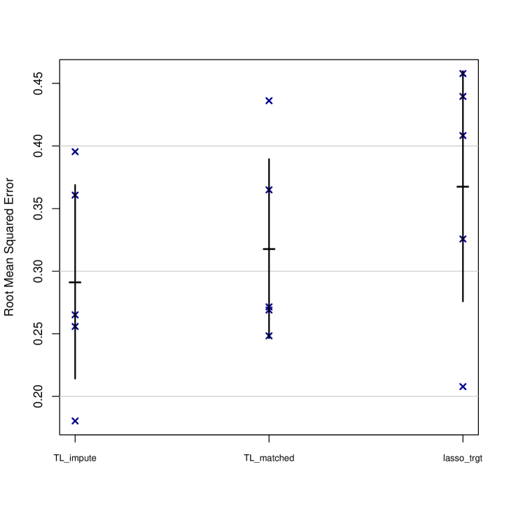
Figure 4: Root mean squared Error (RMSE) for the approaches considered in Section 6. For each method, the ‘–’ is the mean RMSE, the error bar is an approximate 95% interval for the mean RMSE, while each ‘x’ is the individual RMSE for the five-folds. The RMSE estimate for the OLS has a mean of $33.2$ with a SD of $1.95$ and has not been plotted.

To compare these four approaches, we use a CV scheme, dividing the target data into five folds and using, in turn, four to estimate our model and one to calculate the Root Mean Squared Error (RMSE). Note that the estimate of the RMSE is biased because the response variable has been used in the pre-processing of the data, but the relative comparison is still valid. The estimated CV RMSE are $33.2$ for ols_trgt, $0.38$ for lasso_trgt, $0.32$ for TL_matched and $0.29$ for TL_imputed. Figure  4 shows the results. Both TL_matched and TL_imputed improves prediction over lasso_trgt. In particular, the variance of the error estimate of the TL approach is reduced compared to lasso_trgt (and ols_trgt). Our approach provides the smallest CV error. We note that our application’s sample size for the target and proxy data are similar. Larger improvements in prediction accuracy are expected in settings where the sample size of the proxy dataset is much larger than the target.

Estimate of regression coefficients. To better understand the differences between the considered methods, we also compare the distribution of regression coefficients obtained via non-parametric bootstrap on the target data. Proxy data are fixed. Figure 5 shows the bootstrap distribution of six regression coefficients estimated using TL_imputed, TL_matched, and lasso_trgt. Although no ground truth is known, the medians of the bootstrap distributions are often similar for these three methods. For example, for the gene CD151, the median is approximately zero for all three methods. This suggests the methods have a similar central tendency in estimating the coefficients. However, because of the more extensive use of the proxy data, the variability in the coefficient estimates of TL_imputed method is typically smaller than the other approaches, suggesting a smaller standard error for the TL_imputed estimators.

Figure 5: Bootstrap distribution of six regression coefficients. OLS estimates are not plotted as their distribution substantially differs from the other methods.

7 Conclusion

In this article we have developed a method for heterogeneous transfer learning that allows missing features in the target domain and theoretically studied the estimation and prediction error from our method. This is a step towards broadening the scope of the existing statistical methods of transfer learning. In terms of knowledge transfer across domains, existing homogeneous methods assume the same set of covariates are observed across domains, limiting their practical utility, while existing heterogeneous transfer learning methods do not provide statistical error guarantees and uncertainty bounds limiting their utility for scientific discovery. Our work fills this gap by proposing methods that simultaneously are applicable to heterogeneous domains and provide rigorous statistical estimation guarantees.

Appendix A Appendix A: Additional simulation results

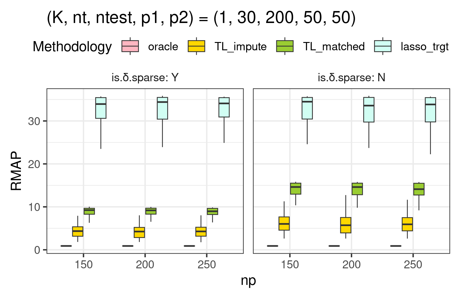
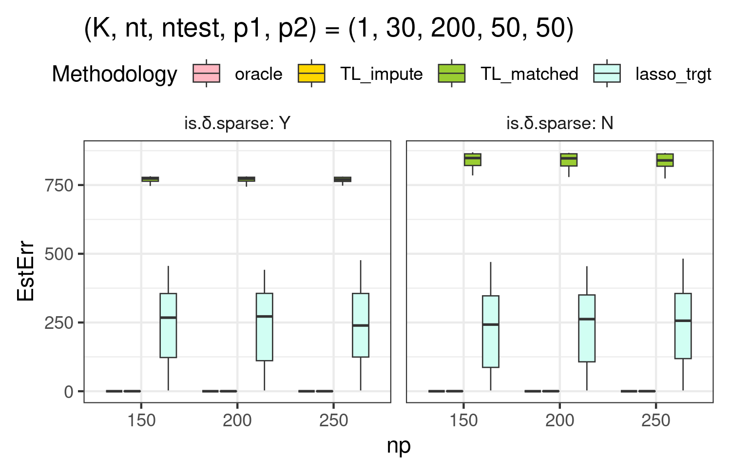
Figure 6: RMAP and estimation errors when $n_{\mathfrak{p}}$ increases

In Figure 6, we show the estimation errors measured in $l_{1}$ norm of parameters for the matched covariates and prediction errors measured in RMAP as the proxy sample size $n_{\mathfrak{p}}$ increases. Observe that prediction results do not improve with larger $n_{\mathfrak{p}}$ for both TL strategies. This is because, once enough proxy data is available for learning proxy features, the predictions on the target domain mainly benefit from the information represented by ${n_{\mathfrak{t}}}$ and $|S|$. Next, TL_matched shows much higher estimation error for $\beta_{1\mathfrak{t}}^{*}$ compared to the other methods. The estimation errors of lasso_trgt are smaller than TL_matched despite having a worse prediction error. Our TL_impute approach outperforms both TL_matched and lasso_trgt in terms of both estimation and prediction errors. Lasso is primarily designed to enhance predictions in homogeneous domains by balancing estimator bias and variance. Despite incurring higher estimation bias, the prediction results of lasso presented in the simulation section are less rewarding compared to those from our method. Therefore, we emphasize that feature map learning can even empower estimations on target tasks beside predictions.

Appendix B Appendix B: Proof of section 4.1

First, the estimation and predictions of $\hat{\beta}_{\mathfrak{t}}^{ht}$ and $\hat{\beta}_{1\mathfrak{t}}^{hm}$ with single proxy domain can be considered as special cases of transfer learning with multiple proxy studies. In this regard, we only include the proof for the case when $K\geq 1$.

Here, we prove the upper bounds of estimation risks for proposed joint estimator $\hat{\beta}_{\mathfrak{t}}^{ht}$ when there are multiple proxy datasets. Let us write $\mathbf{\cal E}_{\mathfrak{t}}=\left(\epsilon_{1,\mathfrak{t}},...,\epsilon_{{n_{\mathfrak{t}}},\mathfrak{t}}\right)^{\prime}$ to denote the target model errors and $\delta_{l}^{ht}:=\beta_{l}-\hat{\beta}_{l\mathfrak{p}}^{ht}$, $\tilde{\delta}_{l}^{ht}:=\beta_{l\mathfrak{t}}^{*}-\hat{\beta}_{l\mathfrak{p}}^{ht}$ to denote an arbitrary and true dicrepancy parameter that are approximated by proxy estimators. Also, let $\nu_{l}^{ht(k)}:=\hat{\beta}_{l\mathfrak{p}}^{ht}-\beta_{l\mathfrak{p}}^{*(k)}$ denote those approximation errors for $l=1,2$. With the imputation of ${\mathbf{X}_{2\mathfrak{t}}}$, finding $\hat{\beta}_{\mathfrak{t}}^{ht}$ is equivalent to finding $\delta^{ht}$ such that

$$\hat{\delta}^{ht} =\underset{\delta^{ht}\in\mathbb{R}^{p}}{\arg\min}\left\{\frac{1}{{n_{\mathfrak{t}}}}\left\|\mathbf{\cal E}_{\mathfrak{t}}+\sum_{l=1}^{2}\mathbf{X}_{l\mathfrak{t}}(\tilde{\delta}_{l}^{ht}-\delta_{l}^{ht})+\Delta\left(\beta_{2t}^{*}+\delta_{2}^{ht}-\tilde{\delta}_{2}^{ht}\right)\right\|^{2}+\sum_{l=1}^{2}\lambda_{l}\|\delta_{l}^{ht}\|_{1}\right\}$$ (3)

where $\Delta={\mathbf{X}_{2\mathfrak{t}}}-\hat{\mathbf{X}}_{2\mathfrak{t}}$ represents the imputation error of $\hat{\mathbf{X}}_{2\mathfrak{t}}$. Then, the proposed estimator takes the form of $\hat{\beta}_{\mathfrak{t}}^{ht}(\lambda_{1},\lambda_{2})=\hat{\beta}_{\mathfrak{p}}^{ht}+\hat{\delta}^{ht}(\lambda_{1},\lambda_{2})$. Next, let ${\tilde{\mathbf{X}}_{\mathfrak{t}}}:=\left[{\mathbf{X}_{1\mathfrak{t}}}|\hat{\mathbf{X}}_{2\mathfrak{t}}\right]$ be an imputed target design matrix. Since our objective function is convex, for $\delta^{ht}=\hat{\delta}^{ht}$ and $\delta^{ht}=\tilde{\delta}^{ht}$ we have the following:

$$\frac{1}{{n_{\mathfrak{t}}}}\left\|\mathbf{\cal E}_{\mathfrak{t}}+\Delta\beta_{2t}^{*}+\sum_{l=1}^{2}\mathbf{X}_{l\mathfrak{t}}(\tilde{\delta}^{ht}_{l}-\hat{\delta}^{ht}_{l})+\Delta\left(\hat{\delta}^{ht}_{2}-\tilde{\delta}^{ht}_{2}\right)\right\|^{2}+\sum_{l=1}^{2}\lambda_{l}\|\hat{\delta}^{ht}_{l}\|_{1}$$

$$\leq\frac{1}{{n_{\mathfrak{t}}}}\|\mathbf{\cal E}_{\mathfrak{t}}+\Delta\beta_{2t}^{*}\|^{2}+\sum_{l=1}^{2}\lambda_{l}\|\tilde{\delta}^{ht}_{l}\|_{1}.$$

Write $\tilde{\delta}^{ht}-\hat{\delta}^{ht}=\begin{bmatrix}\tilde{\delta}^{ht}_{1}-\hat{\delta}^{ht}_{1}\\ \tilde{\delta}^{ht}_{2}-\hat{\delta}^{ht}_{2}\end{bmatrix}$. Then, $\sum_{l}\mathbf{X}_{l\mathfrak{t}}(\tilde{\delta}^{ht}_{l}-\hat{\delta}^{ht}_{l})+\Delta\left(\hat{\delta}^{ht}_{2}-\tilde{\delta}^{ht}_{2}\right)={\tilde{\mathbf{X}}_{\mathfrak{t}}}(\tilde{\delta}^{ht}-\hat{\delta}^{ht})$ hence

$$\frac{1}{{n_{\mathfrak{t}}}}\|{\tilde{\mathbf{X}}_{\mathfrak{t}}}(\tilde{\delta}^{ht}-\hat{\delta}^{ht})\|^{2}+\sum_{l=1}^{2}\lambda_{l}\|\hat{\delta}^{ht}_{l}\|_{1}\leq\frac{2}{{n_{\mathfrak{t}}}}\left(\mathbf{\cal E}_{\mathfrak{t}}+\Delta\beta_{2t}^{*}\right)^{\prime}{\tilde{\mathbf{X}}_{\mathfrak{t}}}(\hat{\delta}^{ht}-\tilde{\delta}^{ht})+\sum_{l=1}^{2}\lambda_{l}\|\tilde{\delta}^{ht}_{l}\|_{1}.$$

Therefore, we have the inequality

$$\frac{1}{{n_{\mathfrak{t}}}}\|{\tilde{\mathbf{X}}_{\mathfrak{t}}}(\tilde{\delta}^{ht}-\hat{\delta}^{ht})\|^{2}+\sum_{l=1}^{2}\lambda_{l}\|\hat{\delta}^{ht}_{l}\|_{1}\leq\frac{2}{{n_{\mathfrak{t}}}}\|\left(\mathbf{\cal E}_{\mathfrak{t}}+\Delta\beta_{2t}^{*}\right)^{\prime}{\tilde{\mathbf{X}}_{\mathfrak{t}}}\|_{\infty}\|\hat{\delta}^{ht}-\tilde{\delta}^{ht}\|_{1}+\sum_{l=1}^{2}\lambda_{l}\|\tilde{\delta}^{ht}_{l}\|_{1}.$$ (4)

Compared to the case of homogeneous trasnfer learning, since we imputed the missing signal ${\mathbf{X}_{2\mathfrak{t}}}\beta^{*}_{2}$, an additional error term $\Delta$ and $\hat{\mathbf{X}}_{2t}$ need to be controlled in the theoretical analyses.

For simplicity, let us write $\nu^{ht}:=\sum_{k=1}^{K}\nu^{ht(k)}/K$. Define $\hat{\mathbf{S}}_{1\mathfrak{t}}:={{\mathbf{X}_{1\mathfrak{t}}}}^{\prime}{\mathbf{X}_{1\mathfrak{t}}}/{n_{\mathfrak{t}}}$, $t_{\mathfrak{p}}:=\frac{{p_{1}}{\sigma_{\xi\mathfrak{p}}}^{2}}{\sqrt{n_{\mathfrak{p}}^{(K)}}}$ and let $\Lambda:=\operatorname{diag}\left(\lambda_{1}\mathbf{I}_{p_{1}},\lambda_{2}\mathbf{I}_{p_{2}}\right)$ denote a diagonal matrix of two tuning parameters with ${p_{1}}$ and ${p_{2}}$ entries, respectively. Define $\tilde{\mathbf{S}}_{\mathfrak{t}}={{\tilde{\mathbf{X}}_{\mathfrak{t}}}}^{\prime}{\tilde{\mathbf{X}}_{\mathfrak{t}}}/{n_{\mathfrak{t}}}$ and $\hat{\mathbf{S}}_{\mathfrak{t}}={\mathbf{X}_{\mathfrak{t}}}^{\prime}{\mathbf{X}_{\mathfrak{t}}}/{n_{\mathfrak{t}}}$ and a quantity

$$b_{S} :=2\tau_{1\mathfrak{t}}\left(1+\theta_{\mathfrak{p}}^{(1)2}\right)+\frac{t_{\mathfrak{p}}{\sigma_{1\mathfrak{t}}}^{2}}{K\sqrt{n_{\mathfrak{p}}^{(K)}}}$$

and following events:

$$C_{ht} :=\left\{\|\mathbf{u}_{S}\|_{1}^{2}\leq\frac{|S|}{\phi^{2}}\|\mathbf{u}\|_{\Lambda^{-1}\tilde{\mathbf{S}}_{\mathfrak{t}}{\Lambda^{-1}}}^{2};\mathbf{u}\in\mathbb{R}^{p}\backslash\left\{\mathbf{o}_{p}\right\},\|\mathbf{u}_{S^{c}}\|_{1}\leq 3\|\mathbf{u}_{S}\|_{1}\right\},$$

$$W_{ht} :=\left\{\frac{2}{{n_{\mathfrak{t}}}}\|\left(\mathbf{\cal E}_{\mathfrak{t}}+\Delta\beta_{2t}^{*}\right)^{\prime}{\tilde{\mathbf{X}}_{\mathfrak{t}}}\|_{\infty}\leq\gamma_{w};\gamma_{w}>\frac{2t_{\mathfrak{p}}{\sigma_{1\mathfrak{t}}}^{2}}{K\sqrt{n_{\mathfrak{p}}^{(K)}}}b_{\beta}\right\},$$

$$S_{ht} :=\left\{\mathbf{u}^{\prime}\hat{\mathbf{S}}_{\mathfrak{t}}\mathbf{u}\leq b_{S};\mathbf{u}\in S^{p-1}\right\},$$

$$V_{ht} :=\left\{\|\nu^{ht}\|\leq\gamma_{v};\gamma_{v}>0\right\}.$$

Lemma B.1.

Let $\gamma_{w}>\frac{2t_{\mathfrak{p}}{\sigma_{1\mathfrak{t}}}^{2}}{K\sqrt{n_{\mathfrak{p}}^{(K)}}}b_{\beta}$. Then, the following hold.

1. Pick $\lambda_{1},\lambda_{2}>0$ such that $5\gamma_{w}\leq\lambda_{1}\leq\lambda_{2}$. Then, on $C_{ht},W_{ht}$, $S_{ht}$, and $V_{ht}$, $\hat{\delta}^{ht}$ satisfies

   $$\lambda_{1}\|\tilde{\delta}^{ht}-\hat{\delta}^{ht}\|_{1}\leq 1.25b_{S}{\gamma_{v}}^{2}+5\lambda_{2}\left(\sqrt{p}\gamma_{v}+\frac{\lambda_{2}|S|}{2\phi^{2}}\right).$$

2. Define $\zeta:=\left[\sigma_{\epsilon\mathfrak{t}}+\left\{{\sigma_{\xi\mathfrak{t}}}+{\sigma_{1\mathfrak{t}}}\left(\delta_{\theta}+\sqrt{6t_{\mathfrak{p}}}\right)\right\}b_{\beta}\right]{\sigma_{1\mathfrak{t}}}\left(1+\theta_{\mathfrak{p}}^{(1)}+\sqrt{6t_{\mathfrak{p}}}\right)$ and $r:=\frac{t_{\mathfrak{p}}{\sigma_{1\mathfrak{t}}}^{2}}{K\sqrt{n_{\mathfrak{p}}^{(K)}}}$. Let positive quantities $\lambda$, $n_{\mathfrak{p}}$ satisfy $10rb_{\beta}<\lambda<\frac{p{\sigma_{\mathfrak{p}}}\sigma_{\epsilon\mathfrak{p}}}{\rho_{\mathfrak{p}}^{(K)}}$. Then, we have

   $$\|\hat{\beta}_{\mathfrak{t}}^{ht}-\beta_{\mathfrak{t}}^{*}\|_{1}\leq 5\lambda\left\{\frac{{\sigma_{1\mathfrak{t}}}^{2}}{p}\left(1+\theta_{\mathfrak{p}}^{(1)2}+\frac{t_{\mathfrak{p}}}{K\sqrt{n_{\mathfrak{p}}^{(K)}}}\right)+1+\frac{|S|}{\phi^{2}}\right\}$$ (5)

   with probability at least $1-C^{\prime}\pi_{\delta^{ht}}\left(\lambda\right)$ where

   $$\pi_{\delta^{ht}}\left(\lambda\right):= \ p\left[Ke^{{p_{2}}\log 7-c\sqrt{n_{\mathfrak{p}}^{(K)}}{p_{1}}}+e^{-c{n_{\mathfrak{t}}}\min\left(g(\lambda),g(\lambda)^{2}\right)}+K\exp\left(-\frac{cn_{\mathfrak{p}}^{(K)}\lambda^{2}\rho_{\mathfrak{p}}^{(K)2}}{p^{2}{\sigma_{\mathfrak{p}}}^{2}\sigma_{\epsilon\mathfrak{p}}^{2}}\right)\right]$$

   $$+\exp\left\{-\frac{c{n_{\mathfrak{t}}}\tau_{1\mathfrak{t}}^{2}\left(1+\theta_{\mathfrak{p}}^{(1)2}\right)^{2}}{{\sigma_{1\mathfrak{t}}}^{4}\left(1+\theta_{\mathfrak{p}}^{(1)2}+6t_{\mathfrak{p}}\right)^{2}}\right\}+\exp\left\{-\frac{c{n_{\mathfrak{t}}}{\rho_{1\mathfrak{t}}}^{2}}{{\sigma_{1\mathfrak{t}}}^{4}\left(1+\theta_{\mathfrak{p}}^{(1)2}+6t_{\mathfrak{p}}\right)^{2}}\right\}$$

   $$+K\exp\left\{-\frac{cn_{\mathfrak{p}}^{(K)}}{{\sigma_{\mathfrak{p}}}^{4}}\left(\frac{1}{2}-c^{\prime}{\sigma_{\mathfrak{p}}}^{2}\sqrt{\frac{p}{n_{\mathfrak{p}}^{(K)}}}\right)^{2}\right\}.$$

   for $g(\lambda):=\frac{1}{\zeta}\left(\frac{\lambda}{5}-2rb_{\beta}\right)$.

Proof of Lemma B.1.

Note that $\sum_{l}\lambda_{l}\|\mathbf{x}_{l}\|_{1}=\|\Lambda\mathbf{x}\|_{1}$ where $\mathbf{x}:=({\mathbf{x}_{1}}^{\prime},{\mathbf{x}_{2}}^{\prime})^{\prime}\in\mathbb{R}^{p}$. Then on $W_{ht}$, by 4 we have

$$\frac{5}{{n_{\mathfrak{t}}}}\|{\tilde{\mathbf{X}}_{\mathfrak{t}}}(\tilde{\delta}^{ht}-\hat{\delta}^{ht})\|^{2}+5\|\Lambda\hat{\delta}^{ht}\|_{1}\leq\lambda_{1}\|\hat{\delta}^{ht}-\tilde{\delta}^{ht}\|_{1}+5\|\Lambda\tilde{\delta}^{ht}\|_{1}\leq\|\Lambda(\hat{\delta}^{ht}-\tilde{\delta}^{ht})\|_{1}+5\|\Lambda\tilde{\delta}^{ht}\|_{1}.$$

To invoke the compatibility condition and find the estimation error bound, we follow the logic of Bastani, (2021). Note that by $\nu^{ht}=\delta^{*}-\tilde{\delta}^{ht}$ for $\delta^{*}:=\sum_{k}\delta^{*(k)}$/K, the RHS satisfies

$$\|\Lambda(\hat{\delta}^{ht}-\tilde{\delta}^{ht})\|_{1}+5\|\Lambda\tilde{\delta}^{ht}\|_{1}=\|\Lambda(\hat{\delta}^{ht}-\delta^{*}+\nu^{ht})\|_{1}+5\|\Lambda(\delta^{*}-\nu^{ht})\|_{1}.$$

Note that $\Lambda\delta=\Lambda_{S}\delta_{S}+\Lambda_{S^{c}}\delta_{S^{c}}$ and $(\Lambda\delta)_{S}=\Lambda_{S}\delta_{S}$ (and vice versa). Then, we have following two inequalities:

$$\|\Lambda(\hat{\delta}^{ht}-\delta^{*}+\nu^{ht})\|_{1}\leq\|\Lambda_{S}(\hat{\delta}^{ht}_{S}-\delta_{S}^{*})\|_{1}+\|\Lambda_{S^{c}}\hat{\delta}^{ht}_{S^{c}}\|_{1}+\|\Lambda\nu^{ht}\|_{1}$$

and

$$\|\Lambda\hat{\delta}^{ht}\|_{1}=\|\Lambda_{S}\hat{\delta}^{ht}_{S}\|_{1}+\|\Lambda_{S^{c}}\hat{\delta}^{ht}_{S^{c}}\|_{1}\geq\|\Lambda_{S}\delta_{S}^{*}\|_{1}-\|\Lambda_{S}(\hat{\delta}^{ht}_{S}-\delta_{S}^{*})\|_{1}+\|\Lambda_{S^{c}}\hat{\delta}^{ht}_{S^{c}}\|_{1}.$$

Therefore, we have

$$\frac{5}{{n_{\mathfrak{t}}}}\|{\tilde{\mathbf{X}}_{\mathfrak{t}}}(\tilde{\delta}^{ht}-\hat{\delta}^{ht})\|^{2}+4\|\Lambda_{S^{c}}\hat{\delta}^{ht}_{S^{c}}\|_{1}\leq 6\|\Lambda_{S}(\hat{\delta}^{ht}_{S}-\delta_{S}^{*})\|_{1}+\|\Lambda\nu^{ht}\|_{1}+5\|\Lambda(\delta^{*}-\nu^{ht})\|_{1}-5\|\Lambda_{S}\delta_{S}^{*}\|_{1}$$

hence

$$\frac{5}{{n_{\mathfrak{t}}}}\|{\tilde{\mathbf{X}}_{\mathfrak{t}}}(\tilde{\delta}^{ht}-\hat{\delta}^{ht})\|^{2}+4\|\Lambda_{S^{c}}\hat{\delta}^{ht}_{S^{c}}\|_{1}\leq 6\|\Lambda_{S}(\hat{\delta}^{ht}_{S}-\delta_{S}^{*})\|_{1}+6\|\Lambda\nu^{ht}\|_{1}.$$

Next we consider the following two cases (i) and (ii).

1. First if $\|\Lambda\nu^{ht}\|_{1}\leq\|\Lambda_{S}(\hat{\delta}^{ht}_{S}-\delta_{S}^{*})\|_{1}$, we have

   $$\frac{5}{{n_{\mathfrak{t}}}}\|{\tilde{\mathbf{X}}_{\mathfrak{t}}}(\tilde{\delta}^{ht}-\hat{\delta}^{ht})\|^{2}+4\|\Lambda_{S^{c}}\hat{\delta}^{ht}_{S^{c}}\|_{1}\leq 12\|\Lambda_{S}(\hat{\delta}^{ht}_{S}-\delta_{S}^{*})\|_{1}$$

   hence for $\delta^{*}_{S^{c}}=0$, we have $\|\Lambda_{S^{c}}(\hat{\delta}^{ht}_{S^{c}}-\delta^{*}_{S^{c}})\|_{1}\leq 3\|\Lambda_{S}(\hat{\delta}^{ht}_{S}-\delta_{S}^{*})\|_{1}$. Therefore, applying the compatibility condition to $\mathbf{u}=\Lambda(\hat{\delta}^{ht}-\delta^{*})$ and $\mathbf{D}=\|\Lambda\|\Lambda^{-1}$ in Definition 4, on $C$ we have

   $$\|\Lambda_{S}(\hat{\delta}^{ht}_{S}-\delta^{*}_{S})\|_{1}^{2}\leq\frac{|S|{\lambda_{2}}^{2}}{{n_{\mathfrak{t}}}\phi^{2}}\|{\tilde{\mathbf{X}}_{\mathfrak{t}}}(\hat{\delta}^{ht}-\delta^{*})\|^{2}.$$

   Next,

   $$\frac{5}{{n_{\mathfrak{t}}}} \|{\tilde{\mathbf{X}}_{\mathfrak{t}}}(\tilde{\delta}^{ht}-\hat{\delta}^{ht})\|^{2}+4\|\Lambda(\tilde{\delta}^{ht}-\hat{\delta}^{ht})\|_{1}$$

   $$\leq\frac{5}{{n_{\mathfrak{t}}}}\|{\tilde{\mathbf{X}}_{\mathfrak{t}}}(\tilde{\delta}^{ht}-\hat{\delta}^{ht})\|^{2}+4\left(\|\Lambda_{S}(\hat{\delta}^{ht}_{S}-\delta^{*}_{S})\|_{1}+\|\Lambda_{S^{c}}\hat{\delta}^{ht}_{S^{c}}\|_{1}+\|\Lambda\nu^{ht}\|_{1}\right)$$

   $$\leq 10\left(\|\Lambda_{S}(\hat{\delta}^{ht}_{S}-\delta_{S}^{*})\|_{1}+\|\Lambda\nu^{ht}\|_{1}\right)$$

   by the previous arguments. Therefore, we get

   $$\frac{5}{{n_{\mathfrak{t}}}}\|{\tilde{\mathbf{X}}_{\mathfrak{t}}}(\tilde{\delta}^{ht}-\hat{\delta}^{ht})\|^{2}+ 4\|\Lambda(\tilde{\delta}^{ht}-\hat{\delta}^{ht})\|_{1}\leq\frac{10\lambda_{2}|S|^{1/2}}{\sqrt{{n_{\mathfrak{t}}}}\phi}\|{\tilde{\mathbf{X}}_{\mathfrak{t}}}(\hat{\delta}^{ht}-\delta^{*})\|+10\|\Lambda\nu^{ht}\|_{1}$$

   $$\leq\frac{5}{2{n_{\mathfrak{t}}}}\|{\tilde{\mathbf{X}}_{\mathfrak{t}}}(\hat{\delta}^{ht}-\delta^{*})\|^{2}+10\|\Lambda\nu^{ht}\|_{1}+\frac{10{\lambda_{2}}^{2}|S|}{\phi^{2}}$$

   $$\leq\frac{5}{{n_{\mathfrak{t}}}}\|{\tilde{\mathbf{X}}_{\mathfrak{t}}}(\hat{\delta}^{ht}-\tilde{\delta}^{ht})\|^{2}+\frac{5}{{n_{\mathfrak{t}}}}\|{\tilde{\mathbf{X}}_{\mathfrak{t}}}\nu^{ht}\|^{2}+10\|\Lambda\nu^{ht}\|_{1}+\frac{10{\lambda_{2}}^{2}|S|}{\phi^{2}}$$

   hence

   $$\|\Lambda(\tilde{\delta}^{ht}-\hat{\delta}^{ht})\|_{1}\leq\frac{5}{4}\|\nu^{ht}\|_{\tilde{\mathbf{S}}_{\mathfrak{t}}}^{2}+\frac{5}{2}\|\Lambda\nu^{ht}\|_{1}+\frac{5{\lambda_{2}}^{2}|S|}{2\phi^{2}}.$$

2. When $\|\Lambda\nu^{ht}\|_{1}\geq\|\Lambda_{S}(\hat{\delta}^{ht}_{S}-\delta_{S}^{*})\|_{1}$, then

   $$\frac{5}{{n_{\mathfrak{t}}}}\|{\tilde{\mathbf{X}}_{\mathfrak{t}}}(\tilde{\delta}^{ht}-\hat{\delta}^{ht})\|^{2}+4\|\Lambda_{S^{c}}\hat{\delta}^{ht}_{S^{c}}\|_{1}\leq 12\|\Lambda\nu^{ht}\|_{1}$$

   and

   $$\frac{5}{{n_{\mathfrak{t}}}}\|{\tilde{\mathbf{X}}_{\mathfrak{t}}}(\tilde{\delta}^{ht}-\hat{\delta}^{ht})\|^{2}+4\|\Lambda(\tilde{\delta}^{ht}-\hat{\delta}^{ht})\|_{1}\leq \frac{5}{{n_{\mathfrak{t}}}}\|{\tilde{\mathbf{X}}_{\mathfrak{t}}}(\tilde{\delta}^{ht}-\hat{\delta}^{ht})\|^{2}+4\|\Lambda_{S}(\hat{\delta}^{ht}_{S}-\delta_{S}^{*})\|_{1}+4\|\Lambda_{S^{c}}\hat{\delta}^{ht}_{S^{c}}\|_{1}$$

   $$+4\|\Lambda\nu^{ht}\|_{1}\leq 20\|\Lambda\nu^{ht}\|_{1}.$$

   Therefore, $\frac{5}{4}\|\hat{\delta}^{ht}-\tilde{\delta}^{ht}\|_{\tilde{\mathbf{S}}_{\mathfrak{t}}}^{2}+\|\Lambda(\tilde{\delta}^{ht}-\hat{\delta}^{ht})\|_{1}\leq 5\|\Lambda\nu^{ht}\|_{1}$ hence $\|\Lambda(\tilde{\delta}^{ht}-\hat{\delta}^{ht})\|_{1}\leq 5\|\Lambda\nu^{ht}\|_{1}$.

Combining the results, we get

$$\lambda_{1}\|\tilde{\delta}^{ht}-\hat{\delta}^{ht}\|_{1}\leq 1.25\,\frac{\nu^{ht\intercal}\hat{\mathbf{S}}_{\mathfrak{t}}\nu^{ht}}{\|\nu^{ht}\|^{2}}\,\|\nu^{ht}\|^{2}+5\lambda_{2}\left(\|\nu^{ht}\|_{1}+\frac{\lambda_{2}|S|}{2\phi^{2}}\right).$$ (6)

Therefore, on events $W_{ht},S_{ht},V_{ht},$ and $C_{ht}$, we can derive the conclusion. Selecting $\gamma_{w}=\lambda/5$ and $\lambda_{2}=\lambda_{1}=\lambda$, on events $C_{ht},W_{ht},S_{ht}$, and $V_{ht}$ 6 gives

$$\frac{1}{5}\|\tilde{\delta}^{ht}-\hat{\delta}^{ht}\|_{1} \leq\frac{\left\{2\left(1+\theta_{\mathfrak{p}}^{(1)2}\right)+\frac{t_{\mathfrak{p}}}{K\sqrt{n_{\mathfrak{p}}^{(K)}}}\right\}{\sigma_{1\mathfrak{t}}}^{2}{\gamma_{v}}^{2}}{4\lambda}+\sqrt{p}\gamma_{v}+\frac{\lambda|S|}{2\phi^{2}}$$

$$\leq\frac{\left(1+\theta_{\mathfrak{p}}^{(1)2}+\frac{t_{\mathfrak{p}}}{K\sqrt{n_{\mathfrak{p}}^{(K)}}}\right){\sigma_{1\mathfrak{t}}}^{2}{\gamma_{v}}^{2}}{\lambda}+\sqrt{p}\gamma_{v}+\frac{\lambda|S|}{\phi^{2}}$$

with probability at least

$$1-p\left\{C\cdot\pi_{\mathbf{E}_{\mathfrak{p}}}+\pi_{W_{ht}}(\lambda/5)+K\pi_{V_{ht}}(\gamma_{v})\right\}-\pi_{S_{ht}}(\rho_{1\mathfrak{t}}/2)-\pi_{S_{ht}}\left\{\tau_{1\mathfrak{t}}\left(1+\theta_{\mathfrak{p}}^{(1)2}\right)\right\}-K\pi_{\mathbf{X}_{\mathfrak{p}}}$$

by non-asymptotic results in appendix. Choosing $\gamma_{v}=\lambda/\sqrt{p}$ and given constrained $\lambda$, we get the estimation error upper bound in the second statement. ∎

Proof of Theorem 4.1.

Now suppose that the population variance proxies $\sigma_{\epsilon\mathfrak{t}},{\sigma_{\xi\mathfrak{t}}}$, and ${\sigma_{\xi\mathfrak{p}}}$ are all finite and non-vanishing. Then, by simple algebra we have

$$\zeta=\mathcal{O}\left(\frac{{p_{1}}}{\sqrt{n_{\mathfrak{p}}^{(K)}}}\right)\text{ and }2rb_{\beta}=c_{r}\frac{{p_{1}}}{Kn_{\mathfrak{p}}^{(K)}}$$

for some positive constant $c_{r}<\infty$. Then, since

$$\frac{1}{p}\left(1+\frac{t_{\mathfrak{p}}}{K\sqrt{n_{\mathfrak{p}}^{(K)}}}\right)+1+\frac{|S|}{\phi^{2}}\lesssim\frac{1}{Kn_{\mathfrak{p}}^{(K)}}+1+\frac{|S|}{\phi^{2}}\lesssim|S|,$$

5 gives

$$\left\|\hat{\beta}_{\mathfrak{t}}^{ht}(\lambda)-\beta^{*}_{\mathfrak{t}}\right\|_{1}\gtrsim\lambda|S|$$

with probability less than

$$Kp\exp\left({p_{2}}-c\sqrt{n_{\mathfrak{p}}^{(K)}}{p_{1}}\right)+K\exp\left\{-cn_{\mathfrak{p}}^{(K)}\left(\frac{1}{2}-\sqrt{\frac{p}{n_{\mathfrak{p}}^{(K)}}}\right)^{2}\right\}$$

$$+\exp\left\{\log p-c{n_{\mathfrak{t}}}\min\left(\frac{\sqrt{n_{\mathfrak{p}}^{(K)}}}{{p_{1}}}\left(\lambda-\frac{{p_{1}}}{Kn_{\mathfrak{p}}^{(K)}}\right),\frac{n_{\mathfrak{p}}^{(K)}}{{{p_{1}}}^{2}}\left(\lambda-\frac{{p_{1}}}{Kn_{\mathfrak{p}}^{(K)}}\right)^{2}\right)\right\}$$

$$+\exp\left(\log Kp-c\frac{n_{\mathfrak{p}}^{(K)}\lambda^{2}}{p^{2}}\right)+\exp\left(-c\frac{{n_{\mathfrak{t}}}n_{\mathfrak{p}}^{(K)}{\rho_{1\mathfrak{t}}}^{2}}{{p_{1}}^{2}}\right)$$

multiplied by a positive constant. Next, for $a\in(0,1)$ picking

$$\lambda=\max\left(\sqrt{\frac{p^{2}(\log Kp)^{1+a}}{n_{\mathfrak{p}}^{(K)}}},\frac{\log p}{{n_{\mathfrak{t}}}}\right),$$

we have $\lambda-\frac{{p_{1}}}{Kn_{\mathfrak{p}}^{(K)}}\asymp\lambda$ hence

$${n_{\mathfrak{t}}} \min\left\{\frac{\sqrt{n_{\mathfrak{p}}^{(K)}}}{{p_{1}}}\left(\lambda-\frac{{p_{1}}}{Kn_{\mathfrak{p}}^{(K)}}\right),\frac{n_{\mathfrak{p}}^{(K)}}{{{p_{1}}}^{2}}\left(\lambda-\frac{{p_{1}}}{Kn_{\mathfrak{p}}^{(K)}}\right)^{2}\right\}$$

$$=\omega\left\{\min\left(\sqrt{n_{\mathfrak{p}}^{(K)}}\frac{\log p}{{p_{1}}},{n_{\mathfrak{t}}}(\log Kp)^{1+a}\right)\right\},$$

$$\frac{n_{\mathfrak{p}}^{(K)}\lambda^{2}}{p^{2}} =\omega\left(\log Kp\right).$$

Now, assume that $n_{\mathfrak{p}}^{(K)}\asymp p^{2}(\log Kp)^{2}$. Then, we obtain

$$\|\hat{\beta}_{\mathfrak{t}}^{ht}-\beta_{\mathfrak{t}}^{*}\|_{1}=\mathcal{O}\left\{|S|\max\left(\frac{1}{\sqrt{(\log Kp)^{1-a}}},\frac{\log p}{{n_{\mathfrak{t}}}}\right)\right\}$$

with probability at least

$$1-\exp\left\{-c^{\prime}{n_{\mathfrak{t}}}p^{2}{\rho_{1\mathfrak{t}}}^{2}(\log Kp)^{2}/{p_{1}}^{2}\right\}-o(1).$$

Next define an event $\mathcal{U}_{ht}:=C_{ht}\cap W_{ht}\cap S_{ht}\cap V_{ht}$ and denote the upper bound in 5 by $w_{ht}$. This gives the expression $\left\|\hat{\beta}_{\mathfrak{t}}^{ht}(\lambda)-\beta_{\mathfrak{t}}^{*}\right\|_{1}1_{\mathcal{U}}\leq w_{ht}1_{\mathcal{U}}$ almost surely as we have just verified. The rest of the proof follows the same steps in the proof of Theorem 4.2. Therefore, we get $\mathbb{E}\left\|\hat{\beta}_{\mathfrak{t},tr}^{ht}(\lambda)-\beta_{\mathfrak{t}}^{*}\right\|_{1}\leq w_{ht}+3b_{\beta}\pi_{\delta^{ht}}(\lambda)$ and by similar arguments we can derive that

$$\mathcal{R}\left(\hat{\beta}_{\mathfrak{t},tr}^{ht},\beta^{*}_{\mathfrak{t}}\right)=\mathcal{O} \left[|S|\max\left(\frac{1}{\sqrt{(\log Kp)^{1-a}}},\frac{\log p}{{n_{\mathfrak{t}}}}\right)+\exp\left(-c^{\prime}{n_{\mathfrak{t}}}{\rho_{1\mathfrak{t}}}^{2}\frac{p^{2}(\log Kp)^{2}}{{p_{1}}^{2}}\right)\right].$$

∎

Proof of Theorem 4.3.

First, since $y_{\mathfrak{t},\text{new}}={\mathbf{x}_{\mathfrak{t},\text{new}}}\,^{\prime}\beta_{\mathfrak{t}}^{*}+\epsilon_{\mathfrak{t},\text{new}}$,

$$\left|y_{\mathfrak{t},\text{new}}-{\tilde{\mathbf{x}}_{\mathfrak{t},\text{new}}}\,^{\prime}\hat{\beta}_{\mathfrak{t},tr}^{ht}\right|\leq\left|{\mathbf{x}_{\mathfrak{t},\text{new}}}\,^{\prime}\beta_{\mathfrak{t}}^{*}-{\tilde{\mathbf{x}}_{\mathfrak{t},\text{new}}}\,^{\prime}\hat{\beta}_{\mathfrak{t},tr}^{ht}\right|+\left|\epsilon_{\mathfrak{t},\text{new}}\right|$$

and

$$\left|{\mathbf{x}_{\mathfrak{t},\text{new}}}\,^{\prime}\beta_{\mathfrak{t}}^{*}-{\tilde{\mathbf{x}}_{\mathfrak{t},\text{new}}}\,^{\prime}\hat{\beta}_{\mathfrak{t},tr}^{ht}\right| \leq\left|{\mathbf{x}_{\mathfrak{t},\text{new}}}\,^{\prime}\beta_{\mathfrak{t}}^{*}-{\tilde{\mathbf{x}}_{\mathfrak{t},\text{new}}}\,^{\prime}\beta^{*}_{\mathfrak{t}}\right|+\left|{\tilde{\mathbf{x}}_{\mathfrak{t},\text{new}}}\,^{\prime}\beta^{*}_{\mathfrak{t}}-{\tilde{\mathbf{x}}_{\mathfrak{t},\text{new}}}\,^{\prime}\hat{\beta}_{\mathfrak{t},tr}^{ht}\right|$$

$$\leq\|\mathbf{x}_{2\mathfrak{t},\text{new}}-\tilde{\mathbf{x}}_{2\mathfrak{t},\text{new}}\|_{\infty}b_{\beta}+\left|{\tilde{\mathbf{x}}_{\mathfrak{t},\text{new}}}\,^{\prime}\left(\hat{\beta}_{\mathfrak{t},tr}^{ht}-\beta_{\mathfrak{t}}^{*}\right)\right|$$

hence the prediction error depends on (beside an irreducible error $\epsilon_{\mathfrak{t},\text{new}}$) both the imputation error of mismatched sample and the estimation error of regression parameters. We know that for all $u>0$

$$\mathbb{P}\left(\left|\epsilon_{\mathfrak{t},\text{new}}\right|>u\right)<2\exp\left(-\frac{cu^{2}}{\sigma_{\epsilon\mathfrak{t}}^{2}}\right)\text{ hence }\mathbb{E}\left|\epsilon_{\mathfrak{t},\text{new}}\right|\lesssim\sigma_{\epsilon\mathfrak{t}}$$

and $\mathbf{x}_{2\mathfrak{t},\text{new}}-\tilde{\mathbf{x}}_{2\mathfrak{t},\text{new}}=\xi_{\mathfrak{t}}+\left(\Theta_{\mathfrak{t}}-\bar{\Theta}_{\mathfrak{p}}-\mathbf{E}_{\mathfrak{p}}\right)^{\prime}\mathbf{x}_{1\mathfrak{t},\text{new}}$ hence $\mathbf{x}_{2\mathfrak{t},\text{new}}-\tilde{\mathbf{x}}_{2\mathfrak{t},\text{new}}$ is conditionally sub-gaussian with variance proxy ${\sigma_{\xi\mathfrak{t}}}+\left(\delta_{\theta}+\|\mathbf{E}_{\mathfrak{p}}\|\right){\sigma_{1\mathfrak{t}}}$ given $\mathcal{F}:=\sigma\left(\mathbf{X}_{1\mathfrak{p}}^{(k)},\Xi_{\mathfrak{p}}^{(k)};k=1,\dots,K\right)$. So, by Vershynin, (2018)

$$\mathbb{E}\left(\|\mathbf{x}_{2\mathfrak{t},\text{new}}-\tilde{\mathbf{x}}_{2\mathfrak{t},\text{new}}\|_{\infty}|\mathcal{F}\right)\lesssim\left\{{\sigma_{\xi\mathfrak{t}}}+\left(\delta_{\theta}+\|\mathbf{E}_{\mathfrak{p}}\|\right){\sigma_{1\mathfrak{t}}}\right\}\sqrt{\log 2{p_{2}}}.$$

We know that

$$\mathbb{E}\|\mathbf{E}_{\mathfrak{p}}\| \leq\mathbb{E}\|\mathbf{E}_{\mathfrak{p}}\|_{F}=\mathbb{E}\sqrt{\frac{1}{K^{2}}\sum_{1\leq k,j\leq K}\frac{1}{n_{\mathfrak{p}}^{(k)}n_{\mathfrak{p}}^{(j)}}\operatorname{tr}\left(\Xi_{\mathfrak{p}}^{(k)}\,{}^{\prime}\mathbf{X}_{1\mathfrak{p}}^{(k)}\mathbf{X}_{1\mathfrak{p}}^{(j)}\,{}^{\prime}\Xi_{\mathfrak{p}}^{(j)}\right)}$$

$$\leq\frac{1}{K}\sqrt{\sum_{k}\frac{1}{n_{\mathfrak{p}}^{(k)2}}\operatorname{tr}\left(\mathbb{E}\mathbf{X}_{1\mathfrak{p}}^{(k)}\mathbf{X}_{1\mathfrak{p}}^{(k)}\,{}^{\prime}\Xi_{\mathfrak{p}}^{(k)}\Xi_{\mathfrak{p}}^{(k)}\,{}^{\prime}\right)}$$

$$=\frac{1}{K}\sqrt{\sum_{k}\frac{1}{n_{\mathfrak{p}}^{(k)2}}\operatorname{tr}\left\{\operatorname{tr}\left(\Sigma_{1\mathfrak{p}}^{(k)}\right)\operatorname{tr}\left(\Sigma_{\xi\mathfrak{p}}^{(k)}\right)\mathbf{I}_{n_{\mathfrak{p}}^{(k)}}\right\}}$$

$$\leq\frac{1}{K}\sqrt{\sum_{k}\frac{{p_{1}}{p_{2}}{\sigma_{1\mathfrak{p}}}^{2}{\sigma_{\xi\mathfrak{p}}}^{2}}{n_{\mathfrak{p}}^{(k)}}}$$

by Jensen’s inequality. So,

$$\mathbb{E}\|\mathbf{x}_{2\mathfrak{t},\text{new}}-\tilde{\mathbf{x}}_{2\mathfrak{t},\text{new}}\|_{\infty} \lesssim\left({\sigma_{\xi\mathfrak{t}}}+\delta_{\theta}{\sigma_{1\mathfrak{t}}}+\sqrt{\frac{{p_{1}}{p_{2}}{\sigma_{1\mathfrak{p}}}^{2}{\sigma_{\xi\mathfrak{p}}}^{2}}{Kn_{\mathfrak{p}}^{(K)}}}{\sigma_{1\mathfrak{t}}}\right)\sqrt{\log 2{p_{2}}}$$

$$\asymp\sqrt{\log{p_{2}}}+\mathcal{O}\left(\frac{1}{\sqrt{K\log Kp}}\right)=\mathcal{O}(\sqrt{\log{p_{2}}}).$$

Notice that $\hat{\beta}_{\mathfrak{t},tr}^{ht}$ is independent with the new observation $\mathbf{x}_{1\mathfrak{t},\text{new}}$ and dependent with $\hat{\Theta}_{\mathfrak{p}}$ for ${\tilde{\mathbf{x}}_{\mathfrak{t},\text{new}}}\,^{\prime}={\mathbf{x}_{1\mathfrak{t},\text{new}}}\,^{\prime}\left[\mathbf{I}_{p_{1}}|\hat{\Theta}_{\mathfrak{p}}\right]$. So,

$$\mathbb{E}\left|{\tilde{\mathbf{x}}_{\mathfrak{t},\text{new}}}\,^{\prime}\left(\hat{\beta}_{\mathfrak{t},tr}^{ht}-\beta_{\mathfrak{t}}^{*}\right)\right| =\mathbb{E}\left|{\mathbf{x}_{1\mathfrak{t},\text{new}}}\,^{\prime}\left[\mathbf{I}_{p_{1}}|\hat{\Theta}_{\mathfrak{p}}\right]\left(\hat{\beta}_{\mathfrak{t},tr}^{ht}-\beta_{\mathfrak{t}}^{*}\right)\right|$$

$$\leq\mathbb{E}\|\mathbf{x}_{1\mathfrak{t},\text{new}}\|_{\infty}\mathbb{E}\left[\max\left(1,\|\hat{\Theta}_{\mathfrak{p}}\|_{1}\right)\|\hat{\beta}_{\mathfrak{t},tr}^{ht}-\beta_{\mathfrak{t}}^{*}\|_{1}\right].$$

Likewise, we have

$$\mathbb{E}\|\mathbf{x}_{1\mathfrak{t},\text{new}}\|_{\infty}\lesssim{\sigma_{1\mathfrak{t}}}\sqrt{\log 2{p_{1}}}\asymp\sqrt{\log{p_{1}}}.$$

Define an event $A:=\left\{1<\|\hat{\Theta}_{\mathfrak{p}}\|_{1}\right\}$. Then,

$$\mathbb{E}\left[\max\left(1,\|\hat{\Theta}_{\mathfrak{p}}\|_{1}\right)\|\hat{\beta}_{\mathfrak{t},tr}^{ht}-\beta_{\mathfrak{t}}^{*}\|_{1}\right]<\ \mathbb{E}\left(1_{A^{c}}\|\hat{\beta}_{\mathfrak{t},tr}^{ht}-\beta_{\mathfrak{t}}^{*}\|_{1}\right)+\mathbb{E}\left[\|\hat{\Theta}_{\mathfrak{p}}\|_{1}1_{A}\|\hat{\beta}_{\mathfrak{t},tr}^{ht}-\beta_{\mathfrak{t}}^{*}\|_{1}\right].$$

By Cauchy-Schwarz inequality, we have

$$\mathbb{E}\left[\|\hat{\Theta}_{\mathfrak{p}}\|_{1}1_{A}\|\hat{\beta}_{\mathfrak{t},tr}^{ht}-\beta_{\mathfrak{t}}^{*}\|_{1}\right]\leq\left(\mathbb{E}\|\hat{\Theta}_{\mathfrak{p}}\|_{1}^{2}\mathbb{E}\|\hat{\beta}_{\mathfrak{t},tr}^{ht}-\beta_{\mathfrak{t}}^{*}\|_{1}^{2}\right)^{1/2}.$$

Then we note

$$\mathbb{E}\|\hat{\Theta}_{\mathfrak{p}}\|_{1}^{2}\leq{p_{1}}\mathbb{E}\|\hat{\Theta}_{\mathfrak{p}}\|^{2}\leq{p_{1}}\left(2\theta_{\mathfrak{p}}^{(1)2}+2\mathbb{E}\|\mathbf{E}_{\mathfrak{p}}\|^{2}\right)$$

where

$$\mathbb{E}\|\mathbf{E}_{\mathfrak{p}}\|^{2}\leq\mathbb{E}\|\mathbf{E}_{\mathfrak{p}}\|_{F}^{2}\leq\frac{{p_{1}}{p_{2}}{\sigma_{1\mathfrak{p}}}^{2}{\sigma_{\xi\mathfrak{p}}}^{2}}{Kn_{\mathfrak{p}}^{(K)}}=\mathcal{O}\left(\frac{1}{K(\log Kp)^{2}}\right)$$

hence $\mathbb{E}\|\hat{\Theta}_{\mathfrak{p}}\|_{1}^{2}=\mathcal{O}({p_{1}})$.

Next, recall by 5 we have

$$\|\tilde{\delta}^{ht}-\hat{\delta}^{ht}\|_{1}^{2}\lesssim\lambda^{2}\left\{\frac{{\sigma_{1\mathfrak{t}}}^{4}}{p^{2}}\left(1+\theta_{\mathfrak{p}}^{(1)4}+\frac{{t_{\mathfrak{p}}}^{2}}{K^{2}n_{\mathfrak{p}}^{(K)}}\right)+1+\frac{|S|^{2}}{\phi^{4}}\right\}=:w_{ht}$$

with probability at least $1-c\cdot\pi_{\delta^{ht}}\left(\lambda\right)$. By the same choice of $\lambda$ and similar arguments as in the proof of Theorem 4.1, it is straightforward to derive that

$$\mathbb{E}\left\|\hat{\beta}_{\mathfrak{t},tr}^{ht}-\beta_{\mathfrak{t}}^{*}\right\|_{1}^{2}\lesssim w_{ht}+\pi_{\delta^{ht}}.$$

Therefore, if $n_{\mathfrak{p}}^{(K)}=\Omega\left\{p^{2}(\log Kp)^{2}\right\}$, we can easily derive that

$$\mathbb{E}\|\hat{\beta}_{\mathfrak{t},tr}^{ht}-\beta_{\mathfrak{t}}^{*}\|_{1}^{2}=\mathcal{O}\left[|S|^{2}\left(\frac{1}{(\log Kp)^{1-a}}+\frac{\log^{2}p}{{n_{\mathfrak{t}}}^{2}}\right)+\exp\left(-c^{\prime}{n_{\mathfrak{t}}}{\rho_{1\mathfrak{t}}}^{2}\frac{p^{2}(\log Kp)^{2}}{{p_{1}}^{2}}\right)\right]$$

$$\asymp\mathcal{R}(\hat{\beta}_{\mathfrak{t},tr}^{ht},\beta_{\mathfrak{t}}^{*})^{2}.$$

In summary, we have

$$\mathbb{E}\left|{\tilde{\mathbf{x}}_{\mathfrak{t},\text{new}}}\,^{\prime}\left(\hat{\beta}_{\mathfrak{t},tr}^{ht}-\beta_{\mathfrak{t}}^{*}\right)\right|\asymp\sqrt{\log{p_{1}}}\left[\mathcal{R}(\hat{\beta}_{\mathfrak{t},tr}^{ht},\beta_{\mathfrak{t}}^{*})+\sqrt{{p_{1}}}\left(\mathbb{E}\|\hat{\beta}_{\mathfrak{t},tr}^{ht}-\beta_{\mathfrak{t}}^{*}\|_{1}^{2}\right)^{1/2}\right]$$

$$\asymp\sqrt{{p_{1}}\log{p_{1}}}\mathcal{R}(\hat{\beta}_{\mathfrak{t},tr}^{ht},\beta_{\mathfrak{t}}^{*}).$$

This completes the proof. ∎

Appendix C Estimation in homogeneous transfer learning

Here we work on the estimation error for homogeneous transfer learning in Bastani, (2021) under our model and problem setup. Following the same framework of section 4.1, if we take $\delta_{1}^{hm}=\beta_{1}-\hat{\beta}_{1\mathfrak{p}}^{hm}$ and $\mathbf{\cal E}_{\mathfrak{t}}=\left(\epsilon_{1,\mathfrak{t}},...,\epsilon_{{n_{\mathfrak{t}}},\mathfrak{t}}\right)^{\prime}$, finding $\hat{\beta}_{1\mathfrak{t}}^{hm}$ is equivalent to finding

$$\hat{\delta}_{1}^{hm} =\underset{\delta_{1}^{hm}\in\mathbb{R}^{{p_{1}}}}{\arg\min}\left\{\frac{1}{{n_{\mathfrak{t}}}}\left\|\mathbf{y}_{\mathfrak{t}}-\mathbf{X}_{1\mathfrak{t}}\left(\delta_{1}^{hm}+\hat{\beta}_{1\mathfrak{p}}^{hm}\right)\right\|^{2}+\lambda_{1}\|\delta_{1}^{hm}\|_{1}\right\}$$

$$={\arg\min}_{\delta_{1}^{hm}}\left\{\frac{1}{{n_{\mathfrak{t}}}}\left\|\mathbf{X}_{1\mathfrak{t}}(\tilde{\delta}_{1}^{hm}-\delta_{1}^{hm})+{\mathbf{X}_{2\mathfrak{t}}}\beta_{2t}^{*}+\mathbf{\cal E}_{\mathfrak{t}}\right\|^{2}+\lambda_{1}\|\delta_{1}^{hm}\|_{1}\right\}$$ (7)

where $\tilde{\delta}_{1}^{hm}:=\beta_{1\mathfrak{t}}^{*}-\hat{\beta}_{1\mathfrak{p}}^{hm}$. Then, our estimator becomes $\hat{\beta}_{1\mathfrak{t}}^{hm}=\hat{\delta}_{1}^{hm}(\lambda_{1})+\hat{\beta}_{1\mathfrak{p}}^{hm}$. If we define $\nu_{1}^{hm(k)}=\hat{\beta}_{1\mathfrak{p}}^{hm}-\beta_{1\mathfrak{p}}^{*(k)}$, by definitions, $\nu_{1}^{hm(k)}$ represents the estimation bias at $k$-th proxy study. Then, $\tilde{\delta}_{1}^{hm}=\sum_{k=1}^{K}\left(\delta_{1}^{*(k)}-\nu_{1}^{hm(k)}\right)/K$. This estimation strategy coincides with the one from Bastani, (2021) if $K=1$. For simplicity, let us write $\nu_{1}^{hm}:=\sum_{k=1}^{K}\nu_{1}^{hm(k)}/K$.

Since our objective function is convex, for $\delta_{1}^{hm}=\hat{\delta}_{1}^{hm}$ and $\delta_{1}^{hm}=\tilde{\delta}_{1}^{hm}$ we have the following:

$$\frac{1}{{n_{\mathfrak{t}}}}\left\|\mathbf{\cal E}_{\mathfrak{t}}+{\mathbf{X}_{2\mathfrak{t}}}\beta_{2t}^{*}+{\mathbf{X}_{1\mathfrak{t}}}(\tilde{\delta}^{hm}_{1}-\hat{\delta}^{hm}_{1})\right\|^{2}+\lambda_{1}\|\hat{\delta}^{hm}_{1}\|_{1}\leq\frac{1}{{n_{\mathfrak{t}}}}\|\mathbf{\cal E}_{\mathfrak{t}}+{\mathbf{X}_{2\mathfrak{t}}}\beta_{2t}^{*}\|^{2}+\lambda_{1}\|\tilde{\delta}^{hm}_{1}\|_{1}$$

$$\therefore~~\frac{1}{{n_{\mathfrak{t}}}}\|{\mathbf{X}_{1\mathfrak{t}}}(\tilde{\delta}_{1}^{hm}-\hat{\delta}_{1}^{hm})\|^{2}+\lambda_{1}\|\hat{\delta}_{1}^{hm}\|_{1}\leq\frac{2}{{n_{\mathfrak{t}}}}\left(\mathbf{\cal E}_{\mathfrak{t}}+{\mathbf{X}_{2\mathfrak{t}}}\beta_{2t}^{*}\right)^{\prime}{\mathbf{X}_{1\mathfrak{t}}}(\hat{\delta}_{1}^{hm}-\tilde{\delta}_{1}^{hm})+\lambda_{1}\|\tilde{\delta}_{1}^{hm}\|_{1}.$$

Therefore, we have the inequality

$$\frac{1}{{n_{\mathfrak{t}}}}\|{\mathbf{X}_{1\mathfrak{t}}}(\tilde{\delta}_{1}^{hm}-\hat{\delta}_{1}^{hm})\|^{2}+\lambda_{1}\|\hat{\delta}_{1}^{hm}\|_{1}\leq\frac{2}{{n_{\mathfrak{t}}}}\|\left(\mathbf{\cal E}_{\mathfrak{t}}+{\mathbf{X}_{2\mathfrak{t}}}\beta_{2t}^{*}\right)^{\prime}{\mathbf{X}_{1\mathfrak{t}}}\|_{\infty}\|\hat{\delta}_{1}^{hm}-\tilde{\delta}_{1}^{hm}\|_{1}+\lambda_{1}\|\tilde{\delta}_{1}^{hm}\|_{1}.$$ (8)

Now, we are ready to analyze the estimation risk for homogeneous transfer learning. Define $\hat{\mathbf{S}}_{1\mathfrak{t}}:={{\mathbf{X}_{1\mathfrak{t}}}}^{\prime}{\mathbf{X}_{1\mathfrak{t}}}/{n_{\mathfrak{t}}}$ and following events:

$$C_{hm} :=\left\{\|\mathbf{u}_{S_{1}}\|_{1}^{2}\leq\frac{|S_{1}|}{\phi^{2}}\|\mathbf{u}\|_{\hat{\mathbf{S}}_{1\mathfrak{t}}}^{2};\mathbf{u}\in\mathbb{R}^{{p_{1}}}\backslash\left\{\mathbf{o}_{p}\right\},\|\mathbf{u}_{{S_{1}}^{c}}\|_{1}\leq 3\|\mathbf{u}_{S_{1}}\|_{1}\right\},$$

$$W_{hm} :=\left\{\frac{2}{{n_{\mathfrak{t}}}}\|\left(\mathbf{\cal E}_{\mathfrak{t}}+{\mathbf{X}_{2\mathfrak{t}}}\beta_{2t}^{*}\right)\,^{\prime}{\mathbf{X}_{1\mathfrak{t}}}\|_{\infty}\leq 3b_{\beta}\theta_{\mathfrak{t}}\tau_{1\mathfrak{t}}\right\},$$

$$S_{hm} :=\left\{\mathbf{u}^{\prime}\hat{\mathbf{S}}_{1\mathfrak{t}}\mathbf{u}\leq 2\tau_{1\mathfrak{t}};\mathbf{u}\in S^{{p_{1}}-1}\right\},$$

$$V_{hm} :=\left\{\|\nu_{1}^{hm}\|\leq 2\left(\theta_{\mathfrak{p}}^{(1)}+\sqrt{6t_{\mathfrak{p}}}\right)b_{\beta}\right\}.$$

Lemma C.1.

Pick $\lambda_{1}>0$ such that $5\left(3b_{\beta}\theta_{\mathfrak{t}}\tau_{1\mathfrak{t}}\right)\leq\lambda_{1}$. Then, on $C_{hm},W_{hm}$, $S_{hm}$, and $V_{hm}$, $\hat{\delta}_{1}^{hm}$ satisfies

$$\lambda_{1}\|\tilde{\delta}_{1}^{hm}-\hat{\delta}_{1}^{hm}\|_{1}\leq 10\tau_{1\mathfrak{t}}\left(\theta_{\mathfrak{p}}^{(1)}+\sqrt{6t_{\mathfrak{p}}}\right)^{2}{b_{\beta}}^{2}+5\lambda_{1}\left\{2\sqrt{{p_{1}}}\left(\theta_{\mathfrak{p}}^{(1)}+\sqrt{6t_{\mathfrak{p}}}\right)b_{\beta}+\frac{\lambda_{1}|S_{1}|}{2\phi^{2}}\right\}.$$

Proof of Lemma C.1.

We prove using the steps in the proof of Lemma B.1. On $W_{hm}$, by 8 we have

$$\frac{5}{{n_{\mathfrak{t}}}}\|{\mathbf{X}_{1\mathfrak{t}}}(\tilde{\delta}_{1}^{hm}-\hat{\delta}_{1}^{hm})\|^{2}+5\lambda_{1}\|\hat{\delta}_{1}^{hm}\|_{1}\leq\lambda_{1}\|\tilde{\delta}_{1}^{hm}-\hat{\delta}_{1}^{hm}\|_{1}+5\lambda_{1}\|\tilde{\delta}_{1}^{hm}\|_{1}.$$

Note that by definition $\nu_{1}^{hm}=\delta_{1}^{*}-\tilde{\delta}_{1}^{hm}$ for $\delta_{1}^{*}:=\sum_{k}\delta_{1}^{*(k)}/K$, the RHS satisfies

$$\lambda_{1}\|\tilde{\delta}_{1}^{hm}-\hat{\delta}_{1}^{hm}\|_{1}+5\lambda_{1}\|\tilde{\delta}_{1}^{hm}\|_{1}=\lambda_{1}\|\hat{\delta}_{1}^{hm}-\delta_{1}^{*}+\nu_{1}^{hm}\|_{1}+5\lambda_{1}\|\delta_{1}^{*}-\nu_{1}^{hm}\|_{1}.$$

For simpler notations, temporarily write $\hat{\delta}:=\hat{\delta}_{1}^{hm}$ and $\delta^{*}:=\delta_{1}^{*}$. Note that $\delta={\delta}_{S_{1}}+{\delta}_{{S_{1}}^{c}}$ for $S_{1}=\operatorname{supp}(\delta_{1}^{*})$ so

$$\|\hat{\delta}-\delta^{*}+\nu_{1}^{hm}\|_{1}\leq\|{\hat{\delta}_{S_{1}}}-\delta_{S_{1}}^{*}\|_{1}+\|\hat{\delta}_{{S_{1}}^{c}}\|_{1}+\|\nu_{1}^{hm}\|_{1}$$

and

$$\|\tilde{\delta}_{1}^{hm}-\hat{\delta}_{1}^{hm}\|_{1}+5\|\tilde{\delta}_{1}^{hm}\|_{1}\leq\|{\hat{\delta}_{S_{1}}}-\delta_{S_{1}}^{*}\|_{1}+\|\hat{\delta}_{{S_{1}}^{c}}\|_{1}+\|\nu_{1}^{hm}\|_{1}+5\|\delta^{*}-\nu_{1}^{hm}\|_{1}.$$

Also,

$$5\|\hat{\delta}\|_{1}=5\|\hat{\delta}_{S_{1}}\|_{1}+5\|\hat{\delta}_{{S_{1}}^{c}}\|_{1}\geq 5\|\delta_{S_{1}}^{*}\|_{1}-5\|\hat{\delta}_{S_{1}}-5\delta_{S_{1}}^{*}\|_{1}+5\|\hat{\delta}_{{S_{1}}^{c}}\|_{1}.$$

Therefore, we have

$$\frac{5}{{n_{\mathfrak{t}}}}\|{\mathbf{X}_{1\mathfrak{t}}}(\tilde{\delta}_{1}^{hm}-\hat{\delta})\|^{2}+4\lambda_{1}\|\hat{\delta}_{{S_{1}}^{c}}\|_{1}\leq 6\lambda_{1}\|\hat{\delta}_{S_{1}}-\delta_{S_{1}}^{*}\|_{1}+\lambda_{1}\|\nu_{1}^{hm}\|_{1}+5\lambda_{1}\|\delta^{*}-\nu_{1}^{hm}\|_{1}-5\lambda_{1}\|\delta_{S_{1}}^{*}\|_{1}$$

and $\delta_{S_{1}}^{*}=\delta^{*}$ hence $\|\delta^{*}-\nu_{1}^{hm}\|_{1}-\|\delta_{S_{1}}^{*}\|_{1}\leq\|\nu_{1}^{hm}\|_{1}$. So,

$$\frac{5}{{n_{\mathfrak{t}}}}\|{\mathbf{X}_{1\mathfrak{t}}}(\tilde{\delta}_{1}^{hm}-\hat{\delta})\|^{2}+4\lambda_{1}\|\hat{\delta}_{{S_{1}}^{c}}\|_{1}\leq 6\lambda_{1}\|\hat{\delta}_{S_{1}}-\delta_{S_{1}}^{*}\|_{1}+6\lambda_{1}\|\nu_{1}^{hm}\|_{1}.$$

We proceed by considering two cases: (i) $\|\nu_{1}^{hm}\|_{1}\leq\|\hat{\delta}_{S_{1}}-\delta_{S_{1}}^{*}\|_{1}$ and its opposite (ii).

1. First, we have

   $$\frac{5}{{n_{\mathfrak{t}}}}\|{\mathbf{X}_{1\mathfrak{t}}}(\tilde{\delta}_{1}^{hm}-\hat{\delta})\|^{2}+4\lambda_{1}\|\hat{\delta}_{{S_{1}}^{c}}\|_{1}\leq 12\lambda_{1}\|\hat{\delta}_{S_{1}}-\delta_{S_{1}}^{*}\|_{1}$$

   hence for $\delta^{*}_{{S_{1}}^{c}}=0$, we have $\|\hat{\delta}_{{S_{1}}^{c}}-\delta^{*}_{{S_{1}}^{c}}\|_{1}\leq 3\|\hat{\delta}_{S_{1}}-\delta_{S_{1}}^{*}\|_{1}$. Therefore, applying the compatibility condition to $\mathbf{u}=\hat{\delta}-\delta^{*}$ and $\mathbf{D}=\mathbf{I}_{p_{1}}$ in Definition 4, on $C$ we have

   $$\|\hat{\delta}_{S_{1}}-\delta^{*}_{S_{1}}\|_{1}^{2}\leq\frac{|S_{1}|}{{n_{\mathfrak{t}}}\phi^{2}}\|{\mathbf{X}_{1\mathfrak{t}}}(\hat{\delta}-\delta^{*})\|^{2}.$$

   Next,

   $$\frac{5}{{n_{\mathfrak{t}}}} \|{\mathbf{X}_{1\mathfrak{t}}}(\tilde{\delta}_{1}^{hm}-\hat{\delta})\|^{2}+4\lambda_{1}\|\tilde{\delta}_{1}^{hm}-\hat{\delta}\|_{1}$$

   $$\leq\frac{5}{{n_{\mathfrak{t}}}}\|{\mathbf{X}_{1\mathfrak{t}}}(\tilde{\delta}_{1}^{hm}-\hat{\delta})\|^{2}+4\lambda_{1}\left(\|\hat{\delta}_{S_{1}}-\delta^{*}_{S_{1}}\|_{1}+\|\hat{\delta}_{{S_{1}}^{c}}\|_{1}+\|\nu_{1}^{hm}\|_{1}\right)$$

   $$\leq 10\lambda_{1}\left(\|\hat{\delta}_{S_{1}}-\delta_{S_{1}}^{*}\|_{1}+\|\nu_{1}^{hm}\|_{1}\right)$$

   by the previous arguments.

   Therefore, combining the findings so far, we get

   $$\frac{5}{{n_{\mathfrak{t}}}}\|{\mathbf{X}_{1\mathfrak{t}}}(\tilde{\delta}_{1}^{hm}-\hat{\delta})\|^{2}+ 4\lambda_{1}\|\tilde{\delta}_{1}^{hm}-\hat{\delta}\|_{1}\leq\frac{10\lambda_{1}|S_{1}|^{1/2}}{\sqrt{{n_{\mathfrak{t}}}}\phi}\|{\mathbf{X}_{1\mathfrak{t}}}(\hat{\delta}-\delta^{*})\|+10\lambda_{1}\|\nu_{1}^{hm}\|_{1}$$

   $$\leq\frac{5}{2{n_{\mathfrak{t}}}}\|{\mathbf{X}_{1\mathfrak{t}}}(\hat{\delta}-\delta^{*})\|^{2}+10\lambda_{1}\|\nu_{1}^{hm}\|_{1}+\frac{10{\lambda_{1}}^{2}|S_{1}|}{\phi^{2}}$$

   $$\leq\frac{5}{{n_{\mathfrak{t}}}}\|{\mathbf{X}_{1\mathfrak{t}}}(\hat{\delta}-\tilde{\delta}_{1}^{hm})\|^{2}+\frac{5}{{n_{\mathfrak{t}}}}\|{\mathbf{X}_{1\mathfrak{t}}}\nu_{1}^{hm}\|^{2}+10\lambda_{1}\|\nu_{1}^{hm}\|_{1}+\frac{10{\lambda_{1}}^{2}|S_{1}|}{\phi^{2}}$$

   where we used the facts that $10ab\leq 5a^{2}/2+10b^{2}$ and $(a+b)^{2}\leq 2a^{2}+2b^{2}$ for any $a,b\in\mathbb{R}$. Therefore, we have

   $$\lambda_{1}\|\tilde{\delta}_{1}^{hm}-\hat{\delta}\|_{1}\leq\frac{5}{4}\|\nu_{1}^{hm}\|_{\hat{\mathbf{S}}_{1\mathfrak{t}}}^{2}+\frac{5}{2}\lambda_{1}\|\nu_{1}^{hm}\|_{1}+\frac{5{\lambda_{1}}^{2}|S_{1}|}{2\phi^{2}}.$$

2. If we suppose that $\|\nu_{1}^{hm}\|_{1}\geq\|\hat{\delta}_{S_{1}}-\delta_{S_{1}}^{*}\|_{1}$, then

   $$\frac{5}{{n_{\mathfrak{t}}}}\|{\mathbf{X}_{1\mathfrak{t}}}(\tilde{\delta}_{1}^{hm}-\hat{\delta})\|^{2}+4\lambda_{1}\|\hat{\delta}_{{S_{1}}^{c}}\|_{1}\leq 12\lambda_{1}\|\nu_{1}^{hm}\|_{1}$$

   and

   $$\frac{5}{{n_{\mathfrak{t}}}} \|{\mathbf{X}_{1\mathfrak{t}}}(\tilde{\delta}_{1}^{hm}-\hat{\delta})\|^{2}+4\lambda_{1}\|\tilde{\delta}_{1}^{hm}-\hat{\delta}\|_{1}$$

   $$\leq\frac{5}{{n_{\mathfrak{t}}}}\|{\mathbf{X}_{1\mathfrak{t}}}(\tilde{\delta}_{1}^{hm}-\hat{\delta})\|^{2}+4\lambda_{1}\|\hat{\delta}_{S_{1}}-\delta_{S_{1}}^{*}\|_{1}+4\lambda_{1}\|\hat{\delta}_{{S_{1}}^{c}}\|_{1}$$

   $$~~+4\lambda_{1}\|\nu_{1}^{hm}\|_{1}\leq 20\lambda_{1}\|\nu_{1}^{hm}\|_{1}.$$

   Therefore, $\frac{5}{4}\|\hat{\delta}-\tilde{\delta}_{1}^{hm}\|_{\hat{\mathbf{S}}_{1\mathfrak{t}}}^{2}+\lambda_{1}\|\tilde{\delta}_{1}^{hm}-\hat{\delta}\|_{1}\leq 5\lambda_{1}\|\nu_{1}^{hm}\|_{1}$ hence $\lambda_{1}\|\tilde{\delta}_{1}^{hm}-\hat{\delta}\|_{1}\leq 5\lambda_{1}\|\nu_{1}^{hm}\|_{1}$.

Combining the results, we get

$$\lambda_{1}\|\tilde{\delta}_{1}^{hm}-\hat{\delta}_{1}^{hm}\|_{1}\leq 1.25\,\frac{{\nu_{1}^{hm}}\,^{\prime}\hat{\mathbf{S}}_{1\mathfrak{t}}\nu_{1}^{hm}}{\|\nu_{1}^{hm}\|^{2}}\,\|\nu_{1}^{hm}\|^{2}+5\lambda_{1}\left(\|\nu_{1}^{hm}\|_{1}+\frac{\lambda_{1}|S_{1}|}{2\phi^{2}}\right).$$

Therefore, on the provided events we yield the conclusion by $\|\nu_{1}^{hm}\|_{1}\leq\sqrt{{p_{1}}}\|\nu_{1}^{hm}\|$. ∎

Proof of Theorem 4.2.

First define $\zeta_{1}:=\frac{\theta_{\mathfrak{t}}\tau_{1\mathfrak{t}}b_{\beta}}{\left(\sigma_{\epsilon\mathfrak{t}}+\sigma_{2\mathfrak{t}}b_{\beta}\right){\sigma_{1\mathfrak{t}}}}$. Recall by Lemma C.1 for $\lambda_{1}=15b_{\beta}\theta_{\mathfrak{t}}\tau_{1\mathfrak{t}}$ we have

$$\left\|\hat{\beta}_{1\mathfrak{t}}^{hm}-\beta_{1\mathfrak{t}}^{*}\right\|_{1}\leq\frac{2\left(\theta_{\mathfrak{p}}^{(1)}+\sqrt{6t_{\mathfrak{p}}}\right)^{2}b_{\beta}}{3\theta_{\mathfrak{t}}}+10\sqrt{{p_{1}}}b_{\beta}\left(\theta_{\mathfrak{p}}^{(1)}+\sqrt{6t_{\mathfrak{p}}}\right)+\frac{75b_{\beta}\theta_{\mathfrak{t}}\tau_{1\mathfrak{t}}|S_{1}|}{2\phi^{2}}$$ (9)

with probability at least

$$1-C\left\{{p_{1}}\left(\pi_{W_{hm}}+K\pi_{V_{hm}}\right)+\pi_{S_{hm}}(\rho_{1\mathfrak{t}}/2)+\pi_{S_{hm}}(\tau_{1\mathfrak{t}})+\pi_{\mathbf{E}_{\mathfrak{p}}}\right\}$$

by non-asymptotic results in appendix, i.e., with probability at least $1-C\pi_{\delta_{1}^{hm}}$ where

$$\pi_{\delta_{1}^{hm}}:= K\exp\left({p_{2}}\log 7-c\sqrt{n_{\mathfrak{p}}^{(K)}}{p_{1}}\right)+K{p_{1}}\exp\left\{-cn_{\mathfrak{p}}^{(K)}\min\left(\frac{\theta_{\mathfrak{p}}^{(1)2}{b_{\beta}}^{2}}{{p_{1}}{\sigma_{1\mathfrak{p}}}^{2}\sigma_{\epsilon\mathfrak{p}}^{2}},\frac{\theta_{\mathfrak{p}}^{(1)}b_{\beta}}{\sqrt{{p_{1}}}{\sigma_{1\mathfrak{p}}}\sigma_{\epsilon\mathfrak{p}}}\right)\right\}$$

$$+\exp\left(-\frac{c{n_{\mathfrak{t}}}{\rho_{1\mathfrak{t}}}^{2}}{{\sigma_{1\mathfrak{t}}}^{4}}\right)+\exp\left(-\frac{c{n_{\mathfrak{t}}}\tau_{1\mathfrak{t}}^{2}}{{\sigma_{1\mathfrak{t}}}^{4}}\right)+{p_{1}}\exp\left\{-c{n_{\mathfrak{t}}}\min\left({\zeta_{1}}^{2},\zeta_{1}\right)\right\}.$$

Also, note that

$$\zeta_{1}=\mathcal{O}\left\{\frac{{\sigma_{1\mathfrak{t}}}^{2}}{\left(\sigma_{\epsilon\mathfrak{t}}+{\sigma_{1\mathfrak{t}}}+{\sigma_{\xi\mathfrak{t}}}\right){\sigma_{1\mathfrak{t}}}}\right\}=\mathcal{O}\left(\frac{1}{\frac{\sigma_{\epsilon\mathfrak{t}}+{\sigma_{\xi\mathfrak{t}}}}{{\sigma_{1\mathfrak{t}}}}+1}\right)=\mathcal{O}(1).$$

Therefore, we have from 9

$$\left\|\hat{\beta}_{1\mathfrak{t}}^{hm}-\beta_{1\mathfrak{t}}^{*}\right\|_{1}=\mathcal{O}\left\{t_{\mathfrak{p}}+\sqrt{{p_{1}}}\left(1+\sqrt{t_{\mathfrak{p}}}\right)+{{\sigma_{1\mathfrak{t}}}}^{2}|S_{1}|\right\}$$

with probability approximately larger than

$$1 -K\exp\left({p_{2}}-\sqrt{n_{\mathfrak{p}}^{(K)}}{p_{1}}\right)-\exp(-{n_{\mathfrak{t}}}{\rho_{1\mathfrak{t}}}^{2}/{\sigma_{1\mathfrak{t}}}^{4})$$

$$-K\exp\left\{\log{p_{1}}-cn_{\mathfrak{p}}^{(K)}\min\left(\frac{1}{{p_{1}}{\sigma_{1\mathfrak{p}}}^{2}{\sigma_{\epsilon\mathfrak{p}}}^{2}},\frac{1}{\sqrt{{p_{1}}}{\sigma_{1\mathfrak{p}}}\sigma_{\epsilon\mathfrak{p}}}\right)\right\}-\exp\left(\log{p_{1}}-c{n_{\mathfrak{t}}}\right).$$

Now note that the population variance proxies are assumed to be $\mathcal{O}(1)$. Then, letting $n_{\mathfrak{p}}^{(K)}\asymp\max({p_{1}},{p_{2}})^{2}(\log K{p_{1}})^{2}$, we have

$$\left\|\hat{\beta}_{1\mathfrak{t}}^{hm}-\beta_{1\mathfrak{t}}^{*}\right\|_{1}=\mathcal{O}\left(|S_{1}|+\sqrt{{p_{1}}}\right)$$

with probability at the rate of

$$1-\exp\left(-c{n_{\mathfrak{t}}}{\rho_{1\mathfrak{t}}}^{2}\right)-\exp(\log{p_{1}}-c{n_{\mathfrak{t}}})-o(1).$$

Next, define an event $\mathcal{U}_{hm}:=C_{hm}\cap W_{hm}\cap S_{hm}\cap V_{hm}$ and denote the upper bound in equation 9 by $w_{hm}$. This gives the expression $\left\|\hat{\beta}_{1\mathfrak{t}}^{hm}-\beta_{1\mathfrak{t}}^{*}\right\|_{1}1_{\mathcal{U}_{hm}}\leq w_{hm}1_{\mathcal{U}_{hm}}$ almost surely as we have just verified. Next, observe that simply we have

$$\left\|\hat{\beta}_{1\mathfrak{t},tr}^{hm}-\beta_{1\mathfrak{t}}^{*}\right\|_{1} \leq\left\|\hat{\beta}_{1\mathfrak{t},tr}^{hm}\right\|_{1}+\|\beta_{1\mathfrak{t}}^{*}\|_{1}\leq 3b_{\beta}.$$

With these observations, now we decompose the expectation as

$$\mathbb{E}\left\|\hat{\beta}_{1\mathfrak{t},tr}^{hm}-\beta_{1\mathfrak{t}}^{*}\right\|_{1}=\mathbb{E}\left[\left\|\hat{\beta}_{1\mathfrak{t},tr}^{hm}-\beta_{1\mathfrak{t}}^{*}\right\|_{1}1_{\mathcal{U}_{hm}}\right]+\mathbb{E}\left[\left\|\hat{\beta}_{1\mathfrak{t},tr}^{hm}-\beta_{1\mathfrak{t}}^{*}\right\|_{1}1_{{\mathcal{U}_{hm}}^{c}}\right].$$

Consider an event $B_{hm}=\left\{\|\hat{\beta}_{1\mathfrak{t}}^{hm}\|_{1}\leq 2b_{\beta}\right\}$ on which $\hat{\beta}_{1\mathfrak{t}}^{hm}=\hat{\beta}_{1\mathfrak{t},tr}^{hm}$. Then,

$$\mathbb{E}\left(\left\|\hat{\beta}_{1\mathfrak{t},tr}^{hm}-\beta_{1\mathfrak{t}}^{*}\right\|_{1}1_{\mathcal{U}_{hm}}\right)=\mathbb{E}\left(\left\|\hat{\beta}_{1\mathfrak{t}}^{hm}-\beta_{1\mathfrak{t}}^{*}\right\|_{1}1_{\mathcal{U}_{hm}\cap B_{hm}}\right)+\mathbb{E}\left(\left\|\beta_{1\mathfrak{t}}^{*}\right\|_{1}1_{\mathcal{U}_{hm}\cap{B_{hm}}^{c}}\right).$$

Now, note that on $\mathcal{U}_{hm}\cap{B_{hm}}^{c}$ we have both that $\|\hat{\beta}_{1\mathfrak{t}}^{hm}-\beta_{1\mathfrak{t}}^{*}\|_{1}\leq w_{hm}$ and $\|\hat{\beta}_{1\mathfrak{t}}^{hm}\|_{1}\geq 2b_{\beta}\geq 2\|\beta_{1\mathfrak{t}}^{*}\|_{1}$, implying

$$\|\beta_{1\mathfrak{t}}^{*}\|_{1} \leq\|\hat{\beta}_{1\mathfrak{t}}^{hm}\|_{1}-\|\beta_{1\mathfrak{t}}^{*}\|_{1}\leq\|\hat{\beta}_{1\mathfrak{t}}^{hm}-\beta_{1\mathfrak{t}}^{*}\|_{1}\leq w_{hm}.$$

Thus,

$$\mathbb{E}\left(\left\|\hat{\beta}_{1\mathfrak{t},tr}^{hm}-\beta_{1\mathfrak{t}}^{*}\right\|_{1}1_{\mathcal{U}_{hm}}\right)\leq\mathbb{E}\left(w_{hm}1_{\mathcal{U}_{hm}\cap B_{hm}}\right)+\mathbb{E}\left(w_{hm}1_{\mathcal{U}_{hm}\cap{B_{hm}}^{c}}\right)=w_{hm}\mathbb{P}\left(\mathcal{U}_{hm}\right).$$

In summary, we have

$$\mathbb{E}\left\|\hat{\beta}_{1\mathfrak{t},tr}^{hm}-\beta_{1\mathfrak{t}}^{*}\right\|_{1} \leq w_{hm}\mathbb{P}\left(\mathcal{U}_{hm}\right)+3b_{\beta}\mathbb{P}\left({\mathcal{U}_{hm}}^{c}\right)$$

$$\leq w_{hm}+3b_{\beta}\pi_{\delta_{1}^{hm}}.$$

This implies that

$$\mathcal{R}\left(\hat{\beta}_{1\mathfrak{t},tr}^{hm},\beta^{*}_{1\mathfrak{t}}\right)=\mathcal{O}\left\{|S_{1}|+\sqrt{{p_{1}}}+\exp\left(-c{n_{\mathfrak{t}}}{\rho_{1\mathfrak{t}}}^{2}\right)+\exp\left(\log{p_{1}}-c{n_{\mathfrak{t}}}\right)\right\}.$$

∎

Appendix D Non-asymptotic results

First, following is the direct consequence of Theorem E.1.

Corollary D.1.

For any $u>0$ there exist constants $c_{k},c_{k}^{\prime}>0$ such that

$$\mathbb{P}\left[\rho_{\mathfrak{p}}^{(k)}\left(1-c^{\prime}_{k}{\sigma_{\mathfrak{p}}}^{2}\sqrt{\frac{p}{n_{\mathfrak{p}}^{(k)}}}-u\right)^{2}\leq\frac{s_{\min}\left(\mathbf{X}_{\mathfrak{p}}^{(k)}\right)^{2}}{n_{\mathfrak{p}}^{(k)}}\right]\geq 1-2\exp\left(-c_{k}n_{\mathfrak{p}}^{(k)}u^{2}/{\sigma_{\mathfrak{p}}}^{4}\right)$$

for $k=1,...,K$ and

$$\mathbb{P}\left[\bigcap_{k}\left\{\rho_{\mathfrak{p}}^{(k)}\left(1-c^{\prime}_{k}{\sigma_{\mathfrak{p}}}^{2}\sqrt{\frac{p}{n_{\mathfrak{p}}^{(k)}}}-u\right)^{2}\leq\frac{s_{\min}\left(\mathbf{X}_{\mathfrak{p}}^{(k)}\right)^{2}}{n_{\mathfrak{p}}^{(k)}}\right\}\right]\geq 1-2\sum_{k}\exp\left(-c_{k}n_{\mathfrak{p}}^{(k)}u^{2}/{\sigma_{\mathfrak{p}}}^{4}\right).$$

Lemma D.1.

For $\mathbf{E}_{\mathfrak{p}}=\frac{1}{K}\sum_{k=1}^{K}\frac{1}{n_{\mathfrak{p}}^{(k)}}{\mathbf{X}_{1\mathfrak{p}}^{(k)}}^{\prime}\Xi_{\mathfrak{p}}^{(k)}$ and $t_{\mathfrak{p}}=\frac{p_{1}{\sigma_{\xi\mathfrak{p}}}^{2}}{\sqrt{n_{\mathfrak{p}}^{(K)}}}$, we have

$$\mathbb{P}\left(\|\mathbf{E}_{\mathfrak{p}}\|^{2}\leq 6t_{\mathfrak{p}}\right)\geq 1-2\exp\left(\log K+{p_{2}}\log 7-c\sqrt{n_{\mathfrak{p}}^{(K)}}{p_{1}}\right)=:1-\pi_{\mathbf{E}_{\mathfrak{p}}}.$$

Proof.

Let $\mathbf{u}_{2}\in\mathcal{S}^{{p_{2}}-1}$ and $\xi_{\mathfrak{p}}^{(k)}:=\Xi_{\mathfrak{p}}^{(k)}\mathbf{u}_{2}$ which is a $SG({\sigma_{\xi\mathfrak{p}}})$ random vector with mean zero, covariance ${\mathbf{u}_{2}}^{\prime}\Sigma_{\xi\mathfrak{p}}^{(k)}\mathbf{u}_{2}\mathbf{I}_{n_{\mathfrak{p}}}$, and independent coordinates. By Proposition E.2, we have

$$\mathbb{P} \left(\left|{{\xi_{\mathfrak{p}}^{(k)}}^{\prime}}\mathbf{X}_{1\mathfrak{p}}^{(k)}{\mathbf{X}_{1\mathfrak{p}}^{(k)}}^{\prime}\xi_{\mathfrak{p}}^{(k)}-\operatorname{tr}\left(\mathbf{X}_{1\mathfrak{p}}^{(k)}{\mathbf{X}_{1\mathfrak{p}}^{(k)}}^{\prime}\right){\mathbf{u}_{2}}^{\prime}\Sigma_{\xi\mathfrak{p}}^{(k)}\mathbf{u}_{2}\right|\geq n_{\mathfrak{p}}^{(k)2}t|\mathbf{X}_{1\mathfrak{p}}^{(k)}\right)$$

$$\leq 2\exp\left[-c\min\left\{\frac{n_{\mathfrak{p}}^{(k)4}t^{2}}{{\sigma_{\xi\mathfrak{p}}}^{4}\left\|\mathbf{X}_{1\mathfrak{p}}^{(k)}{\mathbf{X}_{1\mathfrak{p}}^{(k)}}^{\prime}\right\|_{F}^{2}},\frac{n_{\mathfrak{p}}^{(k)2}t}{{\sigma_{\xi\mathfrak{p}}}^{2}\left\|\mathbf{X}_{1\mathfrak{p}}^{(k)}{\mathbf{X}_{1\mathfrak{p}}^{(k)}}^{\prime}\right\|}\right\}\right].$$

Recall that ${\mathbf{X}_{1\mathfrak{p}}^{(k)}}^{\prime}\mathbf{X}_{1\mathfrak{p}}^{(k)}=n_{\mathfrak{p}}^{(k)}\mathbf{I}_{p_{1}}$. Therefore,

$$\mathbb{P}\left(\left|{\frac{1}{n_{\mathfrak{p}}^{(k)2}}{\xi_{\mathfrak{p}}^{(k)}}^{\prime}}\mathbf{X}_{1\mathfrak{p}}^{(k)}{\mathbf{X}_{1\mathfrak{p}}^{(k)}}^{\prime}\xi_{\mathfrak{p}}^{(k)}-\frac{{p_{1}}{\mathbf{u}_{2}}^{\prime}\Sigma_{\xi\mathfrak{p}}^{(k)}\mathbf{u}_{2}}{n_{\mathfrak{p}}^{(k)}}\right|\leq t\right)\geq 1-2\exp\left\{-c\min\left(\frac{n_{\mathfrak{p}}^{(k)2}t^{2}}{{p_{1}}{\sigma_{\xi\mathfrak{p}}}^{4}},\frac{n_{\mathfrak{p}}^{(k)}t}{{\sigma_{\xi\mathfrak{p}}}^{2}}\right)\right\}$$

for any $t>0$. i.e., With the choice of $t=t_{\mathfrak{p}}$, noting that $\frac{{p_{1}}\tau_{\xi\mathfrak{p}}^{(k)}}{n_{\mathfrak{p}}^{(k)}}\leq t_{\mathfrak{p}}$, we have

$$\mathbb{P}\left({\frac{1}{n_{\mathfrak{p}}^{(k)^{2}}}{\xi_{\mathfrak{p}}^{(k)}}^{\prime}}\mathbf{X}_{1\mathfrak{p}}^{(k)}{\mathbf{X}_{1\mathfrak{p}}^{(k)}}^{\prime}\xi_{\mathfrak{p}}^{(k)}\leq 2t_{\mathfrak{p}}\right)\geq 1-2\exp\left(-c\sqrt{n_{\mathfrak{p}}^{(k)}}{p_{1}}\right)\geq 1-2\exp\left(-c\sqrt{n_{\mathfrak{p}}^{(K)}}{p_{1}}\right)$$

for any $\mathbf{u}_{2}\in S^{{p_{2}}-1}$. Now, we proceed with the $\epsilon$-net tool by Vershynin, (2018). Let $\mathcal{N}_{1/3}$ be a $\frac{1}{3}$-net of $S^{{p_{2}}-1}$ which satisfies $|\mathcal{N}_{1/3}|<\left(1+\frac{2}{1/3}\right)^{p_{2}}=7^{p_{2}}$. Then, by Lemma 5.4 of Vershynin, (2012), we have

$$\|{\mathbf{E}_{\mathfrak{p}}}\|^{2} \leq\frac{1}{K}\sum_{k}\left\|{\frac{1}{n_{\mathfrak{p}}^{2}}{\Xi_{\mathfrak{p}}^{(k)}}^{\prime}}\mathbf{X}_{1\mathfrak{p}}^{(k)}{\mathbf{X}_{1\mathfrak{p}}^{(k)}}^{\prime}\Xi_{\mathfrak{p}}^{(k)}\right\|$$

$$\leq\frac{1}{K}\sum_{k}\left(1-2\frac{1}{3}\right)^{-1}\max_{\mathbf{v}\in\mathcal{N}_{1/3}}{\frac{1}{n_{\mathfrak{p}}^{(k)2}}\mathbf{v}^{\prime}{\Xi_{\mathfrak{p}}^{(k)}}^{\prime}}\mathbf{X}_{1\mathfrak{p}}^{(k)}{\mathbf{X}_{1\mathfrak{p}}^{(k)}}^{\prime}\Xi_{\mathfrak{p}}^{(k)}\mathbf{v}$$

$$\leq 3\max_{k}\max_{\mathbf{v}\in\mathcal{N}_{1/3}}{\frac{1}{n_{\mathfrak{p}}^{(k)2}}\mathbf{v}^{\prime}{\Xi_{\mathfrak{p}}^{(k)}}^{\prime}}\mathbf{X}_{1\mathfrak{p}}^{(k)}{\mathbf{X}_{1\mathfrak{p}}^{(k)}}^{\prime}\Xi_{\mathfrak{p}}^{(k)}\mathbf{v}=:3\max_{k}\max_{\mathbf{v}}Q_{\mathbf{v}}(k)$$

hence

$$\mathbb{P}\left(\|\mathbf{E}_{\mathfrak{p}}\|^{2}\geq u\right)\leq\mathbb{P}\left(\max_{k}\max_{\mathbf{v}\in\mathcal{N}_{1/3}}Q_{\mathbf{v}}(k)\geq\frac{u}{3}\right)\leq\sum_{k}7^{p_{2}}\max_{\mathbf{v}\in\mathcal{N}_{1/3}}\mathbb{P}\left(Q_{\mathbf{v}}(k)\geq\frac{u}{3}\right)$$

so selecting $u=6t_{\mathfrak{p}}$, we complete the proof. ∎

Throughout the non-asymptotic results section, we assume that $n_{\mathfrak{p}}^{(k)},p$ satisfy $\sqrt{n_{\mathfrak{p}}^{(k)}}>2c_{k}^{\prime}{\sigma_{\mathfrak{p}}}^{2}\sqrt{p}$ for $c_{k}^{\prime}$ in Corollary D.1 for $k=1,\dots,K$.

Lemma D.2.

For all $\gamma_{v}>0$ we have

$$\mathbb{P}\left(\|\nu^{ht}\|\leq\gamma_{v}\right)\geq \ 1-2Kp\exp\left[-cn_{\mathfrak{p}}^{(K)}\min\left(\frac{\rho_{\mathfrak{p}}^{(K)2}{\gamma_{v}}^{2}}{p{\sigma_{\mathfrak{p}}}^{2}\sigma_{\epsilon\mathfrak{p}}^{2}},\frac{\rho_{\mathfrak{p}}^{(K)}\gamma_{v}}{\sqrt{p}{\sigma_{\mathfrak{p}}}\sigma_{\epsilon\mathfrak{p}}}\right)\right]$$

$$-2K\exp\left\{-\frac{cn_{\mathfrak{p}}^{(K)}}{{\sigma_{\mathfrak{p}}}^{4}}\left(\frac{1}{2}-c^{\prime}{\sigma_{\mathfrak{p}}}^{2}\sqrt{\frac{p}{n_{\mathfrak{p}}^{(K)}}}\right)^{2}\right\}=:1-Kp\pi_{V_{ht}}(\gamma_{v})-K\pi_{\mathbf{X}_{\mathfrak{p}}}$$

and

$$\mathbb{P}\left[\|\nu_{1}^{hm}\|>2\left(\theta_{\mathfrak{p}}^{(1)}+\sqrt{6t_{\mathfrak{p}}}\right)b_{\mathfrak{p}}\right] <2K{p_{1}}\exp\left\{-cn_{\mathfrak{p}}^{(K)}\min\left(\frac{\theta_{\mathfrak{p}}^{(1)2}b_{\mathfrak{p}}^{2}}{{p_{1}}{\sigma_{1\mathfrak{p}}}^{2}\sigma_{\epsilon\mathfrak{p}}^{2}},\frac{\theta_{\mathfrak{p}}^{(1)}b_{\mathfrak{p}}}{\sqrt{{p_{1}}}{\sigma_{1\mathfrak{p}}}\sigma_{\epsilon\mathfrak{p}}}\right)\right\}+\pi_{\mathbf{E}_{\mathfrak{p}}}$$

$$=:K{p_{1}}\pi_{V_{hm}}+\pi_{\mathbf{E}_{\mathfrak{p}}}$$

for $b_{\mathfrak{p}}:=\max_{k}\left\|\beta_{2\mathfrak{p}}^{*(k)}\right\|$.

Proof.

Let $\mathbf{\cal E}_{\mathfrak{p}}^{(k)}\in\mathbb{R}^{n_{\mathfrak{p}}^{(k)}}$ denote the model error vector for $k$-th proxy population. First, we have

$$\left\|\nu^{ht}\right\|=\left\|\frac{1}{K}\sum_{k}\left({\mathbf{X}_{\mathfrak{p}}^{(k)}}^{\prime}\mathbf{X}_{\mathfrak{p}}^{(k)}\right)^{-1}{\mathbf{X}_{\mathfrak{p}}^{(k)}}^{\prime}\mathbf{\cal E}_{\mathfrak{p}}^{(k)}\right\|\leq\frac{1}{K}\sum_{k}\frac{\left\|{\mathbf{X}_{\mathfrak{p}}^{(k)}}^{\prime}\mathbf{\cal E}_{\mathfrak{p}}^{(k)}\right\|}{s_{\min}\left({\mathbf{X}_{\mathfrak{p}}^{(k)}}^{\prime}\mathbf{X}_{\mathfrak{p}}^{(k)}\right)}.$$

By Corollary D.1, for $u_{k}=\frac{1}{2}-c_{k}^{\prime}{\sigma_{\mathfrak{p}}}^{2}\sqrt{p/n_{\mathfrak{p}}^{(k)}}$ we have

$$\mathbb{P} \left[\bigcap_{k}\left\{n_{\mathfrak{p}}^{(k)}\rho_{\mathfrak{p}}^{(k)}/4\leq s_{\min}\left({\mathbf{X}_{\mathfrak{p}}^{(k)}}^{\prime}\mathbf{X}_{\mathfrak{p}}^{(k)}\right)\right\}\right]$$

$$\geq 1-2\sum_{k}\exp\left(-c_{k}n_{\mathfrak{p}}^{(k)}{u_{k}}^{2}/{\sigma_{\mathfrak{p}}}^{4}\right)\geq 1-2K\exp\left(-cn_{\mathfrak{p}}^{(K)}{u_{K}}^{2}/{\sigma_{\mathfrak{p}}}^{4}\right)$$

so $\|\nu^{ht}\|\leq\sum_{k}\frac{4\left\|{\mathbf{X}_{\mathfrak{p}}^{(k)}}^{\prime}\mathbf{\cal E}_{\mathfrak{p}}^{(k)}\right\|}{Kn_{\mathfrak{p}}^{(k)}\rho_{\mathfrak{p}}^{(k)}}$ with the same minimum probability. Noticing $\sum_{k}\left\|{\mathbf{X}_{\mathfrak{p}}^{(k)}}^{\prime}\mathbf{\cal E}_{\mathfrak{p}}^{(k)}\right\|^{2}=\sum_{k}\sum_{j=1}^{p}\left\|\left(\mathbf{X}_{\mathfrak{p}}^{(k)}\right)_{\cdot j}^{\prime}\mathbf{\cal E}_{\mathfrak{p}}^{(k)}\right\|^{2}$, we have

$$\mathbb{P}\left(\frac{4}{K\rho_{\mathfrak{p}}^{(k)}}\sum_{k}\frac{1}{n_{\mathfrak{p}}^{(k)}}\left\|{\mathbf{X}_{\mathfrak{p}}^{(k)}}^{\prime}\mathbf{\cal E}_{\mathfrak{p}}^{(k)}\right\|\leq{\gamma_{v}}\right)\geq\ 1-\sum_{k}\mathbb{P}\left[\frac{1}{n_{\mathfrak{p}}^{(k)}}\left\|{\mathbf{X}_{\mathfrak{p}}^{(k)}}^{\prime}\mathbf{\cal E}_{\mathfrak{p}}^{(k)}\right\|\geq\frac{\rho_{\mathfrak{p}}^{(k)}{\gamma_{v}}}{4}\right]$$

$$\geq\ 1-\sum_{k}\sum_{j=1}^{p}\mathbb{P}\left[\frac{1}{n_{\mathfrak{p}}^{(k)2}}\left|\left(\mathbf{X}_{\mathfrak{p}}^{(k)}\right)_{\cdot j}^{\prime}\mathbf{\cal E}_{\mathfrak{p}}\right|^{2}\geq\frac{\rho_{\mathfrak{p}}^{(k)2}{\gamma_{v}}^{2}}{4^{2}p}\right]$$

$$\geq 1-2p\sum_{k}\exp\left[-cn_{\mathfrak{p}}^{(k)}\min\left(\frac{\rho_{\mathfrak{p}}^{(k)2}{\gamma_{v}}^{2}}{p{\sigma_{\mathfrak{p}}}^{2}\sigma_{\epsilon\mathfrak{p}}^{2}},\frac{\rho_{\mathfrak{p}}^{(k)}\gamma_{v}}{\sqrt{p}{\sigma_{\mathfrak{p}}}\sigma_{\epsilon\mathfrak{p}}}\right)\right]$$

$$\geq 1-2pK\exp\left[-cn_{\mathfrak{p}}^{(K)}\min\left(\frac{\rho_{\mathfrak{p}}^{(K)2}{\gamma_{v}}^{2}}{p{\sigma_{\mathfrak{p}}}^{2}\sigma_{\epsilon\mathfrak{p}}^{2}},\frac{\rho_{\mathfrak{p}}^{(K)}\gamma_{v}}{\sqrt{p}{\sigma_{\mathfrak{p}}}\sigma_{\epsilon\mathfrak{p}}}\right)\right]$$

by Lemma E.5. This gives the first result.

Next, we know that

$$\nu_{1}^{hm}=\hat{\beta}_{1\mathfrak{p}}^{hm}-\frac{1}{K}\sum_{k}\beta^{*(k)}_{1\mathfrak{p}}=\frac{1}{K}\sum_{k}\frac{1}{n_{\mathfrak{p}}^{(k)}}{\mathbf{X}_{1\mathfrak{p}}^{(k)}}^{\prime}\left(\mathbf{X}_{2\mathfrak{p}}^{(k)}\beta_{2\mathfrak{p}}^{*(k)}+\mathbf{\cal E}_{\mathfrak{p}}^{(k)}\right)$$

$$=\frac{1}{K}\sum_{k}\Theta_{\mathfrak{p}}^{(k)}\beta_{2\mathfrak{p}}^{*(k)}+\frac{1}{K}\sum_{k}\frac{1}{n_{\mathfrak{p}}^{(k)}}{{\mathbf{X}_{1\mathfrak{p}}^{(k)}}^{\prime}}\left(\Xi_{\mathfrak{p}}^{(k)}\beta_{2\mathfrak{p}}^{*(k)}+\mathbf{\cal E}_{\mathfrak{p}}^{(k)}\right)$$

and

$$\mathbb{P}\left(\frac{1}{K}\sum_{k}\frac{1}{n_{\mathfrak{p}}^{(k)}}\left\|{\mathbf{X}_{1\mathfrak{p}}^{(k)}}^{\prime}\mathbf{\cal E}_{\mathfrak{p}}^{(k)}\right\|\leq{\gamma_{v}}\right)\geq 1-2K{p_{1}}\exp\left[-cn_{\mathfrak{p}}^{(K)}\min\left(\frac{{\gamma_{v}}^{2}}{{p_{1}}{\sigma_{1\mathfrak{p}}}^{2}\sigma_{\epsilon\mathfrak{p}}^{2}},\frac{\gamma_{v}}{\sqrt{{p_{1}}}{\sigma_{1\mathfrak{p}}}\sigma_{\epsilon\mathfrak{p}}}\right)\right].$$

Since $\sum_{k}\frac{1}{Kn_{\mathfrak{p}}^{(k)}}\left\|{\mathbf{X}_{1\mathfrak{p}}^{(k)}}^{\prime}\Xi_{\mathfrak{p}}^{(k)}\beta_{2\mathfrak{p}}^{*(k)}\right\|\leq\max_{k}\left\|\beta_{2\mathfrak{p}}^{*(k)}\right\|\|\mathbf{E}_{\mathfrak{p}}\|$, it is straightforward from Lemma D.1 if we choose $\gamma_{v}=\left(\theta_{\mathfrak{p}}^{(1)}+\sqrt{6t_{\mathfrak{p}}}\right)b_{\mathfrak{p}}$ that

$$\mathbb{P}\left(\frac{1}{K}\sum_{k}\frac{1}{n_{\mathfrak{p}}^{(k)}}\left\|{\mathbf{X}_{1\mathfrak{p}}^{(k)}}^{\prime}\mathbf{\cal E}_{\mathfrak{p}}^{(k)}\right\|\leq{\gamma_{v}},\|\mathbf{E}_{\mathfrak{p}}\|\leq\sqrt{6t_{\mathfrak{p}}}\right)\leq\mathbb{P}\left[\|\nu_{1}^{hm}\|\leq 2\left(\theta_{\mathfrak{p}}^{(1)}+\sqrt{6t_{\mathfrak{p}}}\right)b_{\mathfrak{p}}\right]$$

hence

$$\mathbb{P} \left[\|\nu_{1}^{hm}\|\geq 2\left(\theta_{\mathfrak{p}}^{(1)}+\sqrt{6t_{\mathfrak{p}}}\right)b_{\mathfrak{p}}\right]$$

$$\leq 2K{p_{1}}\exp\left[-cn_{\mathfrak{p}}^{(K)}\min\left\{\frac{\left(\theta_{\mathfrak{p}}^{(1)}+\sqrt{6t_{\mathfrak{p}}}\right)^{2}{b_{\mathfrak{p}}}^{2}}{{p_{1}}{\sigma_{1\mathfrak{p}}}^{2}\sigma_{\epsilon\mathfrak{p}}^{2}},\frac{\left(\theta_{\mathfrak{p}}^{(1)}+\sqrt{6t_{\mathfrak{p}}}\right)b_{\mathfrak{p}}}{\sqrt{{p_{1}}}{\sigma_{1\mathfrak{p}}}\sigma_{\epsilon\mathfrak{p}}}\right\}\right]+\pi_{\mathbf{E}_{\mathfrak{p}}}.$$

Noting that $\left(a+b\right)^{2}\geq a^{2}$ and $a+b\geq a$ for $a,b\geq 0$, we complete the proof. ∎

D.1 Joint estimation with matched sample only

First, note that ${\mathbf{X}_{1\mathfrak{t}}}$ is a ${\sigma_{1\mathfrak{t}}}$-sub-gaussian ensemble hence it is straightforward from Lemma E.5 that

$$\mathbb{P}\left(\left|{\mathbf{u}_{1}}^{\prime}{\mathbf{X}_{1\mathfrak{t}}}^{\prime}{\mathbf{X}_{1\mathfrak{t}}}\mathbf{u}_{1}-{n_{\mathfrak{t}}}{\mathbf{u}_{1}}^{\prime}\Sigma_{11,\mathfrak{t}}\mathbf{u}_{1}\right|\geq{n_{\mathfrak{t}}}\gamma_{s}\right)\leq 2\exp\left[-c{n_{\mathfrak{t}}}\min\left(\frac{\gamma_{s}^{2}}{{\sigma_{1\mathfrak{t}}}^{4}},\frac{\gamma_{s}}{{\sigma_{1\mathfrak{t}}}^{2}}\right)\right]=:\pi_{S_{hm}}(\gamma_{s})$$

for any ${\mathbf{u}_{1}}\in\mathcal{S}^{{p_{1}}-1}$ and $\gamma_{s}>0$.

Theorem D.1.

$S_{1}$ and $\hat{\mathbf{S}}_{1\mathfrak{t}}$ meet the compatibility condition in Definition 4 for some constant $\phi>0$ with probability at least $1-\pi_{S_{hm}}(\rho_{1\mathfrak{t}}/2)$. Also, for any $\mathbf{u}\in\mathcal{S}^{{p_{1}}-1}$ we have $\mathbf{u}^{\prime}\hat{\mathbf{S}}_{1\mathfrak{t}}\mathbf{u}\leq 2\tau_{1\mathfrak{t}}$ with probability at least $1-\pi_{S_{hm}}(\tau_{1\mathfrak{t}})$.

Proof.

We want to show that for any $\mathbf{u}\in\left\{\mathbf{u}\in\mathbb{R}^{{p_{1}}};\mathbf{u}\neq\mathbf{o}_{p_{1}},\|\mathbf{u}_{{S_{1}}^{c}}\|_{1}\leq 3\|\mathbf{u}_{S_{1}}\|_{1}\right\}$ we have

$$\left\{\frac{\phi^{2}\|\mathbf{u}_{S_{1}}\|_{1}^{2}}{|S_{1}|\|\mathbf{u}\|^{2}}\leq{\tilde{\mathbf{u}}}^{\prime}\hat{\mathbf{S}}_{1\mathfrak{t}}\tilde{\mathbf{u}}\right\}$$

with the desired minimum probability where $\tilde{\mathbf{u}}:=\mathbf{u}/\|\mathbf{u}\|$ and $\mathbf{D}$ is chosen to be identity. We only consider the case where $S_{1}\neq\emptyset$. Therefore, we have

$$\mathbb{P} \left(\left|{\mathbf{u}_{1}}^{\prime}\left(\hat{\mathbf{S}}_{1\mathfrak{t}}-\Sigma_{11,\mathfrak{t}}\right){\mathbf{u}_{1}}\right|\geq\gamma_{s}\right)\leq 2\exp\left[-c{n_{\mathfrak{t}}}\min\left(\frac{\gamma_{s}^{2}}{{\sigma_{1\mathfrak{t}}}^{4}},\frac{\gamma_{s}}{{\sigma_{1\mathfrak{t}}}^{2}}\right)\right]=:\pi_{S_{hm}}(\gamma_{S}).$$

With $\gamma_{S}=\tau_{1\mathfrak{t}}$, we have ${\mathbf{u}_{1}}^{\prime}\hat{\mathbf{S}}_{1\mathfrak{t}}\mathbf{u}_{1}\leq{\mathbf{u}_{1}}^{\prime}\Sigma_{11,\mathfrak{t}}\mathbf{u}_{1}+\tau_{1\mathfrak{t}}\leq 2\tau_{1\mathfrak{t}}$ with probability at least $1-\pi_{S_{hm}}(\tau_{1\mathfrak{t}})$. Next, on $\left\{\left|{\mathbf{u}_{1}}^{\prime}\left(\hat{\mathbf{S}}_{1\mathfrak{t}}-\Sigma_{11,\mathfrak{t}}\right)\mathbf{u}_{1}\right|\leq\rho_{1\mathfrak{t}}/2\right\}$ we also have

$${\tilde{\mathbf{u}}}^{\prime}\hat{\mathbf{S}}_{1\mathfrak{t}}{\tilde{\mathbf{u}}}\geq\tilde{\mathbf{u}}^{\prime}\Sigma_{11,\mathfrak{t}}\tilde{\mathbf{u}}-\rho_{1\mathfrak{t}}/2\geq\ \rho_{1\mathfrak{t}}/2.$$

On the same event, we can find a constant $\phi>0$ per each $S_{1}$ and $\mathbf{u}$ such that

$$\frac{\phi^{2}\|\mathbf{u}_{S_{1}}\|_{1}^{2}}{|S_{1}|\|\mathbf{u}\|^{2}} \leq\rho_{1\mathfrak{t}}/2$$

because the RHS is strictly positive. ∎

Lemma D.3.

We have

$$\mathbb{P} \left[\frac{2}{{n_{\mathfrak{t}}}}\|\left(\mathbf{\cal E}_{\mathfrak{t}}+{\mathbf{X}_{2\mathfrak{t}}}\beta_{2t}^{*}\right)^{\prime}{\mathbf{X}_{1\mathfrak{t}}}\|_{\infty}\leq 3\theta_{\mathfrak{t}}\tau_{1\mathfrak{t}}b_{\beta}\right]$$

$$\geq 1-2{p_{1}}\exp\left[-c{n_{\mathfrak{t}}}\min\left\{\frac{\left(\theta_{\mathfrak{t}}\tau_{1\mathfrak{t}}b_{\beta}\right)^{2}}{\left(\sigma_{\epsilon\mathfrak{t}}+\sigma_{2\mathfrak{t}}b_{\beta}\right)^{2}{{\sigma_{1\mathfrak{t}}}}^{2}},\frac{\theta_{\mathfrak{t}}\tau_{1\mathfrak{t}}b_{\beta}}{\left(\sigma_{\epsilon\mathfrak{t}}+\sigma_{2\mathfrak{t}}b_{\beta}\right){\sigma_{1\mathfrak{t}}}}\right\}\right]=:1-{p_{1}}\pi_{W_{hm}}.$$

Proof.

First we have

$$\frac{2}{{n_{\mathfrak{t}}}}\|\left(\mathbf{\cal E}_{\mathfrak{t}}+{\mathbf{X}_{2\mathfrak{t}}}\beta_{2t}^{*}\right)^{\prime}{\mathbf{X}_{1\mathfrak{t}}}\|_{\infty} =\frac{2}{{n_{\mathfrak{t}}}}\max_{j=1,...,{p_{1}}}\left|\left(\mathbf{\cal E}_{\mathfrak{t}}+{\mathbf{X}_{2\mathfrak{t}}}\beta_{2t}^{*}\right)^{\prime}\left({\mathbf{X}_{1\mathfrak{t}}}\right)_{\cdot j}\right|$$

and realize that

$$\mathbf{\cal E}_{\mathfrak{t}}+{\mathbf{X}_{2\mathfrak{t}}}\beta_{2\mathfrak{t}}^{*} \sim SG\left(\sigma_{\epsilon\mathfrak{t}}+\sigma_{2\mathfrak{t}}b_{\beta}\right)$$

$${\mathbf{X}_{1\mathfrak{t}}} \sim SG({\sigma_{1\mathfrak{t}}}).$$

Let $t_{1}:=\sigma_{\epsilon\mathfrak{t}}+\sigma_{2\mathfrak{t}}b_{\beta}$. We have $\mathbb{E}\left[\mathbf{\cal E}_{\mathfrak{t}}^{\prime}\left({\mathbf{X}_{1\mathfrak{t}}}\right)_{\cdot j}\right]=0$ and

$$\mathbb{E}\left[{\beta_{2\mathfrak{t}}^{*}}^{\prime}{\mathbf{X}_{2\mathfrak{t}}}^{\prime}\left({\mathbf{X}_{1\mathfrak{t}}}\right)_{\cdot j}\right] ={\beta_{2\mathfrak{t}}^{*}}^{\prime}\mathbb{E}\left[\left({\mathbf{X}_{1\mathfrak{t}}}\Theta_{\mathfrak{t}}+{\Xi_{\mathfrak{t}}}\right)^{\prime}{\mathbf{X}_{1\mathfrak{t}}}\right]\mathbf{e}_{j}={\beta_{2\mathfrak{t}}^{*}}^{\prime}\mathbb{E}\left(\Theta_{\mathfrak{t}}^{\prime}{\mathbf{X}_{1\mathfrak{t}}}^{\prime}{\mathbf{X}_{1\mathfrak{t}}}\right)\mathbf{e}_{j}$$

$$={n_{\mathfrak{t}}}{\beta_{2\mathfrak{t}}^{*}}^{\prime}\Theta_{\mathfrak{t}}^{\prime}\Sigma_{11,\mathfrak{t}}\mathbf{e}_{j}=:v_{j}.$$

So, by Lemma E.5 we have

$$\mathbb{P}\left[\frac{2}{{n_{\mathfrak{t}}}}\left|\left(\mathbf{\cal E}_{\mathfrak{t}}+{\mathbf{X}_{2\mathfrak{t}}}\beta_{2t}^{*}\right)^{\prime}\left({\mathbf{X}_{1\mathfrak{t}}}\right)_{\cdot j}-v_{j}\right|\geq u\right]\leq 2\exp\left\{-c{n_{\mathfrak{t}}}\min\left(\frac{{u}^{2}}{{t_{1}}^{2}{{\sigma_{1\mathfrak{t}}}}^{2}},\frac{u}{t_{1}{\sigma_{1\mathfrak{t}}}}\right)\right\}.$$

Also, note that $2\max_{j}|v_{j}|/{n_{\mathfrak{t}}}\leq 2\theta_{\mathfrak{t}}\tau_{1\mathfrak{t}}b_{\beta}$ hence

$$\mathbb{P}\left[\frac{2}{{n_{\mathfrak{t}}}}\left|\left(\mathbf{\cal E}_{\mathfrak{t}}+{\mathbf{X}_{2\mathfrak{t}}}\beta_{2t}^{*}\right)^{\prime}\left({\mathbf{X}_{1\mathfrak{t}}}\right)_{\cdot j}-v_{j}\right|\geq u\right]\geq\mathbb{P}\left[\frac{2}{{n_{\mathfrak{t}}}}\left|\left(\mathbf{\cal E}_{\mathfrak{t}}+{\mathbf{X}_{2\mathfrak{t}}}\beta_{2t}^{*}\right)^{\prime}\left({\mathbf{X}_{1\mathfrak{t}}}\right)_{\cdot j}\right|\geq 2\theta_{\mathfrak{t}}\tau_{1\mathfrak{t}}b_{\beta}+u\right]$$

for $j=1,...,{p_{1}}$. By similar steps as in Lemma D.2, we get

$$\mathbb{P} \left[\frac{2}{{n_{\mathfrak{t}}}}\max_{j=1,...,{p_{1}}}\left|\left(\mathbf{\cal E}_{\mathfrak{t}}+{\mathbf{X}_{2\mathfrak{t}}}\beta_{2t}^{*}\right)^{\prime}\left({\mathbf{X}_{1\mathfrak{t}}}\right)_{\cdot j}\right|\leq 2\theta_{\mathfrak{t}}\tau_{1\mathfrak{t}}b_{\beta}+u\right]$$

$$\geq 1-\sum_{j=1}^{{p_{1}}}\mathbb{P}\left[\frac{2}{{n_{\mathfrak{t}}}}\left|\left(\mathbf{\cal E}_{\mathfrak{t}}+{\mathbf{X}_{2\mathfrak{t}}}\beta_{2t}^{*}\right)^{\prime}\left({\mathbf{X}_{1\mathfrak{t}}}\right)_{\cdot j}\right|\geq 2\theta_{\mathfrak{t}}\tau_{1\mathfrak{t}}b_{\beta}+u\right]$$

$$\geq 1-2{p_{1}}\exp\left\{-c{n_{\mathfrak{t}}}\min\left(\frac{{u}^{2}}{{t_{1}}^{2}{{\sigma_{1\mathfrak{t}}}}^{2}},\frac{u}{t_{1}{\sigma_{1\mathfrak{t}}}}\right)\right\}.$$

We complete the proof by taking $u=\theta_{\mathfrak{t}}\tau_{1\mathfrak{t}}b_{\beta}$. ∎

D.2 Joint estimation with imputation of mismatched target feature

We begin this section with claiming that our imputed covariance estimator is compatible with high probability. ${\tilde{\mathbf{X}}_{\mathfrak{t}}}$ is close to ${\mathbf{X}_{\mathfrak{t}}}$ in the sense that

$${\mathbf{X}_{\mathfrak{t}}}-{\tilde{\mathbf{X}}_{\mathfrak{t}}} =\left[\mathbf{O}_{{n_{\mathfrak{t}}}\times{p_{1}}}\,|\,\Delta_{{n_{\mathfrak{t}}}\times{p_{2}}}\right]=\left[\mathbf{O}\,|\,{\Xi_{\mathfrak{t}}}+{\mathbf{X}_{1\mathfrak{t}}}\left(\Theta_{\mathfrak{t}}-\hat{\Theta}_{\mathfrak{p}}\right)\right]$$

$$=\left[\mathbf{O}\,|\,{\Xi_{\mathfrak{t}}}+{\mathbf{X}_{1\mathfrak{t}}}\left(\Theta_{\mathfrak{t}}-\bar{\Theta}_{\mathfrak{p}}-\mathbf{E}_{\mathfrak{p}}\right)\right]$$

and $\mathbb{E}\left({\mathbf{X}_{\mathfrak{t}}}-{\tilde{\mathbf{X}}_{\mathfrak{t}}}\right)=\mathbf{O}_{{n_{\mathfrak{t}}}\times p}$ by the independence between ${\mathbf{X}_{1\mathfrak{t}}},\mathbf{X}_{1\mathfrak{p}},$ and $\Xi_{\mathfrak{p}}$. For sub-gaussian ensembles, it is straightforward to find the non-asymptotic bounds as Chernoff inequality is compatible with the definition of sub-gaussians. Due to the projection approach for imputing ${\mathbf{X}_{2\mathfrak{t}}}$, we take slightly different approach to find the probability bounds.

Lemma D.4.

$$\mathbb{E}\left(\tilde{\mathbf{S}}_{\mathfrak{t}}\right)=\begin{bmatrix}\Sigma_{11,\mathfrak{t}}&\Sigma_{11,\mathfrak{t}}\Theta\\ \Theta^{\prime}\Sigma_{11,\mathfrak{t}}&\Theta^{\prime}\Sigma_{11,\mathfrak{t}}\Theta+\sum_{k}\frac{\operatorname{tr}\left(\Sigma_{11,\mathfrak{t}}\right)}{K^{2}n_{\mathfrak{p}}^{(k)}}\Sigma_{\xi\mathfrak{p}}^{(k)}\end{bmatrix}=:\tilde{\Sigma}_{\mathfrak{t}}$$

and for any $\mathbf{u}\in S^{{p_{1}}+{p_{2}}-1}$ and $\gamma_{s}>0$, we have

$$\mathbb{P} \left(\left|\mathbf{u}^{\prime}\left(\tilde{\mathbf{S}}_{\mathfrak{t}}-\tilde{\Sigma}_{\mathfrak{t}}\right)\mathbf{u}\right|\geq\gamma_{s}\right)\leq 2\exp\left[-c{n_{\mathfrak{t}}}\min\left(\frac{{\gamma_{s}}^{2}}{{k_{\mathfrak{p}}}^{2}},\frac{\gamma_{s}}{{k_{\mathfrak{p}}}}\right)\right]+\pi_{\mathbf{E}_{\mathfrak{p}}}=:\pi_{S_{ht}}(\gamma_{s})+\pi_{\mathbf{E}_{\mathfrak{p}}}$$

where ${k_{\mathfrak{p}}}:={\sigma_{1\mathfrak{t}}}^{2}\left(1+\theta_{\mathfrak{p}}^{(1)2}+6t_{\mathfrak{p}}\right)$.

Proof.

First recall that ${\tilde{\mathbf{X}}_{\mathfrak{t}}}=[{\mathbf{X}_{1\mathfrak{t}}}|\hat{\mathbf{X}}_{2\mathfrak{t}}]={\mathbf{X}_{1\mathfrak{t}}}[\mathbf{I}_{p_{1}}|\hat{\Theta}]$ for $\hat{\Theta}=\bar{\Theta}_{\mathfrak{p}}+\mathbf{E}_{\mathfrak{p}}$. Therefore, we have

$${\tilde{\mathbf{X}}_{\mathfrak{t}}}^{\prime}{\tilde{\mathbf{X}}_{\mathfrak{t}}} =\begin{bmatrix}{\mathbf{X}_{1\mathfrak{t}}}^{\prime}{\mathbf{X}_{1\mathfrak{t}}}&{\mathbf{X}_{1\mathfrak{t}}}^{\prime}{\mathbf{X}_{1\mathfrak{t}}}\left(\bar{\Theta}_{\mathfrak{p}}+\mathbf{E}_{\mathfrak{p}}\right)\\ \left(\bar{\Theta}_{\mathfrak{p}}+\mathbf{E}_{\mathfrak{p}}\right)^{\prime}{\mathbf{X}_{1\mathfrak{t}}}^{\prime}{\mathbf{X}_{1\mathfrak{t}}}&\left(\bar{\Theta}_{\mathfrak{p}}+\mathbf{E}_{\mathfrak{p}}\right)^{\prime}{\mathbf{X}_{1\mathfrak{t}}}^{\prime}{\mathbf{X}_{1\mathfrak{t}}}\left(\bar{\Theta}_{\mathfrak{p}}+\mathbf{E}_{\mathfrak{p}}\right)\end{bmatrix}$$

$$\therefore~\frac{1}{{n_{\mathfrak{t}}}}\mathbb{E}\left({\tilde{\mathbf{X}}_{\mathfrak{t}}}^{\prime}{\tilde{\mathbf{X}}_{\mathfrak{t}}}|\left(\mathbf{X}_{1\mathfrak{p}}^{(k)}\right)_{k=1}^{K}\right) =\begin{bmatrix}\Sigma_{11,\mathfrak{t}}&\Sigma_{11,\mathfrak{t}}\bar{\Theta}_{\mathfrak{p}}\\ {\bar{\Theta}_{\mathfrak{p}}}^{\prime}\Sigma_{11,\mathfrak{t}}&\bar{\Theta}_{\mathfrak{p}}^{\prime}\Sigma_{11,\mathfrak{t}}\bar{\Theta}_{\mathfrak{p}}+\frac{1}{{n_{\mathfrak{t}}}}\mathbb{E}\left({\mathbf{E}_{\mathfrak{p}}}^{\prime}{\mathbf{X}_{1\mathfrak{t}}}^{\prime}{\mathbf{X}_{1\mathfrak{t}}}\mathbf{E}_{\mathfrak{p}}|\left(\mathbf{X}_{1\mathfrak{p}}^{(k)}\right)_{k=1}^{K}\right)\end{bmatrix}.$$

Further, for $\mathbf{M}_{k}:={\mathbf{X}_{1\mathfrak{p}}^{(k)}}^{\prime}{\mathbf{X}_{1\mathfrak{t}}}^{\prime}{\mathbf{X}_{1\mathfrak{t}}}{\mathbf{X}_{1\mathfrak{p}}^{(k)}}^{\prime}$ we have

$$\mathbb{E}\left({\mathbf{E}_{\mathfrak{p}}}^{\prime}{\mathbf{X}_{1\mathfrak{t}}}^{\prime}{\mathbf{X}_{1\mathfrak{t}}}\mathbf{E}_{\mathfrak{p}}|{\mathbf{X}_{1\mathfrak{t}}},\left(\mathbf{X}_{1\mathfrak{p}}^{(k)}\right)_{k=1}^{K}\right) =\frac{1}{K^{2}}\sum_{k}\frac{1}{n_{\mathfrak{p}}^{(k)2}}\mathbb{E}\left({\Xi_{\mathfrak{p}}^{(k)}}^{\prime}\mathbf{M}_{k}\Xi_{\mathfrak{p}}^{(k)}|{\mathbf{X}_{1\mathfrak{t}}},\left(\mathbf{X}_{1\mathfrak{p}}^{(k)}\right)_{k=1}^{K}\right)$$

$$=\frac{1}{K^{2}}\sum_{k}\frac{1}{n_{\mathfrak{p}}^{(k)2}}\operatorname{tr}\left(\mathbf{M}_{k}\right)\Sigma_{\xi\mathfrak{p}}^{(k)}$$

$$\therefore\ \mathbb{E}\left({\mathbf{E}_{\mathfrak{p}}}^{\prime}{\mathbf{X}_{1\mathfrak{t}}}^{\prime}{\mathbf{X}_{1\mathfrak{t}}}\mathbf{E}_{\mathfrak{p}}\right) =\frac{1}{K^{2}}\sum_{k}\frac{1}{n_{\mathfrak{p}}^{(k)2}}\mathbb{E}\operatorname{tr}\left({\mathbf{X}_{1\mathfrak{t}}}^{\prime}{\mathbf{X}_{1\mathfrak{t}}}{\mathbf{X}_{1\mathfrak{p}}^{(k)}}^{\prime}\mathbf{X}_{1\mathfrak{p}}^{(k)}\right)\Sigma_{\xi\mathfrak{p}}^{(k)}$$

$$=\sum_{k}\frac{{n_{\mathfrak{t}}}\operatorname{tr}\left(\Sigma_{11,\mathfrak{t}}\right)}{K^{2}n_{\mathfrak{p}}^{(k)}}\Sigma_{\xi\mathfrak{p}}^{(k)}.$$

Therefore, we have

$$\mathbb{E}\left(\tilde{\mathbf{S}}_{\mathfrak{t}}\right)=\begin{bmatrix}\Sigma_{11,\mathfrak{t}}&\Sigma_{11,\mathfrak{t}}\bar{\Theta}_{\mathfrak{p}}\\ \bar{\Theta}_{\mathfrak{p}}^{\prime}\Sigma_{11,\mathfrak{t}}&\bar{\Theta}_{\mathfrak{p}}^{\prime}\Sigma_{11,\mathfrak{t}}\bar{\Theta}_{\mathfrak{p}}+\sum_{k}\frac{\operatorname{tr}\left(\Sigma_{11,\mathfrak{t}}\right)}{K^{2}n_{\mathfrak{p}}^{(k)}}\Sigma_{\xi\mathfrak{p}}^{(k)}\end{bmatrix}.$$

Next for each $\mathbf{u}=\left({\mathbf{u}_{1}}^{\prime},{\mathbf{u}_{2}}^{\prime}\right)^{\prime}\in S^{p-1}$, given $\left\{\mathbf{X}_{1\mathfrak{p}}^{(k)}\right\}_{k=1}^{K}$ and $\left\{\Xi_{\mathfrak{p}}^{(k)}\right\}_{k=1}^{K}$, we realize that each row of ${\tilde{\mathbf{X}}_{\mathfrak{t}}}={\mathbf{X}_{1\mathfrak{t}}}\left[\mathbf{I}_{p_{1}}|\bar{\Theta}_{\mathfrak{p}}+\mathbf{E}_{\mathfrak{p}}\right]$ is an i.i.d. copy of

$$SG\left({\sigma_{1\mathfrak{t}}}\left\|\left[\mathbf{I}_{p_{1}}|\bar{\Theta}_{\mathfrak{p}}+\mathbf{E}_{\mathfrak{p}}\right]\right\|\right)$$

by Lemma E.3. Therefore, by Lemma E.5 we have

$$\mathbb{P}\left[\left|\mathbf{u}^{\prime}{\tilde{\mathbf{X}}_{\mathfrak{t}}}^{\prime}{\tilde{\mathbf{X}}_{\mathfrak{t}}}\mathbf{u}-{n_{\mathfrak{t}}}\mathbf{u}^{\prime}\tilde{\Sigma}_{\mathfrak{t}}\mathbf{u}\right|\geq{n_{\mathfrak{t}}}\gamma_{s}|\left\{\mathbf{X}_{1\mathfrak{p}}^{(k)}\right\}_{k=1}^{K},\left\{\Xi_{\mathfrak{p}}^{(k)}\right\}_{k=1}^{K}\right]\leq 2\exp\left[-c{n_{\mathfrak{t}}}\min\left(\frac{\gamma_{s}^{2}}{T^{2}},\frac{\gamma_{s}}{T}\right)\right]$$

where $T:={\sigma_{1\mathfrak{t}}}^{2}\left\|\left[\mathbf{I}_{p_{1}}|\bar{\Theta}_{\mathfrak{p}}+\mathbf{E}_{\mathfrak{p}}\right]\right\|^{2}$. Now from the observation in Lemma D.1, define an event $A:=\left\{T\leq{k_{\mathfrak{p}}}\right\}$ for ${k_{\mathfrak{p}}}:=2{\sigma_{1\mathfrak{t}}}^{2}\left(1+\theta_{\mathfrak{p}}^{(1)2}+6t_{\mathfrak{p}}\right)$. Then, we have

$$\mathbb{P}\left(A\cap\left\{\left|\mathbf{u}^{\prime}\left(\tilde{\mathbf{S}}_{\mathfrak{t}}-\tilde{\Sigma}_{\mathfrak{t}}\right)\mathbf{u}\right|\geq\gamma_{s}\right\}|{\mathbf{X}_{1\mathfrak{t}}},\Xi_{\mathfrak{p}}\right)\leq 2\exp\left[-c{n_{\mathfrak{t}}}\min\left(\frac{\gamma_{s}^{2}}{{k_{\mathfrak{p}}}^{2}},\frac{\gamma_{s}}{{k_{\mathfrak{p}}}}\right)\right]1_{A}.$$

Therefore,

$$\mathbb{P}\left(\left|\mathbf{u}^{\prime}\left(\tilde{\mathbf{S}}_{\mathfrak{t}}-\tilde{\Sigma}_{\mathfrak{t}}\right)\mathbf{u}\right|\geq\gamma_{s}\right)\leq 2\exp\left[-c{n_{\mathfrak{t}}}\min\left(\frac{\gamma_{s}^{2}}{{k_{\mathfrak{p}}}^{2}},\frac{\gamma_{s}}{{k_{\mathfrak{p}}}}\right)\right]+\pi_{\mathbf{E}_{\mathfrak{p}}}.$$

∎

Theorem D.2.

S and $\tilde{\mathbf{S}}_{\mathfrak{t}}=\frac{1}{{n_{\mathfrak{t}}}}{\tilde{\mathbf{X}}_{\mathfrak{t}}}^{\prime}{\tilde{\mathbf{X}}_{\mathfrak{t}}}$ meet the compatibility condition in Definition 4 for some constant $\phi>0$ with probability at least $1-\pi_{S_{ht}}(\rho_{1\mathfrak{t}}/2)-\pi_{\mathbf{E}_{\mathfrak{p}}}$. Also, for any $\mathbf{u}\in S^{p-1}$ we have $\mathbf{u}^{\prime}\hat{\mathbf{S}}_{\mathfrak{t}}\mathbf{u}\leq 2\tau_{1\mathfrak{t}}\left(1+\theta_{\mathfrak{p}}^{(1)2}\right)+\frac{t_{\mathfrak{p}}{\sigma_{1\mathfrak{t}}}^{2}}{K\sqrt{n_{\mathfrak{p}}^{(K)}}}$ with probability at least $1-\pi_{S_{ht}}\left\{\tau_{1\mathfrak{t}}\left(1+\theta_{\mathfrak{p}}^{(1)2}\right)\right\}-\pi_{\mathbf{E}_{\mathfrak{p}}}$.

Proof.

We need to show that for any $\mathbf{u}\in\left\{\mathbf{u}\in\mathbb{R}^{p};\mathbf{u}\neq\mathbf{o}_{p},\|\mathbf{u}_{S^{c}}\|_{1}\leq 3\|\mathbf{u}_{S}\|_{1}\right\}$ and with the desired minimum probability we have

$$\left\{\frac{\phi^{2}\|\mathbf{u}_{S}\|_{1}^{2}}{|S|\|\mathbf{D}\mathbf{u}\|^{2}}\leq{\tilde{\mathbf{u}}}^{\prime}\tilde{\mathbf{S}}_{\mathfrak{t}}\tilde{\mathbf{u}}\right\}$$

where $\tilde{\mathbf{u}}:=\mathbf{D}\mathbf{u}/\|\mathbf{D}\mathbf{u}\|$. Note that we only consider the case where $S\neq\emptyset$. For any $\mathbf{u}\in S^{{p_{1}}+{p_{2}}-1}$, on $\left\{\left|\mathbf{u}^{\prime}\left(\tilde{\mathbf{S}}_{\mathfrak{t}}-\tilde{\Sigma}_{\mathfrak{t}}\right)\mathbf{u}\right|\leq\tau_{1\mathfrak{t}}\left(1+\theta_{\mathfrak{p}}^{(1)2}\right)\right\}$ we have

$${\mathbf{u}}^{\prime}\tilde{\mathbf{S}}_{\mathfrak{t}}{\mathbf{u}}\leq \ \mathbf{u}^{\prime}\tilde{\Sigma}_{\mathfrak{t}}\mathbf{u}+\tau_{1\mathfrak{t}}\left(1+\theta_{\mathfrak{p}}^{(1)2}\right)$$

$$=\mathbf{u}^{\prime}\begin{bmatrix}\Sigma_{11,\mathfrak{t}}&\Sigma_{11,\mathfrak{t}}\bar{\Theta}_{\mathfrak{p}}\\ \bar{\Theta}_{\mathfrak{p}}^{\prime}\Sigma_{11,\mathfrak{t}}&\bar{\Theta}_{\mathfrak{p}}^{\prime}\Sigma_{11,\mathfrak{t}}\bar{\Theta}_{\mathfrak{p}}+\sum_{k}\frac{\operatorname{tr}\left(\Sigma_{11,\mathfrak{t}}\right)}{K^{2}n_{\mathfrak{p}}^{(k)}}\Sigma_{\xi\mathfrak{p}}^{(k)}\end{bmatrix}\mathbf{u}+\tau_{1\mathfrak{t}}\left(1+\theta_{\mathfrak{p}}^{(1)2}\right)$$

$$\leq\tau_{1\mathfrak{t}}+\lambda_{\max}\left(\bar{\Theta}_{\mathfrak{p}}^{\prime}\Sigma_{11,\mathfrak{t}}\bar{\Theta}_{\mathfrak{p}}+\sum_{k}\frac{\operatorname{tr}\left(\Sigma_{11,\mathfrak{t}}\right)}{K^{2}n_{\mathfrak{p}}^{(k)}}\Sigma_{\xi\mathfrak{p}}^{(k)}\right)\leq 2\tau_{1\mathfrak{t}}\left(1+\theta_{\mathfrak{p}}^{(1)2}\right)+\frac{t_{\mathfrak{p}}{\sigma_{1\mathfrak{t}}}^{2}}{K\sqrt{n_{\mathfrak{p}}^{(K)}}}$$

since $\tilde{\Sigma}_{\mathfrak{t}}\succcurlyeq\mathbf{O}_{p}$. Next, on $\left\{\left|{\tilde{\mathbf{u}}}^{\prime}\left(\tilde{\mathbf{S}}_{\mathfrak{t}}-\tilde{\Sigma}_{\mathfrak{t}}\right)\tilde{\mathbf{u}}\right|\leq\rho_{1\mathfrak{t}}/2\right\}$ we also have

$${\tilde{\mathbf{u}}}^{\prime}\tilde{\mathbf{S}}_{\mathfrak{t}}{\tilde{\mathbf{u}}}\geq\tilde{\mathbf{u}}^{\prime}\tilde{\Sigma}_{\mathfrak{t}}\tilde{\mathbf{u}}-\rho_{1\mathfrak{t}}/2\geq\ \rho_{1\mathfrak{t}}+\lambda_{\min}\left\{\bar{\Theta}_{\mathfrak{p}}^{\prime}\Sigma_{11,\mathfrak{t}}\bar{\Theta}_{\mathfrak{p}}+\sum_{k}\frac{\operatorname{tr}\left(\Sigma_{11,\mathfrak{t}}\right)}{K^{2}n_{\mathfrak{p}}^{(k)}}\Sigma_{\xi\mathfrak{p}}^{(k)}\right\}-\rho_{1\mathfrak{t}}/2\geq\rho_{1\mathfrak{t}}/2.$$

Again, we can find $\phi>0$ such that

$$\frac{\phi^{2}\|\mathbf{u}_{S}\|_{1}^{2}}{|S|\|\mathbf{D}\mathbf{u}\|^{2}} \leq\rho_{1\mathfrak{t}}/2$$

per each $S,\mathbf{u},$ and $\mathbf{D}$ on the same event. Applying Lemma D.4, we obtain the probability bounds for the events of interest. ∎

Lemma D.5.

For any $\gamma_{w}\geq 2t_{\mathfrak{p}}{\sigma_{1\mathfrak{t}}}^{2}b_{\beta}/\sqrt{K^{2}n_{\mathfrak{p}}^{(K)}}$ we have

$$\mathbb{P} \left[\frac{2}{{n_{\mathfrak{t}}}}\|\left(\mathbf{\cal E}_{\mathfrak{t}}+\Delta\beta_{2t}^{*}\right)^{\prime}{\tilde{\mathbf{X}}_{\mathfrak{t}}}\|_{\infty}\leq\gamma_{w}\right]$$

$$\geq 1-2p\exp\left[-c{n_{\mathfrak{t}}}\min\left\{g(\gamma_{w})^{2},g(\gamma_{w})\right\}\right]-p\pi_{\mathbf{E}_{\mathfrak{p}}}=:1-p\pi_{W_{ht}}(\gamma_{w})-p\pi_{\mathbf{E}_{\mathfrak{p}}}$$

for $g(\gamma_{w}):=\frac{\gamma_{w}-2t_{\mathfrak{p}}{\sigma_{1\mathfrak{t}}}^{2}b_{\beta}/\sqrt{K^{2}n_{\mathfrak{p}}^{(K)}}}{t_{1}t_{2}}$ where $t_{1},t_{2}$ are defined as $t_{1}:=\sigma_{\epsilon\mathfrak{t}}+\left\{{\sigma_{\xi\mathfrak{t}}}+{\sigma_{1\mathfrak{t}}}\left(\delta_{\theta}+\sqrt{6t_{\mathfrak{p}}}\right)\right\}b_{\beta}$ and $t_{2}:={\sigma_{1\mathfrak{t}}}\left(1+\theta_{\mathfrak{p}}^{(1)}+\sqrt{6t_{\mathfrak{p}}}\right)$.

Proof.

First we have

$$\frac{2}{{n_{\mathfrak{t}}}}\|\left(\mathbf{\cal E}_{\mathfrak{t}}+\Delta\beta_{2t}^{*}\right)^{\prime}{\tilde{\mathbf{X}}_{\mathfrak{t}}}\|_{\infty} =\frac{2}{{n_{\mathfrak{t}}}}\max_{j=1,...,p}\left|\left(\mathbf{\cal E}_{\mathfrak{t}}+\Delta\beta_{2t}^{*}\right)^{\prime}\left({\tilde{\mathbf{X}}_{\mathfrak{t}}}\right)_{\cdot j}\right|$$

and for $\mathcal{F}:=\sigma\left(\mathbf{X}_{1\mathfrak{p}}^{(k)},\Xi_{\mathfrak{p}}^{(k)};k=1,\dots,K\right)$ realize that

$$\mathbf{\cal E}_{\mathfrak{t}}+\Delta\beta_{2\mathfrak{t}}^{*} =\mathbf{\cal E}_{\mathfrak{t}}+\left\{{\Xi_{\mathfrak{t}}}+{\mathbf{X}_{1\mathfrak{t}}}\left(\Theta_{\mathfrak{t}}-\bar{\Theta}_{\mathfrak{p}}-\mathbf{E}_{\mathfrak{p}}\right)\right\}\beta_{2\mathfrak{t}}^{*}$$

$$\therefore\ \mathbf{\cal E}_{\mathfrak{t}}+\Delta\beta_{2\mathfrak{t}}^{*}|\mathcal{F}\sim SG\left[\sigma_{\epsilon\mathfrak{t}}+\left\{{\sigma_{\xi\mathfrak{t}}}+{\sigma_{1\mathfrak{t}}}\left(\delta_{\theta}+\|\mathbf{E}_{\mathfrak{p}}\|\right)\right\}b_{\beta}\right]$$

$$\left({\tilde{\mathbf{X}}_{\mathfrak{t}}}\right)_{\cdot j} ={\mathbf{X}_{1\mathfrak{t}}}\left[\mathbf{I}_{p_{1}}|\bar{\Theta}_{\mathfrak{p}}+\mathbf{E}_{\mathfrak{p}}\right]\mathbf{e}_{j}$$

$$\therefore\ \left({\tilde{\mathbf{X}}_{\mathfrak{t}}}\right)_{\cdot j}|\mathcal{F}\sim SG\left\{{\sigma_{1\mathfrak{t}}}\left(1+\theta_{\mathfrak{p}}^{(1)}+\|\mathbf{E}_{\mathfrak{p}}\|\right)\right\}.$$

Let $T_{1}:=\sigma_{\epsilon\mathfrak{t}}+\left\{{\sigma_{\xi\mathfrak{t}}}+{\sigma_{1\mathfrak{t}}}\left(\delta_{\theta}+\|\mathbf{E}_{\mathfrak{p}}\|\right)\right\}b_{\beta}$ and $T_{2}:={\sigma_{1\mathfrak{t}}}\left(1+\theta_{\mathfrak{p}}^{(1)}+\|\mathbf{E}_{\mathfrak{p}}\|\right)$. We have $\mathbb{E}\left[\mathbf{\cal E}_{\mathfrak{t}}^{\prime}\left({\tilde{\mathbf{X}}_{\mathfrak{t}}}\right)_{\cdot j}\right]=0$ and

$$\mathbb{E}\left[\left(\Delta\beta_{2\mathfrak{t}}^{*}\right)^{\prime}\left({\tilde{\mathbf{X}}_{\mathfrak{t}}}\right)_{\cdot j}\right] ={\beta_{2\mathfrak{t}}^{*}}^{\prime}\mathbb{E}\left[\Delta^{\prime}{\mathbf{X}_{1\mathfrak{t}}}\left[\mathbf{I}_{p_{1}}|\bar{\Theta}_{\mathfrak{p}}+\mathbf{E}_{\mathfrak{p}}\right]\right]\mathbf{e}_{j}={\beta_{2\mathfrak{t}}^{*}}^{\prime}\mathbb{E}\left[\left({\Xi_{\mathfrak{t}}}-{\mathbf{X}_{1\mathfrak{t}}}\mathbf{E}_{\mathfrak{p}}\right)^{\prime}{\mathbf{X}_{1\mathfrak{t}}}\left[\mathbf{I}_{p_{1}}|\bar{\Theta}_{\mathfrak{p}}+\mathbf{E}_{\mathfrak{p}}\right]\right]\mathbf{e}_{j}$$

$$=-{\beta_{2\mathfrak{t}}^{*}}^{\prime}\mathbb{E}\left[{\mathbf{E}_{\mathfrak{p}}}^{\prime}{\mathbf{X}_{1\mathfrak{t}}}^{\prime}{\mathbf{X}_{1\mathfrak{t}}}\left[\mathbf{I}_{p_{1}}|\bar{\Theta}_{\mathfrak{p}}+\mathbf{E}_{\mathfrak{p}}\right]\right]\mathbf{e}_{j}=-{\beta_{2\mathfrak{t}}^{*}}^{\prime}\mathbb{E}\left[\mathbf{O}_{{p_{2}}\times{p_{1}}}|{\mathbf{E}_{\mathfrak{p}}}^{\prime}{\mathbf{X}_{1\mathfrak{t}}}^{\prime}{\mathbf{X}_{1\mathfrak{t}}}\mathbf{E}_{\mathfrak{p}}\right]\mathbf{e}_{j}$$

$$=-\sum_{k}\frac{{n_{\mathfrak{t}}}\operatorname{tr}\left(\Sigma_{11,\mathfrak{t}}\right)}{K^{2}n_{\mathfrak{p}}^{(k)}}{\beta_{2\mathfrak{t}}^{*}}^{\prime}\Sigma_{\xi\mathfrak{p}}^{(k)}\mathbf{e}_{2j}=:-v_{j}$$

$$\geq-\frac{{n_{\mathfrak{t}}}{p_{1}}{\sigma_{1\mathfrak{t}}}^{2}{\sigma_{\xi\mathfrak{p}}}^{2}}{Kn_{\mathfrak{p}}^{(K)}}b_{\beta}=-\frac{{n_{\mathfrak{t}}}t_{\mathfrak{p}}{\sigma_{1\mathfrak{t}}}^{2}}{K\sqrt{n_{\mathfrak{p}}^{(K)}}}b_{\beta}.$$

So, by Lemma E.5

$$\mathbb{P}\left[\frac{2}{{n_{\mathfrak{t}}}}\left|\left(\mathbf{\cal E}_{\mathfrak{t}}+\Delta\beta_{2t}^{*}\right)^{\prime}\left({\tilde{\mathbf{X}}_{\mathfrak{t}}}\right)_{\cdot j}+v_{j}\right|\geq\gamma_{w}|\mathcal{F}\right]\leq 2\exp\left\{-c{n_{\mathfrak{t}}}\min\left(\frac{{\gamma_{w}}^{2}}{{T_{1}}^{2}{T_{2}}^{2}},\frac{\gamma_{w}}{T_{1}T_{2}}\right)\right\}.$$

Now fixing $t$, for events $K_{1}:=\left\{T_{1}\leq t_{1}\right\}$ and $K_{2}:=\left\{T_{2}\leq t_{2}\right\}$, define $K:=K_{1}\cap K_{2}$. Then $K\in\mathcal{F}$ so we have

$$\mathbb{P}\left[K\cap\left\{\frac{2}{{n_{\mathfrak{t}}}}\left|\left(\mathbf{\cal E}_{\mathfrak{t}}+\Delta\beta_{2t}^{*}\right)^{\prime}\left({\tilde{\mathbf{X}}_{\mathfrak{t}}}\right)_{\cdot j}+v_{j}\right|\geq\gamma_{w}\right\}|\mathcal{F}\right]\leq 2\exp\left\{-c{n_{\mathfrak{t}}}\min\left(\frac{{\gamma_{w}}^{2}}{{t_{1}}^{2}{t_{2}}^{2}},\frac{\gamma_{w}}{t_{1}t_{2}}\right)\right\}1_{K}$$

hence

$$\mathbb{P}\left[\frac{2}{{n_{\mathfrak{t}}}}\left|\left(\mathbf{\cal E}_{\mathfrak{t}}+\Delta\beta_{2t}^{*}\right)^{\prime}\left({\tilde{\mathbf{X}}_{\mathfrak{t}}}\right)_{\cdot j}+v_{j}\right|\geq\gamma_{w}\right]\leq 2\exp\left\{-c{n_{\mathfrak{t}}}\min\left(\frac{{\gamma_{w}}^{2}}{{t_{1}}^{2}{t_{2}}^{2}},\frac{\gamma_{w}}{t_{1}t_{2}}\right)\right\}+\mathbb{P}\left(K^{c}\right)$$

$$\leq 2\exp\left\{-c{n_{\mathfrak{t}}}\min\left(\frac{{\gamma_{w}}^{2}}{{t_{1}}^{2}{t_{2}}^{2}},\frac{\gamma_{w}}{t_{1}t_{2}}\right)\right\}+\pi_{\mathbf{E}_{\mathfrak{p}}}$$

by Lemma D.1. Also, note that $2\max_{j}|v_{j}|/{n_{\mathfrak{t}}}\leq\frac{2t_{\mathfrak{p}}{\sigma_{1\mathfrak{t}}}^{2}}{K\sqrt{n_{\mathfrak{p}}^{(K)}}}b_{\beta}$ hence

$$\mathbb{P}\left[\frac{2}{{n_{\mathfrak{t}}}}\left|\left(\mathbf{\cal E}_{\mathfrak{t}}+\Delta\beta_{2t}^{*}\right)^{\prime}\left({\tilde{\mathbf{X}}_{\mathfrak{t}}}\right)_{\cdot j}+v_{j}\right|\geq\gamma_{w}\right]\geq\mathbb{P}\left[\frac{2}{{n_{\mathfrak{t}}}}\left|\left(\mathbf{\cal E}_{\mathfrak{t}}+\Delta\beta_{2t}^{*}\right)^{\prime}\left({\tilde{\mathbf{X}}_{\mathfrak{t}}}\right)_{\cdot j}\right|\geq\frac{2t_{\mathfrak{p}}{\sigma_{1\mathfrak{t}}}^{2}}{K\sqrt{n_{\mathfrak{p}}^{(K)}}}b_{\beta}+\gamma_{w}\right]$$

for $j=1,...,p$. Therefore, this yields

$$\mathbb{P}\left[\frac{2}{{n_{\mathfrak{t}}}}\left|\left(\mathbf{\cal E}_{\mathfrak{t}}+\Delta\beta_{2t}^{*}\right)^{\prime}\left({\tilde{\mathbf{X}}_{\mathfrak{t}}}\right)_{\cdot j}\right|\geq\gamma_{w}\right]\leq 2\exp\left\{-c{n_{\mathfrak{t}}}\min\left(g(\gamma_{w})^{2},g(\gamma_{w})\right)\right\}+\pi_{\mathbf{E}_{\mathfrak{p}}}$$

for $g(\gamma_{w})=\frac{\gamma_{w}-2t_{\mathfrak{p}}{\sigma_{1\mathfrak{t}}}^{2}b_{\beta}/\sqrt{K^{2}n_{\mathfrak{p}}^{(K)}}}{t_{1}t_{2}}$. By similar steps as in Lemma D.2, we get

$$\mathbb{P} \left[\frac{2}{{n_{\mathfrak{t}}}}\max_{j=1,...,p}\left|\left(\mathbf{\cal E}_{\mathfrak{t}}+\Delta\beta_{2t}^{*}\right)^{\prime}\left({\tilde{\mathbf{X}}_{\mathfrak{t}}}\right)_{\cdot j}\right|\leq\gamma_{w}\right]$$

$$\geq 1-\sum_{j=1}^{p}\mathbb{P}\left[\frac{2}{{n_{\mathfrak{t}}}}\left|\left(\mathbf{\cal E}_{\mathfrak{t}}+\Delta\beta_{2t}^{*}\right)^{\prime}\left({\tilde{\mathbf{X}}_{\mathfrak{t}}}\right)_{\cdot j}\right|\geq\gamma_{w}\right]$$

$$\geq 1-2p\exp\left\{-c{n_{\mathfrak{t}}}\min\left(g(\gamma_{w})^{2},g(\gamma_{w})\right)\right\}-p\pi_{\mathbf{E}_{\mathfrak{p}}}.$$

∎

Appendix E Properties of sub-gaussians

Following results will be fundamental in our discussion on the asymptotics of proposed methodology.

Proposition E.1 (Wainwright,, 2019).

Let $Z$ be a zero-mean $\sigma$-sub-gaussian random variable, i.e., $Z\sim SG(\sigma)$ for some $\sigma>0$. Then, for any $u\geq 0$, $\mathbb{P}(|Z|\geq u)\leq 2\exp\left\{-u^{2}/(2\sigma^{2})\right\}$.

Note that $Z$ need not be zero-mean as a sub-gaussian random variable shifted by a location parameter is also sub-gaussian. Also, if $X,Y$ are independent zero-mean $\sigma_{1}$ and $\sigma_{2}$-sub-gaussians, respectively, we have $\mathbb{E}\exp\left\{u(X+Y)\right\}\leq\exp\left\{u^{2}\left({\sigma_{1}}^{2}+{\sigma_{2}}^{2}\right)/2\right\}$ for any $u\in\mathbb{R}$. Therefore, $X+Y\sim SG(\sigma_{1}+\sigma_{2})$ as ${\sigma_{1}}^{2}+{\sigma_{2}}^{2}\leq\left(\sigma_{1}+\sigma_{2}\right)^{2}$. If $Z$ is a gaussian random variable with variance $\sigma^{2}$, then $Z$ is $\sigma$-sub-gaussian. Now, we state the results for sub-gaussian random vectors and matrices.

Lemma E.1.

Suppose we have d-dimensional random vectors $\mathbf{x},\mathbf{y}$ such that $\mathbf{x}\sim SG(\sigma_{1})$ and $\mathbf{y}|\mathbf{x}\sim SG(\sigma_{2})$ where $\sigma_{2}$ is independent with $\mathbf{x}$. Then, $\mathbf{x}\pm\mathbf{y}\sim SG\left(\sigma_{1}+\sigma_{2}\right)$.

Proof.

Since for any $u\in\mathbb{R}$ and $\mathbf{u}\in S^{d-1}$

$$\mathbb{E}\exp\left\{u\left(\mathbf{x}\pm\mathbf{y}\right)^{\prime}\mathbf{u}\right\}=\mathbb{E}\mathbb{E}\left[\exp\left\{u\left(\mathbf{x}\pm\mathbf{y}\right)^{\prime}\mathbf{u}\right\}|\mathbf{x}\right]=\mathbb{E}\left[e^{u\mathbf{x}^{\prime}\mathbf{u}}\mathbb{E}\left(e^{\pm u\mathbf{y}^{\prime}\mathbf{u}}|\mathbf{x}\right)\right]\leq\mathbb{E}e^{u\mathbf{x}^{\prime}\mathbf{u}}e^{{\sigma_{2}}^{2}u^{2}/2},$$

we have $\mathbf{x}\pm\mathbf{y}\sim SG\left(\sqrt{{\sigma_{1}}^{2}+{\sigma_{2}}^{2}}\right)$. Since $\sqrt{{\sigma_{1}}^{2}+{\sigma_{2}}^{2}}\leq{\sigma_{1}}+{\sigma_{2}}$, we have the conclusion. ∎

There is a close relationship between the covariance and the proxy paramter of sub-gaussian random vectors.

Lemma E.2.

If $\mathbf{x}\in\mathbb{R}^{d}$ satisfies $\mathbf{x}\sim SG(\sigma)$ with $\mathbb{E}\left(\mathbf{x}\mathbf{x}^{\prime}\right)=\Sigma_{d\times d}$, then we have $\lambda_{\max}\left(\Sigma\right)=\|\Sigma\|\leq{\sigma}^{2}$.

Proof.

By definition, the MGF of $\mathbf{x}$ satisfies $\operatorname{M}_{\mathbf{u}^{\prime}\mathbf{x}}(t)\leq\exp\left(t^{2}{\sigma}^{2}/2\right)$ for all $t\in\mathbb{R}$ and $\mathbf{u}\in S^{d-1}$, i.e., its moments are bounded above by corresponding moments of $N(0,\sigma^{2})$ distribution. Hence we have $\sup_{\mathbf{u}}\operatorname{Var}(\mathbf{u}^{\prime}\mathbf{x})=\sup_{\mathbf{u}}\mathbf{u}^{\prime}\Sigma\mathbf{u}\leq{\sigma}^{2}$. Noting that $\Sigma$ is a symmetric positive semi-definite matrix, we complete the proof. ∎

Corollary E.1.

Let $\mathbf{x}\sim N_{d}(\mathbf{o}_{d},\Sigma)$ for a positive semi-definite covairance $\Sigma$. Then, $\mathbf{x}$ is $\lambda_{\max}(\Sigma)$-sub-gaussian.

Remark that if $\mathbf{X}\sim SG(\sigma)$, then its columns $\mathbf{X}_{\cdot 1},...,\mathbf{X}_{\cdot d}$ will also follow $SG(\sigma)$ with the covariances $\sigma_{1}\mathbf{I}_{d},...,\sigma_{d}\mathbf{I}_{d}$. Therefore, they are not identically distributed.

Lemma E.3.

Pick a centered random matrix $\mathbf{X}_{n\times d}\sim SG(\sigma)$ and let $\mathbf{B}\in\mathbb{R}^{d\times q}$ be an arbitrary $d\times q$ matrix. Then, $\mathbf{X}\mathbf{B}\sim SG(\sigma\|\mathbf{B}\|)$.

Proof.

Note that $\mathbf{X}\mathbf{B}=\begin{bmatrix}{\mathbf{X}_{1\cdot}}^{\prime}\mathbf{B}\\ \vdots\\ {\mathbf{X}_{n\cdot}}^{\prime}\mathbf{B}\end{bmatrix}$. For $\mathbf{v}\in S^{q-1}$ and $u\in\mathbb{R}$ we have

$$\mathbb{E}\exp\left(u{\mathbf{X}_{i\cdot}}^{\prime}\mathbf{B}\mathbf{v}\right)=\mathbb{E}\exp\left(u\|\mathbf{B}\mathbf{v}\|{\mathbf{X}_{i\cdot}}^{\prime}\frac{\mathbf{B}\mathbf{v}}{\|\mathbf{B}\mathbf{v}\|}\right)\leq\exp\left(u^{2}\|\mathbf{B}\mathbf{v}\|^{2}{\sigma}^{2}/2\right)$$

hence ${\mathbf{X}_{i\cdot}}^{\prime}\mathbf{B}\overset{i.i.d.}{\sim}SG(\sigma\|\mathbf{B}\|)$ for all $i=1,...,n$. ∎

Lemma E.4.

Suppose we have $n\times d$ sub-gaussian ensembles $\mathbf{X}\sim SG(\sigma_{1})$ and $\mathbf{Y}$ such that $\mathbf{Y}|\mathbf{X}\sim SG(\sigma_{2})$ with $\sigma_{2}$ independent of $\mathbf{X}$. Then, $\mathbf{X}+\mathbf{Y}\sim SG(\sigma_{1}+\sigma_{2})$.

Proof.

Pick the first row ${\mathbf{x}_{1}}^{\prime}+{\mathbf{y}_{1}}^{\prime}$, for example. Since for any $u\in\mathbb{R}$ and $\mathbf{v}\in S^{d-1}$

$$\mathbb{E}\exp\left\{u\left(\mathbf{x}_{1}+\mathbf{y}_{1}\right)^{\prime}\mathbf{v}\right\}=\mathbb{E}\left[e^{u{\mathbf{x}_{1}}^{\prime}\mathbf{v}}\mathbb{E}\left(e^{u{\mathbf{y}_{1}}^{\prime}\mathbf{v}}|\mathbf{X}\right)\right]\leq\mathbb{E}e^{u{\mathbf{x}_{1}}^{\prime}\mathbf{v}}e^{{\sigma_{2}}^{2}u^{2}/2},$$

we have $\mathbf{x}_{1}+\mathbf{y}_{1}\sim SG\left(\sigma_{1}+\sigma_{2}\right)$. This holds for all rows which are independent. ∎

Theorem E.1.

Let $\mathbf{X}_{n\times d}\sim SG(\sigma)$ with the common covariance of the rows $\operatorname{Var}(\mathbf{x}_{1})=\Sigma$. Then, for any $u>0$ we have

$$\mathbb{P}\left[s_{\min}(\Sigma)^{1/2}\left(1-C\sigma^{2}\sqrt{d/n}-u\right)\leq\frac{s_{\min}(\mathbf{X})}{\sqrt{n}}\right]\geq 1-2\exp\left(-cnu^{2}/\sigma^{4}\right)$$

and

$$\mathbb{P}\left[\frac{s_{\max}(\mathbf{X})}{\sqrt{n}}\leq s_{\max}(\Sigma)^{1/2}\left(1+C\sigma^{2}\sqrt{d/n}+u\right)\right]\geq 1-2\exp\left(-cnu^{2}/\sigma^{4}\right).$$

Proof.

Since

$$s_{\max}(\mathbf{X}\Sigma^{-1/2})^{2}=\lambda_{\max}(\Sigma^{-1/2}\left({\mathbf{X}}^{\prime}\mathbf{X}\right)^{1/2}\left({\mathbf{X}}^{\prime}\mathbf{X}\right)^{1/2}\Sigma^{-1/2})$$

$$=s_{\max}(\left({\mathbf{X}}^{\prime}\mathbf{X}\right)^{1/2}\Sigma^{-1/2})^{2}$$

and the same holds for $s_{\min}$ as well, we have

$$s_{\min}(\mathbf{X}\Sigma^{-1/2})\leq s_{\min}(\mathbf{X})s_{\max}(\Sigma^{-1/2})~~\&~~s_{\max}(\mathbf{X})s_{\min}(\Sigma^{-1/2})\leq s_{\max}(\mathbf{X}\Sigma^{-1/2}),$$

i.e.,

$$s_{\min}(\mathbf{X}\Sigma^{-1/2})\leq s_{\min}(\mathbf{X})s_{\min}(\Sigma)^{-1/2}~~\&~~s_{\max}(\mathbf{X})s_{\max}(\Sigma)^{-1/2}\leq s_{\max}(\mathbf{X}\Sigma^{-1/2}).$$

Note that for $X\sim SG(\sigma)$ we have $\|X\|_{\psi_{2}}\leq 2\sigma$ by IV of Theorem 2.6 in Wainwright, (2019). So, by two-sided bound on singular values for isotropic sub-gaussian ensembles (Theorem 4.6.1 of Vershynin,, 2018), for any $u>0$

$$1-C\sigma^{2}\sqrt{d/n}-u\leq\frac{s_{\min}(\mathbf{X}{\Sigma}^{-1/2})}{\sqrt{n}},~\frac{s_{\max}(\mathbf{X}{\Sigma}^{-1/2})}{\sqrt{n}}\leq 1+C\sigma^{2}\sqrt{d/n}+u$$

with probability at least $1-2\exp\left(-cnu^{2}/\sigma^{4}\right)$ for both events. Therefore, we have the conclusion. ∎

Note that the product of any two sub-gaussian random variables is sub-exponential (see Lemma 2.7.7 of Vershynin,, 2018). Therefore, the application of Bernstein’s inequality yields the following result.

Lemma E.5.

Let $\mathbf{x}=(X_{1},...,X_{n})^{\prime}$ and $\mathbf{y}=(Y_{1},...,Y_{n})^{\prime}$ denote the zero-mean $\sigma_{x}$ and $\sigma_{y}$-sub-gaussian random vector with independent coordinates, respectively. Then,

$$\mathbb{P}\left(\frac{1}{n}\left|\mathbf{x}^{\prime}\mathbf{y}-\mathbb{E}\mathbf{x}^{\prime}\mathbf{y}\right|\geq u\right)\leq 2\exp\left\{-cn\min\left(\delta^{2},\delta\right)\right\}~~\forall\,u>0$$

where $\delta:=\frac{u}{\sigma_{x}\sigma_{y}}$.

Proof.

Note that $X_{1}Y_{1}-\mathbb{E}(X_{1}Y_{1}),...,X_{n}Y_{n}-\mathbb{E}(X_{n}Y_{n})$ is an independent zero-mean sub-exponential sample. Denoting $Z_{i}=X_{i}Y_{i}-\mathbb{E}(X_{i}Y_{i})$, by Bernstein inequality (Vershynin,, 2018), for all $u>0$,

$$\mathbb{P}\left(\left|\sum_{i=1}^{n}Z_{i}\right|\geq u\right)\leq 2\exp\left\{-c\min\left(\frac{u^{2}}{\sum_{i=1}^{n}\|Z_{i}\|_{\psi_{1}}^{2}},\frac{u}{\max_{i=1...,n}\|Z_{i}\|_{\psi_{1}}}\right)\right\}.$$

Since $X_{i}$ and $Y_{i}$ are all $\sigma_{x}$ and $\sigma_{y}$-sub-gaussians, we have

$$\max_{i}\|Z_{i}\|_{\psi_{1}}\leq C\max_{i}\|X_{i}Y_{i}\|_{\psi_{1}}\leq C\max_{i}\|X_{i}\|_{\psi_{2}}\max_{i}\|Y_{i}\|_{\psi_{2}}.$$

Therefore, since $\max_{i}\|X_{i}\|_{\psi_{2}}\max_{i}\|Y_{i}\|_{\psi_{2}}\lesssim\sigma_{x}\sigma_{y}$ hence

$$\mathbb{P}\left(\left|\sum_{i=1}^{n}Z_{i}\right|\geq u\right)\leq 2\exp\left\{-c^{\prime}\min\left(\frac{\delta^{2}}{C^{2}n},\frac{\delta}{C}\right)\right\}$$

$$\leq 2\exp\left\{-\frac{c^{\prime}}{\max\left(C^{2},C\right)}\min\left(\frac{\delta^{2}}{n},\delta\right)\right\}.$$

Replcaing $u$ with $nu$, we complete the proof. ∎

We close this section with stating the Hanson-Wright inequality which provides the concentration probability of the quadratic form of a sub-gaussian random vector.

Proposition E.2 (Rudelson and Vershynin,, 2013).

Let $\mathbf{x}\in\mathbb{R}^{n}$ be a $\sigma$-sub-gaussian random vector with zero mean and independent coordinates. Then, for any $u>0$ and a matrix $\mathbf{S}\in\mathbb{R}^{n\times n}$,

$$\mathbb{P}\left(|\mathbf{x}^{\prime}\mathbf{S}\mathbf{x}-\mathbb{E}(\mathbf{x}^{\prime}\mathbf{S}\mathbf{x})|\geq u|\mathbf{S}\right)\leq 2\exp\left[-c\min\left(\frac{u^{2}}{\sigma^{4}\|\mathbf{S}\|_{F}^{2}},\frac{u}{\sigma^{2}\|\mathbf{S}\|}\right)\right].$$

References

- Auddy et al., (2024) Auddy, A., Cai, T. T., and Chakraborty, A. (2024). Minimax and adaptive transfer learning for nonparametric classification under distributed differential privacy constraints. arXiv preprint arXiv:2406.20088.
- Bastani, (2021) Bastani, H. (2021). Predicting with proxies: Transfer learning in high dimension. Management Science, 67(5):2964–2984.
- Bonome et al., (2008) Bonome, T., Levine, D. A., Shih, J., Randonovich, M., Pise-Masison, C. A., Bogomolniy, F., Ozbun, L., Brady, J., Barrett, J. C., Boyd, J., and Birrer, M. J. (2008). A gene signature predicting for survival in suboptimally debulked patients with ovarian cancer. Cancer Research, 68(13):5478–5486.
- Cai and Pu, (2024) Cai, T. T. and Pu, H. (2024). Transfer learning for nonparametric regression: Non-asymptotic minimax analysis and adaptive procedure. arXiv preprint arXiv:2401.12272.
- Day and Khoshgoftaar, (2017) Day, O. and Khoshgoftaar, T. M. (2017). A survey on heterogeneous transfer learning. Journal of Big Data, 4:1–42.
- Enroth et al., (2022) Enroth, S., Ivansson, E., Lindberg, J. H., Lycke, M., Bergman, J., Reneland, A., Stålberg, K., Sundfeldt, K., and Gyllensten, U. (2022). Data-driven analysis of a validated risk score for ovarian cancer identifies clinically distinct patterns during follow-up and treatment. Communications Medicine, 2(1):124.
- Ganzfried et al., (2013) Ganzfried, B. F., Riester, M., Haibe-Kains, B., Risch, T., Tyekucheva, S., Jazic, I., Wang, X. V., Ahmadifar, M., Birrer, M. J., Parmigiani, G., Huttenhower, C., and Waldron, L. (2013). curatedovariandata: clinically annotated data for the ovarian cancer transcriptome. Database, 2013:bat013.
- He et al., (2024) He, Z., Sun, Y., and Li, R. (2024). Transfusion: Covariate-shift robust transfer learning for high-dimensional regression. In International Conference on Artificial Intelligence and Statistics, pages 703–711. PMLR.
- Jeng et al., (2023) Jeng, X. J., Hu, Y., Venkat, V., Lu, T.-P., and Tzeng, J.-Y. (2023). Transfer learning with false negative control improves polygenic risk prediction. PLoS genetics, 19(11):e1010597.
- (10) Li, S., Cai, T., and Duan, R. (2023a). Targeting underrepresented populations in precision medicine: A federated transfer learning approach. The Annals of Applied Statistics, 17(4):2970–2992.
- Li et al., (2022) Li, S., Cai, T. T., and Li, H. (2022). Transfer learning for high-dimensional linear regression: Prediction, estimation and minimax optimality. Journal of the Royal Statistical Society Series B: Statistical Methodology, 84(1):149–173.
- (12) Li, S., Cai, T. T., and Li, H. (2023b). Transfer learning in large-scale gaussian graphical models with false discovery rate control. Journal of the American Statistical Association, 118(543):2171–2183.
- (13) Li, S., Zhang, L., Cai, T. T., and Li, H. (2023c). Estimation and inference for high-dimensional generalized linear models with knowledge transfer. Journal of the American Statistical Association, pages 1–12.
- Loureiro et al., (2021) Loureiro, H., Becker, T., Bauer-Mehren, A., Ahmidi, N., and Weberpals, J. (2021). Artificial intelligence for prognostic scores in oncology: a benchmarking study. Frontiers in Artificial Intelligence, 4:625573.
- Rudelson and Vershynin, (2013) Rudelson, M. and Vershynin, R. (2013). Hanson-Wright inequality and sub-gaussian concentration. Electronic Communications in Probability, 18(none):1 – 9.
- Takada and Fujisawa, (2020) Takada, M. and Fujisawa, H. (2020). Transfer learning via regularization. Advances in Neural Information Processing Systems, 33:14266–14277.
- Tian and Feng, (2022) Tian, Y. and Feng, Y. (2022). Transfer learning under high-dimensional generalized linear models. Journal of the American Statistical Association, pages 1–14.
- Tothill et al., (2008) Tothill, R. W., Tinker, A. V., George, J., Brown, R., Fox, S. B., Lade, S., Johnson, D. S., Trivett, M. K., Etemadmoghadam, D., Locandro, B., Traficante, N., Fereday, S., Hung, J. A., Chiew, Y.-E., Haviv, I., Group, A. O. C. S., Gertig, D., deFazio, A., and Bowtell, D. D. (2008). Novel molecular subtypes of serous and endometrioid ovarian cancer linked to clinical outcome. Clinical Cancer Research, 14(16):5198–5208.
- van de Geer and Bühlmann, (2009) van de Geer, S. A. and Bühlmann, P. (2009). On the conditions used to prove oracle results for the Lasso. Electronic Journal of Statistics, 3(none):1360 – 1392.
- Vershynin, (2012) Vershynin, R. (2012). Introduction to the non-asymptotic analysis of random matrices, page 210–268. Cambridge University Press.
- Vershynin, (2018) Vershynin, R. (2018). High-dimensional probability: An introduction with applications in data science, volume 47. Cambridge university press.
- Wainwright, (2019) Wainwright, M. J. (2019). High-dimensional statistics: A non-asymptotic viewpoint, volume 48. Cambridge university press.
- Weiss et al., (2016) Weiss, K., Khoshgoftaar, T. M., and Wang, D. (2016). A survey of transfer learning. Journal of Big data, 3:1–40.
- Wiens et al., (2014) Wiens, J., Guttag, J., and Horvitz, E. (2014). A study in transfer learning: leveraging data from multiple hospitals to enhance hospital-specific predictions. Journal of the American Medical Informatics Association, 21(4):699–706.
- Yang et al., (2024) Yang, Z., Zhang, Y., Zhuo, L., Sun, K., Meng, F., Zhou, M., and Sun, J. (2024). Prediction of prognosis and treatment response in ovarian cancer patients from histopathology images using graph deep learning: a multicenter retrospective study. European Journal of Cancer, 199:113532.
- Yoon et al., (2018) Yoon, J., Jordon, J., and Schaar, M. (2018). Radialgan: Leveraging multiple datasets to improve target-specific predictive models using generative adversarial networks. In International Conference on Machine Learning, pages 5699–5707. PMLR.
- Zhang et al., (2024) Zhang, R., Zhang, Y., Qu, A., Zhu, Z., and Shen, J. (2024). Concert: Covariate-elaborated robust local information transfer with conditional spike-and-slab prior. arXiv preprint arXiv:2404.03764.
- Zhao et al., (2023) Zhao, R., Kundu, P., Saha, A., and Chatterjee, N. (2023). Heterogeneous transfer learning for building high-dimensional generalized linear models with disparate datasets. arXiv preprint arXiv:2312.12786.
- Zhao et al., (2022) Zhao, Z., Fritsche, L. G., Smith, J. A., Mukherjee, B., and Lee, S. (2022). The construction of cross-population polygenic risk scores using transfer learning. The American Journal of Human Genetics, 109(11):1998–2008.
- Zhuang et al., (2020) Zhuang, F., Qi, Z., Duan, K., Xi, D., Zhu, Y., Zhu, H., Xiong, H., and He, Q. (2020). A comprehensive survey on transfer learning. Proceedings of the IEEE, 109(1):43–76.