Future Pathways for eVTOLs:
A Design Optimization Perspective

Abstract

The rapid development of advanced urban air mobility, particularly electric vertical take-off and landing (eVTOL) aircraft, requires interdisciplinary approaches involving the future urban air mobility ecosystem. Operational cost efficiency, regulatory aspects, sustainability, and environmental compatibility must be incorporated directly into the preliminary design of aircraft and across operational and regulatory strategies. In this work, we present a novel multidisciplinary design optimization framework for the preliminary design of eVTOL aircraft. The framework optimizes conventional design elements of eVTOL aircraft over a generic mission and integrates a comprehensive operational cost model to directly capture economic incentives of the designed system through profit modeling for operators. We compare the optimized eVTOL system with various competing road, rail, and air transportation modes in terms of sustainability, cost, and travel time. We investigate four objective-specific eVTOL optimization designs in a broad scenario space, mapping regulatory, technical, and operational constraints to generate a representation of potential urban air mobility ecosystem conditions. The analysis of an optimized profit-maximizing eVTOL, cost-minimizing eVTOL, sustainability-maximizing eVTOL, and a combined figure of merit maximizing eVTOL design highlights significant trade-offs in the area of profitability, operational flexibility, and sustainability strategies. This underlines the importance of incorporating multiple operationally tangential disciplines into the design process.

Highlights:

• Multidisciplinary Design Optimization (MDO) Framework: A comprehensive MDO framework has been developed integrating economic, environmental and technical criteria and allows specific eVTOL designs to be analyzed for different optimization goals.

• Trade-off management of optimization targets: Our study reveals significant trade-offs between profit-maximizing, cost-reducing, GWP-reducing and FoM-optimized eVTOL designs, which have important implications for sustainable urban air mobility.

• Operational and economic limitations: Although cost-cutting and GWP-optimized designs achieve large savings in operating costs (up to 54%) and battery costs (up to 95%), extended charging times and reduced flight cycles lead to limitations in economic viability.

• Figure of Merit (FoM) as a new assessment criterion: An intermodal performance measure has been introduced to compare eVTOL designs in terms of time, cost, and emissions with road, rail, and air transport to assess their competitive viability.

• Strategic recommendations for UAM stakeholders: Our study recommends slow charging protocols to maximize battery life and adaptive infrastructure for longer wing spans as key strategies to harmonize sustainability, operational efficiency, and cost-effectiveness.

1 Introduction

Urban air mobility (UAM) is a vision to develop electric vertical take-off and landing aircraft (eVTOLs) to transport passengers and cargo in urban and regional networks [1]. eVTOL aircraft aim to offer fast, efficient, and sustainable transport over short to medium distances. eVTOLs will form the heart of a comprehensive ecosystem consisting of ground and airborne infrastructure, operators, and regulators. Like helicopters, eVTOLs have vertical flight capabilities, which enable them to operate in cluttered urban areas. However, they are powered by quieter and cleaner distributed electric propulsion (DEP) systems [2]. Many configurations are additionally capable of wingborne cruise flight, thus combining aerodynamic efficiency with operational versatility. eVTOLs have become technically viable only recently thanks to advances in electric systems and battery technology. However, most eVTOLs developed so far are test prototypes, and a full introduction of such vehicles in the aviation ecosystem has yet to take place. Their success will depend on meeting criteria such as low energy consumption, reduced emissions, and cost-effective operations, which are expected to promote broad public acceptance [3].

In this work, we explore Multidisciplinary Design Optimization (MDO) strategies for eVTOL design that balance economic profitability, ecological sustainability, travel time, and operational cost. Using a genetic algorithm (GA), our framework provides an interdisciplinary platform to analyze and optimize the technological, environmental, regulatory and economic interactions in the eVTOL ecosystem. It provides a systematic platform to evaluate scenarios such as maximizing profit, minimizing cost, or reducing global warming potential to derive practical recommendations for urban air mobility stakeholders. We demonstrate this using a 70-km sizing mission, in which 16 different regulatory and industry-specific scenarios can be analyzed, considering operational and design constraints like charging rates, rotor design and vertiport requirements. We introduce a new metric, the inter-transportational Figure of Merit (FoM), to balance energy efficiency, environmental impact, and cost, to compare eVTOLs to ground-, rail-, and air-based competitors. This metric helps to provide insights to guide the development and deployment of eVTOL systems for sustainable and economically viable urban operations, considering passenger-preference based design decisions. Although our analysis focuses on the exemplary 70-km mission, the framework is flexible and scalable to be applied to any distance.

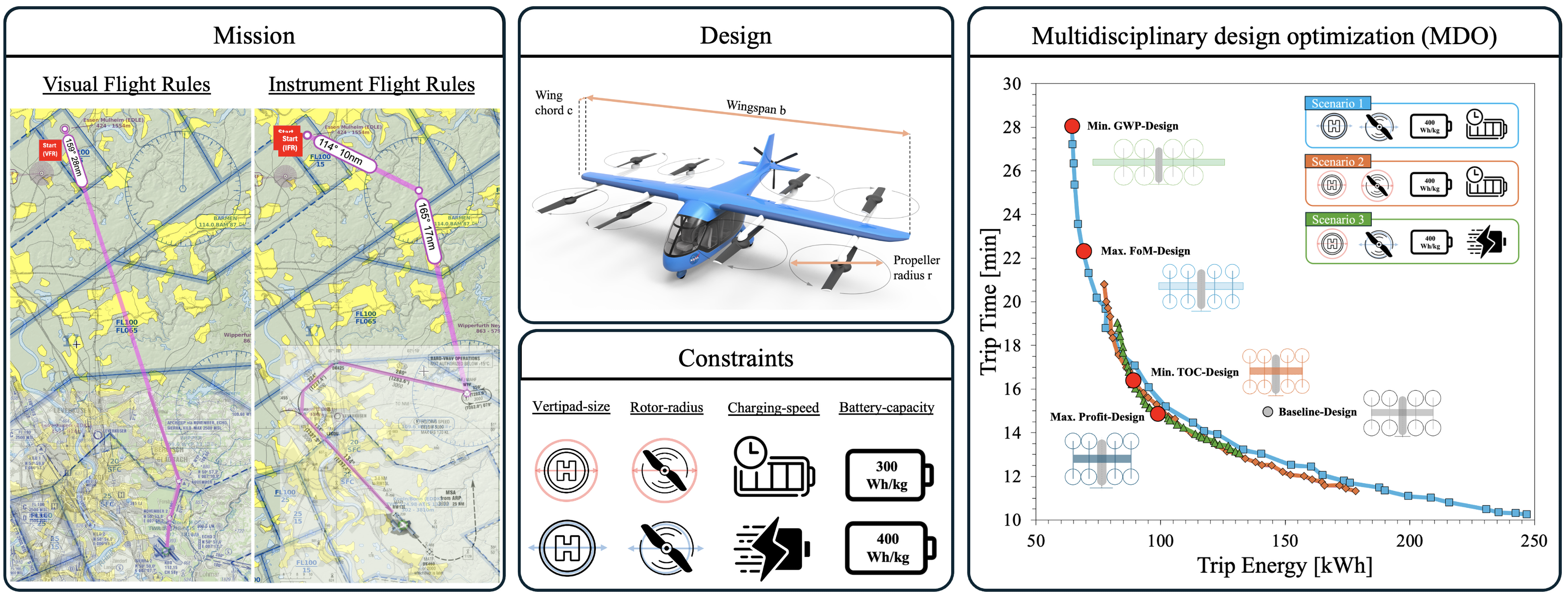
Figure 1: DO of an eVTOL system: mission profiles (visual flight and instrument flight rules VFR and IFR), key design parameters, operational constraints, and trade-off analyses for cruise energy and time. The optimization objectives are the minimization of global warming potential (GWP), total cost of ownership (TOC), maximization of a custom figure of merit, and operational profitability under different eco-system conditions (illustration adapted from [4, 5]).

Developing a comprehensive MDO framework for eVTOLs is crucial for addressing the complex trade-offs in UAM. Existing research mainly optimizes aerodynamic performance, structural properties, and mission efficiency. Table 1 summarizes relevant eVTOL design and mission optimization literature. Several recent studies have achieved reductions in vehicle weight and improvements in energy efficiency, which are both crucial for operational feasibility [6, 7]. Despite extensive MDO research [6, 8, 7, 9, 10], however, critical aspects such as economic viability and environmental impact remain unexplored. Other studies suggest potential enhancements in mission efficiency and cost reduction but also expose significant gaps in addressing operational factors, particularly in sustainability, operations modeling, and vehicle utilization [11, 12]. Areas such as carbon footprint and battery lifecycle are only rarely considered [13, 1]. Clearly, there is a need for a more integrated approach that incorporates profitability and other objectives of potential future eVTOL operators into early-stage design optimization.

Authors	Year	Objective
Kaneko et al. [6]	2023	Optimize eVTOL aerodynamics and energy efficiency for weight reduction.
Sarojini et al. [7]	2023	Optimize lift+cruise [14] weight using a geometry-centric approach.
Ruh et al. [9]	2024	Integrate physics-based models in MDO to optimize design.
Ha et al. [11]	2019	Optimize mission efficiency and profitability in eVTOL designs.
Chinthoju et al. [12]	2024	Cost optimization by varying mass, rotor radius, wing span, cruise speed.
Brown et al. [13]	2018	Design & economic optimization using geometric programming.
Kiesewetter et al. [1]	2023	Holistic UAM ecosystem state of research review & evaluation.
Silva et al. [15]	2018	Examination of lift+cruise vehicle for research & industry guidance.
Patterson et al. [14]	2018	Guideline to study UAM missions & exploration of mission requirements.
Yang et al. [16]	2021	Impact of charging strategies on battery sizing and utilization.
Kasliwal et al. [17]	2019	Physics-based analysis of VTOLs emissions vs. ground-based cars.
Schäfer et al. [2]	2019	Energy, economic and environmental implications of all-electric aircraft.
André et al. [18]	2019	Comprehensive eVTOL life-cycle assessment and design implications.
Mihara et al. [19]	2021	Cost analysis for diverse eVTOL configurations.
Lio et al. [20]	2024	Techno-economic feasibility analysis of eVTOL air taxis.

Table 1: Related eVTOL design and mission optimization literature.

The framework we develop guides the exploration of complex decision-making processes in eVTOL design, aiming to provide valuable insights and recommendations for the development of efficient, sustainable, and economically viable urban air mobility eVTOL systems and operation strategies.

2 Related work

Table 1 summarizes related eVTOL design and mission optimization work. Brown et al. [13] employed geometric programming to optimize vehicle components and mission profiles, including noise calculations and a general cost model. However, the study provided limited detail on cost breakdowns for infrastructure, regulatory compliance, and long-term maintenance. Additionally, it did not fully address environmental costs related to energy production and battery degradation, which are essential for a comprehensive evaluation of the economic and environmental sustainability of UAM. Recent reviews have highlighted significant gaps in integrating economic models for evaluating cost-effectiveness, lifecycle costs, and environmental impacts in eVTOL design [1].

The eVTOL analysis framework developed in [15] and [14] provides insightful guidelines for eVTOL aircraft architecture and mission design that can be adapted to short- and mid-range lift and cruise eVTOL missions. Key insights on battery behavior and its implications for operational charging strategies can be drawn from [16] and [17], and critical perspectives on the interplay between economics, technology, and sustainability in fully electric aircraft are offered in [2], highlighting their interlinked nature, with [18] and [21] providing essential considerations for the environmental impacts of battery usage. A framework for standardized cost model structuring is provided in [22], and valuable input on revenue modeling is provided in [19, 20]. Finally, economic key requirements are defined for real-world operations in [23], useful for validation in eVTOL MDO.

We incorporate ideas from these works into our framework and focus on economic considerations alongside sustainability, aiming to enhance the understanding of trade-offs in aircraft design and contribute to more sustainable and economically viable UAM solutions.

3 Methodology

3.1 Multidisciplinary Design Optimization

Our eVTOL design method uses a GA to solve the multi-objective, multidisciplinary design optimization. Compared to gradient-based methods, GAs can effectively handle complex, multimodal, and non-smooth objective functions with multiple objectives and discrete design variables [8]. GAs iteratively evolve a population of design solutions through selection, crossover, and mutation, allowing for the simultaneous optimization of multiple conflicting objectives [8]. By maintaining a diverse population and utilizing fitness-based selection, the algorithm identifies a set of non-dominated solutions, which collectively form the Pareto front, representing the optimal trade-offs between the objectives. Table 2 summarizes the optimization problem statement. Figure 2 illustrates the extended design structure matrix [24] and the followed design approach for simultaneous minimization of trip time and trip energy requirements. The data is further processed to the mass model for design validation, cost model for economic valuation, and FoM model for comparative classification. The models are introduced in the following subsections, and described in detail in the supplementary material.

Figure 2: Extended Design Structure Matrix for single-objective optimization (FoM, blue arrow), and multi-objective design optimization (time and energy, red arrow).

====		Function/Variable	Description
minimize		$E_{\text{trip}}$	Total energy consumption for the trip (Wh)
		$t_{trip}$	Total time needed for the trip (seconds)
by varying	design	$R_{lifter}$	Lifting rotor radius (m)
		$R_{pusher}$	Pusher rotor radius (m)
		$c$	Aircraft wing chord (m)
		$b$	Aircraft wing span (m)
		$MTOM$	Maximum take-off mass (kg)
subject to	design	$1\leq R_{lifter}\leq 1.5|2.0$	Lifting rotor constraint (m)
		$1\leq R_{lifter}\leq 1.5|2.0$	Pusher rotor constraint (m)
		$1\leq c\leq 3$	Chord bounds, based on comparable aircraft [25]
		$\rho_{\text{bat}}\leq 400$	Battery energy density (Wh/kg) [1]
		$MTOM\leq 5.700kg$	Maximum takeoff mass constraint [26]
		$b_{min}\geq 2\cdot(3\cdot R_{prop_{hover}}+2\cdot d+\frac{w}{2})$	wing constraint (m)
		$15\geq 2\cdot(2\cdot d+4\cdot R_{prop_{hover}}+\frac{w}{2})$	Vertiport constraint (m) [27]
		$MTOM\cdot 1.02=m_{empty}+m_{bat}+m_{pay}$	Mass budget (kg), allowed for 2% deviation
	profile	$V\leq 129$	Low airspace velocity bound (m/s) [28]

Table 2: eVTOL multidisciplinary design optimization.

3.1.1 Mass Estimation

The maximum take-off mass ($MTOM$) consists of the payload mass $M_{payload}$, the eVTOL empty mass $M_{empty}$, and the battery mass $M_{battery}$:

$$MTOM=M_{payload}+M_{empty}+M_{battery}\leq Limit_{certification}.$$ (1)

According to the European Union Aviation Safety Agency’s (EASA) latest certification specifications for eVTOL, the maximum certifiable mass is limited to $Limit_{certification}=5{,}700\,\text{kg}$ [29]. $M_{battery}$ is considered separately from $M_{empty}$ due to the significant impact the batteries have on the MTOM, and as batteries can be exchanged flexibly if necessary. $M_{battery}$ is calculated using the following equation taking into account the design mission energy requirements and battery energy density $\rho_{bat}$ in Wh/kg, with a factor of 0.64 to account for unusable battery energy (introduced in section 3.1.3):

$$M_{battery}=\frac{E_{useable}}{e_{usable}}=\frac{E_{trip}+E_{res}}{0.64\cdot\rho_{bat}}.$$ (2)

The empty mass ($M_{empty}$) is defined as:

$$M_{empty}=M_{wing}+M_{rotor}+M_{motor}+M_{fuselage}+M_{systems}+M_{furnish}+M_{crew},$$ (3)

where $M_{wing}$, $M_{fuselage}$, $M_{systems}$, and $M_{furnish}$ are estimated according to Raymer [30] and Nicolai [31], relying on data from general aviation aircraft. $M_{furnish}$ is the predicted weight of furnishings, non-structural components that are necessary to equip the aircraft for the operation and comfort of the crew and passengers. Crew mass $M_{crew}$ is based on average masses for single pilot operation [32]. The model for $M_{rotor}$ is based on [6], and $M_{motor}$ is based on [33]. $M_{payload}$ accounts for average mass of passenger $M_{pax}$ and luggage per passenger $M_{lug}$ [32], calculated as:

$$M_{payload}=(M_{pax}+M_{lug})\cdot n_{seats}\cdot LF.$$ (4)

Here, we consider a fully loaded 4-seater eVTOL (excl. pilot) as sizing requirement, resulting in a fixed payload of:

$$M_{payload}=(82.2+16)\cdot 4=392.8kg$$ (5)

3.1.2 Aerodynamic Model

We use a simplified aerodynamic lift and drag coefficient model of the eVTOL wing [6, 34], and use airfoil data for a NACA2412 airfoil at $Re=200,000$ [35]. While this simplified model is convenient for fast optimization and allows for the consideration of multiple subsystems, the same framework can be extended to more complex models in future work. The model for the lift coefficent $C_{L}$ assumes a linear pre-stall lift curve, using the finite-wing lift coefficient:

$$C_{L}=\frac{\alpha_{airfoil}}{1+\frac{\alpha_{airfoil}}{\pi\cdot AR\cdot e}}\cdot\alpha+C_{L_{0}},$$ (6)

where $\alpha_{airfoil}$ is the airfoil lift-curve slope, $AR$ is the wing aspect ratio, and $e$ is the Oswald efficiency factor. Total lift is then calculated as:

$$L=\frac{1}{2}\cdot\rho\cdot V^{2}\cdot S\cdot C_{L}=\frac{1}{2}\cdot\rho\cdot V^{2}\cdot S\cdot\left(\frac{\alpha_{airfoil}}{1+\frac{\alpha_{airfoil}}{\pi\cdot AR\cdot e}}\cdot\alpha+C_{L_{0}}\right).$$ (7)

The model for the drag coefficient $C_{D}$ is based on lifting line theory [34], and assumes that the finite-wing drag coefficient is composed of induced drag $C_{D_{i}}$ and parasite drag $C_{D_{min}}=0.0397$ [6]:

$$C_{D}=C_{D_{min}}+C_{D_{i}}=C_{D_{min}}+\frac{C_{L}^{2}}{\pi\cdot AR\cdot e}.$$ (8)

The total drag is then calculated as:

$$D=\frac{1}{2}\cdot\rho\cdot V^{2}\cdot S\cdot C_{D}=\frac{1}{2}\cdot\rho\cdot V^{2}\cdot S\cdot\left(0.0397+\frac{C_{L}^{2}}{\pi\cdot AR\cdot e}\right).$$ (9)

3.1.3 Power & Energy Model

The power requirements for hover $P_{hover}$, climb $P_{climb}$, and cruise $P_{cruise}$ are computed using momentum theory, based on thrust requirements of the respective flight phase $T_{req}$, rotor diameter $R$, max. take-off mass, air density $\rho$, induced velocity $v_{i}$, climb angle $\theta$ (assuming zero wind, thus $\theta=\alpha$) and propulsion efficiency $\eta$:

$$P_{hover}=\frac{MTOM\cdot g}{\eta_{h}}\cdot\sqrt{\frac{\sigma}{2\cdot\rho}}=\frac{MTOM\cdot g}{\eta_{h}}\cdot\sqrt{\frac{T_{prop}}{2\cdot\rho\cdot\pi\cdot R_{prop}^{2}}},$$ (10)

$$P_{climb}=P_{req_{flight}}+P_{ind_{prop}}=\frac{T_{req_{climb}}\cdot V_{climb}}{\eta_{c}}+\frac{T_{prop_{climb}}\cdot v_{i}}{\eta_{c}}\cdot n_{prop},$$ (11)

$$P_{cruise}=P_{req_{flight}}+P_{ind_{prop}}=\frac{T_{req_{cruise}}\cdot V_{cruise}}{\eta_{c}}+\frac{T_{prop_{cruise}}\cdot v_{i}}{\eta_{c}}\cdot n_{prop}.$$ (12)

The time requirement for each flight phase is calculated considering the speeds for climb $V_{climb}$ and cruise $V_{cruise}$:

$$V_{climb}=\sqrt{\frac{2\cdot MTOM\cdot g\cdot cos(\theta)}{\rho\cdot S\cdot C_{L_{climb}}}},$$ (13)

$$V_{cruise}=\sqrt{\frac{2\cdot MTOM\cdot g}{\rho\cdot S\cdot C_{L_{cruise}}}},$$ (14)

whereby hover time is assumed to be fixed at a total of 60 seconds [23]. This results in the distance-bridging energy requirement for the sizing mission:

$$E_{trip}=\sum_{i}P_{i}\cdot t_{i}=P_{hover}\cdot t_{hover}+P_{climb}\cdot t_{climb}+P_{cruise}\cdot t_{cruise}.$$ (15)

The maximum usable trip energy in the battery results from the consideration of 30min reserve in cruise power conditions, and unusable energy in the battery. The unusable energy is derived from 10% ceiling and 10% floor state-of-charge (SOC), and the assumption that the battery is operated in its end-of-life (EOL) state, defined by a 20% degradation [16], resulting in specific battery energy at EOL:

$$e_{BAT_{EOL}}=0.8\cdot\rho_{bat}.$$ (16)

For a given battery energy density $\rho_{bat}$ in Wh/kg, the usable specific energy available for the sizing mission is:

$$e_{\text{usable}}=0.8\cdot e_{BAT_{EOL}}=0.64\cdot\rho_{bat}=e_{trip_{sizing}}+e_{reserve}.$$ (17)

3.1.4 Economic Model

The economic model consists of a cost model based on Air Transport Association (ATA) [22] and a revenue model inspired by UberElevate [23, 36]. The operations are based on Uber’s assumptions of 280 annual working days per eVTOL with an 8-hour operating window. Real-world operation windows need to be evaluated more closely in light of regional weather conditions and weather statistics, as it can be assumed that eVTOLs will initially operate exclusively under visual flight rules, which excludes operations in hazy weather [1]. Total operating costs per flight (TOC) are defined as the sum of cash operating costs (COC), cost of ownership (COO) and indirect operating costs (IOC). The sum of COC and COO is defined as direct operating costs (DOC):

$$TOC=COC+COO+IOC,$$ (18)

with IOC being a fixed percentage of 22% of DOC [37]. COC are directly related to flight operations taking into account energy costs $C_{E}$, crew costs $C_{C}$, navigation/ATC costs $C_{N}$ and maintenance costs $C_{M}$. $C_{M}$ is the sum of wrap-rated maintenance costs $C_{wrm}$ according to [13] and battery replacement costs $C_{MB}$:

$$COC=C_{E}+C_{C}+C_{N}+C_{wrm}+C_{MB}.$$ (19)

COO accounts for insurance $C_{ins}$, as 6% of COC [19], and capital expenditure, as annual depreciation costs $C_{dep}$ [38]:

$$COO=C_{ins}+C_{dep}.$$ (20)

The profit model is based on the revenue calculation using a fixed kilometer-based fee [23]. This fee is based on the mileage rate for trips during the day of London cabs [39] as a first estimation:

$$Profit_{\text{flight}}=Rev-TOC=fare\cdot d_{\text{trip}}-TOC.$$ (21)

3.1.5 Global Warming Potential Model

The global warming potential (GWP) considered in this work is derived from the GWP impact of electricity generation and the life-cycle emissions of the batteries used. The GWP impact of the energy consumed is based on the International Energy Agency (IEA) data for Germany [40, 41, 42], assumed as 0.38 kg $CO_{2}$-eq per kWh. However, our framework also allows for the application of the energy production GWP of a large number of other regions. A simple empirical battery degradation model is, which is detailed in appendix B.5. We model the life-cycle of a lithium-ion battery based on the depth of discharge, battery charging rate, and flight phase average battery discharge rate. If we relate the life-cycle of the battery to the operational charging cycles, we can calculate the number of batteries required annually. According to [21], we assume a life-cycle GWP of 124.5 kg $CO_{2}$-eq per kWh battery capacity, based on Nickel-Cobalt-Manganese (NCM) lithium-ion batteries, which are widely used in electric vehicles (EVs) and increasingly in aviation due to their high energy density and favorable weight-to-performance ratio [1]. The GWP of this battery accounts for raw material extraction and processing, battery manufacturing, transportation, and end-of-life treatment [18]. Note that the GWP-impact calculation in this framework does not take the eVTOL life-cycle into account. Nonetheless, the presented framework and analysis can be expanded to include this aspect in future work, e.g. based on the work in [18].

3.1.6 eVTOL Transportation Figure of Merit

The transportation Figure of Merit (FoM) for an eVTOL is computed by comparing its performance to various transportation modes in terms of time, CO₂-eq emissions, and cost per seat-kilometer. The FoM is calculated using the following equation:

$$FOM=w_{t}\cdot R_{t}+w_{CO2e}\cdot R_{CO2e}+w_{cost}\cdot R_{cost},$$ (22)

where $R_{t}$, $R_{CO2}$, and $R_{cost}$ are the normalized ratings for time, CO₂, energy, and cost, respectively, and $w_{t}$, $w_{CO2}$, $w_{energy}$, and $w_{cost}$ are the corresponding weights assumed equally distributed. The rating for each criterion is computed using the following formula:

$$\text{Rating}=\frac{(x-X_{\text{min}})-10\cdot(x-X_{\text{max}})}{X_{\text{max}}-X_{\text{min}}},$$ (23)

where $x$ is the value being rated, $X_{\text{min}}$ is the minimum value, and $X_{\text{max}}$ is the maximum value within each criterion. The eVTOL is compared to battery electric vehicles (BEV), gasoline & diesel internal combustion engine vehicles (GICEV, DICEV), public buses, trains, bicycles, and airplanes for various load factors.

3.2 Analysis Workflow

The methodology is centered around the MDO framework, using a GA solver to explore and evaluate various design scenarios. The workflow initiates with the definition of macro scenarios, which outline broad conditions under which the designs will be evaluated. Simultaneously, specific constraint scenarios are set to impose necessary limitations on the design space. These scenarios are essential to ensure that the optimization process considers all relevant factors, including operational, economic, and sustainability constraints. Those scenarios are described in detail in section 3.4.

We perform an MDO for each scenario, generating a Pareto front that represents a set of non-dominated design solutions. This Pareto front provides the foundation for the decision-making process, where each objective is evaluated across the design space. For each objective — minimizing Global Warming Potential, minimizing total operating cost, maximizing profit, and optimizing the transportation Figure of Merit — the specific behavior of the objective across the design space is analyzed. For instance, to identify the design that minimizes TOC, the curve representing TOC as a function of the design space is overlaid on the Pareto front. This allows for the selection of the design that achieves the minimum TOC within the feasible region defined by the Pareto front. Similar decision-making processes are applied to identify the designs that optimize other objectives. These trade-off designs, representing optimal solutions for each objective, are discussed in chapter 4.7. This process ensures that each selected design is not only Pareto-optimal but also specifically tailored to achieve the desired objective within the broader design space. After generating and analyzing the Pareto front, a baseline scenario is established to serve as a reference point. A comparative analysis is then conducted to evaluate the performance of each design across the different scenarios. The impact of constraints is also analyzed to understand how they influence the trade-off balance between design, sustainability, operations, and economics. This structured approach allows for a comprehensive exploration of eVTOL designs, ensuring that the final selection is well-balanced across multiple criteria and optimized for real-world application.

3.3 Sizing Mission

This study adopts the sizing mission profile proposed by National Aeronautics and Space Administration (NASA) [14], which is characterized by a 37.5 nautical mile ($\sim$70 km) travel distance and a cruise altitude of 4.000ft above ground level (AGL), shown in Figure 3. This widely accepted mission profile aligns with established research ([15], [14]), enhancing the comparability of the presented findings within academic and industry contexts.

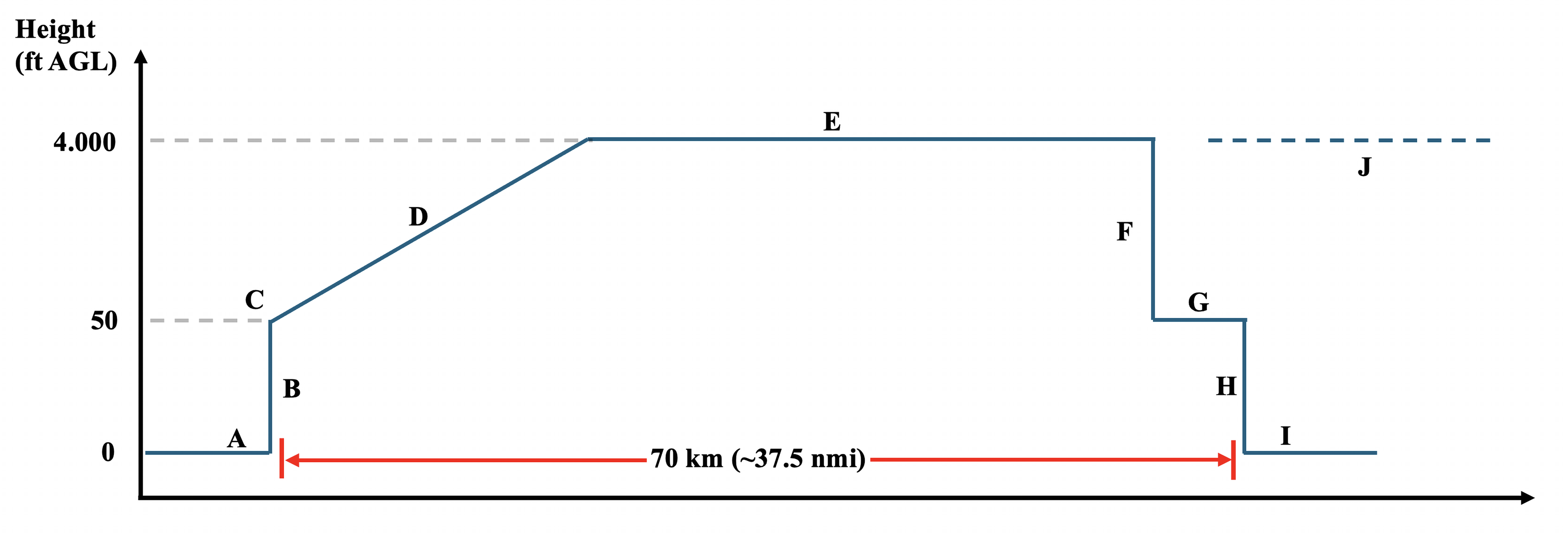
(a) Sizing mission profile.

Segment	Description
A	Take-off
B	Vertical climb to 50ft (30s hover)
C	Transition
D	Climb
E	Cruise at 4,000ft
F	No credit descent
G	Transition
H	Vertical descent from 50ft (30s hover)
I	Landing
J	30 min reserve

(b) Sizing mission segments.

Figure 3: Sizing mission: (a) profile and (b) segments.

The use of these parameters reflects realistic operational conditions for urban and regional air mobility, including typical city-to-city or intra-urban flights. By incorporating key operational phases such as vertical climb, cruise climb and cruise, this mission profile provides comprehensive insights into eVTOL performance, including energy consumption and battery requirements. Additionally, a 30-minute reserve is maintained in accordance with EASA and Federal Aviation Administration (FAA) Visual Flight Rules (VFR) requirements. According to [43], eVTOLs face severe range limitations under Instrument Flight Rules (IFR) conditions due to strict reserve requirements of 45min cruise and current battery constraints, making them impractical for most missions outside ideal weather. Significant battery improvements are needed before eVTOLs can reliably operate in diverse environments. This standardized approach ensures methodological rigor and facilitates future research by providing a coherent framework for further studies.

3.4 Design Scenario Classification

The scenarios defined in Table 3 serve as inputs for the proposed MDO framework. These scenarios display the macro and constraint conditions under which the optimization is performed. By systematically exploring the "Open" and "Restricted" scenarios across various parameters such as charging infrastructure, propeller radius, vertiport dimensions, and battery energy density, the analysis effectively evaluates and compares the performance of different eVTOL designs. This structured scenario approach enables a comprehensive assessment of the design space, facilitating informed decision-making based on varying operational and technological constraints, described in Appendix B.6. This approach allows for a targeted investigation into how different scenarios influence eVTOL designs, providing critical insights into the specific requirements and constraints necessary for optimizing eVTOL configurations. Through this analysis, we can identify key trade-offs and design considerations that are essential for aligning the technical capabilities of eVTOLs with the anticipated operational environments.

Scenario	Open	Restricted
Charging	4C: Supports rapid charging enabling faster service cycles as intended by various UAM providers [1].	1C: Assumes slow charging, offering a conservative scenario, especially in urban areas with limited fast-charging.
Prop-Radius	A 2m propeller radius allows exploration of scenarios with fewer spatial and noise constraints, suitable for suburban or rural eVTOL applications.	The 1.5m propeller radius aligns with industry benchmarks and UAM constraints, offering a realistic framework for current designs (see supplementary material in Chapter 6 for industry comparison).
Vertiport	Not limiting vertiport dimensions allows exploration of larger, more flexible designs, supporting future infrastructure in less constrained environments.	15m circular dimension reflects urban space limitations and integration challenges with existing urban infrastructure [44].
Battery $\rho_{bat}$	The 400 Wh/kg assumption anticipates future battery advancements, aligning with industry targets and enabling extended range and performance scenarios [1].	The 300 Wh/kg assumption represents the current state of lithium-ion technology, providing a conservative and realistic baseline for today’s eVTOL designs.

Table 3: Case definition: open vs restricted scenarios for eVTOL operations.

4 Results

We explore four scenarios with different eVTOL design-objectives, illustrated in Table 4. We analyze the trade-offs involved in the specialized eVTOL designs and discuss the regulatory and operational framework requirements implied by each design. For each of the existing constraint scenarios in Table 4, we analyze an eVTOL design space for the objectives (1) maximum annual profit, (2) minimum operating cost per trip, (3) minimum annual GWP, and (4) maximum FoM. The constraint scenarios in which the respective objectives are achieved are marked with the corresponding entry in Table 4.

	Slow-charging Prop-open	Slow-charging Prop-restricted	Fast-charging Prop-open	Fast-charging Prop-restricted
Vertiport-open $\rho_{Battery}=$$300Wh/kg$
Vertiport-open $\rho_{Battery}=$$400Wh/kg$	Min. GWP- and Max. FoM scenario
Vertiport-restricted $\rho_{Battery}=$$300Wh/kg$				Baseline scenario
Vertiport-restricted $\rho_{Battery}=$$400Wh/kg$		Min. TOC scenario	Max. profit scenario

Table 4: Matrix of design scenario results.

4.1 Baseline Specification

The baseline scenario in Table 4 aligns with the assumptions of UAM such as the operational adaptability of existing heliports, the accessible 300 Wh / kg battery density, and fast charging [16]. The design focuses on maximizing annual profit and serves as a benchmark, illustrated in Figure 4 and compared to NASA’s lift+cruise vehicle [15] and industry insights [1] (see industry design comparison in supplementary material in Chapter 6). The main difference between the baseline and NASA designs is the balance between practical industrial and academic optimization. The baseline design relies on conservative battery density and moderate aerodynamic design for technical feasibility, while the NASA design maximizes efficiency with higher aspect ratio and increased battery density, but implies structural and operational challenges due to higher empty mass and reduced cruise speed.

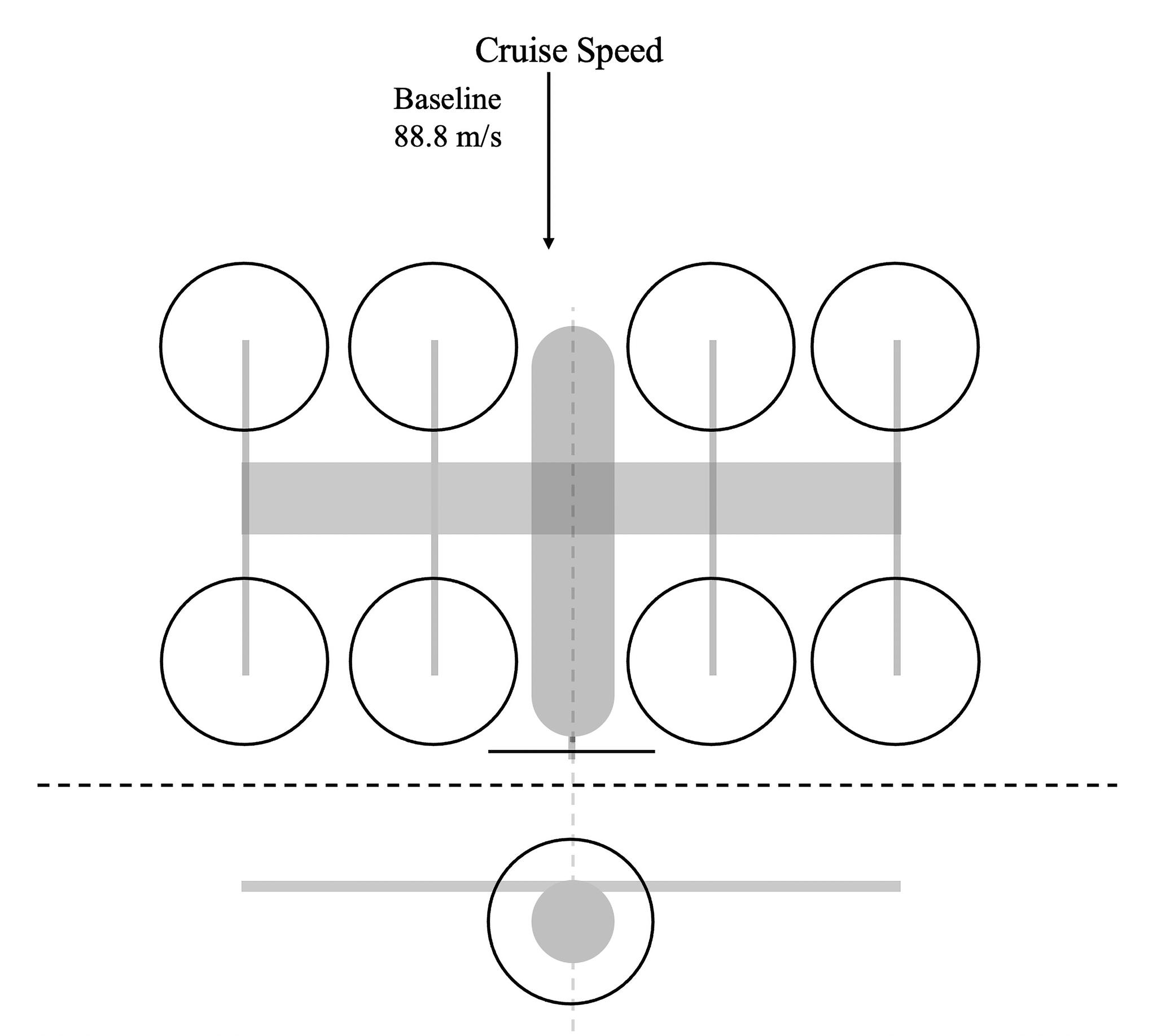
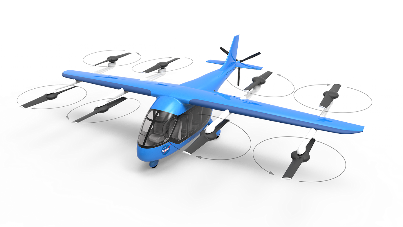
Description (Units)	Baseline	NASA [15]	%-$\Delta$
MTOM (kg)	3.660	3.724	-1.72
Empty Mass (kg)	1.434,32	2.725,10	-47.37
Payload (kg)	392	544	-27.90
Wing Span (m)	12.85	13.8	-6.88
Lifter Radius (m)	1.47	1.50	-1.74
Aspect Ratio	9.88	12,70	-22.18
Wing Loading (kg/m2)	218.97	248.27	-11.80
Disk Loading (kg/m2)	67.04	65.85	-1.80
Battery Density (Wh/kg)	300	519.40	-42.24
Battery Capacity (kWh)	605.01	398.88	51.68
Cruise Speed (km/h)	320.40	169.8	88.69
Hover C-rate	1.45	1.90	-18.77
Cruise C-rate	0.81	0,6	34.40
Charging C-rate	4.0	N/A	-

Figure 4: Left: baseline configuration (illustration adapted from [4]). Right: table with aircraft design metrics comparison between baseline and NASA reference eVTOL with relative differences.

4.2 Results and Discussion of the Profit-maximizing eVTOL Design

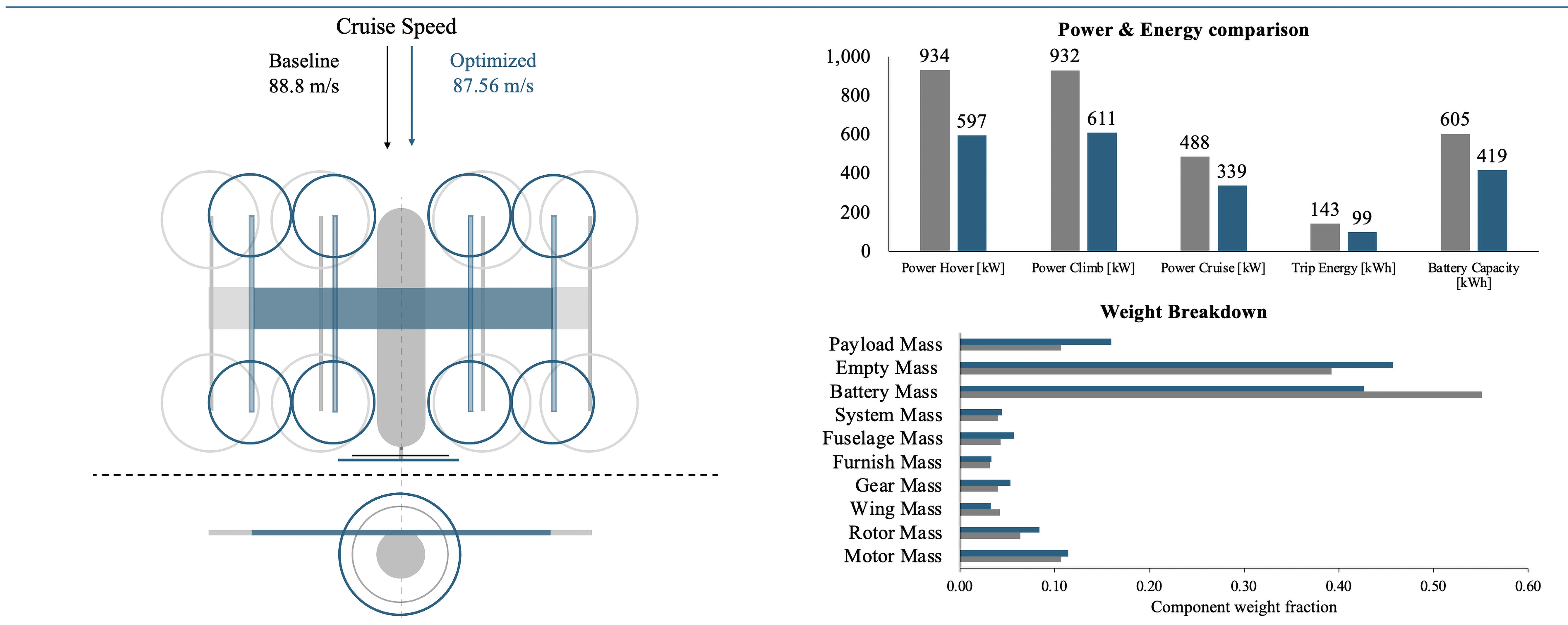
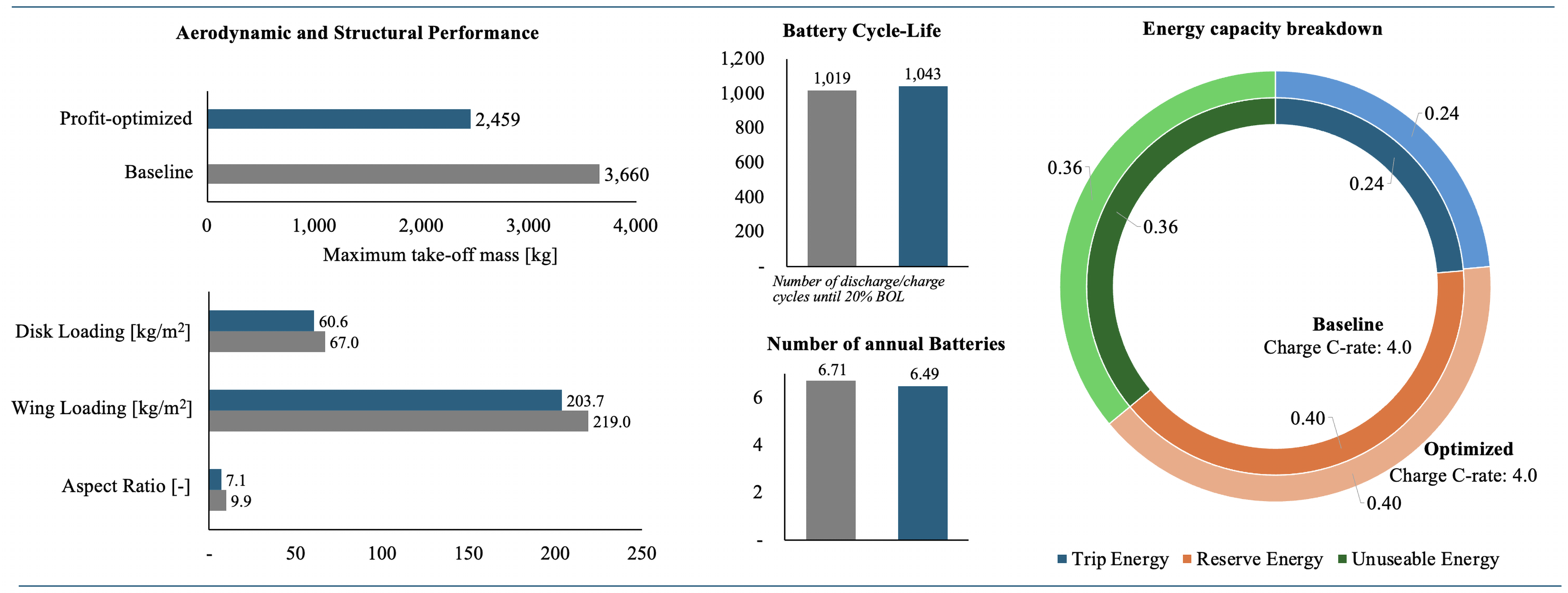
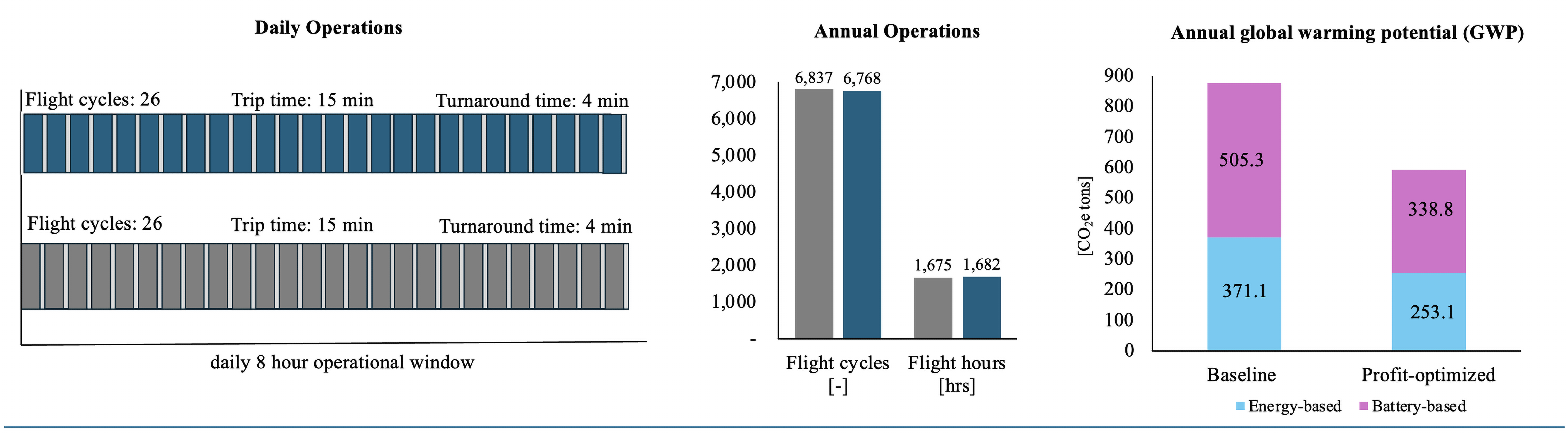
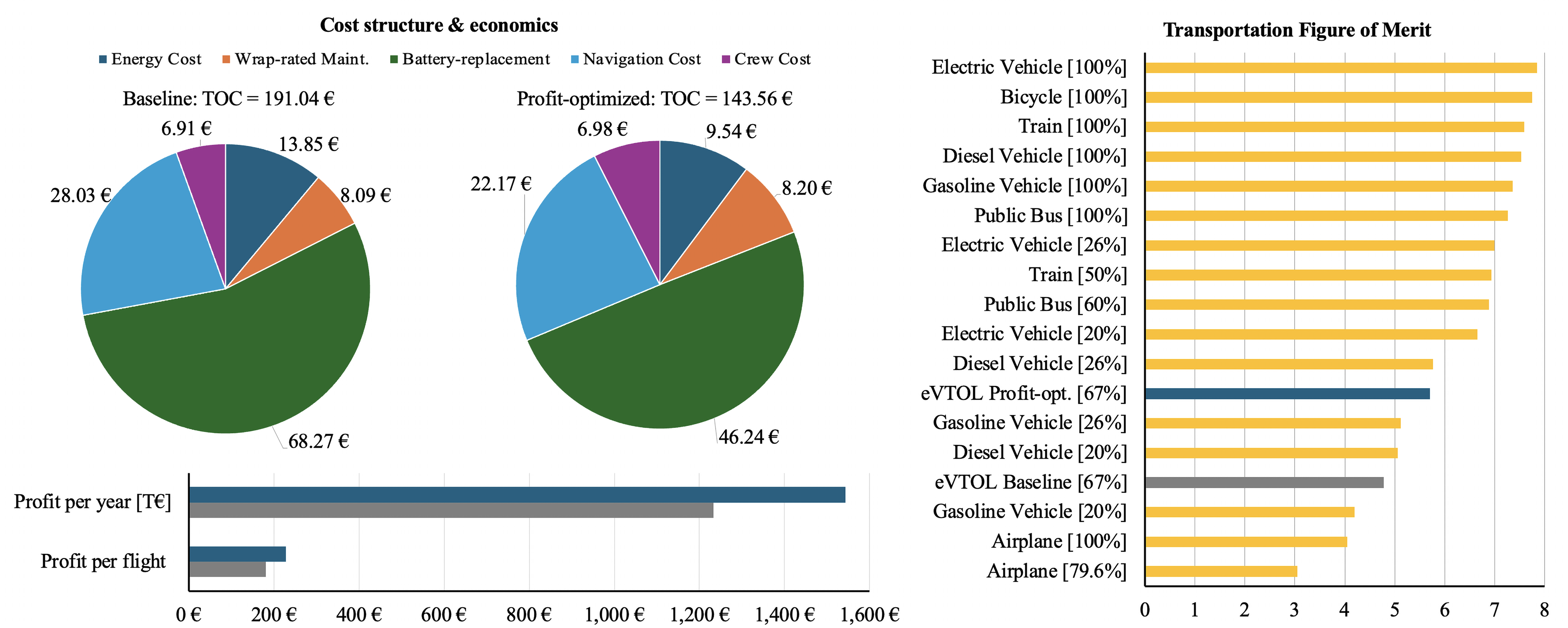
Figure 5: Comparative results of profit-optimized eVTOL design.

The profit-maximizing eVTOL design, shown in Figure 5, is developed within a scenario characterized by the use of fast charging infrastructure (4C), open limits on rotor diameter, and a high battery energy density of 400 Wh/kg. The vertiport dimension is capped at a 15m D-value, making large wingspans less relevant to this design. This scenario prioritizes the maximization of annual profit while maintaining operational efficiency. Figure 12(a) illustrates the relationship between trip time, annual profit, and trip energy on the Pareto front. The analysis shows that increasing trip energy initially leads to higher profits, but beyond an optimal point (around 98 kWh), profits begin to decline. This decline is due to increased TOC (see Figure 12(b)), driven by a rise in energy requirements as a result of high cruise speeds and increasing battery mass. Additionally, the radius of pusher and lifter rotors are slightly smaller to further reduce empty mass by reducing rotor mass, contributing to optimizing hover and cruise efficiency. The 10% reduction in disk loading indicates a trade-off in mass minimization and propulsion design optimization to improve profit margins. The design achieves profit maximization by reducing MTOM by 33%, primarily through improvements in battery storage efficiency. Battery mass is reduced by 48% and empty mass by 32%, which is largely due to a 28% reduction in wing span, lowering structural mass. These mass reductions contribute to a 26% increase in annual profit, driven by a 25% reduction in TOC. This is accomplished while maintaining the same number of flight cycles and flight hours per year, thanks to the fast-charging infrastructure that supports very low turnaround times of just 3 minutes. Consequently, trip times are maintained at 15 minutes with nearly the same average cruise speeds as the baseline. The reduction in TOC is multifaceted: energy costs decrease by 31% due to improved efficiency from the reduced MTOM, battery replacement costs are reduced by 32% as 400 Wh/kg battery density allows for a 32% reduction in battery capacity, lowering battery unit cost by 31%. Navigation costs drop by 21% due to the lower MTOM, and crew costs remain nearly unchanged as they are trip time-based. The reduction in cost of ownership by 25% is mainly due to a 22% decrease in aircraft acquisition costs, which are directly linked to the reduction in empty mass. Moreover, this profit-maximized design achieves a remarkable 32% reduction in annual GWP. The reduction in GWP is primarily due to a 30% decrease in trip energy demands and battery capacity requirements. In the following section on GWP-optimized design, we will see that the environmental impact can be further reduced and therefore environmental impact associated with battery production, particularly the use of materials such as lithium, cobalt, and nickel, remains problematic. These materials are associated with significant environmental and ethical concerns during extraction and disposal, suggesting that further advancements in battery technology are necessary to better align profitability with environmental sustainability. In summary, the design effectively maximizes profit by reducing TOC through strategic weight and efficiency improvements, while maintaining high operational efficiency. However, the environmental trade-offs show that while the design is economically robust, it may need further refinement to achieve its full potential from an environmental feasibility perspective.

4.3 Results and Discussion of the Cost-minimizing eVTOL Design

The TOC-minimizing design, shown in Figure 6, is characterized by several strategic adaptations aimed to reduce total operating costs. Key features of the relevant scenario include a limit in propeller radius and a slow charging infrastructure (1C). The design is also constrained by a vertiport dimension capped at 15 meters, which encourages a low wingspan to further reduce mass. The battery density is set at 400 Wh/kg, ensuring efficient energy storage. Figure 12(b) illustrates the relationship between trip energy and TOC on the Pareto front. The analysis shows that as trip energy increases, TOC rises sharply, indicating that optimizing energy consumption is crucial for cost reduction. The diagram also shows a non-linear relationship between travel energy, travel time, and operating costs; contrary to intuition, minimizing energy is not a cost-minimizing strategy, see Figure 12(b). Energy efficient designs are mainly achieved using high AR wings, leading to diminishing cost advantage related to structural complexity. Minimized costs are found for a balanced energy requirement range, where moderate wing design allows a balance of structure and operational efficiency. This highlights the necessity of balancing energy use and TOC to achieve both efficiency and cost-effectiveness. The TOC-minimizing design reduces TOC by -42% from €191 at baseline to €109.9 per trip, primarily by cutting cash operating costs by 54% and cost of ownership COO by 42%. The most substantial cost saving is an 89% reduction in battery replacement costs, achieved by extending the battery cycle life from 1,019 to 5,667 cycles. This is facilitated by a reduction in battery charging rates, which also reduces battery capacity by 41%, reflecting a more efficient storage system and linearly reduced battery unit costs. Navigation costs, although reduced by 21%, arise as the highest cost element at €20.7 per trip, with time-dependent costs slightly increasing due to extended operational times. The design adapts to achieve these reductions by decreasing cruise speed by 11% to 79 m/s, balancing energy efficiency with operational needs. This adjustment results in a 42% reduction in daily flight cycles, from 26 to 16, due to the increased turnaround time of 15 minutes. Although travel time only increases by one minute compared to the baseline (16 minutes), the reduced number of flight cycles limits annual profit potential. The implementation of battery swapping is proposed as it could mitigate the impact of extended turnaround times and allow this design to pass as profit maximizing, as it already generates a maximum profit per flight of 45% compared to baseline. However, the annual profit is limited due to operational constraints caused by the longer, gentle charging time. Finally, this design also offers significant sustainability benefits, reducing GWP by 81% annually due to improved battery usage and energy efficiency. While TOC minimization is effective, the trade-offs in operations and profitability underscore the importance of further optimization with a focus to enhance viability in real-world applications.

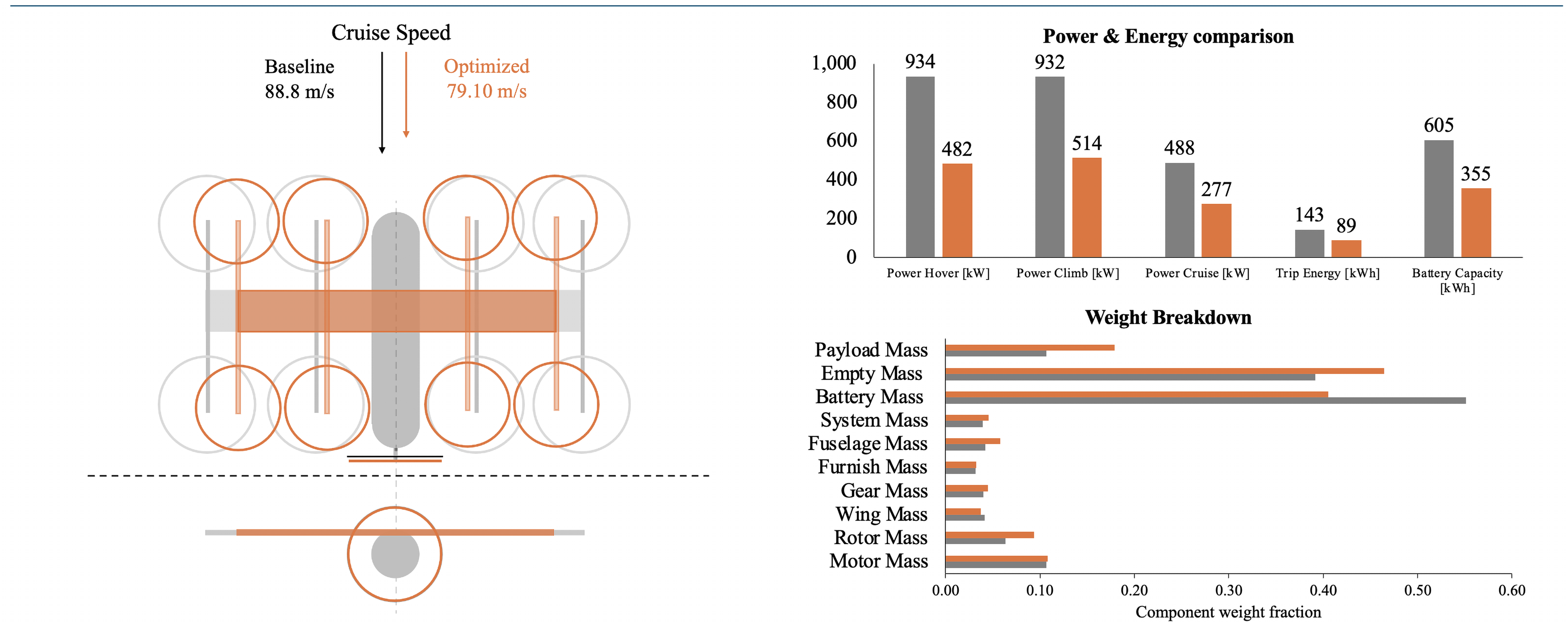
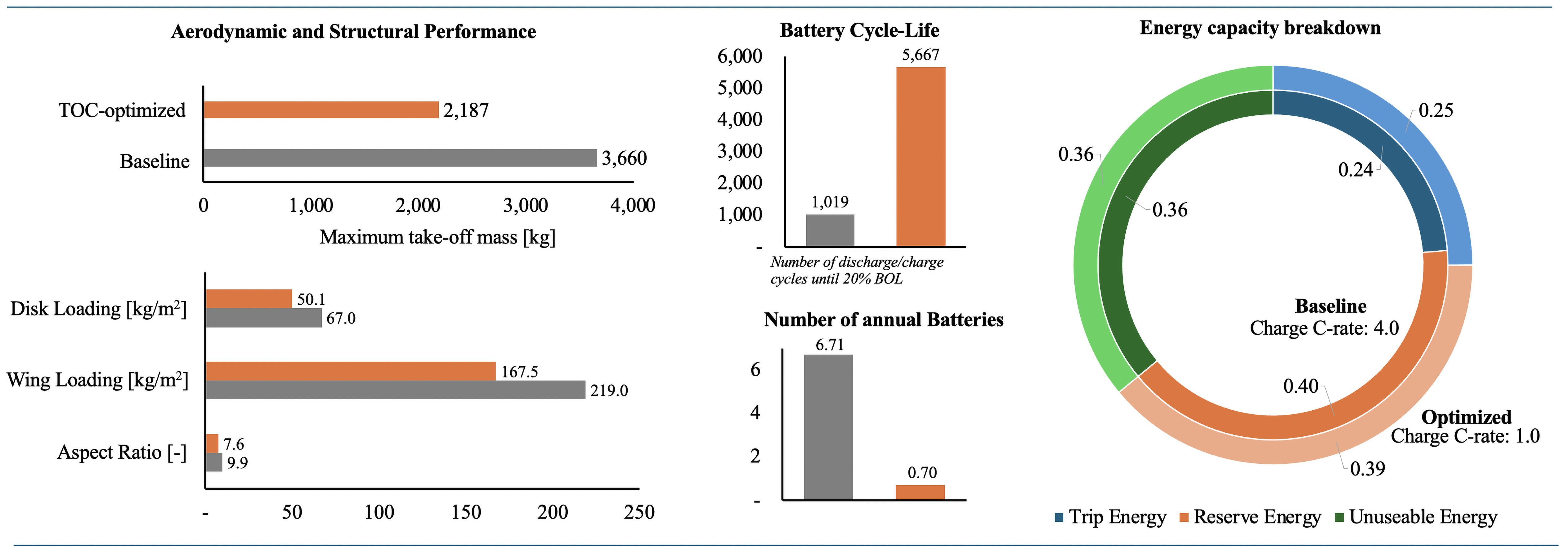
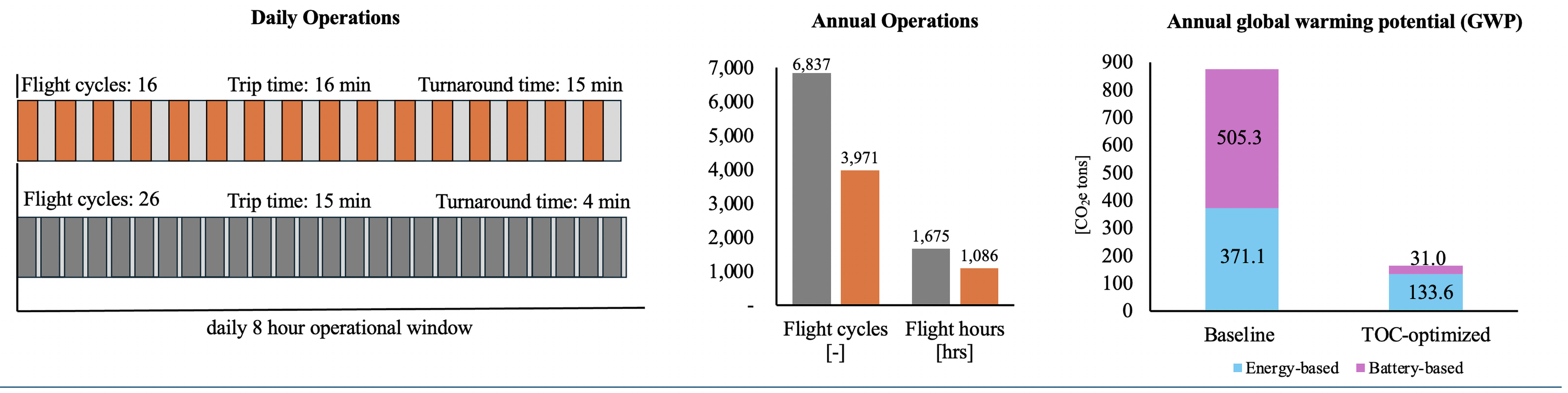
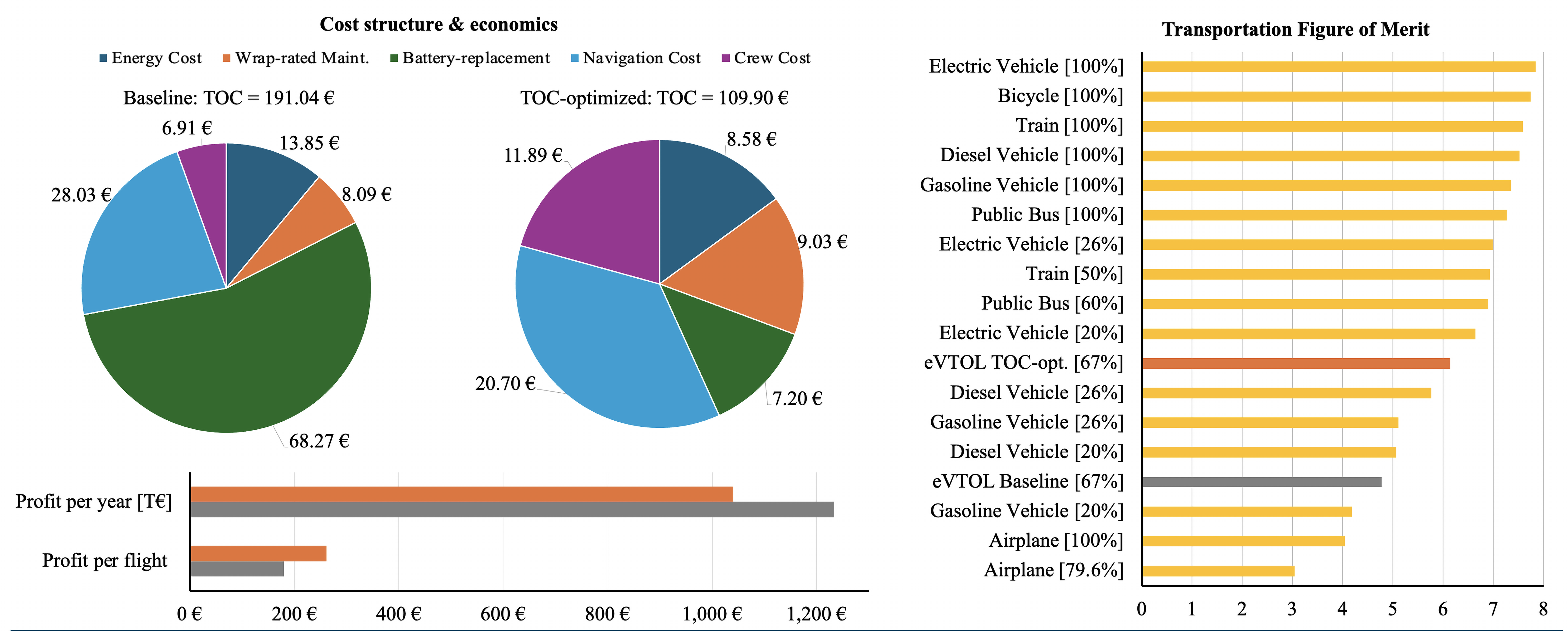
Figure 6: Comparative results of TOC-optimized eVTOL design.

4.4 Results and Discussion of the GWP-minimizing eVTOL Design

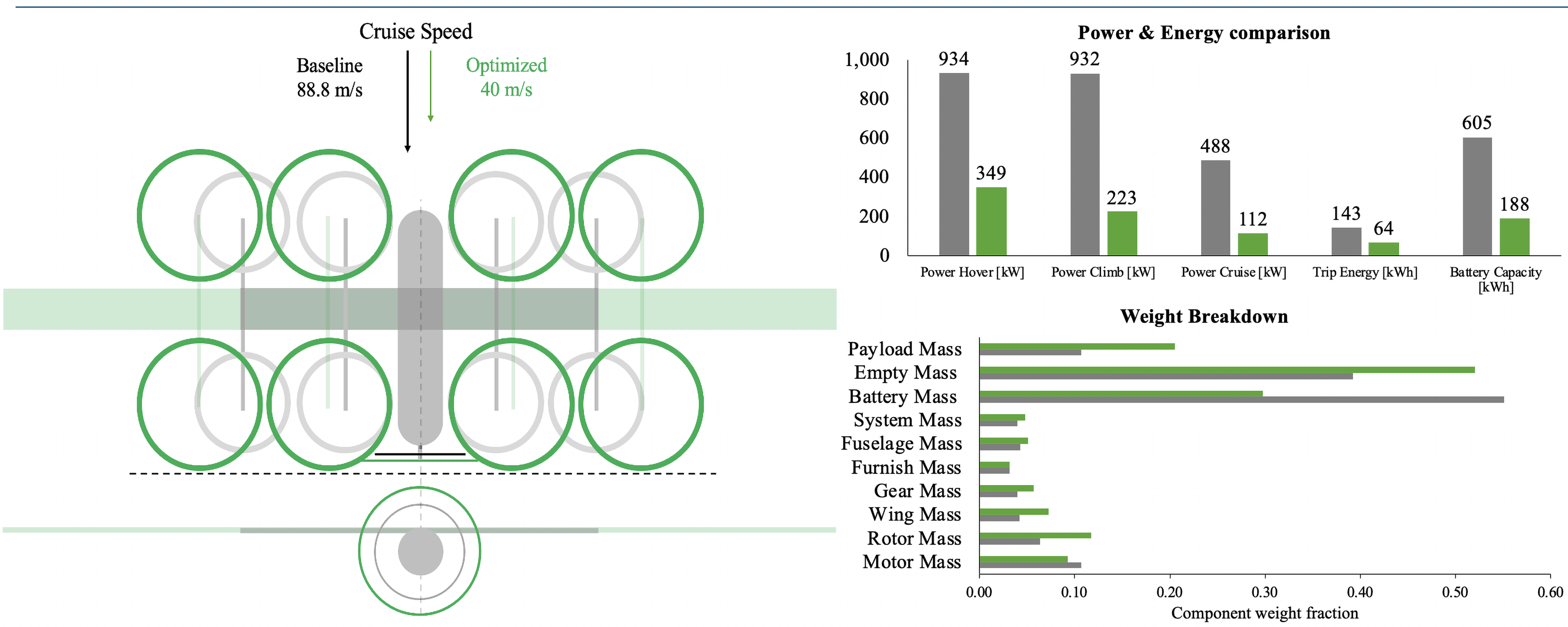
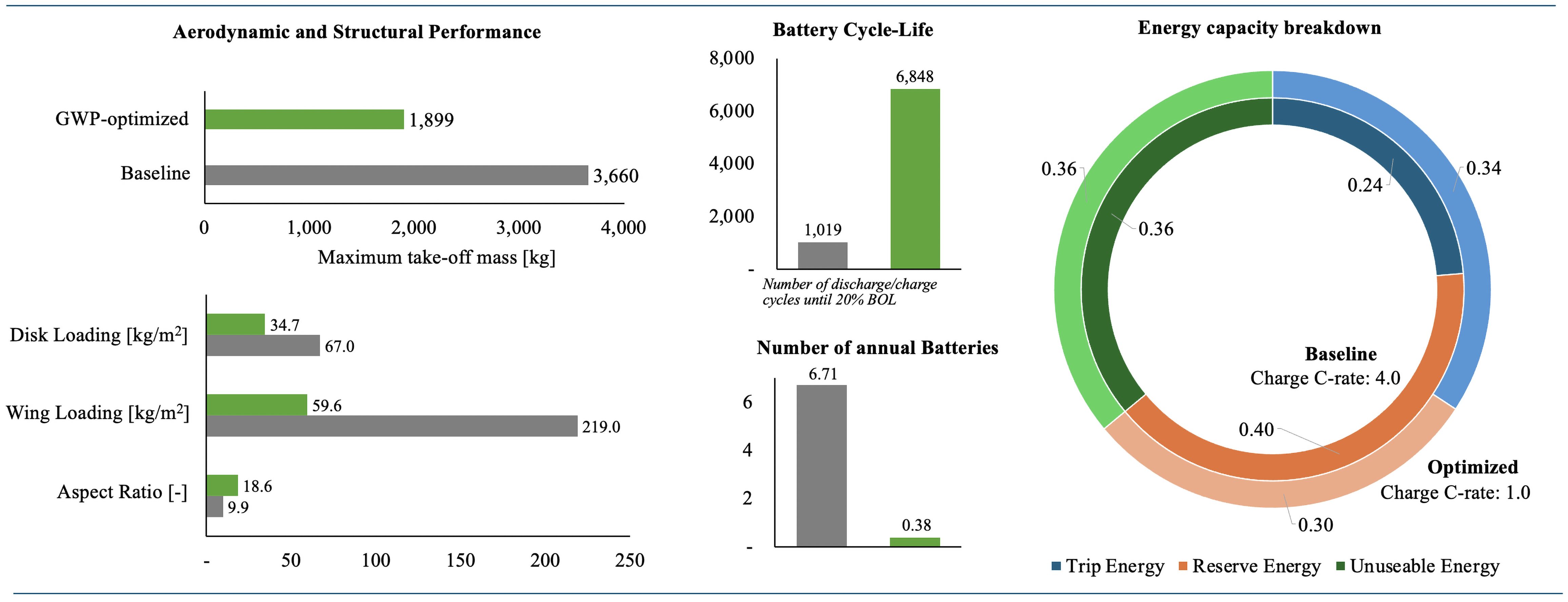
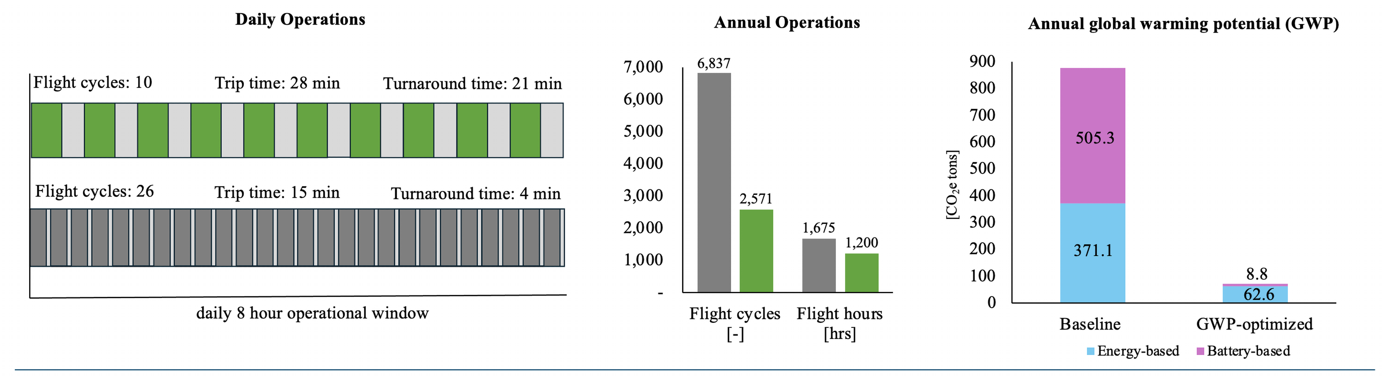
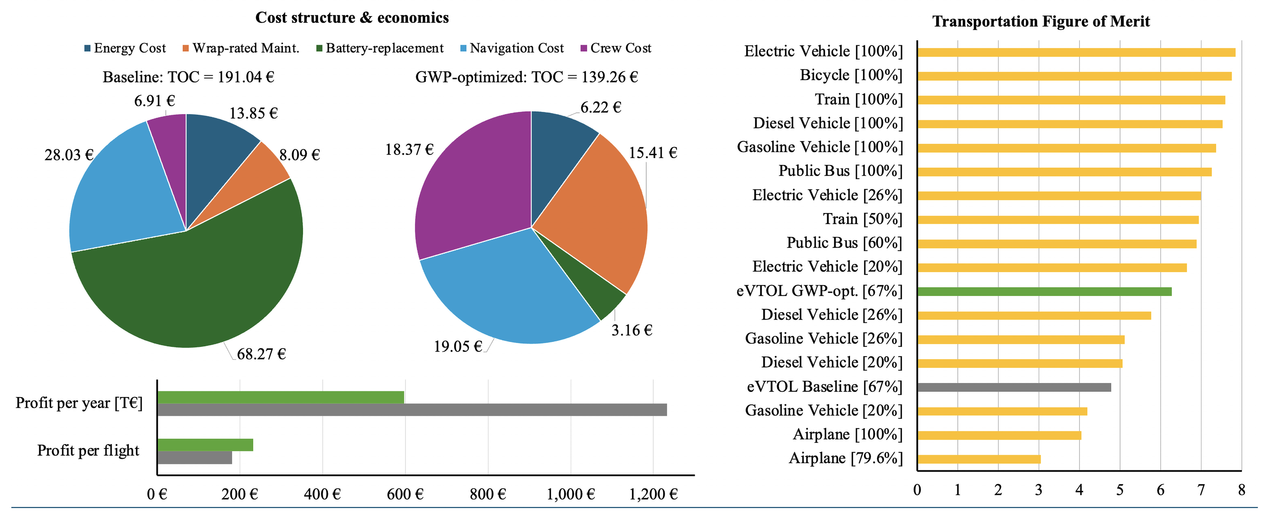
Figure 7: Comparative results of GWP-optimized eVTOL design.

The GWP-optimized design, achieving the lowest global warming potential shown in Figure 8, is characterized by a scenario of open vertiports, open rotor radii, high energy density of 400 Wh/kg, and a gentle 1C charging strategy, ensuring minimal environmental impact. As shown in Figure 12(c), this design prioritizes minimizing GWP by focusing on strict energy efficiency while adapting the aircraft’s components as required. The Pareto front analysis of Figure 12(c) highlights a key trade-off: while minimizing energy consumption (60-70 kWh) results in the lowest GWP, it also significantly increases required trip time, indicating inefficiencies at these low energy levels. Increasing energy consumption to around 90 kWh improves trip time but leads to a linear rise in GWP, emphasizing the delicate balance between environmental impact and operational efficiency.

The proposed design achieves a remarkable 92% reduction in annual GWP compared to the baseline, largely due to a 94% reduction in battery usage, from 6.7 to 0.38 batteries per year. The increase in battery cycle life—from 1,019 to 6,848 cycles—is driven by gentle 1C charging and a 24% reduction in average discharge C-rate due to efficiency improvement in each flight phase. Although the Depth of Discharge (DoD) increases by 43%, the overall required battery capacity is reduced by 69%. This allows for significant gain in energy usage efficiency, as now 34% instead of 24% of battery capacity is used for normal operation, and 30% instead of 40% battery capacity for reserve. 36% of the total battery capacity remain unusable, accounting for end-of-life and charging ceilings. A 48% reduction in MTOM, driven by a 77% decrease in battery mass and a 24% reduction in empty weight, plays a critical role in lowering energy requirements. However, the design’s larger rotor diameters of 2m and increased wing span — while improving flight efficiency due to high AR — also double the wing mass fraction and increase the gear mass fraction by a third. The aspect ratio of 18.6 significantly reduces wing and disk loading, resulting in a two-thirds reduction in power requirements. The design’s comparably low cruise speed, halved to 40 m/s (144 km/h) with respect to the baseline, further cuts energy requirements and negatively impacts operational performance. The 49% reduction in cruise speed has substantial operational consequences, increasing travel time by 91%, from 15 to 28 minutes, while extending turnaround time from 4 to 21 minutes due to the slow 1C charging rate. As a result, daily flight cycles drop by 62%, from 26 to 10, which directly reduces annual profit by 52%. Despite this, the design offers a 27% reduction in total operating costs compared to the baseline, with cash operating costs reduced by 50% and cost of ownership lowered by 24% due to a 24% decrease in aircraft acquisition costs. Energy costs fall by 55%, and battery replacement costs drop by a remarkable 95% due to gentle battery management, now accounting for only 2% of COC. However, time-dependent costs, particularly crew costs, rise significantly by 166%, from 6.91€ to 18.37€ per trip, due to the longer flight times. While the GWP-optimized design reduces TOC, the drop in flight cycles limits profitability, thus commercial viability. There is potential for profit recovery through modest increases in cruise speed or by reducing turnaround time via battery swapping. These adjustments could enhance operational efficiency without compromising the environmental benefits. The GWP-optimized design excels in minimizing environmental impact, achieving the highest GWP rating among all optimized designs as illustrated in Figure 9(b). Despite the reduced cruise speed, it maintains a strong time rating, indicating it remains faster than other non-eVTOL transportation modes. However, its cost rating is less competitive, particularly when compared to profit-optimized and TOC-optimized designs, reflecting the major trade-off between environmental sustainability and economic viability.

4.5 Results and Discussion of the Transportation FoM-maximizing eVTOL Design

The FoM-optimized design, achieving the highest overall transportational Figure of Merit, shown in Figure 8, is realized in a scenario which is characterized by open vertiports, open rotor radii, improved energy density, and a slow charging strategy, ensuring a balanced approach to operational efficiency, environmental impact, and economic viability. The corresponding Pareto front is shown in Figure 12(d), paired with the curve of FoM values for each design. In contrast to the previously discussed designs that strictly minimize energy or costs, this design strikes a balance, where slight increases in energy consumption lead to significant improvements in overall performance. The analysis shows that minimal energy usage results in unexpectedly high total operating costs, reducing the FoM. The FoM peaks at an energy levels slightly above the minimum, where TOC begins to decrease without excessively compromising GWP. This balance is achieved by avoiding the inefficiencies associated with extreme energy reductions, which drive up costs without proportional benefits. The FoM, therefore, represents an equilibrium where operational efficiency, environmental impact, and cost-effectiveness are optimized simultaneously. This approach positions the FoM-maximized design as the most competitive design strategy compared to other transportation modes, particularly when a balance between travel time, GWP, and costs is essential. The FoM-maximized design leverages the benefits of both TOC and GWP-optimized designs. It achieves an 89% reduction in GWP through strategies similar to the GWP-optimized design, such as increasing battery cycle life and improving flight efficiency. The use of a 1C charging strategy significantly reduces the number of batteries required, thereby lowering unit costs. Structurally, the design features a slightly increased aspect ratio, extending the wingspan to approximately 16 meters, which reduces wing loading. The increased rotor diameter to 2m decreases disk loading, contributing to more efficient flight. Overall, the aircraft’s weight is reduced by 48%, which is a critical factor in achieving these performance improvements.

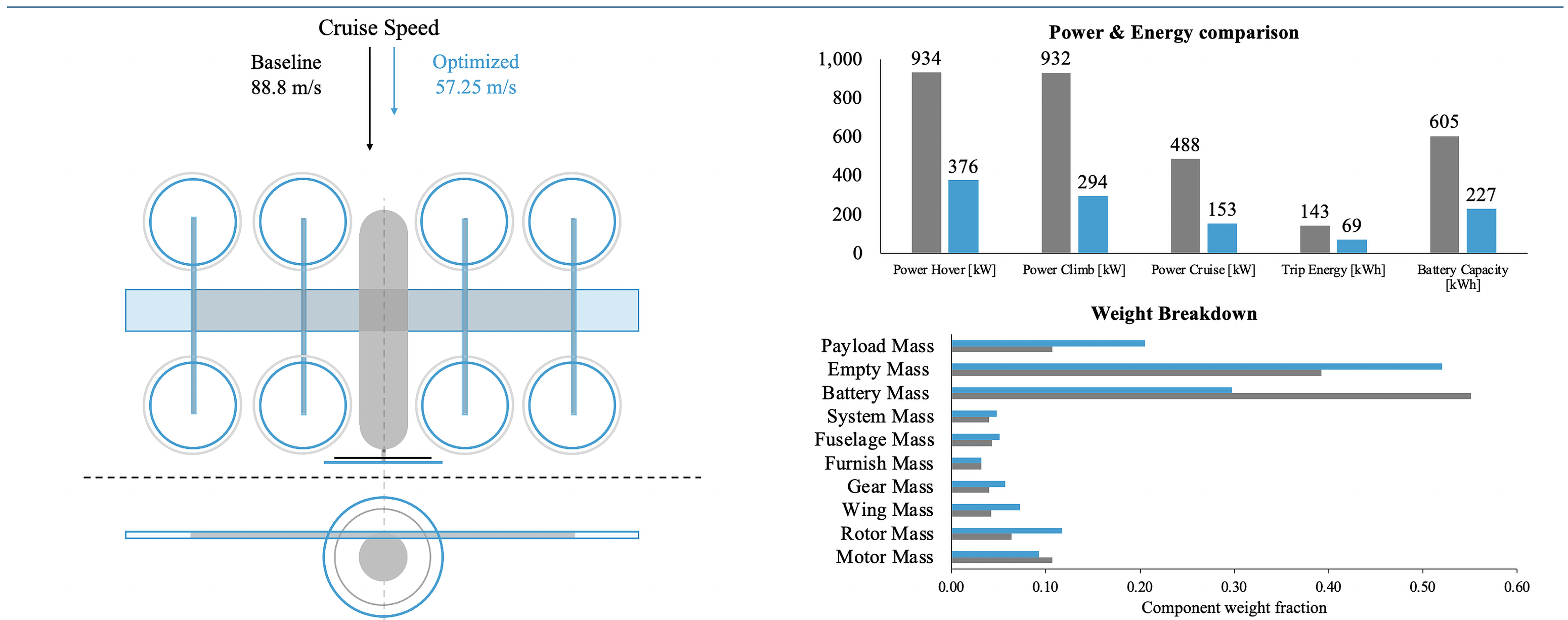
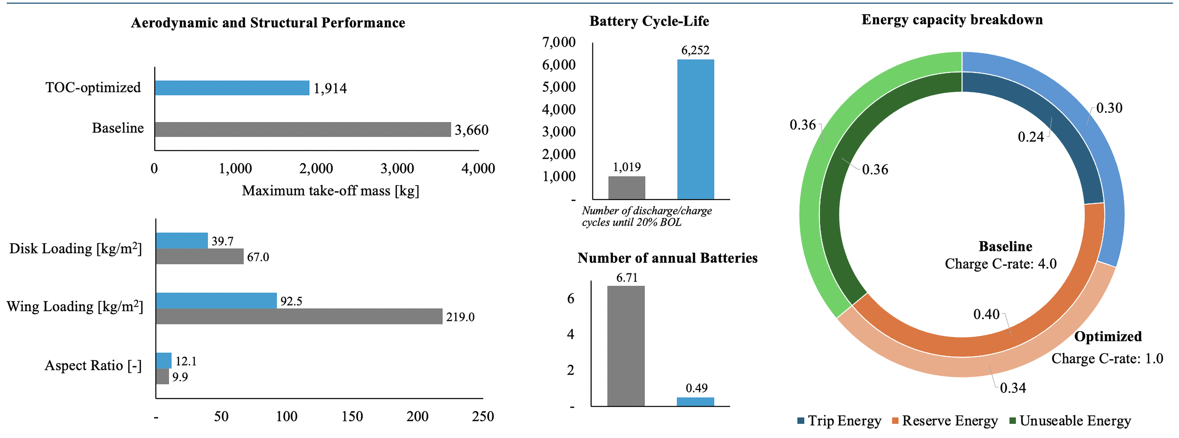
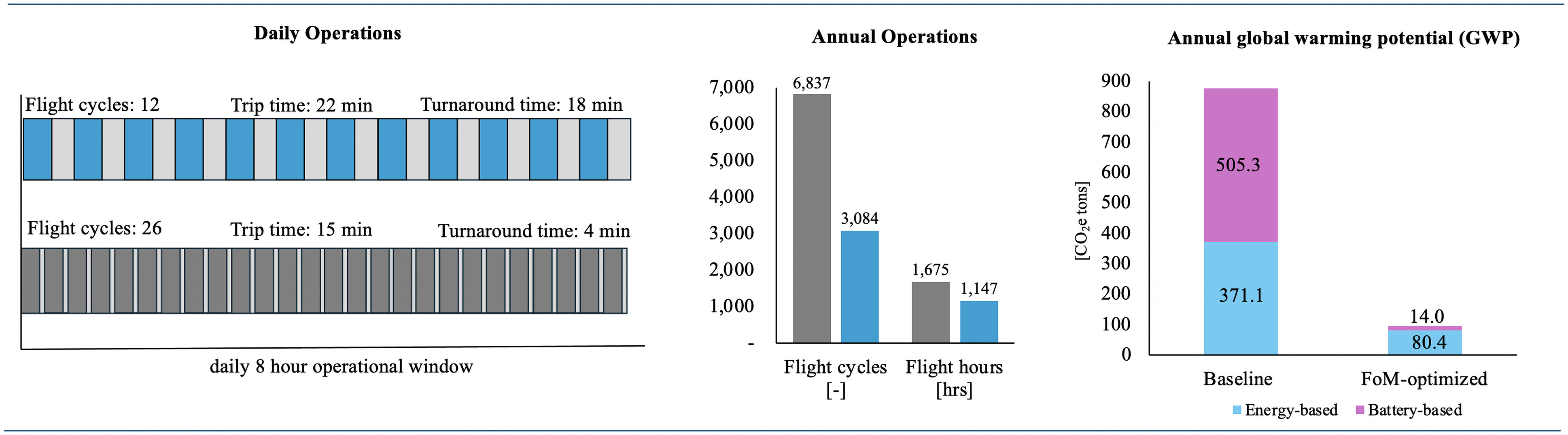
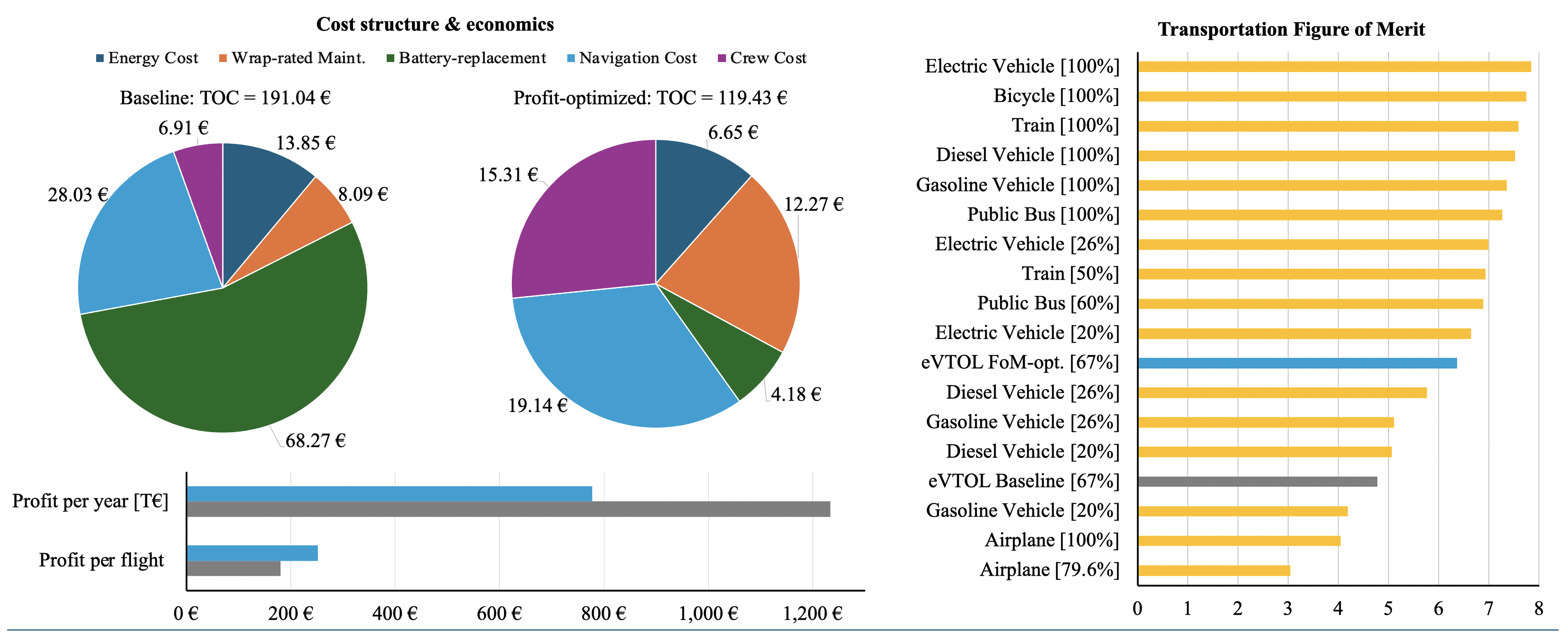
Figure 8: Comparative results of FoM-optimized eVTOL design.

The design achieves a 37% reduction in TOC, driven by a 94% decrease in battery replacement costs. However, like the GWP-optimized design, it experiences a significant increase in crew costs (122%) due to extended flight times. The FoM-maximized design also reflects the trade-off between per-flight profit, which can increase by 40%, and annual profit, which decreases by 37% due operational inefficiencies. This reduction in annual profit is primarily due to operational trade-offs, such as a 52% increase in travel time, an increase in turnaround time from 4 to 18 minutes, and a 55% reduction in daily flight cycles to 12. To address these operational challenges, minimizing turnaround time is critical. Implementing battery swapping could achieve this, increasing daily flight cycles and improving profitability, making specialized eVTOL designs more viable for real-world applications.

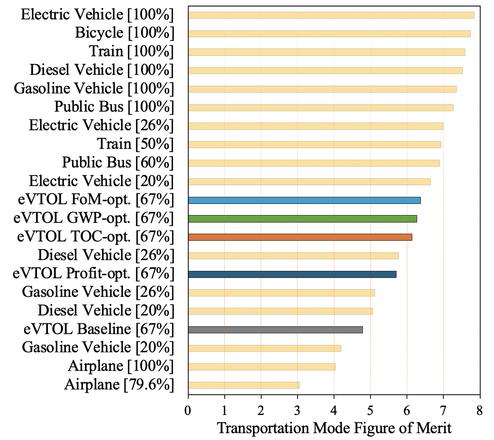
(a) Figure of Merit of specialized eVTOL designs.

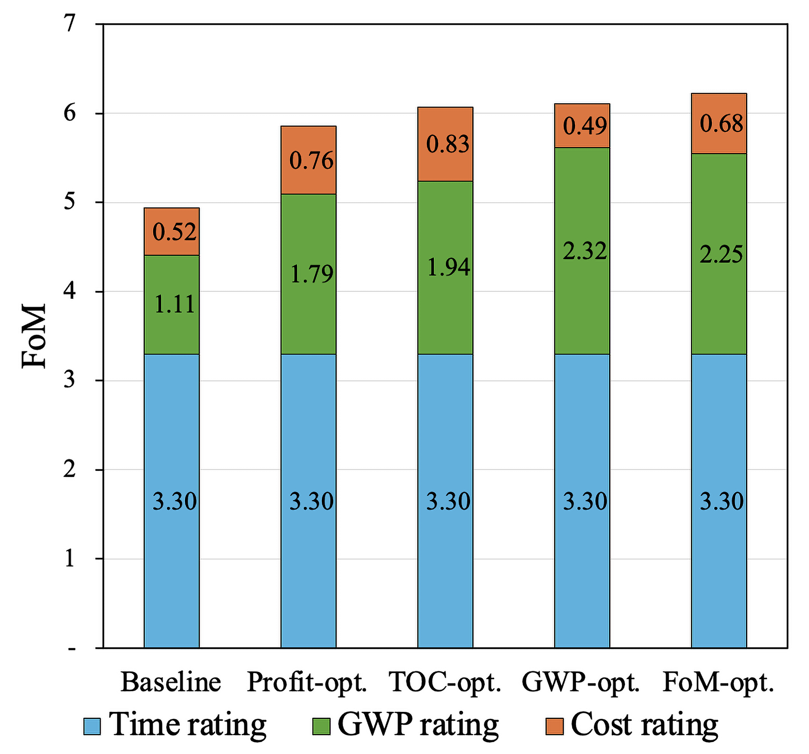
(b) Detailed FoM ratings for specialized designs.

Figure 9: Comparison of FoM metrics for different designs and transportation modes.

4.6 Baseline-relative comparison of results

Figures 10 and 11 show relative comparative results data for each design in relation to the baseline design. Figure 10 illustrates the airframe design-specific characteristics of our proposed eVTOL designs. Figure 11 contains the relative data on battery and GWP differences, as well as operation and economic performance of the designs.

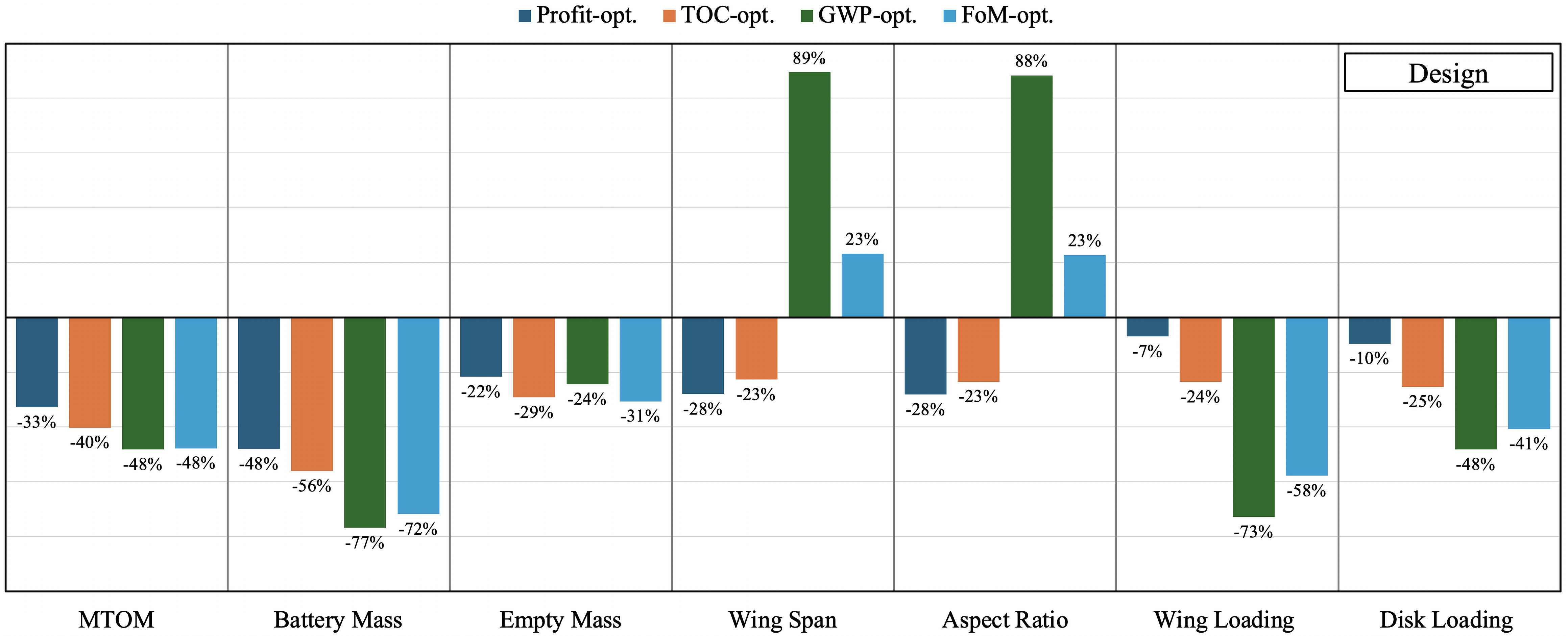
Figure 10: Relative design metrics of specialized eVTOL designs in comparison to baseline.

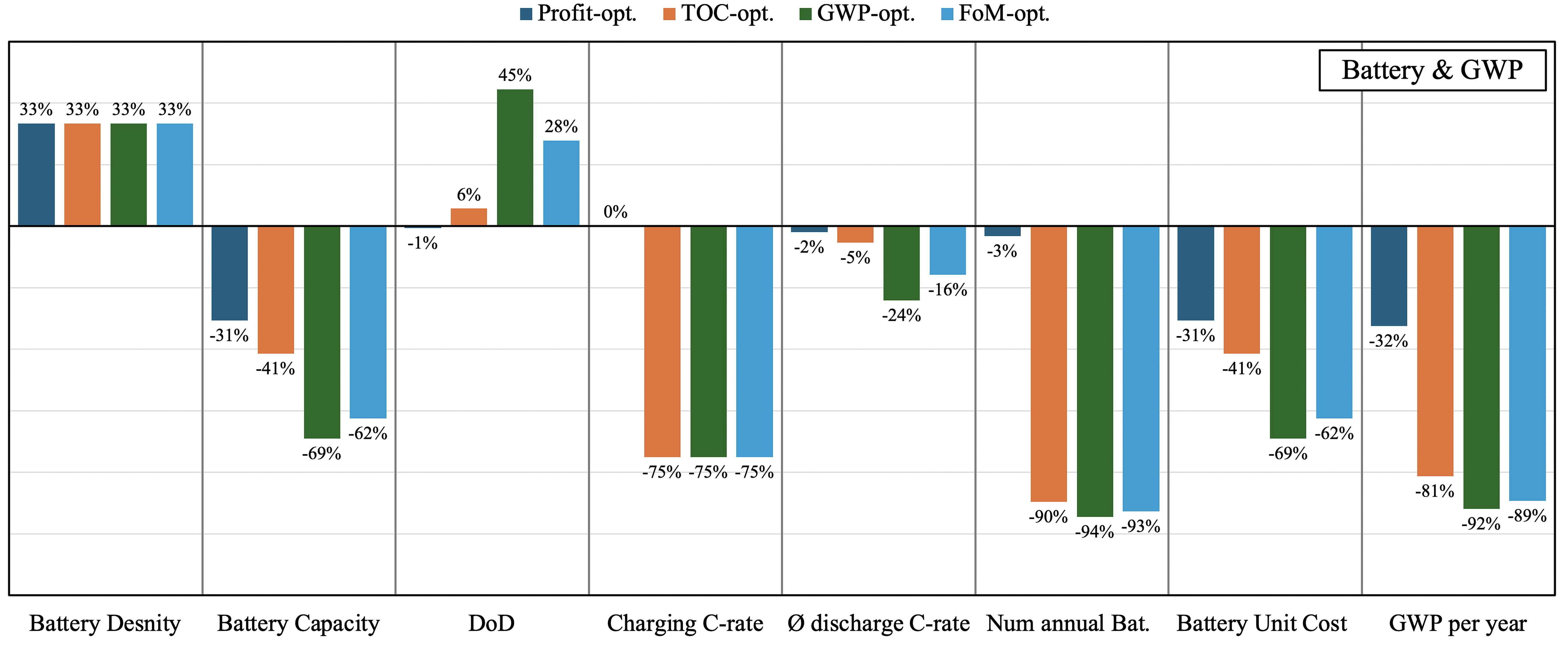
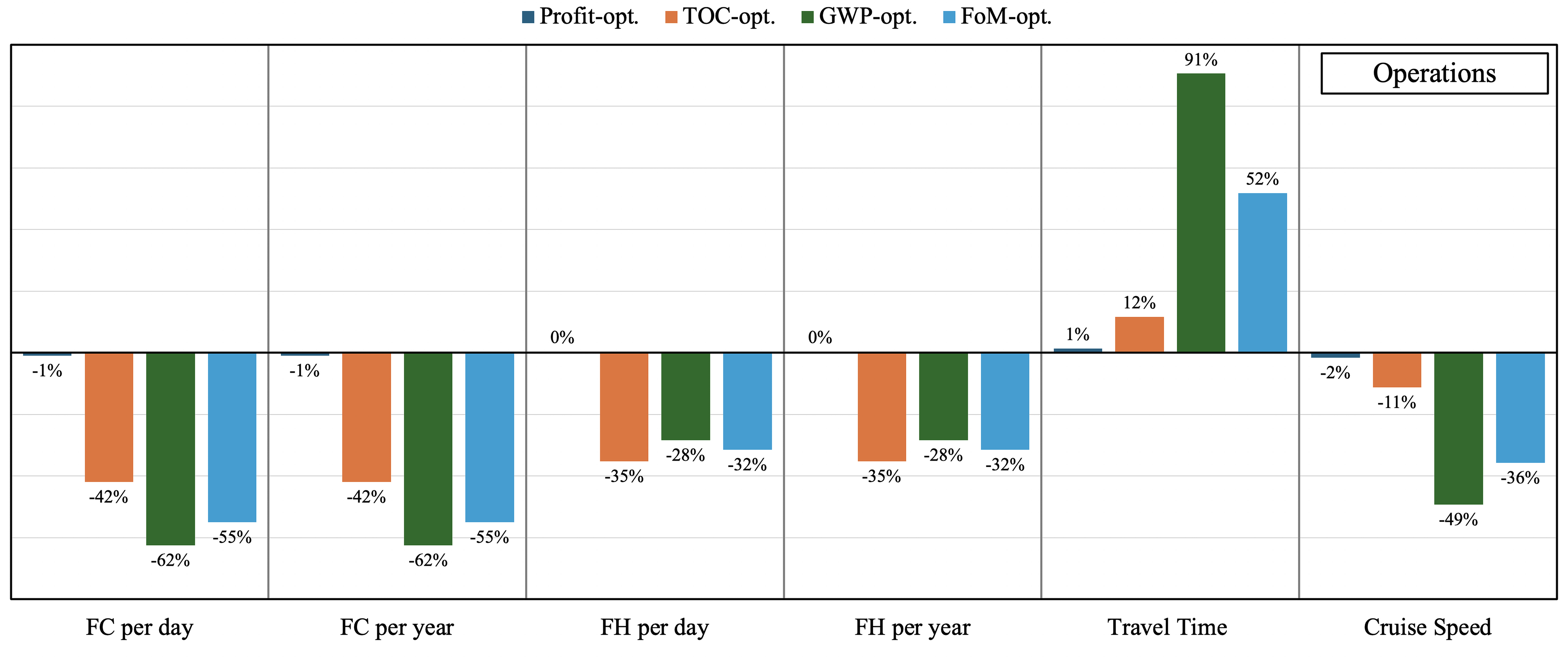
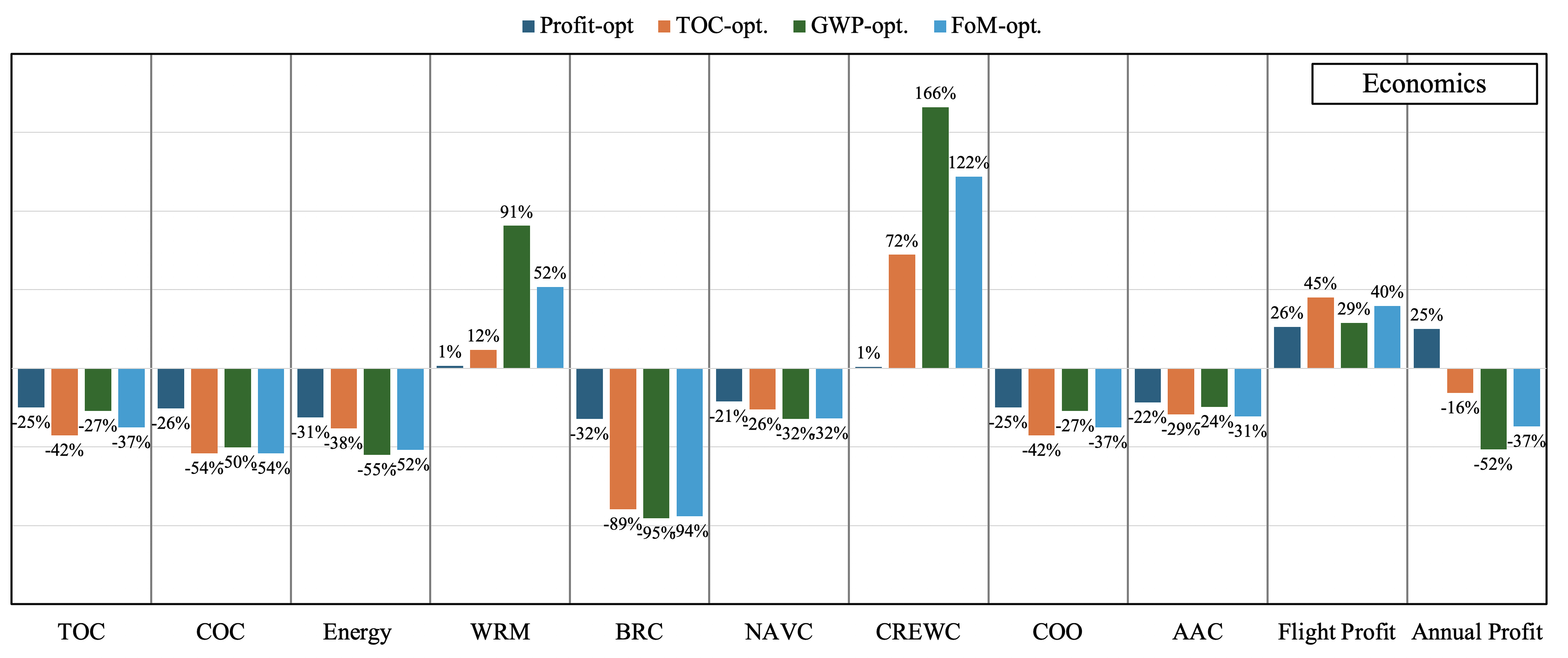
Figure 11: Relative performance metrics of specialized eVTOL designs in comparison to baseline.

4.7 Strategic Trade-Offs in Specialized eVTOL Designs

The analysis of specialized eVTOL designs — optimized respectively for maximum profit, minimum TOC, minimum GWP, and maximum FoM — reveals critical insights into the trade-offs that stakeholders must consider when selecting or developing aircraft for regional (RAM) and urban air mobility (UAM). Each design offers distinct advantages tailored to specific operational priorities, but these benefits often come with significant drawbacks that may limit their practicality in a broader market context. Figure 12 (a) to (d) each describe the design space of an eVTOL, characterized by the respective pareto front (in black), which describes the general trade-off between trip time (y-axis) and energy demand (x-axis). As a decision-making tool for determining the respective object-specific optimized design, the target value calculated for each pareto point ((a) annual profit (dark blue), (b) total operating cost per trip (orange), (c) annual GWP (green), (d) Figure of Merit (light blue)) is plotted over the pareto front.

(a) Max. profit design on pareto front.

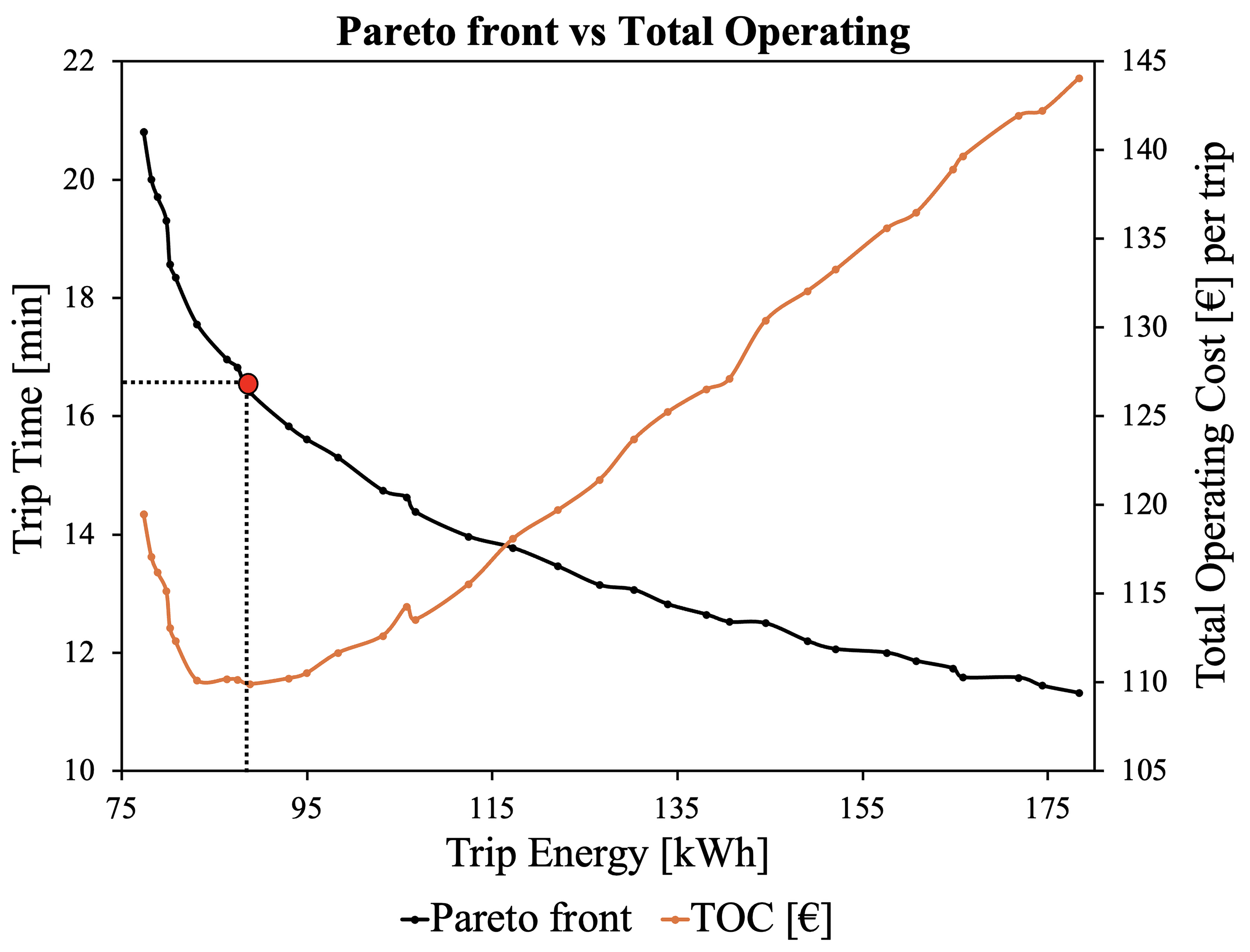
(b) Min. TOC design on pareto front.

(c) Min. annual GWP design on pareto front.

(d) Max. FoM design on pareto front.

Figure 12: Localization of trade-offs in specialized eVTOL designs: The red dot indicates the optimal eVTOL design on the pareto front (black curve). The colored curves illustrate the associated objective metric used to guide decision-making for the optimal design.

4.8 Validation against Uber UAM Requirements

This section evaluates how the specialized eVTOL designs align with Uber’s UAM requirements, illustrated in Table 5, to assess economical use of the proposed designs. The focus is on key differences and similarities in terms of vehicle performance, economic competitiveness, with implications for UAM operations and design optimization.

	Uber Elevate [23]	Profit-opt.	TOC-opt.	GWP-opt.	FoM-opt.
Vehicle Design and Performance
Maximum take-off mass [kg]	1,814.40	2,458.98	2,187.30	1,898.78	1,913.54
Battery specific energy [Wh/kg]	400	400	400	400	400
Battery cycle life [cycles]	2,000	1,043	5,667	6,848	6,252
Battery capacity [kWh]	140	419	355	188	227
Cruise speed [km/h]	320	315	285	163	206
Motion efficiency at cruise [km/kWh]	1.24	0.71	0.79	1.09	1.02
Power required at hover [kW]	500	597	482	349	376
Power required at cruise [kW]	120	339	277	112	154
Lift-to-drag ratio [-]	13	9	9	12	11
Economic Competitiveness
Cost per pax-kilometer [€/km]	0.27	0.51	0.39	0.50	0.43
Cost per pax-minute travelled [€/min]	1.27	3.59	2.50	1.85	2.00
Cost of a 70 km pooled VTOL trip per person [€]	19	36	27	35	30
Vehicle utilization (hours per year)	2,080	1,682	1,086	1,200	1,147
Load factor (average seats filled)	67%	67%	67%	67%	67%
Operational Costs
Piloting cost as % of direct operating costs	36%	6%	15%	21%	19%
Maintenance costs as % of direct operating costs	22%	46%	21%	21%	21%
Battery costs as % of direct operating costs	2%	39%	9%	4%	5%
Energy cost costs as % of direct operating costs	12%	8%	11%	7%	8%
Ownership costs as % of direct operating costs	8%	22%	26%	29%	27%

Table 5: Summary of Uber eVTOL UAM requirements and comparison.

Uber’s requirements emphasize motion efficiency and operational capability. The profit-optimized design, with its higher take-off mass (2,459 kg) and battery capacity (419 kWh), shows the lowest motion efficiency (0.71 km/kWh) and the highest power demands in both hover (597 kW) and cruise (339 kW), deviating significantly from Uber’s target of 1.24 km/kWh. Additionally, this design has the shortest battery cycle life, leading to the highest battery and maintenance costs among all designs. It is evident that gentle charging strategies, such as those using a 1C rate, substantially increase battery cycle life. The GWP and FoM-optimized designs align more closely with Uber’s baseline in terms of MTOM. The GWP-optimized design achieves lower cruise power requirements than Uber’s target, albeit with a significant reduction in cruise speed. In contrast, the FoM-optimized design strikes a balance between cruise speed and power requirements, offering a more rounded approach. However, none of the designs meet the required 2,080 flight hours per year, with the profit-optimized design reaching only 1,682 hours, approximately 400 hours short of the target. This shortfall in flight hours could impact service availability and necessitate a larger fleet to meet demand, potentially driving up operational costs. Regarding costs per seat, which Uber sets at €19 for a typical trip, the TOC-optimized design achieves the lowest cost among the specialized designs at €27. This indicates that further significant cost reductions are necessary to meet Uber’s stringent economic goals. Potential cost savings are particularly apparent in ownership costs, which are tied to aircraft acquisition expenses. These costs are expected to decrease as production scales, potentially reducing overall operating costs in the long term. Additionally, improvements in battery technology, such as higher specific energy or faster charging methods beyond 1C, could further shift the economic balance, making these designs more viable. Overall, all designs fall within reasonable limits and are broadly aligned with Uber Elevate’s requirements, suggesting potential real-world viability. The economic feasibility and operational implementation of these designs merit further research to ensure they can meet the demands of urban air mobility. Moreover, while the environmental benefits of the GWP-optimized design are clear, further assessment is needed to evaluate how these designs align with Uber’s broader sustainability strategy, particularly in terms of long-term environmental impact and scalability. This comparison illustrates that potential future large scale UAM operators such as Uber are aiming for a hard balance in operational efficiency, such as high cruise speed at low power requirements combined with high demands in cost efficiency.

5 Conclusion

Our multidisciplinary design optimization framework provides a platform for analyzing and optimizing technological, environmental, and economic interdependencies of the eVTOL ecosystem. The analysis of the specialized eVTOL designs provides important insights to address complex trade-offs between these domains, necessary to be considered by UAM stakeholders. Our results provide an in-depth assessment of four specialized eVTOL designs, each optimized for different objectives: maximum profit, minimum total cost of ownership (TOC), minimum global warming potential (GWP), and maximum figure of merit (FoM). The main conclusions from our work and UAM stakeholder strategies and recommendations are as follows:

A profit-optimized eVTOL design achieves substantial operational efficiency gains through short travel times and minimized turnaround and battery recovery times, yet its long-term sustainability is hindered by the environmental impact of current battery technologies, highlighting the need for advancements in battery recycling. In contrast, a TOC-optimized design maximizes cost efficiency but sacrifices operational flexibility and profitability, underscoring the importance of balancing cost minimization with operational performance metrics. A GWP-optimized design, while significantly reducing environmental impact, faces limitations in economic viability due to extended travel times and reduced flight cycles, as energy consumption-optimized airspeed and a battery charging management system tailored to longevity are decisive factors. Finally, an inter-transportation-modal, FoM-maximized design provides a balanced design approach based on passenger preferences and comparability with ground transportation alternatives. This approach integrates cost efficiency, operational performance, and sustainability to provide a comprehensive solution for urban air mobility requirements.

Slow charging extends battery life and reduces the frequency of replacement, which reduces long-term costs and improves sustainability, as shown in the scenario for minimum GWP- and maximum FoM-eVTOL design. Despite increased turnaround times and potential losses in operational efficiency, the cost and ecological advantages outweigh the disadvantages. Battery swapping stations allow for quick replacement of discharged batteries at vertiports, reducing downtime and maximizing daily flight cycles. This increases profitability through more frequent flights, but comes with risks such as high investment costs, complex inventory management, and the need for standardized eVTOL designs. The regulatory and logistic challenges of integrating battery swapping and charging stations should be addressed in future work.

Removing vertiport dimension limitations allows for optimized eVTOL designs with larger wingspans and rotor diameters, improving aerodynamic efficiency, reducing energy consumption, and lowering costs. However, flight efficiency-optimized eVTOL designs are reaching the limits of existing helipads. Adaptive wing technologies, such as Airbus’ Extra Performance Wing demonstrator [45], offer a solution by utilizing foldable and movable wings that both improve aerodynamics and ensure infrastructure compatibility. This innovation enables efficient use of existing landing sites, but increases technical complexity and requires careful consideration of certification.

In summary, a strategic focus on battery life extension, recycling processes, optimized vertiport utilization, and adaptive wing designs that combine efficient aerodynamic design with infrastructure compatibility is recommended. The further development of eVTOL technologies should be supported by life cycle analyses, precise noise modeling, and economic operational optimization. Close co-operation between industry and regulatory authorities is essential to make UAM sustainable and economically viable.

6 Supplementary Material

The source code and industry design comparison file is available on github.com/JohannesJanning.

Appendix A Appendix: Key Design Metrics

Key Metrics	Description
MTOM ($kg$)	Crucial metric that represents the total mass the aircraft is designed to carry, including the aircraft itself, passengers, cargo, and batteries. It directly impacts performance, range, and regulatory compliance.
Empty Mass ($kg$)	Includes the weight of the aircraft without any payload or battery. A lower empty mass generally indicates a more efficient design, potentially allowing for more payload or longer range and reduced aircraft acquisition cost.
Wing Mass ($kg$)	Contributes significantly to the overall structural weight. It affects the aircraft’s balance, structural integrity, and aerodynamic performance. Optimizing wing mass is crucial for maintaining a balance between strength and weight efficiency.
Battery Mass ($kg$)	Critical in electric aircraft, as it directly impacts range, endurance, and overall energy efficiency. A heavier battery can provide more energy but may reduce efficiency and payload capacity.
Aspect Ratio ($-$)	Key indicator of aerodynamic efficiency. A higher aspect ratio typically leads to lower drag, improving fuel efficiency and range.
Wing Loading ($kg/m^{2}$)	Affects the aircraft’s performance in terms of takeoff, landing, and maneuverability. It’s a critical factor in determining how the aircraft behaves under different flight conditions.
Disk Loading ($kg/m^{2}$)	Important for vertical take-off and landing (VTOL) performance. Lower disk loading generally improves hover efficiency and reduces the power required for lift.

Table 6: Aircraft Design Key Metrics Overview.

Key Metrics	Description
GWP per Flight ($CO2_{e}kg$)	Measures the total CO2 equivalent emissions generated by the aircraft during a single flight. It’s crucial for assessing the direct environmental impact of each operation, allowing to evaluate how sustainable each design is on a per-flight basis, providing a clear understanding of the environmental footprint of individual operations.
GWP per Year ($CO2_{e}kg$)	Aggregates the total CO2 equivalent emissions for all flights over a year. It’s essential for understanding the long-term environmental impact of the eVTOL operations for evaluating sustainability in the context of regulatory compliance and corporate environmental goals.
GWP per Passenger Kilometer ($CO2_{e}kg/km$)	Normalizes the CO2 emissions by the distance traveled per passenger, making it easier to compare the environmental efficiency of different designs or transportation modes.
Energy per Kilometer (EpK) ($kWh/km$)	Measures the energy consumption of the eVTOL per kilometer traveled, allowing to assess how different designs optimize energy use, which is critical for both sustainability and cost efficiency.
Charging C-rate ($1/h$)	Indicates how quickly the battery can be recharged. Faster charging times are crucial for reducing turnaround times in operations but may affect battery longevity if not managed properly.
Trip Energy Required ($Wh$)	Measures the total energy consumed during a single flight. It’s a comprehensive metric that captures the energy demands of the entire operation, from takeoff to landing, providing a holistic view of the energy efficiency of each flight.

Table 7: Sustainability Key Metrics Overview.

Key Metrics	Description
Battery Density ($Wh/kg$)	Measures how much energy a battery can store relative to its weight. Higher energy density is desirable because it allows for longer flight times and greater range without significantly increasing the aircraft’s weight.
Battery Capacity ($kWh$)	Determines the total amount of energy available for a flight. It directly impacts the range and endurance of the eVTOL. A higher capacity allows for longer trips but usually results in a heavier battery, affecting overall efficiency.
Depth of Discharge (DoD)($\%$)	Indicates the percentage of the battery’s total capacity that is used during a discharge cycle. Managing DoD is crucial for balancing range with battery longevity; deeper discharges can shorten battery life, while shallower discharges may limit range.
Average Discharge C-rate ($1/h$)	Measures how quickly a battery is discharged relative to its capacity. The average discharge C-rate provides insight into the battery’s performance during a typical flight. High C-rates can stress the battery, potentially reducing its lifespan, but may be necessary for high power demands.
Charging C-rate ($1/h$)	Indicates how quickly the battery can be recharged. Faster charging times are crucial for reducing turnaround times in operations but may affect battery longevity if not managed properly.
Number of Battery Cycles ($-$)	Measures the number of complete charge/discharge cycles the battery can undergo before its capacity significantly degrades. It’s a critical factor in determining the overall lifespan of the battery and impacts the cost-efficiency of operations.
Number of Yearly Required Batteries ($-$)	Estimates how many batteries are needed per year to maintain operations, accounting for factors like battery wear and the number of cycles. It’s essential for understanding operational costs, planning maintenance and estimating total global warming potential (GWP) of the eVTOL operation, due battery life-cycle environmental impact.
Battery Unit Cost (€)	Key economic metric that influences the overall maintenance cost and operation. Lower battery costs are preferable, especially if batteries need frequent replacement.

Table 8: Battery Design Key Metrics Overview.

Key Metrics	Description
Flight Cycles per Day ($-$)	Measures the number of complete flights an eVTOL can perform daily while indicates daily operational capacity and utilization; higher values suggest better efficiency.
Flight Cycles per Year ($-$)	Total number of flights over a year. Reflects long-term operational workload, impacting maintenance and lifecycle costs.
Flight Hours per Day ($hrs$)	Total time the eVTOL spends in the air each day, providing a measure of daily operational tempo and productivity.
Flight Hours per Year ($hrs$)	Aggregated flight time over a year. Key for planning maintenance and understanding long-term aircraft usage.
Travel Time ($min$)	Total time for a complete trip, including takeoff, cruise, and landing. Shorter travel times may improve customer satisfaction and operational efficiency.
Turnaround Time Between Trips ($min$)	Assumed as time needed to prepare the eVTOL for the next flight, including charging. Shorter turnaround times maximize flight availability and operational efficiency.
Cruise Speed ($km/h$)	Directly impacts the duration of the flight, the efficiency of the operation, and the scheduling of trips. It affects how quickly the eVTOL can complete a journey, which in turn influences the number of trips it can perform within a given time period and also determines eVTOL power requirements.
Power in Hover ($kW$)	Measures the power required to maintain a hover, critical for VTOL operations, crucial for urban operations.
Power in Climb ($kW$)	Measures the power needed during the climb phase, which is typically energy-intensive.
Power in Cruise ($kW$)	Measures the power required to maintain cruise speed. It’s crucial for understanding energy efficiency during the longest phase of flight.

Table 9: Operational Key Metrics Overview.

Key Metrics	Description
Total Operating Cost (€)	Captures all costs associated with operating the eVTOL for one trip, providing an overall measure of economic efficiency per flight.
Cash Operating Cost (€)	Focuses on the cash expenses incurred during each flight. Useful for understanding immediate financial outflows directly related to eVTOL operation.
Energy Cost (€)	The cost of energy consumed during a single trip, directly linked to the aircraft’s energy efficiency and the operator’s regional electricity mixture network.
Warp Rated Maintenance (€)	Estimated maintenance costs, considering wear and tear per trip.
Battery Replacement Cost (€)	Cost allocated for battery replacement, spread over the battery’s life.
Navigation Cost (€)	Expenses related to navigation services during the flight, containing air traffic service charges.
Crew Cost (€)	Wages for the flight crew per trip.
Cost of Ownership (€)	Total cost of owning and operating the eVTOL, divided per trip. Provides a comprehensive view of long-term financial commitments.
Aircraft Price (€)	Estimated initial purchase price of the eVTOL. Key for calculating depreciation and understanding capital investment.
Profit per Flight (€)	Revenue minus costs for each flight. Direct measure of economic performance per operation.
Annual Profit (€)	Total profit accumulated over a year. Crucial for assessing the long-term viability and success of the eVTOL operation, depending on operational metrics.

Table 10: Economic Key Metrics Overview.

Appendix B Appendix: Model Documentation

B.1 Mass Model

B.1.1 Maximum Take-Off Mass

Assumptions and Limitations:

• Due to the preliminary design nature of the optimisation, MTOM should be treated as a first estimate.

• The proposed design optimization allows a deviation by 2% of eq. 24.

The total mass of an eVTOL aircraft can be generally described by (expressed in kg):

$$MTOM=M_{payload}+M_{empty}+M_{battery}\leq Limit_{certification}$$ (24)

with $MTOM$ being the maximum take-off mass, $M_{payload}$ the payload mass, $M_{empty}$ the empty mass, and $M_{battery}$ the battery mass. According EASA’s latest certification specifications for eVTOL, Ref. [29], the maximum certifiable weight is limited to $Limit_{certification}=5.700kg$.

B.1.2 Battery Mass

Assumptions and Limitations:

• Battery Mass accounts for design mission energy requirements, as sum of reserve and trip energy. Reserve energy can be adjusted by the user by selecting reserve time, which is assumed to be 30min in cruise power.

• 20$\%$ of unusable battery capacity in terms of state of charge ceiling and floor are considered (see Chapter B.3.6).

• The end-of-life battery status is considered, defined by 80$\%$ of begin-of-life condition (see Chapter B.3.6).

Historically, $M_{battery}$ would be considered as part of $M_{empty}$, but for enormous impact of $M_{battery}$ on MTOM, it is considered separately. $M_{battery}$ can be calculated by eq. 25, considering the design mission energy needs and battery energy density $\rho_{bat}$ in Wh/kg. The factor of $0.64$ accounts for unusable battery energy (see Chapter B.3.6).

$$M_{battery}=\frac{E_{useable}}{e_{usable}}=\frac{E_{trip}+E_{res}}{0.64\cdot\rho_{bat}}\left[{kg}\right]$$ (25)

B.1.3 Payload

Assumptions and Limitations:

• Payload is defined by load factor, number of passengers and their average mass.

• Within this framework a constant payload and a load factor of 1 is considered, according equation 27.

$M_{payload}$ should count for an average passenger weight $M_{pax}$ and luggage weight per passenger $M_{lug}$. The mean Passenger and Luggage weights for commercial air transportation are assumed $M_{pax}$=82.2kg and $M_{lug}$=16kg [32]. $n_{seats}$ is the maximum seat capacity of the aircraft. LF is the load factor of the aircraft.

$$M_{payload}=(M_{pax}+M_{lug})\cdot n_{seats}\cdot LF$$ (26)

In a fully loaded 4-seater eVTOL this results in:

$$M_{payload}=(82.2+16)\cdot 4\cdot 1=392.8\left[{kg}\right]$$ (27)

B.1.4 Empty Mass

Assumptions and Limitations:

• This method is used within the presented optimization.

• Statistical methods highly depend on the used data set for model fit. The provided methods are based on general aviation aircraft.

• The provided equations are highly unit sensitive. Use the provided conversion table to transfer metric units into imperial units, insert the imperial units into the models and re-transfer the results from pounds to kilogram.

• Wihtin this framework, statistical mass estimations according Raymer [30] and Nicolai [31] are averaged.

The empty mass in this method is defined as:

$$M_{empty}=M_{wing}+M_{rotor}+M_{motor}+M_{fuselage}+M_{systems}+M_{furnish}+M_{crew}$$ (28)

Where crew mass $M_{crew}$ is based on average masses for single pilot operation [32]. Within this method, the values in Table 11 are used for unit conversion.

Unit	Metric	Imperial
Weight	1 kg	2.20462 lb
Length	1 m	3.28084 ft
Area	1 m2	10.7639 ft2
Speed	1 m/s	1.94384 kt

Table 11: Conversions from Metric to Imperial Units

B.1.5 Wing Mass

Assumptions and Limitations:

• Within optimization model, rectangular wing with NACA2412 airfoil is assumed, taper ratio $\lambda$ is assumed 1 and sweep angle $\Lambda_{c/4}$ to be 0°.

• Airfoil data for NACA0012 is provided in Chapter B.2 and can be adjusted in the provided optimization code.

• Thickness to chord $t/c$ ratio is assumed for 0.12 (NACA2412).

• Maximum level airspeed $V_{H}$ is assumed to equal $V_{cruise}$.

• The calculation of the wing mass is based solely on statistical mass estimation, based on historical aircraft data from general aviation. Detailed structural and geometric characteristics of the wings are not taken into account. The integration of a FEM model, for example, for a more accurate calculation of the wing mass, taking into account more precise wing design parameters, has the potential to significantly complement the proposed model in future work.

Raymer:

$$M_{W_{R}}=0.036\cdot S_{W}^{0.758}W_{FW}^{-0.0035}\left(\frac{AR_{W}}{\cos^{2}\Lambda_{C/4}}\right)^{0.6}q^{0.006}\lambda^{0.04}\left(\frac{100\cdot t/c}{\cos\Lambda_{C/4}}\right)^{-0.3}(n_{z}W_{O})^{0.49}$$ (29)

Nicolai:

$$M_{W_{N}}=96.948\cdot\left(\frac{n_{z}W_{O}}{10^{5}}\right)^{0.65}\left(\frac{AR_{W}}{\cos^{2}\Lambda_{C/4}}\right)^{0.57}\left(\frac{S_{W}}{100}\right)^{0.61}\left(\frac{1+\lambda}{2(t/c)}\right)^{0.36}\left(\sqrt{1+\frac{V_{H}}{500}}\right)^{0.993}$$ (30)

In the given equations:

• $M_{W}$ is the predicted weight of the wing in pounds-force (lbf).

• $S_{W}$ is the trapezoidal wing area in square feet (ft²).

• $W_{FW}$ is the weight of fuel in the wing in pounds (lbs) (if $W_{FW}=0$, then let $W_{FW}^{0.0035}=1$).

• $AR$ denotes the Aspect Ratio of the wing, HT, or VT, as per the appropriate subscripts.

• $\Lambda_{C/4}$ is the wing sweep at 25% Mean Geometric Chord (MGC).

• $q$ represents the dynamic pressure at cruise.

• $\lambda$ is the wing taper ratio.

• $t/c$ refers to the wing thickness to chord ratio.

• $n_{z}$ is the ultimate load factor.

• $W_{0}$ is the design gross weight in pounds (lbs).

• $V_{H}$ is the maximum level airspeed at Sea Level (S-L) in Knots Equivalent Airspeed (KEAS).

Resulting in:

$$M_{wing}=\frac{M_{W_{R}}+M_{W_{N}}}{2}$$ (31)

B.1.6 Rotor Mass

The rotor weight model from [6], which deals with UAM, was adopted and adapted for passenger transporting EVTOL using a correction factor. The average weight and radius of a series of MT propellers from Table 12, based on [46], was used as a reference to identify a matchpoint where the radius of 1.1m hits 18.0kg. In addition the model was damped by adjusting the potency of the disproportionality to moderate the exponential increase in rotor weight with rotor size.

$$M_{R}=k_{rotor}\cdot\left[n_{h}\cdot\left(0.7484\cdot R_{\text{hover}}^{1.2}-0.0403\cdot R_{\text{hover}}\right)+n_{c}\cdot\left(0.7484\cdot R_{\text{cruise}}^{1.2}-0.0403\cdot R_{\text{cruise}}\right)\right]$$ (32)

where $n_{h}$ and $n_{c}$ are the number of rotors in the hover configuration and cruise configuration, respectively. During climb, the cruise propeller is used. $R_{i}$ represents the radius of each propeller, with $i$ indicating either the hover or cruise configuration.

Type	MT-11	MT-15	MTV-21	MTV-17	MTV-20	Average
D [cm]	190	260	203	190	210
r [cm]	95	130	101.5	95	105	1.1
M [kg]	16	25	12	16	21	18

Table 12: Technical Data for MT Propellers

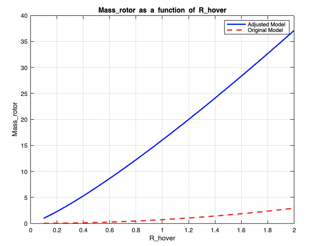
Figure 13: Rotor mass model.

B.1.7 Landing Gear Mass

Assumptions and Limitations:

• The provided equations are highly unit sensitive. Use the provided conversion table to transfer metric units into imperial units, insert the imperial units into the models and re-transfer the results from pounds to kilogram.

The Landing gear mass is computed by averaging statistical models. Raymer provides to equations, one for main landing gear and one for nose landing gear. Nicolai provides a model for the entire landing gear. The landing gear weight is driven by total aircraft mass $MTOM$ and length of the gear struts $L_{m}$ and $L_{n}$, summarized as $L_{i}$. $L_{i}$ is defined by the cruise propeller radius $R_{prop_{cruise}}$ and the minimum propeller clearance of 7 inches (0.1778m) as required by EASA, Ref. [47], and FAA, Ref. [48].

Raymer:

$$W_{MLG_{R}}=0.095\cdot(n_{l}\cdot W_{l})^{0.768}\left(\frac{L_{m}}{12}\right)^{0.409}$$ (33)

$$M_{NLG_{R}}=0.125\cdot(n_{l}W_{l})^{0.566}\left(\frac{L_{n}}{12}\right)^{0.845}$$ (34)

where:

• $W_{\text{MLG}}$ = predicted weight of the main landing gear in lbf.

• $W_{\text{NLG}}$ = predicted weight of the nose landing gear in lbf.

• $n_{l}$ = ultimate landing load factor (set to $1.5\cdot 2.5=3.75$, with $2.5$ as maximum load factor $1.5$ as safety factor).

• $L_{m}$ = length of the main landing gear strut in inches.

• $W_{l}$ = design landing weight in lbf.

• $L_{n}$ = length of the nose landing gear strut in inches.

Nicolai:

$$M_{MNLG_{N}}=0.054\cdot(n_{l}W_{l})^{0.684}\left(\frac{L_{m}}{12}\right)^{0.601}$$ (35)

where:

• $n_{l}$ = ultimate landing load factor.

• $W_{l}$ = design landing weight in lbf.

• $L_{m}$ = length of the main landing gear strut in inches.

• $W_{\text{MNLG}}$ = predicted weight of the entire landing gear in lbf.

Resulting in:

$$M_{gear}=\frac{M_{MLG_{R}}+M_{NLG_{R}}+M_{MNLG_{N}}}{2}$$ (36)

B.1.8 Motor Mass

Assumptions and Limitations:

• The motor mass model, based on Ref. [33], is valid for the power range from 10 kW to 260 kW per motor.

The model is based on Ref. [33] and solely depends on the number of motors, which is set to the number of rotors, aligning with the power architecture of the eVTOL shown in Fig. (14).

$$M_{motor}=n_{h}\cdot 0.6756\left(\frac{p_{\text{hover}}}{n_{p_{\text{hover}}}\cdot 745.7}\right)^{0.783}+n_{c}\cdot 0.6756\left(\frac{p_{\text{climb}}}{n_{p_{\text{horizontal}}}\cdot 745.7}\right)^{0.783}$$ (37)

where $P$ is the power, which can be input directly in watts, and the output is the weight in kilograms (kg). $n_{h}$ and $n_{c}$ are the number of rotors in the hover configuration and cruise configuration, respectively.

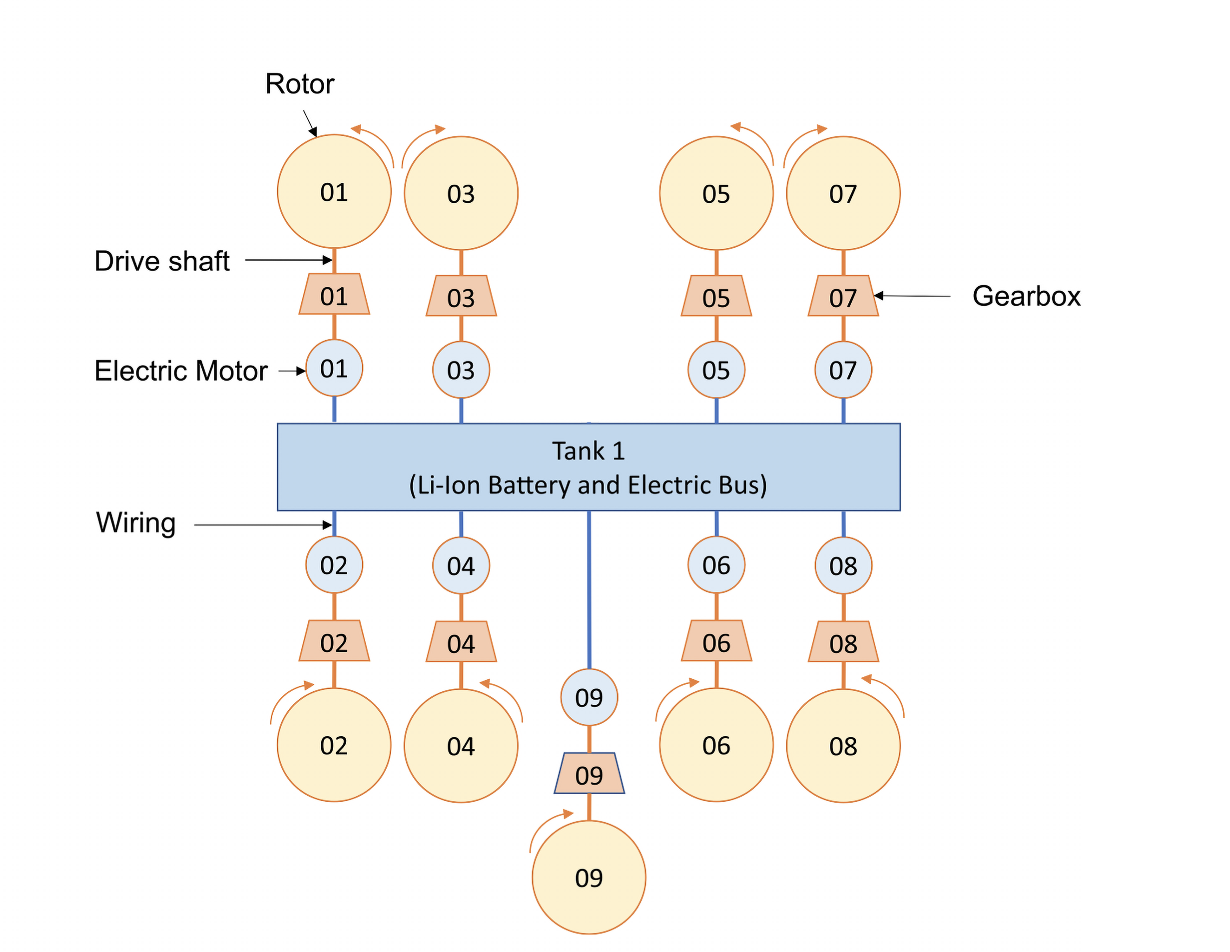
Figure 14: Motor architecture concept, from Ref. [15].

B.1.9 Fuselage Mass

Assumptions and Limitations:

• The provided equations are highly unit sensitive. Use the provided conversion table to transfer metric units into imperial units, insert the imperial units into the models and re-transfer the results from pounds to kilogram.

• The calculation of the fuselage mass is based on statistical mass estimation methods. The structural and geometric properties of the stringers, frames and skins are NOT taken into account. Consideration of the structural calculation may contribute to a significant future extension of the model.

The fuselage mass accounts for the structural mass of the frames, stringer, and skin of the main fuselage.

Raymer:

$$W_{\text{FUS}}=0.052\cdot S_{\text{FUS}}^{0.086}\cdot(n_{z}W_{0})^{0.177}l_{\text{HT}}^{-0.051}\left(\frac{l_{\text{FS}}}{d_{\text{FS}}}\right)^{-0.072}q^{0.241}+11.9\cdot(V_{P}\Delta P)^{0.271}$$ (38)

Nicolai:

$$W_{\text{FUS}}=200\left[\left(\frac{n_{z}W_{0}}{10^{5}}\right)^{0.286}\left(\frac{l_{F}}{10}\right)^{0.857}\left(\frac{w_{F}+d_{F}}{10}\right)\left(\frac{V_{H}}{100}\right)^{0.338}\right]^{1.1}$$ (39)

where:

• $W_{\text{FUS}}$ = predicted weight of the fuselage in lbf.

• $S_{\text{FUS}}$ = fuselage wetted area in ft².

• $l_{\text{FS}}$ = length of fuselage structure (forward bulkhead to aft frame) in ft.

• $d_{\text{FS}}$ = depth of fuselage structure in ft.

• $V_{P}$ = volume of pressurized cabin section in ft³.

• $\Delta P$ = cabin pressure differential, in psi (typically 8 psi).

• $l_{F}$ = fuselage length in ft.

• $w_{F}$ = fuselage max width in ft.

• $d_{F}$ = fuselage max depth in ft.

• $l_{\text{HT}}$ = length of fuselage structure.

• $n_{z}$ = ultimate load factor.

• $W_{0}$ = design gross weight in lbf.

• $q$ = dynamic pressure at cruise.

• $V_{H}$ = maximum level airspeed at sea level (S-L) in knots equivalent airspeed (KEAS).

B.1.10 Systems Mass

Assumptions and Limitations:

• The provided equations are highly unit sensitive. Use the provided conversion table to transfer metric units into imperial units, insert the imperial units into the models and re-transfer the results from pounds to kilogram.

The systems mass accounts for the flight control system and avionics. We assume it also covers air conditioning, lights and other non-flying electronics.

Raymer:

$$M_{system_{R}}=0.053\cdot l_{\text{FS}}^{1.536}\cdot b^{0.371}\cdot\left(n_{z}W_{0}\cdot 10^{-4}\right)^{0.80}$$ (40)

Nicolai:

$$M_{system_{N}}=1.08W_{0}^{0.7}$$ (41)

where:

• $W_{\text{CTRL}}$ = predicted weight of the flight control system in lbf.

• $l_{\text{FS}}$ = length of fuselage structure in ft.

• $b$ = wingspan in ft.

• $n_{z}$ = ultimate load factor.

• $W_{0}$ = design gross weight in lbf.

Resulting in:

$$M_{system}=\frac{M_{system_{R}}+M_{system_{N}}}{2}$$ (42)

B.1.11 Furnishing Mass

Assumptions and Limitations:

• The provided equations are highly unit sensitive. Use the provided conversion table to transfer metric units into imperial units, insert the imperial units into the models and re-transfer the results from pounds to kilogram.

The furnish mass accounts for interior of the eVTOL, like seating and other travel-experience related equipment like entertainment.

Raymer:

$$M_{furn_{R}}=0.0582W_{0}-65$$ (43)

Nicolai:

$$M_{furn_{N}}=34.5N_{\text{CREW}}q_{H}^{0.25}$$ (44)

where:

• $W_{\text{FURN}}$ = predicted weight of furnishings in lbf.

• $W_{0}$ = design gross weight (maximum take-off mass, MTOM) in lbf.

• $N_{\text{CREW}}$ = number of crew.

• $q_{H}$ = dynamic pressure at max level airspeed, in lbf/ft².

Resulting in:

$$M_{furnish}=\frac{M_{furn_{R}}+M_{furn_{N}}}{2}$$ (45)

B.2 Aerodynamic Model

In this model we use a simplified aerodynamic lift and drag model to calculate lift coefficient $C_{L}$ and drag coefficient $C_{D}$ of the eVTOL wing, based on Ref. [8] and Ref. [34]. The airfoil data is taken from Ref. [35] at $Re=200,000$.

B.2.1 Lift Model

Within this framework only the pre-stall aerodynamics are considered. A linear pre-stall lift curve is assumed with a stall angle of attack at 15°. According [34], the finite-wing-lift-curve slope $\alpha_{wing}$ is described by:

$$\alpha_{wing}=\frac{\alpha_{airfoil}}{1+\frac{\alpha_{airfoil}}{\pi\cdot AR\cdot e}}$$ (46)

where $AR$ is the wing aspect ratio, $e$ is the oswald span efficiency, set to 0.8, and $\alpha_{airfoil}$ is the airfoil-lift-curve slope. During the development of this model there are two airfoil profiles in consideration. Based on Ref. [34] and in the interest of simplicity the symmetric NACA 0012 profile (0$\%$ camber, 12$\%$ max thickness at 30$\%$ chord, Ref. [34]) can be used. To simulate an airfoil with camber, the NACA 2412 (can be used as it provides more lift at lower angle of attacks compared to the NACA 0012 (2$\%$ max camber at 40$\%$ chord, 12$\%$ max thickness at 30$\%$ chord, Ref. [34]) making it more efficient in urban and regional air mobility. For detailed airfoil info see Appendix B.2.3. The finite-wing lift coefficient can be written as:

$$C_{L}=\frac{\alpha_{airfoil}}{1+\frac{\alpha_{airfoil}}{\pi\cdot AR\cdot e}}\cdot\alpha+C_{L_{0}}=\alpha_{wing}\cdot\alpha+C_{L_{0}}$$ (47)

where $C_{L_{0}}$ is the lift coefficient at zero angle of attack (equals 0 for NACA 0012) and $\alpha$ is the angle of attack. The slope of the lift coefficient of the airfoil NACA 0012 and NACA 2412 are computed with linear regression using the data from Table 14 and 13 in the Appendix. The airfoils can be described as followed:

$$\text{NACA0012}:C_{L}=5.4225(1/rad)\cdot\alpha(rad)$$ (48)

$$\text{NACA2412}:C_{L}=4.0923(1/rad)\cdot\alpha(rad)+0.415$$ (49)

This results in total lift, where $\rho$ is the air density, $V$ is the aircraft’s true air speed, $S$ is the wings reference area:

$$L=\frac{1}{2}\cdot\rho\cdot V^{2}\cdot S\cdot C_{L}=\frac{1}{2}\cdot\rho\cdot V^{2}\cdot S\cdot\left(\frac{\alpha_{airfoil}}{1+\frac{\alpha_{airfoil}}{\pi\cdot AR\cdot e}}\cdot\alpha+C_{L_{0}}\right)$$ (50)

B.2.2 Drag Model

The model used is based on the lifting line theroy [34] and assumes finite-wing-drag coefficient as composition of induced drag $C_{D_{i}}$ and parasite drag $C_{D_{min}}$:

$$C_{D_{min}}=C_{D_{min}}+C_{D_{i}}$$ (51)

with

$$C_{D_{i}}=\frac{C_{L}^{2}}{\pi\cdot AR\cdot e}$$ (52)

and $C_{D_{min}}=0.0397$ based on the approach by Ref. [6] and the wind-tunnel experiments of Ref.[49], accounting for additional drag of the lifting rotors of a lift+cruise configuration. Resulting in following drag model:

$$C_{D_{min}}=0.0397+\frac{C_{L}^{2}}{\pi\cdot AR\cdot e}$$ (53)

and total drag:

$$D=\frac{1}{2}\cdot\rho\cdot V^{2}\cdot S\cdot C_{D}=\frac{1}{2}\cdot\rho\cdot V^{2}\cdot S\cdot\left(0.0397+\frac{C_{L}^{2}}{\pi\cdot AR\cdot e}\right)$$ (54)

The resulting lift and drag coefficient models are shown in Fig. 15. Within the model, a constant angle of attack during climb $\alpha_{climb}=8$° and $\alpha_{climb}=3$° (subject to change).

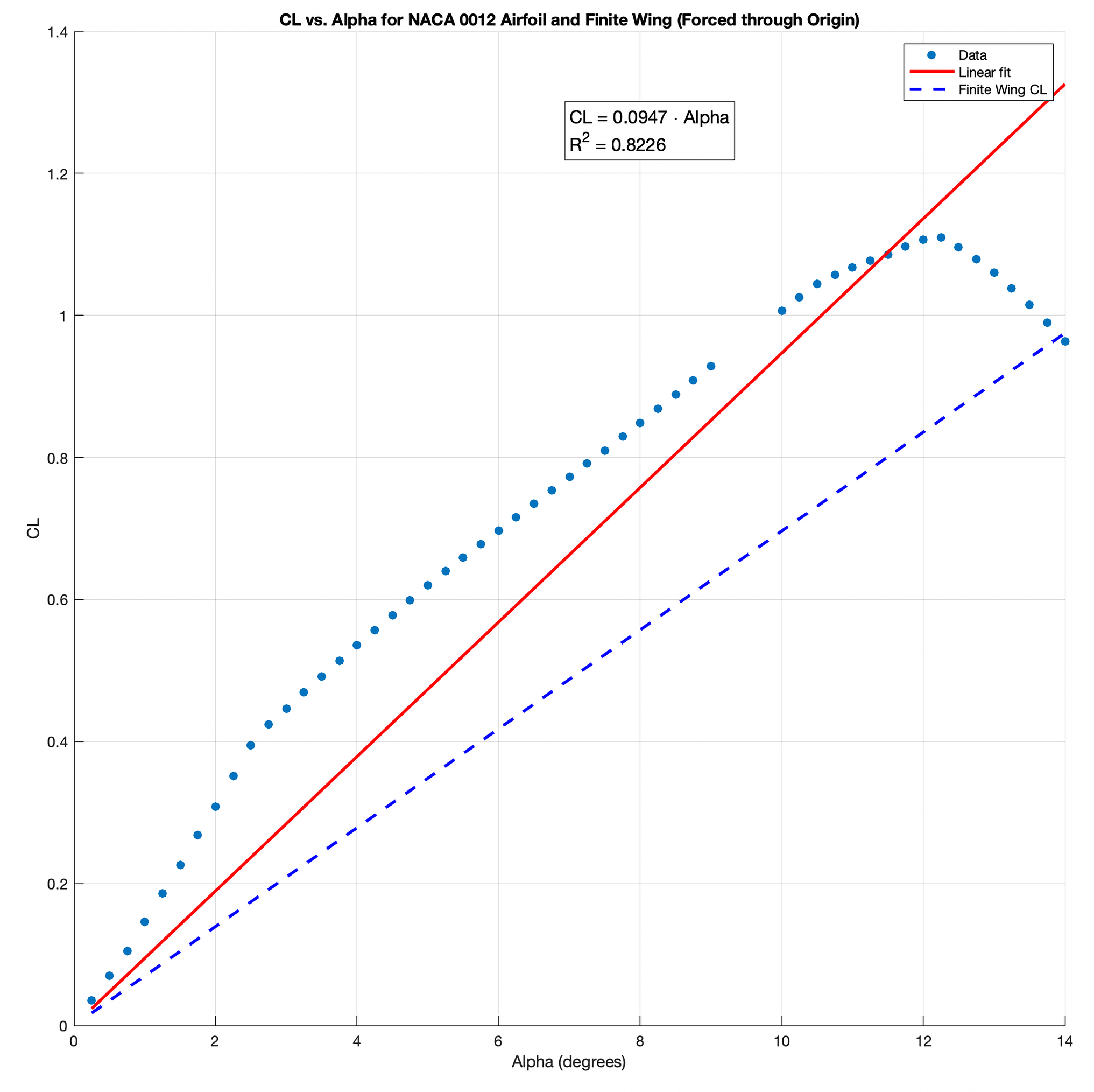
(a) Lift coefficient model for NACA0012.

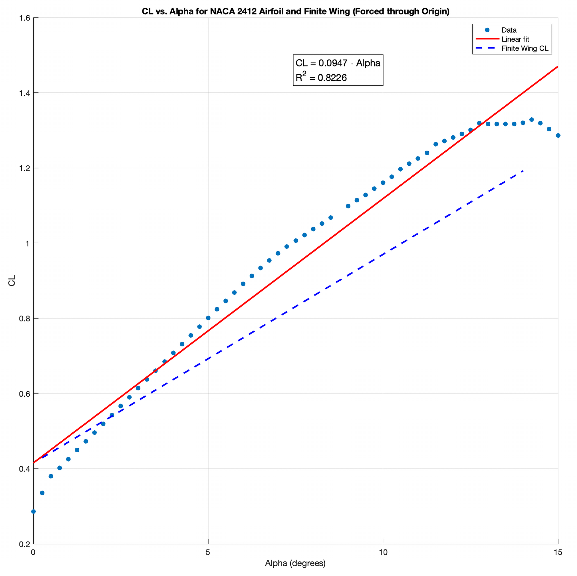
(b) Lift coefficient model for NACA2412.

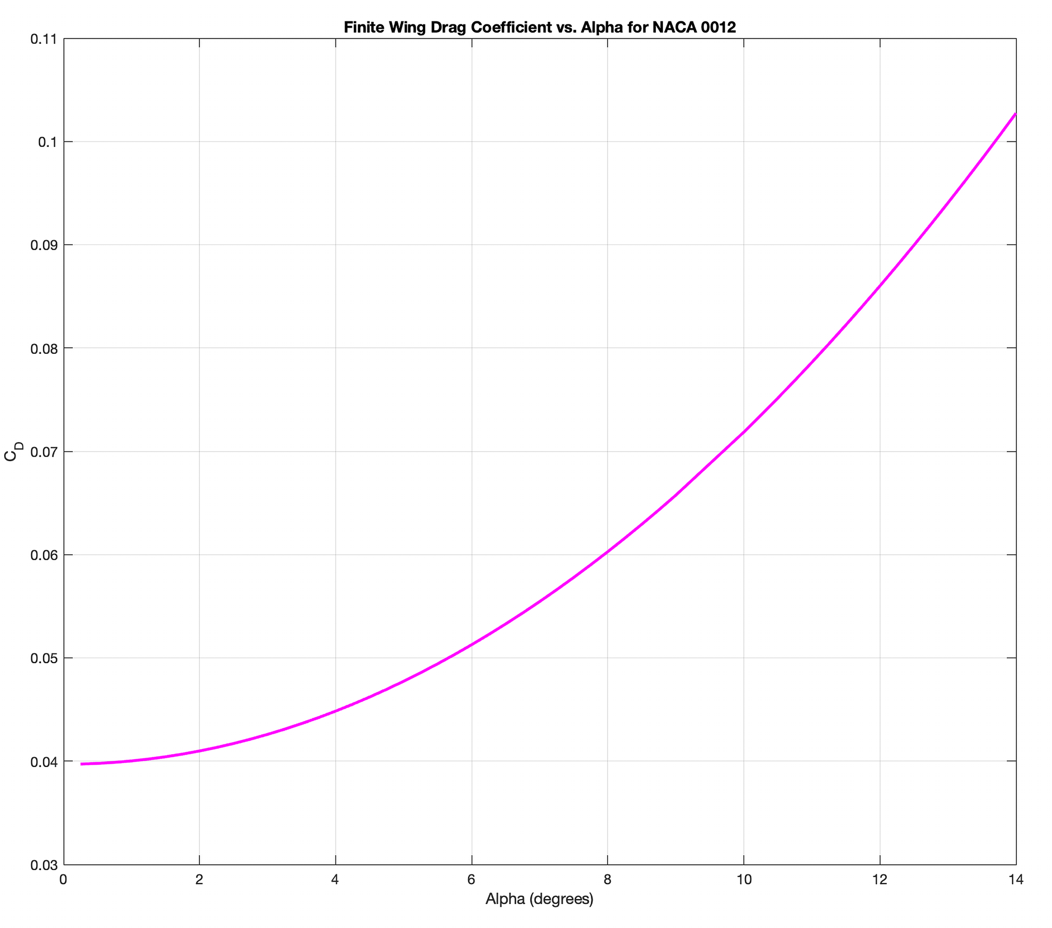
(c) Drag coefficient model for NACA0012.

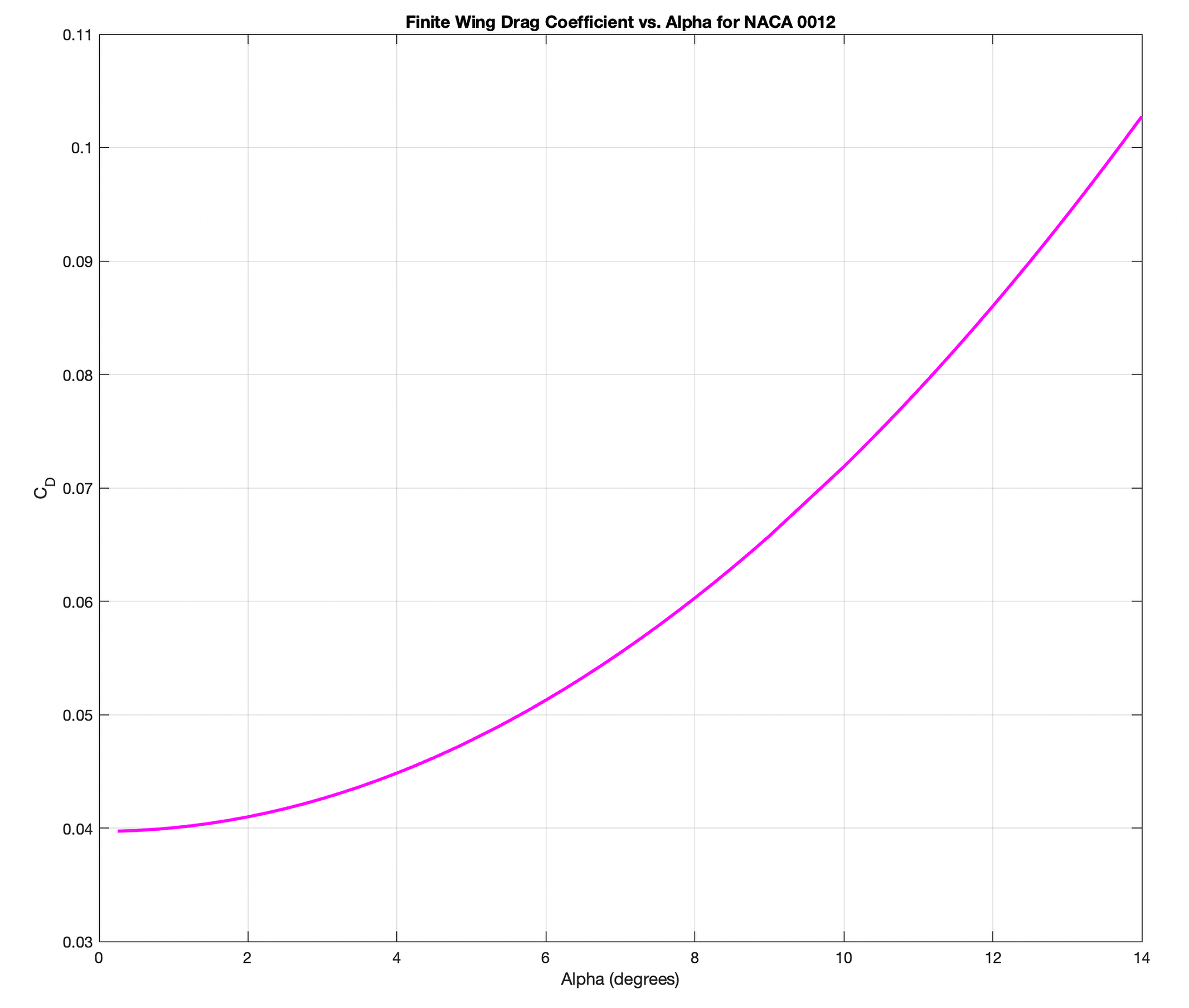
(d) Drag coefficient model for NACA2412.

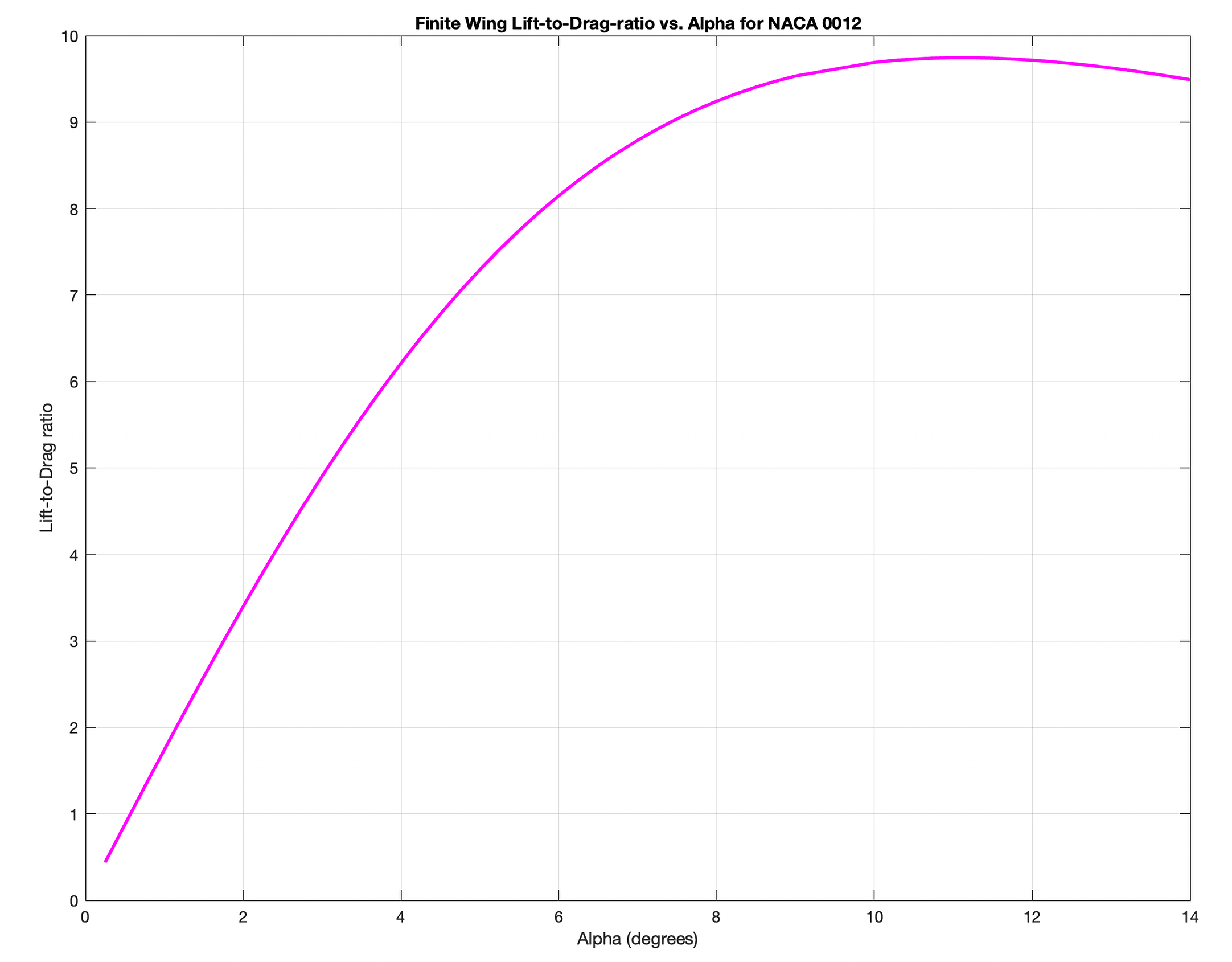
(e) Lift-to-drag ratio model for NACA0012.

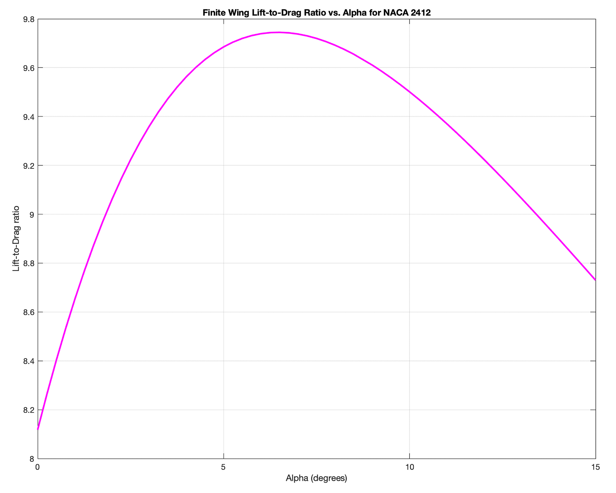
(f) Lift-to-drag ratio model for NACA2412.

Figure 15: Airfoils regression models.

B.2.3 Airfoil Data

NACA 2412 Data according [35].

$\alpha$	$C_{L}$	$C_{D}$	$C_{Dp}$	$C_{M}$	Top_Xtr	Bot_Xtr
0.000	0.2860	0.01001	0.00485	-0.0608	0.8392	0.9789
0.250	0.3359	0.00994	0.00469	-0.0650	0.8247	0.9917
0.500	0.3796	0.00985	0.00451	-0.0682	0.8082	1.0000
0.750	0.4025	0.00981	0.00436	-0.0672	0.7901	1.0000
1.000	0.4257	0.00980	0.00424	-0.0662	0.7719	1.0000
1.250	0.4491	0.00982	0.00415	-0.0652	0.7537	1.0000
1.500	0.4727	0.00988	0.00410	-0.0642	0.7356	1.0000
1.750	0.4959	0.00996	0.00409	-0.0631	0.7163	1.0000
2.000	0.5193	0.01005	0.00410	-0.0621	0.6973	1.0000
2.250	0.5428	0.01017	0.00413	-0.0611	0.6786	1.0000
2.500	0.5663	0.01030	0.00417	-0.0601	0.6604	1.0000
2.750	0.5899	0.01045	0.00424	-0.0592	0.6427	1.0000
3.000	0.6136	0.01062	0.00432	-0.0582	0.6255	1.0000
3.250	0.6373	0.01080	0.00443	-0.0572	0.6088	1.0000
3.500	0.6610	0.01099	0.00456	-0.0563	0.5924	1.0000
3.750	0.6847	0.01119	0.00470	-0.0554	0.5757	1.0000
4.000	0.7080	0.01141	0.00483	-0.0543	0.5577	1.0000
4.250	0.7311	0.01161	0.00498	-0.0533	0.5375	1.0000
4.500	0.7543	0.01182	0.00515	-0.0522	0.5178	1.0000
4.750	0.7778	0.01205	0.00534	-0.0513	0.4995	1.0000
5.000	0.8010	0.01229	0.00554	-0.0503	0.4800	1.0000
5.250	0.8238	0.01256	0.00572	-0.0493	0.4589	1.0000
5.500	0.8465	0.01279	0.00593	-0.0482	0.4349	1.0000
5.750	0.8687	0.01309	0.00616	-0.0471	0.4112	1.0000
6.000	0.8911	0.01338	0.00642	-0.0461	0.3854	1.0000
6.250	0.9129	0.01373	0.00670	-0.0450	0.3582	1.0000
6.500	0.9339	0.01415	0.00702	-0.0438	0.3278	1.0000
6.750	0.9541	0.01465	0.00740	-0.0425	0.2937	1.0000
7.000	0.9731	0.01526	0.00785	-0.0411	0.2573	1.0000
7.250	0.9908	0.01600	0.00841	-0.0396	0.2186	1.0000
7.500	1.0067	0.01693	0.00909	-0.0378	0.1782	1.0000
7.750	1.0218	0.01795	0.00991	-0.0360	0.1446	1.0000
8.000	1.0370	0.01896	0.01076	-0.0341	0.1225	1.0000
8.250	1.0523	0.01995	0.01166	-0.0323	0.1086	1.0000
8.500	1.0679	0.02091	0.01261	-0.0305	0.0995	1.0000
9.000	1.0982	0.02292	0.01462	-0.0268	0.0875	1.0000
9.250	1.1137	0.02387	0.01556	-0.0251	0.0830	1.0000
9.500	1.1282	0.02523	0.01687	-0.0234	0.0794	1.0000
9.750	1.1448	0.02608	0.01784	-0.0218	0.0764	1.0000
10.000	1.1606	0.02701	0.01883	-0.0201	0.0733	1.0000
10.250	1.1764	0.02814	0.01993	-0.0187	0.0705	1.0000
10.500	1.1960	0.02971	0.02152	-0.0179	0.0678	1.0000
10.750	1.2108	0.03066	0.02263	-0.0162	0.0656	1.0000
11.000	1.2253	0.03171	0.02378	-0.0146	0.0632	1.0000
11.250	1.2401	0.03283	0.02494	-0.0132	0.0610	1.0000
11.500	1.2632	0.03501	0.02707	-0.0133	0.0582	1.0000
11.750	1.2711	0.03605	0.02834	-0.0109	0.0568	1.0000
12.000	1.2809	0.03736	0.02983	-0.0090	0.0549	1.0000
12.250	1.2900	0.03870	0.03129	-0.0072	0.0530	1.0000
12.500	1.3004	0.04002	0.03266	-0.0058	0.0513	1.0000
12.750	1.3189	0.04267	0.03530	-0.0055	0.0491	1.0000
13.000	1.3172	0.04432	0.03723	-0.0029	0.0482	1.0000
13.250	1.3163	0.04631	0.03947	-0.0008	0.0469	1.0000
13.500	1.3164	0.04839	0.04175	0.0008	0.0456	1.0000
13.750	1.3172	0.05044	0.04393	0.0021	0.0443	1.0000
14.000	1.3198	0.05245	0.04601	0.0031	0.0432	1.0000
14.250	1.3283	0.05480	0.04836	0.0038	0.0419	1.0000
14.500	1.3192	0.05878	0.05258	0.0048	0.0411	1.0000
14.750	1.3035	0.06249	0.05658	0.0053	0.0407	1.0000
15.000	1.2862	0.06682	0.06119	0.0051	0.0403	1.0000

Table 13: XFOIL Calculated Polar for NACA 2412 Airfoil

NACA 0012 Data according [35].

$\alpha$	$C_{L}$	$C_{D}$	$C_{Dp}$	$C_{M}$	Top_Xtr	Bot_Xtr
0.000	0.0000	0.01020	0.00520	0.0000	0.9046	0.9047
0.250	0.0350	0.01022	0.00521	-0.0004	0.8886	0.9182
0.500	0.0700	0.01025	0.00522	-0.0009	0.8696	0.9304
0.750	0.1048	0.01028	0.00521	-0.0015	0.8482	0.9424
1.000	0.1454	0.01034	0.00519	-0.0033	0.8255	0.9510
1.250	0.1861	0.01040	0.00518	-0.0054	0.7978	0.9593
1.500	0.2255	0.01048	0.00517	-0.0072	0.7684	0.9686
1.750	0.2684	0.01056	0.00512	-0.0100	0.7357	0.9756
2.000	0.3085	0.01066	0.00509	-0.0122	0.7012	0.9843
2.250	0.3513	0.01075	0.00504	-0.0152	0.6637	0.9915
2.500	0.3942	0.01085	0.00497	-0.0183	0.6249	0.9979
2.750	0.4235	0.01094	0.00492	-0.0188	0.5886	1.0000
3.000	0.4462	0.01104	0.00489	-0.0180	0.5545	1.0000
3.250	0.4689	0.01118	0.00489	-0.0172	0.5202	1.0000
3.500	0.4915	0.01134	0.00492	-0.0163	0.4857	1.0000
3.750	0.5138	0.01153	0.00498	-0.0155	0.4509	1.0000
4.000	0.5357	0.01176	0.00507	-0.0145	0.4160	1.0000
4.250	0.5571	0.01203	0.00521	-0.0134	0.3810	1.0000
4.500	0.5782	0.01234	0.00536	-0.0123	0.3456	1.0000
4.750	0.5990	0.01268	0.00556	-0.0111	0.3101	1.0000
5.000	0.6195	0.01306	0.00580	-0.0099	0.2744	1.0000
5.250	0.6395	0.01350	0.00609	-0.0086	0.2398	1.0000
5.500	0.6591	0.01400	0.00643	-0.0072	0.2077	1.0000
5.750	0.6784	0.01455	0.00683	-0.0058	0.1796	1.0000
6.000	0.6971	0.01516	0.00729	-0.0043	0.1563	1.0000
6.250	0.7161	0.01577	0.00781	-0.0028	0.1374	1.0000
6.500	0.7351	0.01641	0.00837	-0.0013	0.1223	1.0000
6.750	0.7535	0.01712	0.00900	0.0003	0.1104	1.0000
7.000	0.7725	0.01776	0.00961	0.0018	0.1005	1.0000
7.250	0.7919	0.01844	0.01031	0.0033	0.0925	1.0000
7.500	0.8096	0.01936	0.01114	0.0049	0.0858	1.0000
7.750	0.8300	0.01995	0.01181	0.0062	0.0799	1.0000
8.000	0.8481	0.02112	0.01285	0.0077	0.0749	1.0000
8.250	0.8690	0.02173	0.01362	0.0089	0.0707	1.0000
8.500	0.8890	0.02251	0.01438	0.0101	0.0667	1.0000
8.750	0.9087	0.02387	0.01574	0.0112	0.0635	1.0000
9.000	0.9291	0.02472	0.01674	0.0124	0.0604	1.0000
10.000	1.0067	0.02966	0.02206	0.0168	0.0511	1.0000
10.250	1.0251	0.03077	0.02323	0.0179	0.0492	1.0000
10.500	1.0445	0.03262	0.02503	0.0185	0.0474	1.0000
10.750	1.0571	0.03445	0.02718	0.0203	0.0462	1.0000
11.000	1.0681	0.03636	0.02942	0.0222	0.0451	1.0000
11.250	1.0773	0.03842	0.03177	0.0241	0.0441	1.0000
11.500	1.0860	0.04035	0.03390	0.0258	0.0430	1.0000
11.750	1.0969	0.04194	0.03558	0.0272	0.0419	1.0000
12.000	1.1068	0.04366	0.03735	0.0286	0.0410	1.0000
12.250	1.1101	0.04727	0.04108	0.0298	0.0401	1.0000
12.500	1.0959	0.04960	0.04372	0.0334	0.0399	1.0000
12.750	1.0790	0.05258	0.04700	0.0360	0.0397	1.0000
13.000	1.0599	0.05626	0.05095	0.0372	0.0396	1.0000
13.250	1.0385	0.06069	0.05564	0.0369	0.0396	1.0000
13.500	1.0150	0.06603	0.06120	0.0352	0.0396	1.0000
13.750	0.9898	0.07237	0.06774	0.0319	0.0398	1.0000
14.000	0.9632	0.07976	0.07532	0.0275	0.0399	1.0000

Table 14: XFOIL Calculated Polar for NACA 0012 Airfoil

B.3 Power & Energy Model

B.3.1 Aircraft Efficiencies

Assumptions and Limitations:

• The provided framework assumes fix system efficiencies. These can be changed as required for customized simulations.

Item	Symbol	Value	Source
Electric Efficiency	$\eta_{e}$	0.9	[13]
Hover Propulsive Efficiency	$\eta_{hp}$	0.7	[16]
Propulsive Efficiency	$\eta_{p}$	0.85	[13]
Hover System Efficiency	$\eta_{h}=\eta_{e}\cdot\eta_{hp}$	0.63	[16]
Overall System Efficiency	$\eta_{c}=\eta_{p}\cdot\eta_{e}$	0.77	[16]

Table 15: System efficiencies.

B.3.2 Momentum Theory Power Model

Assumptions and Limitations:

• The power modelling within the provided framework is based on propeller momentum theory, using flight equilibrium relationships in hover, climb and cruise flight. For improved rotor dynamics accuracy, one should enhance this model using Blade Element Momentum Theory.

• Steady, unaccelerated flight (forces equilibrium) in each flight phase is assumed.

• For simulation, number of propeller in climb/cruise configuration is assumed to be 1. The number of vertical lift propeller is assumed to be 8.

B.3.3 Hover Power Required:

Power requirements in hover flight account for steady hover, where thrust and aircraft mass are balanced and power is needed to overcome propeller induced velocity, as illustrated in Fig. (16):

$$T_{required_{hover}}=MTOM\cdot g$$ (55)

resulting in a power requirement of:

$$P_{required_{hover}}=\frac{T_{total}\cdot v_{i}}{\eta_{h}}=\frac{MTOM\cdot g}{\eta_{h}}\cdot\sqrt{\frac{\sigma}{2\cdot\rho}}$$ (56)

• $v_{i}$ ($m/s^{2}$) = propeller induced velocity, defined by:

$$v_{i}=\sqrt{\frac{\sigma}{2\cdot\rho}}$$ (57)

• $\rho$ ($kg/m^{2}$) = air density in hover.

• $\sigma$ ($N/m^{2}$) = propeller disk loading, defined by:

$$\sigma=\frac{T_{prop}}{A_{prop}}=\frac{T_{prop}}{\pi\cdot R_{prop}^{2}}$$ (58)

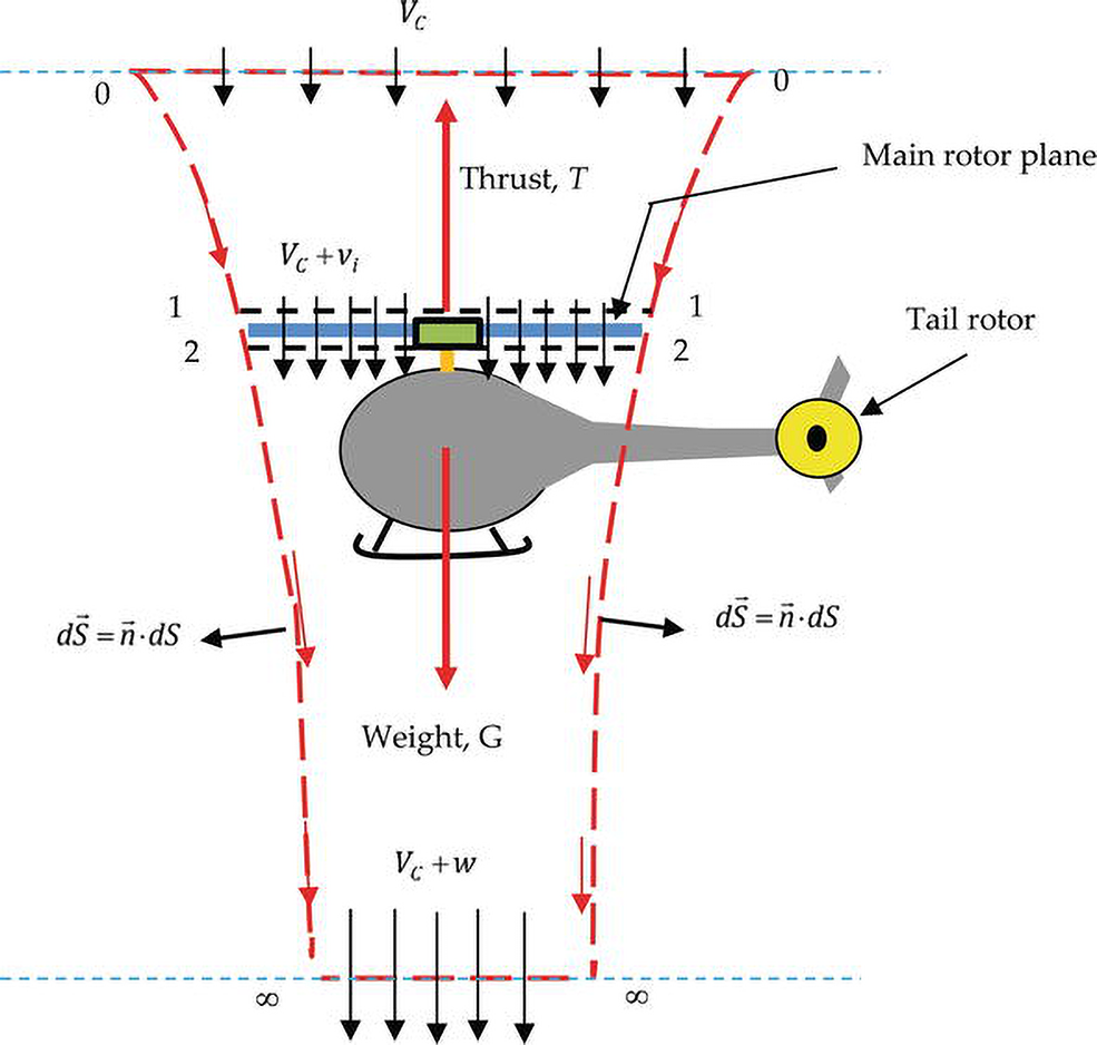
Figure 16: Forces in Hover, from Ref. [50].

B.3.4 Climb Power Required:

Power required in climb is defined by:

$$P_{climb}=P_{req_{flight}}+P_{ind_{prop}}=\frac{T_{req_{climb}}\cdot V_{climb}}{\eta_{c}}+\frac{T_{prop_{climb}}\cdot v_{i}}{\eta_{c}}\cdot n_{prop}$$ (59)

• $P_{req_{flight}}$ (W) = power required to maintain flight, defined by:

$$P_{req_{flight}}=\frac{T_{req_{climb}}\cdot V_{climb}}{\eta_{c}}$$ (60)

• $T_{req_{climb}}$ (N) = thrust required in climb, illustrated in Fig. (17) and defined by:

$$T_{required_{climb}}=D_{climb}+MTOM\cdot sin(\theta)$$ (61)

• $D_{climb}$ (N) = aircraft drag in climb flight (eq. (54)), using $V_{climb}$ (eq. (65)) and $\alpha_{climb}$.

• MTOM (kg) = max. take-off mass (eq. (24)).

• $\theta$ (°) = climb angle, assumed to be equal to angle of attack in climb $\alpha_{climb}$.

• $P_{ind_{porp}}$ (W) = propeller induced power required, defined by:

$$P_{ind_{prop}}=\frac{T_{prop_{climb}}\cdot v_{i}}{\eta_{c}}\cdot n_{prop}$$ (62)

• $T_{prop_{climb}}$ (N) = $T_{req_{climb}}/n_{prop}$ = thrust required per propeller.

• $n_{prop}$ (-) = number of propeller.

• $v_{i}$ (m/s) = propeller induced velocity, defined by equation (57

The horizontal speed during climb phase (Climb Speed), accounting for climb angle $\theta=\alpha_{climb}$, assuming zero wind, is defined by:

$$\text{Climb Condition: }MTOM\cdot g\cdot cos(\theta)=L=\frac{1}{2}\cdot\rho\cdot V_{climb}^{2}\cdot S\cdot C_{L_{climb}}$$ (63)

Resulting in the trivial conditions during climb flight:

$$\text{Mass Condition: }MTOM=\frac{1}{2\cdot g\cdot cos(\theta)}\cdot\rho\cdot V_{climb}^{2}\cdot S\cdot C_{L_{climb}}$$ (64)

and,

$$\text{Climb Speed Condition: }V_{climb}=\sqrt{\frac{2\cdot MTOM\cdot g\cdot cos(\theta)}{\rho\cdot S\cdot C_{L_{climb}}}}$$ (65)

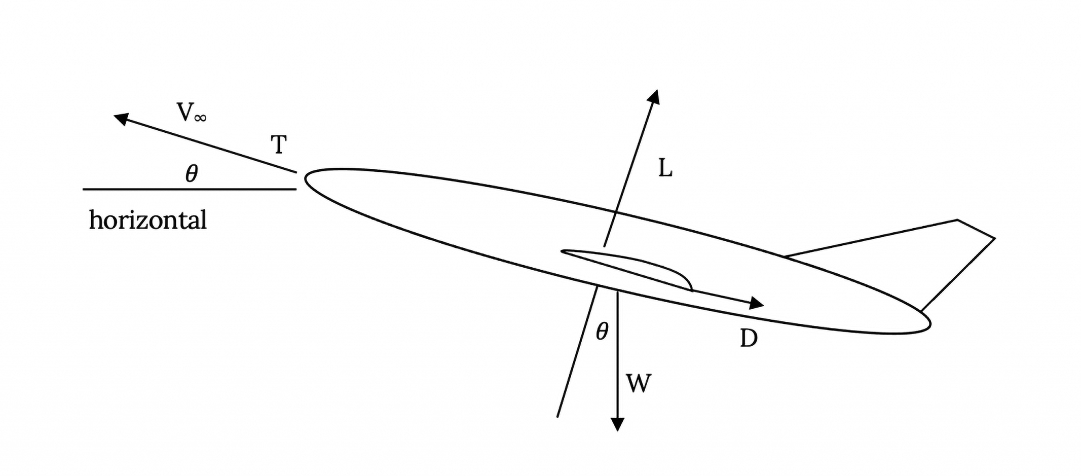
Figure 17: Forces in Climb, from Ref. [51].

B.3.5 Cruise Power Required:

Power required to maintain steady cruise flight is similar derived as cruise power, defined by:

$$P_{cruise}=P_{req_{flight}}+P_{ind_{prop}}=\frac{T_{req_{cruise}}\cdot V_{cruise}}{\eta_{c}}+\frac{T_{prop_{cruise}}\cdot v_{i}}{\eta_{c}}\cdot n_{prop}$$ (66)

• $T_{req_{cruise}}$ (N) = thrust required in cruise, illustrated in Fig. (18) and defined by:

$$T_{required_{cruise}}=D_{cruise}$$ (67)

• $D_{climb}$ (N) = aircraft drag in cruise flight (eq. (54)), using $V_{cruise}$ (eq. (70))

During horizontal, unaccelerated flight, the cruise speed is defined by:

$$\text{Cruise Condition: }MTOM\cdot g=L=\frac{1}{2}\cdot\rho\cdot V_{cruise}^{2}\cdot S\cdot C_{L_{cruise}}$$ (68)

Resulting in the trivial conditions during cruise flight:

$$\text{Mass Condition: }MTOM=\frac{1}{2\cdot g}\cdot\rho\cdot V_{cruise}^{2}\cdot S\cdot C_{L_{cruise}}$$ (69)

and,

$$\text{Cruise Speed Condition: }V_{cruise}=\sqrt{\frac{2\cdot MTOM\cdot g}{\rho\cdot S\cdot C_{L_{cruise}}}}$$ (70)

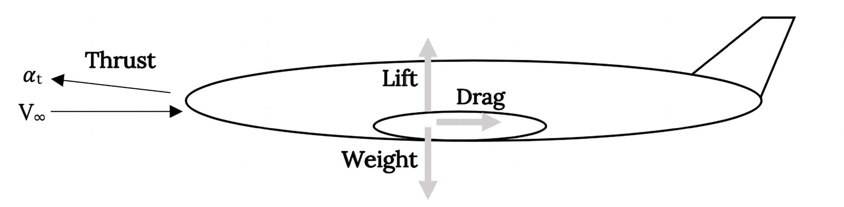
Figure 18: Static Force Balance in Straight and Level Flight, from Ref. [51].

B.3.6 Energy Requirements

The required energy (Wh) in each flight phase can be computed using the relationship:

$$E_{i}=\sum_{i}\text{P}_{i}\cdot t_{i}$$ (71)

The specific battery energy can be calculated when dividing the energy by battery mass:

$$e_{i}=\frac{E_{i}}{M_{bat}}$$ (72)

• $M_{bat}$ (kg) = battery mass, defined by eq. (25), with:

$$E_{useable}=E_{trip}+E_{reserve}$$ (73)

• $E_{trip}$ (Wh) = sum of energy required in hover, climb and cruise, using eq. (71).

• $E_{reserve}$ (Wh) = energy required in reserve flight, accounting for 30 min for VFR and 45min for IFR flight with cruise power according FAA.

Within this model the end-of-life battery status is considered, which is set to 80% of BOL (begin-of-life) capacity:

$$e_{BAT_{EOL}}=0.8\cdot\rho_{bat}$$ (74)

The battery ceiling is set as 90% SOC and the floor as 10% SOC, making these portions unusable for trips [16]. Resulting in usable specific energy:

$$e_{\text{usable}}=0.8\cdot e_{BAT_{EOL}}=0.64\cdot\rho_{bat}=e_{trip_{design}}+e_{reserve}$$ (75)

or expressed as the battery specific energy budget for the trip:

$$e_{trip_{design}}=0.64\cdot\rho_{bat}-e_{reserve}$$ (76)

or

$$e_{trip}\leq 0.64\cdot\rho_{bat}-e_{reserve}$$ (77)

$$1.5623\cdot(e_{trip}+e_{reserve})\leq\rho_{bat}$$ (78)

Resulting in total battery energy storage capacity of:

$$E_{Bat_{total}}=\rho_{bat}\cdot M_{bat}$$ (79)

B.4 Economic Model

B.4.1 Operations Model

• The eVTOL operates within a daily operation window, defined by a fixed value of $T_{D}$ (hours).

• Within this operation window the eVTOL can perform flights, characterized by travel time $t_{trip}$ and battery depth-of-discharge (DOD), defined in Appednix B.5.

• The time between each flight is defined as the turnaround-time $T_{T}$. This time accounts for battery recharging as well as passenger/freight swap, but within the model only battery recharging is considered.

• Time for battery recharge is defined by the charging rate $C_{rate_{charge}}$, defined in Appendix B.5.

$$T_{T}=\frac{1}{C_{rate_{charge}}}\cdot DoD=\frac{1}{C_{rate_{charge}}}\cdot\frac{E_{trip}}{E_{Battery}}$$ (80)

with:

$$DoD=\frac{E_{trip}}{E_{Battery}}$$ (81)

The Total Cycle Time Factor (CT), measures the efficiency of transportation operations. It reflects the ratio of non-productive turnaround time to productive trip time, with the "+1" accounting for the complete cycle. A lower value indicates higher operational efficiency by minimizing turnaround time relative to trip time. It is defined by:

$$CT=\frac{T_{T}}{t_{trip}}+1$$ (82)

Fig. (19) depicts an operational framework for eVTOL vehicles, based on Uber Elevate requirements, Ref. [23]. It includes:

• Annual Operation Days ($n_{wd}$): 260 days/year.

• Daily Operation Window ($T_{D}$): 8 hours/day.

• Turnaround Time ($T_{T}$): Function of C-rate and Depth of Discharge (DoD).

• Trip Time ($T_{trip}$): Depends on vehicle speed (V), trip distance ($D_{trip}$), and hover time ($t_{hover}$).

The framework calculates the number of flight cycles and total flight hours within these constraints. Operational parameters like annual-trip-time ratio, annual flight hours, daily flight hours and flight cycles are defined below:

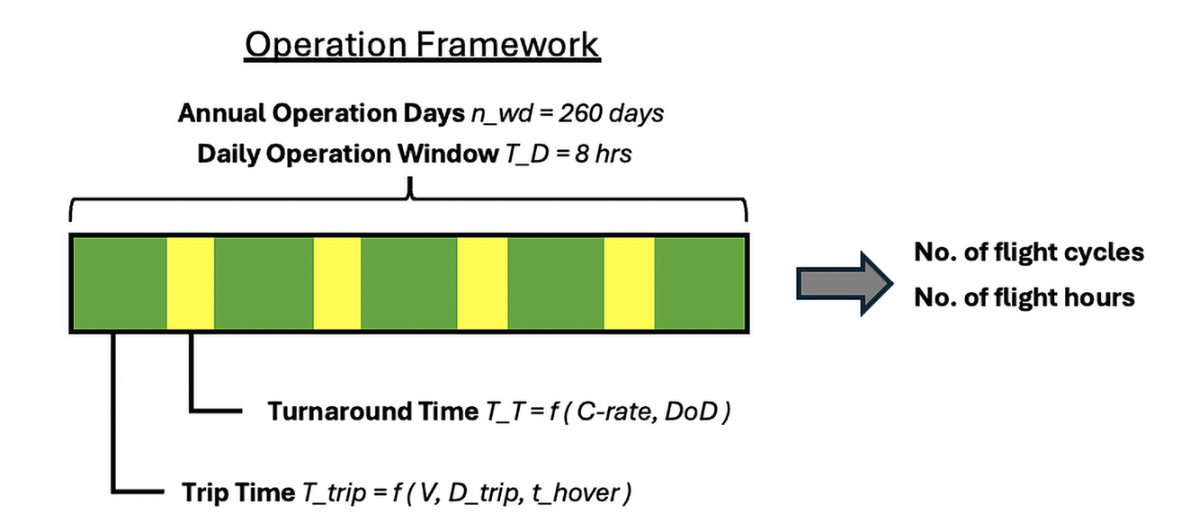
Figure 19: Operations Window.

• $\lambda_{trip}$ = annual-trip-time ratio, defined by equation 83 and 88:

$$\lambda_{trip}=\frac{t_{trip}}{FH_{annual}}$$ (83)

• $FH_{annual}$ (hours) = annual operating flight hours of one eVTOL, defined by equation 84 and 87:

$$FH_{annual}=t_{trip}\cdot FC_{annual}=t_{trip}\cdot n_{WD}\cdot FC_{day}$$ (84)

• $FC_{annual}$ (-) = annual operating flight cycles of one eVTOL, defined by:

$$FC_{annual}=n_{WD}\cdot FC_{day}=n_{WD}\cdot\frac{T_{D}}{t_{trip}\cdot CT}$$ (85)

• $n_{WD}$ (-) = number of operating days per year, set to 260, Ref. [16].

• $FC_{day}$ (-) = daily operating flight cycles of one eVTOL, defined by:

$$FC_{day}=\frac{T_{D}}{t_{trip}\cdot CT}$$ (86)

$$FH_{annual}=n_{WD}\cdot\frac{T_{D}}{CT}$$ (87)

and

$$\lambda_{trip}=\frac{1}{FC_{annual}}=\frac{t_{trip}\cdot CT}{n_{WD}\cdot T_{D}}$$ (88)

B.4.2 Operational Cost Model

Assumptions and Limitations:

• The total operating cost model is structured according the ATA-67 Formula for Direct Operating cost, Ref. [52].

• The sub-assumptions are based on highly variable operational assumptions in real world applications, which can be adjusted depending on the operational business.

B.4.3 Total Operating Cost

The total operating costs of an aircraft per trip are divided into Cash Operating Cost (COC), Cost of Ownership (COO) and Indirect Operating Cost (IOC), according Ref. [52]:

$$TOC=COC+COO+IOC$$ (89)

Each cost element is further subdivided into its components, as shown in Figure 20, in order to obtain as detailed a picture as possible of the cost structure of an eVTOL. The cost calculation is based on the fact that the flight hour is the only value-adding activity of an operator. Therefore, all costs associated with flight operations must be allocated to the flight hour. The sum of COC and COO is also regarded as Direct Operating Cost (DOC), similar to variable costs, and IOC as fixed costs.

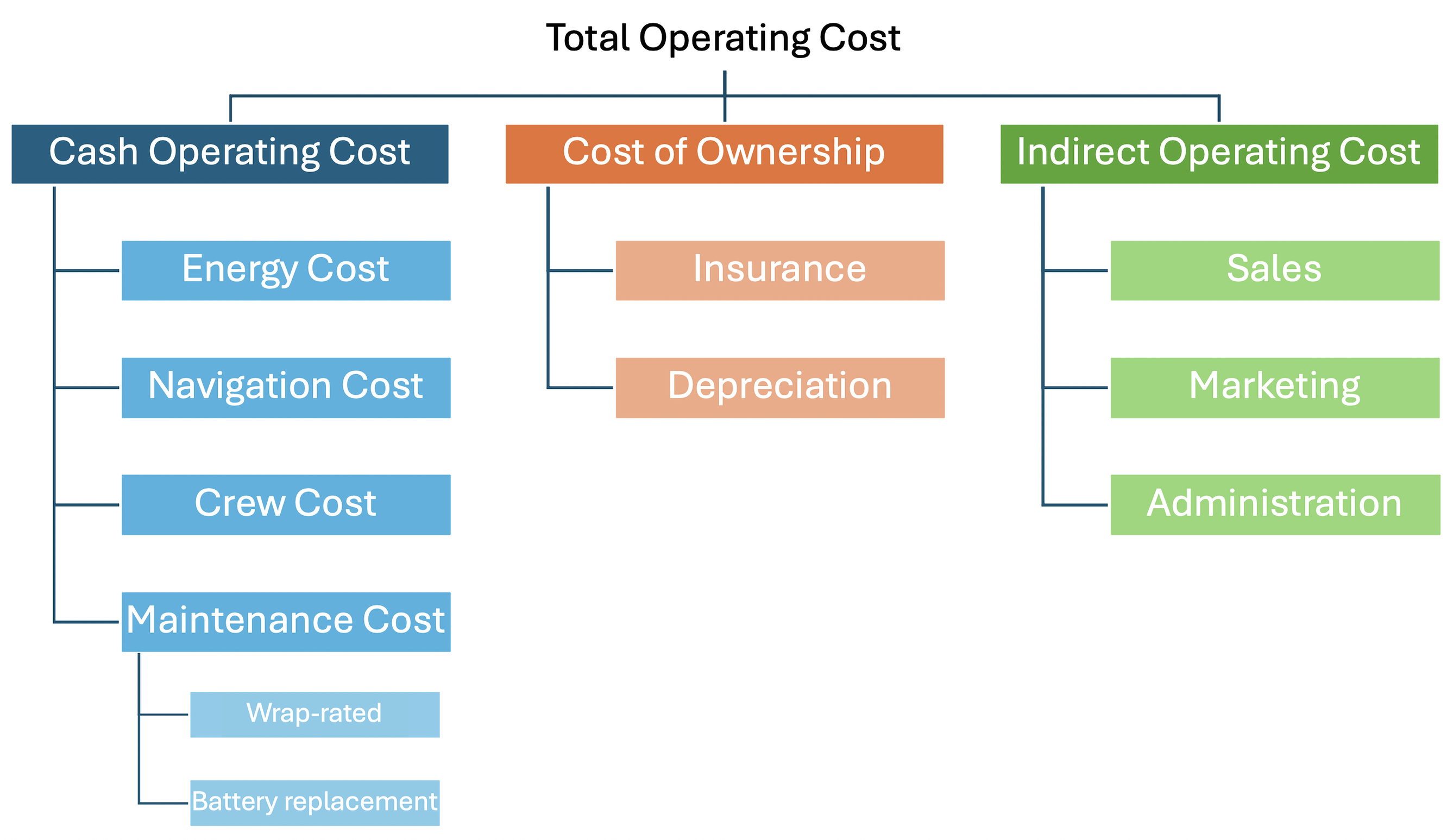
Figure 20: Total operating cost structure.

B.4.4 Cash Operating Cost

Cash operating costs in aviation, akin to variable costs, encompass immediate, out-of-pocket expenses. In this model, they are considered on a trip base and include energy cost $C_{E}$, maintenance cost $C_{M}$, crew cost $C_{C}$, and navigation cost $C_{N}$:

$$COO=C_{E}+C_{M}+C_{C}+C_{N}$$ (90)

Energy Cost

Assumptions and Limitations:

• The framework assumes the energy price and electricity $CO_{2}$ emissions of Germany, accounting 0.096 €/kWh and 0.3784 kg-$CO_{2}$/kWh respectively.

• A dataset for energy prices and $CO_{2}$ emissions is provided on the authors GitHub and can be used for geographic specific analysis.

Energy cost, comparable to fuel cost of combustion-engine aircraft, are defined by the simple relationship:

$$C_{E}=E_{trip}\cdot P_{energy}$$ (91)

with trip energy $E_{trip}$ (kWh) and current energy price $P_{energy}$ (€/kWh). $E_{trip}$ is the used energy amount of the trip flown, and is direct related to power requirements in each flight phase and flight time, thus to mission profile design (velocity, altitude etc.). It is considered, that $P_{energy}$ can vary depending on procedures for generation of electricity, differing in geographical regions, countries and energy policy.

Maintenance Cost

Assumptions and Limitations:

• The computation of this model is based on several static operational assumptions that can significantly influence the potential result.

• $t_{trip}$ in this section is considered in hours.

The maintenance costs, $C_{M}$, are defined by:

$$C_{M}=C_{M_{WR}}+C_{M_{B}}$$ (92)

with $C_{M_{WR}}$ are the wrap-rated maintenance costs:

$$C_{M_{WR}}=MF\cdot MWR\cdot t_{trip}=0.6\cdot 55\cdot t_{trip}=33\cdot t_{trip}$$ (93)

• MF (-) = maintenance man-hours per flight hour ratio, assumed as 0.6, Ref. [13].

• MWR (€/hr) = maintenance wrap-rate, assumed fix at 55€, Ref. [13].

• $t_{trip}$ (hr) = trip duration of the considered flight.

$C_{M_{B}}$ is considered as battery replacement cost, defined by:

$$C_{M_{B}}=n_{Bat}\cdot P_{Bat_{s}}\cdot E_{BAT_{total}}\cdot\lambda_{trip}$$ (94)

• $E_{BAT_{total}}$ (kWh) = total energy storage capacity of the eVTOL-installed battery, defined by eq. (79) in chapter B.3.6.

• $P_{bat_{s}}$ (€/kWh) = energy specific battery acquisition cost. According to [19], the Tesla Model S battery cost was estimated at 155 €/kWh in 2020 and 55 €/kWh in 2030, with current costs ranging from 108 €/kWh to 142 €/kWh. Future eVTOL batteries will likely have higher capacities, requiring special attention, as battery costs can significantly impact the total cost.

Assumptions and Limitations:

• The following trivial assumption applies: Travelling a design trip distance corresponds to discharging one battery charge. In other words, the battery of the eVTOL is designed in such a way that it is sufficient to cover the design trip distance, after which it must be recharged to cover the same distance again. The discharge in the design trip distance does not mean a complete battery discharge, as unusable energy and reserves are also taken into account.

• It is assumed that the reserve is not used, but is considered as energy reserve in battery design.

• When considering the cycle life of the battery, it is assumed that the eVTOL flies the design distance on every flight.

• $n_{Bat}$ (-) = number of required batteries per year. This is highly dependent on the specific battery characteristics and discharge rates. A model for battery cycle-life is proposed and derived in the following:

$$n_{Bat}=\frac{CC_{req_{eVTOL}}}{N_{cycles}}$$ (95)

• $CC_{req_{eVTOL}}$ (-) = annually required charging cycles of the eVTOL, defined by:

$$CC_{req}=\frac{FC_{annual}}{FC_{Bat}}=n_{WD}\cdot\frac{T_{D}}{t_{trip}\cdot DH}\cdot\frac{SE_{trip}}{SE_{trip_{design}}}$$ (96)

• $FC_{Bat}$ (-) = number of flight cycles that can be flown with one battery charge, corresponds to the ratio of design trip specific energy available $SE_{trip_{design}}$ to flown trip energy $SE_{trip}$, where $SE_{trip_{design}}$ is defined by equation 76 in chapter B.3.6:

$$FC_{Bat}=\frac{SE_{trip_{design}}}{SE_{trip}}=\frac{E_{trip_{design}}}{E_{trip}}$$ (97)

Assumptions and Limitations:

• The charge cycle amount of Li-Ion batteries for EV applications is dependent on the allowed end-of-life losses, set to $20\%$ (equals $80\%$ of begin-of-life battery capacity), and average discharge rate ($C_{rate}$).

• Within the provided framework we establish an empirical model to estimate the battery cycle life according eq. 119.

• As alternate approach, one can consider a constant charging loss rate $Loss_{charge}$ of $0.048\%$ according Ref. [19].

• $N_{cycles}$ (-) = number of life cycles available per battery, based on the average C-rate $C_{rate_{vaerage}}$, depth-of-discharge (DoD) and chraging rate, until $20\%$ degradation relative to begin-of-life (BOL) condition is met. $CC_{avlb_{Bat}}$ is determined empirical within this framework, based on eq. (119) in chapter (B.3.6).

$$n_{bat_{req}}=\frac{1}{N_{cycles}}\cdot\frac{n_{WD}\cdot T_{D}}{t_{trip}\cdot DH}\cdot\frac{e_{\text{trip}}}{e_{\text{tripm}}}$$ (98)

• Substituting eq: (88) and eq. (98) in eq. (94) yields the battery replacement cost function, delivering €/trip:

$$C_{M_{B}}=\frac{1}{N_{cycles}}\cdot P_{Bat_{s}}\cdot E_{BAT_{total}}\cdot\frac{e_{\text{trip}}}{e_{\text{tripm}}}$$ (99)

Navigation Cost

Assumptions and Limitations:

• The framework proposes two navigation cost computation methods, both based on german air traffic control charge authority (DFS), Ref. [53].

• The proposed simulation uses Method 1 with eq. (100) to map the navigation fees as accurately as possible.

• Eq. (103) is proposed to use to count for uncertainities in airport charges, as they can differ dependent on aircraft characterisitcs, averaging the navigation fees for all eVTOL aircraft and making them soley trip distance dependent.

Method 1:

In this model the navigation charges for terminal services $C_{TS}$ and en-route services $C_{ER}$ of DFS [53] are considered.

$$C_{N}=C_{TS}+C_{ER}$$ (100)

with

$$C_{TS}=\left(\frac{MTOM}{1000\cdot 50}\right)^{0.7}\cdot unitrate$$ (101)

and

$$C_{ER}=\left(\frac{MTOM}{1000\cdot 50}\right)^{0.5}\cdot\frac{D_{trip}}{100}\cdot unitrate$$ (102)

Method 2:

Actually, there will be additional airport specific landing and take-off charges in real-world operation. As these can differ significantly depending on region of operation, the DFS charges can be considered for the maximum MTOM certifiable of 5.700kg according EASA SC-VTOL Ref. [29] and a unit rate of 80.14€ (2024) [53] to simplify the model, resulting in total navigation charges for one trip:

$$C_{N}=17.526+0.2706\cdot D_{trip}$$ (103)

Crew Cost

Assumptions and Limitations:

• There are two proposed crew cost model methods. Method 1 in eq. (105) is used within the demonstrated analysis.

• Method2, eq. (107), is more simplified and not accounts for bunker based pilots.

Method 1:

The crew cost per trip is defined by:

$$C_{C}=C_{Crew}+C_{Cabin}$$ (104)

Due to the predicted nature of operation for eVTOL, no cabin crew will be considered in this model, reducing eq. 104 to:

$$C_{C}=C_{Crew}=S_{P}\cdot n_{pilot}\cdot\lambda_{trip}=S_{P}\cdot\frac{t_{trip}\cdot CT}{U_{pilot}\cdot n_{AC}}$$ (105)

• $S_{P}$ (€/year) = annually eVTOL pilot salary. Assumed to equal helicopter pilot salary of 80.850€ per year in 2024 in Germany, Ref. [54].

• $\lambda_{trip}$ (-) = annual trip time ratio, as defined by equation 83 and 88.

• $n_{pilot}$ (-) = number of pilots needed to operate the eVTOL over the year.

$$n_{pilot}=n_{WD}\cdot\frac{T_{D}}{U_{pilot}\cdot n_{AC}}$$ (106)

• $U_{pilot}$ (hrs) = annually utilization of one pilot, assuming 2.000 hours per pilot per year.

• $n_{AC}$ (-) = number of aircraft controlled by one pilot/operator. For pilot on-board assume $n_{AC}=1$. For bunker-based pilot operation assume $n_{AC}$ up to 8.

Method 2:

An alternate and simplified model for crew cost would assume as fixed hourly salary of 39€ [54], resulting in:

$$C_{Crew}=39\cdot\frac{t_{trip}}{N_{AC}}$$ (107)

B.4.5 Cost of Ownership

Assumptions and Limitations:

• Accounting for costs of annual depreciation and aircraft insurance, distributed on the flight hour.

• Annual depreciation directly depends on eVTOL acquisition cost. The eVTOL acquisition cost is derived using the empty mass specific price, Ref. [16].

• The estimated values can differ from real world negotiated aircraft purchase prices. Further research is required at a time more data on eVTOL prices is available.

• For the annuity, fixed financial assumptions are made.

This model covers the cost of ownership in aircraft, considering depreciation $C_{dep}$ and insurance $C_{ins}$, including the financial loss from the aircraft’s decreasing value over time and the regular payments for coverage against potential damages or liabilities:

$$COO=C_{dep}+C_{ins}=j\cdot P_{S_{empty}}\cdot M_{empty}\cdot\frac{t_{trip}\cdot CT}{n_{WD}\cdot T_{D}}+x_{ins}\cdot COC$$ (108)

• $C_{dep}$ (€) = depreciation cost, defined by:

$$C_{dep}=DEP_{a}\cdot\lambda_{trip}=DEP_{a}\cdot\frac{t_{trip}\cdot CT}{n_{WD}\cdot T_{D}}=j\cdot P_{S_{empty}}\cdot M_{empty}\cdot\frac{t_{trip}\cdot CT}{n_{WD}\cdot T_{D}}$$ (109)

where $DEP_{a}$ is the annual depreciation costs [38], defined by:

$$DEP_{a}=TDA\cdot\frac{i\cdot(1-RV)\cdot(1+i)^{n}}{(1+i)^{n}-1}=j\cdot TDA=j\cdot P_{S_{empty}}\cdot M_{empty}$$ (110)

• TDA (€) = $P_{S_{empty}}\cdot M_{empty}$ = total depreciation amount, assumed to be equal to the acquisition price of an eVTOL. According [55], considering a cummulative order value of €7.4bn for 2.770 vehicles of EVE Air Mobility eVTOL’s, the average investment was €2.8m. In this model we assume a relationship between the empty weight $M_{empty}$ and eVTOL acquisition costs in line with Ref. [16], with an specific cost factor of $P_{s_{empty}}$=1.436,5 €/$kg_{empty}$ per kg empty weight.

• $j$ (-) = annuity factor. Annual fraction of the total depreciation amount (TDA). Considering the made assumptions, this is set within the model for $j=0.0796$.

• i (%) = interest rate percentage, set to 3%.

• RV (%) = percentage residual value of investment, set to 5%.

• n (years) = annuity number of years, set to 15 years.

• $C_{ins}$ (€) = insurance cost, defined by:

$$C_{ins}=x_{ins}\cdot COC$$ (111)

• $x_{ins}$ (%) = insurance factor. Assumed to be fix at $6\%$, Ref.[19].

Assumptions and Limitations:

• Within the provided simulation, follwing is assumed:

• $j=0.0796$

• $x_{ins}=0.06$

• $P_{S_{empty}}$ = 1.436,5 €/kg

• Resulting in a cost of ownership model of:

$$COO=C_{dep}+C_{ins}=114.345\cdot M_{empty}\cdot t_{trip}\cdot 4.61538\cdot 10^{-4}+0.06\cdot COC$$ (112)

B.4.6 Indirect Operating Cost

Indirect operating costs for aircraft include expenses such as reservation and sales expenses, advertising and publicity, and general and administrative costs, which are necessary for the overall support and management of aviation operations but not directly tied to flight activities. In this model it is assumed, that these costs can be derived as fraction of the DOC [37]:

$$IOC=C_{I_{RS}}+C_{I_{AP}}+C_{I_{GA}}=(x_{IRS}+x_{IAP}+x_{IGA})\cdot DOC$$ (113)

• $DOC$ (€) = $COC+COO$ = direct operating cost, sum of cash operating cost (COO) and cost of ownership (COO).

• $C_{I_{RS}}$ (€) = reservation and sales expanses (14$\%$ of DOC)

  • $x_{IRS}$ (%) = reservation & sales factor.

• $C_{I_{AP}}$ (€) = advertising and publicity costs (2$\%$ of DOC)

  • $x_{IAP}$ (%) = advertising & publicity factor.

• $C_{i_{GA}}$ (€) = general and administrative costs (6$\%$ of DOC)

  • $x_{IGA}$ (%) = general & administration factor.

Assumptions and Limitations:

• The provided framework assumes the following, Ref. [37]:

• $x_{IRS}$ = 14%

• $x_{IAP}$ =2%

• $x_{IGA}$ = 6 %

$$COO=(0.14+0.02+0.06)\cdot DOC=0.22\cdot(COC+COO)$$ (114)

Sepcific Cost

Using specific total operating costs, so TOC per trip divided by kilometers and seats (eq. 115) or adjusted by load factor, the passenger-specific operating costs (eq. 116), allows for a more precise comparison of cost efficiency across different routes and aircraft, reflecting both operational and market performance.

$$TOC_{s}=\frac{COC+COO+IOC}{N_{s}\cdot D_{trip}}=\frac{TOC}{N_{s}\cdot D_{trip}}(eur/skm)$$ (115)

$$TOC_{s}p=\frac{COC+COO+IOC}{N_{s}\cdot LF\cdot D_{trip}}=\frac{TOC}{N_{s}\cdot LF\cdot D_{trip}}(eur/skm)$$ (116)

• $N_{s}$ is the number of seats of the aircraft

• LF is the load factor during the journey

Taking eq. 116 per trip we can consider this as the break-even ticket price for one seat for one trip, which a flight operator must charge in order to avoid losses:

$$TOC_{P_{trip}}=\frac{TOC}{N_{s}\cdot LF}(eur)$$ (117)

B.4.7 Revenue Model

The eVTOL revenue and profit model is designed to simulate the profitability and economic incentives for future eVTOL operators. The revenue ($Rev$) generated from a single flight is calculated as the product of the trip distance ($d_{\text{trip}}$) and a fixed trip rate ($fare$) based on London ground taxi services, Ref. [39], assumed to be £1.70, which is approximately €1.98 as of August 2024.:

$$Rev=fare\cdot d_{\text{trip}}$$

The profit from each flight ($Profit_{\text{flight}}$) is then computed by subtracting the total operating cost ($TOC$) from the revenue:

$$Profit_{\text{flight}}=Rev-TOC$$

To determine the annual profit ($Profit_{\text{annual}}$), the profit per flight is multiplied by the annual number of flight cycles ($FC_{\text{annual}}$):

$$Profit_{\text{annual}}=(Rev-TOC)\cdot FC_{\text{annual}}$$

This model enables the assessment of the financial viability of eVTOL operations by evaluating revenue potential and operational costs across different trip scenarios.

The author is aware that the real-world revenue for an eVTOL trip would include an additional VAT, as in Germany approx. 19% VAT. However, as this may vary by region, it is not taken into account in this model.

B.5 Battery Degradation Model

Assumptions and Limitations:

• Within the provided framework, two methods are proposed to account for degrading battery energy storage capacity over operation time.

• Method 1 encounters an self-developed empirical model to connect battery cycle life with depth-of-discharge (DoD), and C-rate during charge and discharge. This method is used within the provided simulations.

• Method 2 is derived using a fixed degradation (Ref. [19]) factor at 1C discharge rate and is not accounting for DoD and charging rate.

• It must be mentioned that the simulation results of the battery consumption (numbers of the batteries) depend very much on the battery degradation model used. A reasonable enhancement of the model could be the integration of a more accurate and efficient battery degradation model in future work.

B.5.1 Method 1

This section provides a brief overview of the empirical model developed to estimate the cycle life of a battery as a function of Depth of Discharge (DoD), charging C-rate, and discharging C-rate. The model is based on data DoD and cycle-life data of Ref. [56] and [57], interpolated for accuracy, and adjusted for harsh environmental conditions such as those encountered in eVTOL operations.

Assumptions and Limitations:

• Data Adjustment: The provided cycle life data was reduced by a factor of 4 to simulate the more extreme conditions expected in eVTOL applications and account for degradation down to 80% of begin-of-life (BOL) capacity.

• Interpolation: A piecewise linear interpolation was used to fit the DoD data. This approach ensures that the model captures the observed trend accurately.The data was segmented at DoD = 0.8. Separate linear fits were applied to the segments below and above this threshold.

• Empirical Formula: The provided model incorporates the effects of DoD, charging C-rate, and discharging C-rate, as a result of interpolation and estimation. Further research required to capture more accurate models for battery degradation of eVTOL.

The empirical model for cycle life $N_{\text{cycles}}$ as function of DoD is illustrated in Fig. (21) and defined as:

$$N_{\text{cycles}}(\text{DoD})=\begin{cases}a_{1}\cdot\text{DoD}+b_{1},&\text{for DoD}\leq 0.8\\ a_{2}\cdot\text{DoD}+b_{2},&\text{for DoD}>0.8\end{cases}$$

• The ‘pchip‘ (Piecewise Cubic Hermite Interpolating Polynomial) method is used for smooth interpolation of the given data points, and basic linear fitting (‘polyfit‘) is applied to derive the segmented linear model.

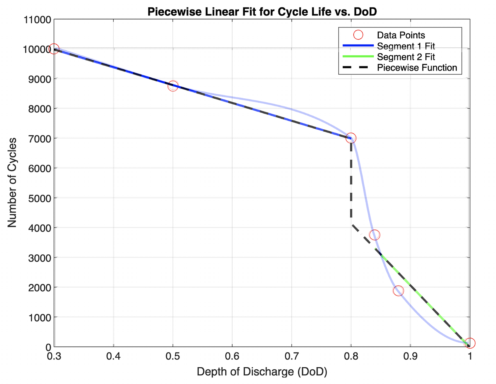
Figure 21: Interpolated Curve for Cycle Life vs. DoD

In this model, a DoD over 80% is avoided according to Ref. [16], therefore the model is reduced to:

$$N_{cycles}(\text{DoD})=a_{1}\cdot DoD+b_{1}$$ (118)

This is further adjusted by the following, assuming that the charge rates are linked to the cycles via a power ratio:

$$N_{\text{cycles}}=N_{\text{cycles}}(\text{DoD})\cdot\left(\frac{1}{\text{C-rate}_{\text{discharge}}^{c}}\right)\cdot\left(\frac{0.5}{\text{C-rate}_{\text{charge}}^{d}}\right)$$

Where:

• $a_{1},b_{1},a_{2},b_{2}$ are the fitted parameters for the piecewise linear segments.

• $c=1.1$ and $d=1.2$ are empirically estimated coefficients that account for the effects of discharging and charging rates, respectively.

• Fitted Parameters:

  $$\text{For DoD}\leq 0.8:a_{1}=-5986.8421,b_{1}=11776.3158$$

  $$\text{For DoD}>0.8:a_{2}=-20793.2692,b_{2}=20769.2307$$

This results in the follwing used equation:

$$N_{\text{cycles}}=(-5986.8421\cdot DoD+11776.3158)\cdot\left(\frac{1}{\text{C-rate}_{\text{discharge}}^{1.1}}\right)\cdot\left(\frac{0.5}{\text{C-rate}_{\text{charge}}^{1.2}}\right)$$ (119)

With:

• Discharge Rate: $C-{rate_{discharge}}=\frac{C_{\text{rate\_hover}}\cdot t_{\text{hover}}+C_{\text{rate\_climb}}\cdot t_{\text{cl}}+C_{\text{rate\_cruise}}\cdot t_{\text{cr}}}{t_{\text{tot}}}$: Average C-rate across the different phases of flight.

• $C_{\text{rate\_hover}}=\frac{\text{Power}_{\text{hover}}}{E_{\text{battery}}}$: C-rate during hover, defined as the ratio of hover power to total battery energy.

• $C_{\text{rate\_climb}}=\frac{\text{Power}_{\text{climb}}}{E_{\text{battery}}}$: C-rate during climb, defined as the ratio of climb power to total battery energy.

• $C_{\text{rate\_cruise}}=\frac{\text{Power}_{\text{cruise}}}{E_{\text{battery}}}$: C-rate during cruise, defined as the ratio of cruise power to total battery energy.

• $E_{\text{battery}}=\rho_{\text{bat}}\cdot m_{\text{bat}}$: Total energy capacity of the battery in Wh.

• Charge Rate: $C-rate_{charge}$ is assumed to be a design variable within the framework, so set fixed and changed as required.

• DoD: $DOD=\frac{E_{trip}}{E_{Battery}}$, ratio of energy used to total stored energy.

The resultant battery cycle-life envelope is illustrated in Fig. (22) for a constant $C-rate_{charge}$ of 2C. The empirical model developed provides a first estimation of battery cycle life across different DoD and C-rate conditions, based on battery data. The piecewise linear approach effectively captures the sharp decrease in cycle life observed at higher DoD levels.

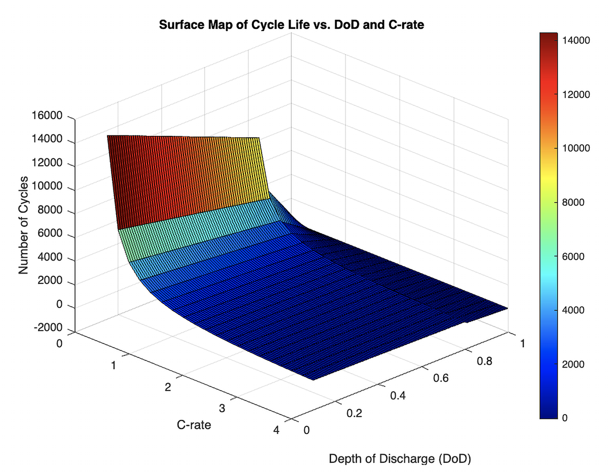
Figure 22: Piecewise Linear Fit for Cycle Life vs. DoD

B.5.2 Method 2

Assumptions and Limitations:

• This method delivers a simpler and static approach for battery cycle-life estimation, making the model less dynamic.

From Ref. [19] the average degradation of the battery per charging cycle is $Q_{cycle}=0.048\%$. Assuming an allowed degradation of $D=20\%$, the number of life cycles for the eVTOL is:

$$N_{cycles}=\frac{D}{Q}=\frac{20}{0.048}=416.67$$ (120)

B.6 Constraint Model

B.6.1 Wing-Rotor Geometry Constraint

The lifting rotor radius tends to reach the upper limit during optimization design because a lower disk loading reduces power consumption [8]. A geometry constraint is implemented to prevent interferences between the lifting rotors, their attachment to the wings and minimum distances between the lifting rotors and between the lifting rotors and the fuselage ($d$), where the fuselage width is $w$. $d$ is set fix to 0.0125m, as required by EASA, Ref. [47]. This condition applies to both the rotor radii $R_{prop_{hover}}$ and the span $b$. Eq. 121 and 122 are based on an lift plus cruise condition with 8 lifting rotors, as used in the demonstrated framework. Eq. 123 illustrates this approach for an undefined number of lifting rotors, but only considers $n_{lifter}\geq 4$ and $n_{lifter}\in 4\mathbb{Z}$ Fig. 23 illustrates this restriction.

$$\text{Wingspan Condition: }\frac{b}{2}\geq(3\cdot R_{prop_{hover}}+2\cdot d+\frac{w}{2})$$ (121)

resulting in minimum wing span $b_{min}$,

$$b_{min}=2\cdot(3\cdot R_{prop_{hover}}+2\cdot d+\frac{w}{2})$$ (122)

or for undefined number of rotors:

$$b_{min}=2\cdot\left(\left(\frac{1}{4}\cdot n_{lifter}\cdot 2\cdot R_{prop_{hover}}-R_{prop_{hover}}\right)+\frac{1}{4}\cdot n_{lifter}\cdot d+\frac{w}{2}\right)$$ (123)

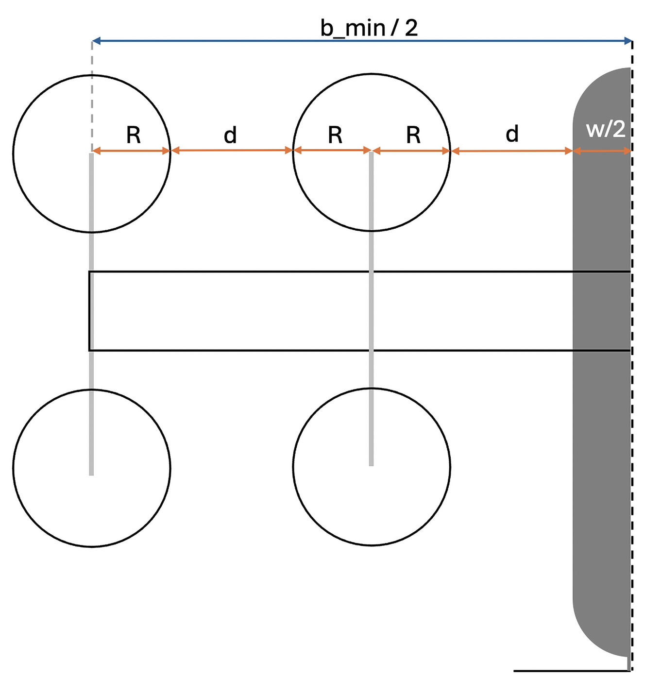
Figure 23: Geometry constraint on minimal wing span, lifting rotor and fuselage interference

B.6.2 Vertiport Constraint

Since the construction of new vertiports involves considerable financial investment and in many cases complex authorization procedures, a successful initial eVTOL operation can be planned on the basis of a design that meets the requirements of existing heliports. According an author-led expert interview with the helipad data provider "Helipaddy", the average $D$-value for existing helipads, potentially be used for UAM-operations, can be assumed for 15m. Therefore, this is assumed to be the maximum dimension of the EVTOL to maximize the likelihood of successful integration into existing air traffic infrastructure. This constraint is expressed in the following equations, where $R_{prop_{hover}}$ is the lifting rotor radius, $d$ is the distance between lifting rotors and fuselage, $w$ is the width of the fuselage, $b$ is the eVTOL wing span:

$$\text{Vertiport Constraint: }18\geq 2\cdot(2\cdot d+4\cdot R_{prop_{hover}}+\frac{w}{2})$$ (124)

$$\text{Vertiport Constraint: }15\geq b$$ (125)

Within the demonstrated framework it is assumed that $d=0.2m$ and $w=1.5m$. Fig. (24) illustrates the D-value, defined by EASA, Ref. [58], as the minimum space needed for an eVTOL to land, taxi, and park. If an eVTOL’s D-value exceeds the as average assumed 15m, it may not fit within existing heliports, necessitating larger or specially designed vertiports. This will impacts the design and adaptability of vertiport infrastructure.

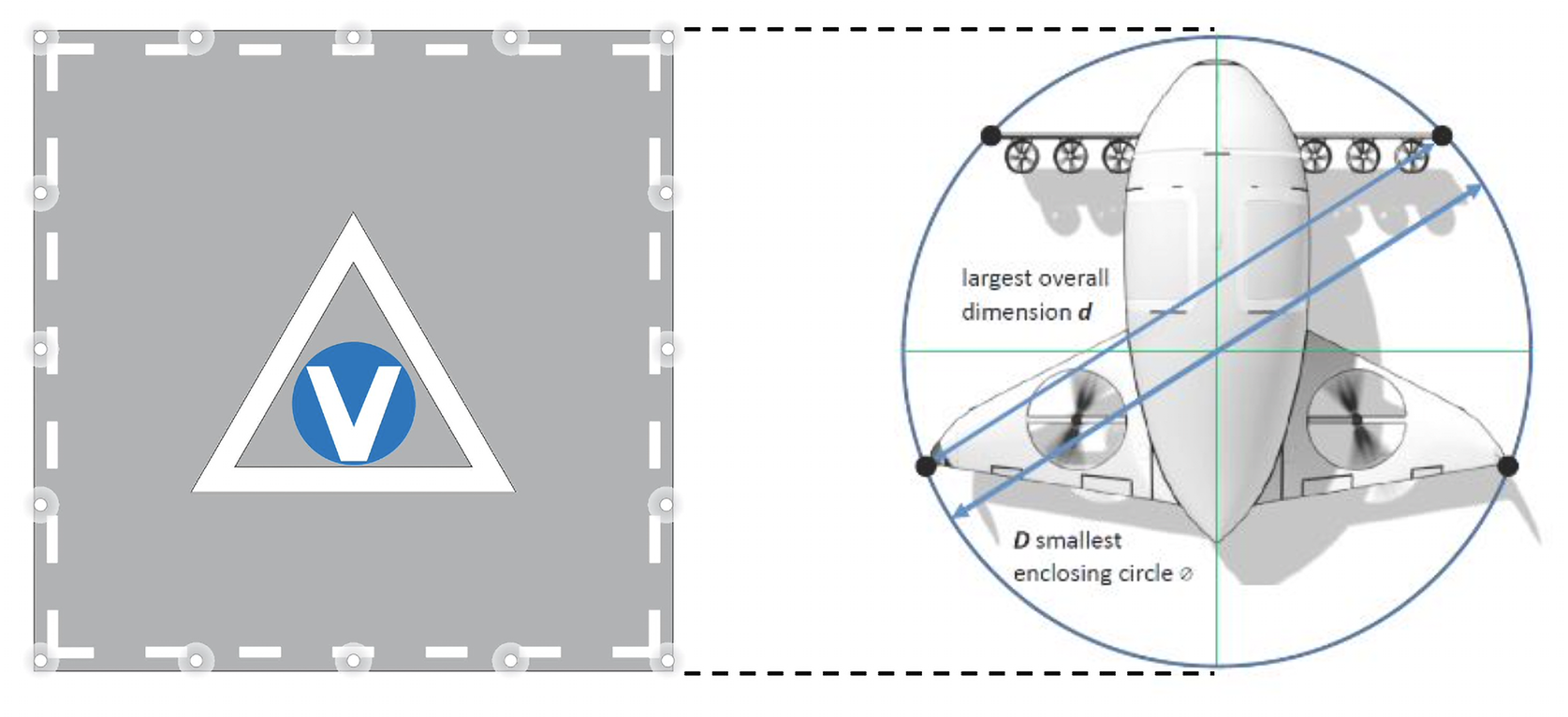
Figure 24: D-value for Vertiports, from Ref. [58].

References

- [1] Lukas Kiesewetter, Kazi Hassan Shakib, Paramvir Singh, Mizanur Rahman, Bhupendra Khandelwal, Sudarshan Kumar, and Krishna Shah. A holistic review of the current state of research on aircraft design concepts and consideration for advanced air mobility applications. Progress in Aerospace Sciences, 142:100949, 2023.
- [2] A. W. Schäfer, S. R. H. Barrett, K. Doyme, L. M. Dray, A. R. Gnadt, R. Self, et al. Technological, Economic and Environmental Prospects of All-electric Aircraft. Springer Science and Business Media LLC, 2018.
- [3] European Union Aviation Safety Agency (EASA). Study on the societal acceptance of urban air mobility in europe. Available online: https://www.easa.europa.eu/sites/default/files/dfu/uam-full-report.pdf, May 2021. This study has been carried out for EASA by McKinsey & Company.
- [4] NASA Aeronautics Research Mission Directorate. Urban Air Mobility Reference Material. Available online: https://sacd.larc.nasa.gov/uam-refs/, 2024. Accessed: 2024-06-01.
- [5] DFS Deutsche Flugsicherung GmbH and SkyVector. Aviation navigation resources: Dfs aip and skyvector. Available online: DFS AIP (https://aip.dfs.de/basicAIP/), SkyVector (https://skyvector.com), 2024. Accessed: 2024-12-20.
- [6] Shugo Kaneko and Joaquim R.R.A. Martins. Simultaneous optimization of design and takeoff trajectory for an evtol aircraft. Aerospace Science and Technology, 155:109617, 2024.
- [7] D. Sarojini, M. L. Ruh, A. J. Joshy, J. Yan, A. K. Ivanov, L. Scotzniovsky, et al. Large-Scale Multidisciplinary Design Optimization of an eVTOL Aircraft using Comprehensive Analysis. American Institute of Aeronautics and Astronautics, 2023.
- [8] Joaquim R. R. A. Martins and Andrew Ning. Engineering Design Optimization. Cambridge University Press, 2021.
- [9] M. L. Ruh, A. Fletcher, D. Sarojini, M. Sperry, J. Yan, L. Scotzniovsky, et al. Large-scale Multidisciplinary Design Optimization of a NASA Air Taxi Concept using a Comprehensive Physics-based System Model. American Institute of Aeronautics and Astronautics, 2024.
- [10] D. Keijzer, C. Simon Soria, J. Arends, B. Sarigol, F. Scarano, and S. G. Castro. Design of a Hydrogen-Powered Crashworthy eVTOL Using Multidisciplinary Analysis and Design Optimization. American Institute of Aeronautics and Astronautics, 2024.
- [11] T. H. Ha, K. Lee, and J. T. Hwang. Large-scale design-economics optimization of evtol concepts for urban air mobility, 2019. 10.2514/6.2019-1218.
- [12] P. K. Chinthoju, Y. H. Lee, G. K. Das, K. A. James, and J. T. Allison. Optimal Design of eVTOLs for Urban Mobility using Analytical Target Cascading (ATC). American Institute of Aeronautics and Astronautics, 2024.
- [13] A. Brown and W. L. Harris. A vehicle design and optimization model for on-demand aviation. AIAA/ASCE/AHS/ASC Structures, Structural Dynamics, and Materials Conference, 2018.
- [14] Michael D. Patterson, Kevin R. Antcliff, and Lee W. Kohlman. A proposed approach to studying urban air mobility missions including an initial exploration of mission requirements. Available online: https://ntrs.nasa.gov/api/citations/20190000991/downloads/20190000991.pdf, 2018.
- [15] Carlos Silva, Wayne Johnson, Ken Antcliff, and Michael D. Patterson. Vtol urban air mobility concept vehicles for technology development, 2018.
- [16] Chi Yang, Yuchen Gao, Weigang Wei, Chang Liu, Kai Wang, Yue Zhang, Haiping Liu, Xiaoqing Lu, Fei Ren, Yuyi Yang, Kejie Li, and Xinfeng Zhao. Challenges and key requirements of batteries for electric vertical takeoff and landing aircraft. Joule, 5(8):1884–1900, 2021. Accessed: 2024-06-12.
- [17] Aishwarya Kasliwal, Nicholas J. Furbush, John H. Gawron, James R. McBride, Timothy J. Wallington, Robert D. De Kleine, et al. Role of Flying Cars in Sustainable Mobility. Springer Science and Business Media LLC, 2019.
- [18] N. André and M. Hajek. Robust Environmental Life Cycle Assessment of Electric VTOL Concepts for Urban Air Mobility. American Institute of Aeronautics and Astronautics, 2019.
- [19] Y. Mihara, P. Pawnlada, A. Nakamoto, T. Nakamura, M. Nakano, and P. Pawnlanda. Cost analysis of evtol configuration design for an air ambulance system in japan. Journal of Advanced Transportation, 2021:Article ID 8821234, 2021. Available online.
- [20] Y. Liu and C. Gao. Assessing Electric Vertical Take-Off and Landing for Urban Air Taxi Services: Key Parameters and Future Transportation Impact. MDPI AG, 2024.
- [21] F. Arshad, J. Lin, N. Manurkar, E. Fan, A. Ahmad, M. Tariq, et al. Life cycle assessment of lithium-ion batteries: A critical review. Resources, Conservation and Recycling, 180, 2022.
- [22] H. B. Faulkner. The ata-67 formula for direct operating cost. Available online: https://ntrs.nasa.gov/api/citations/19730024119/downloads/19730024119.pdf, May 1973.
- [23] Jeff Holden and Nikhil Goel. Fast-forwarding to a future of on-demand urban air transportation. Available online: https://evtol.news/__media/PDFs/UberElevateWhitePaperOct2016.pdf, 2016.
- [24] A. B. Lambe and J. R. R. A. Martins. Extensions to the design structure matrix for the description of multidisciplinary design, analysis, and optimization processes. Structural and Multidisciplinary Optimization, 46(2):273–284, 2012.
- [25] Tecnam. P2006t aircraft manual. https://tecnam.com/wp-content/uploads/2015/05/P2006T-14-w.pdf, 2014. Accessed: 2024-08-29.
- [26] European Union Aviation Safety Agency (EASA). Special condition for small-category vtol-capable aircraft, issue 2. Available online: https://www.easa.europa.eu/sites/default/files/dfu/sc-vtol-issue-2.pdf, June 2024. Accessed: 2024-06-10.
- [27] Fuelbirds. Helicopter pads and helipads: How to select the right one for your needs. Available online: https://www.fuelbirds.com/helicopter-pads-and-helipads-how-to-select-the-right-one-for-your-needs/, 2023. Accessed: 2024-07-17.
- [28] European Union Aviation Safety Agency (EASA). SERA.5005 Visual Flight Rules. Available online: https://eur-lex.europa.eu/legal-content/EN/TXT/?uri=CELEX%3A32016R1185, 2016. Regulation (EU) 2016/1185, Accessed: 2024-06-23.
- [29] European Union Aviation Safety Agency. Special condition vtol. Available online: https://www.easa.europa.eu/en/document-library/product-certification-consultations/special-condition-vtol, 2024. Accessed: 2024-06-12.
- [30] Daniel P. Raymer. Aircraft Design: A Conceptual Approach. AIAA Education Series. American Institute of Aeronautics and Astronautics, 2nd edition, 1992.
- [31] Snorri Gudmundsson. General Aviation Aircraft Design: Applied Methods and Procedures. Butterworth-Heinemann, 2013. Accessed: 2024-08-08.
- [32] European Union Aviation Safety Agency. EASA review of standard passenger weights 2022 shows no significant change. Available online: https://www.easa.europa.eu/en/newsroom-and-events/news/easa-review-standard-passenger-weights-2022-shows-no-significant-change, 2022. Accessed: 2024-06-12.
- [33] B. Govindarajan and A. Sridharan. Conceptual sizing of vertical lift package delivery platforms. Journal of Aircraft, 57(6):1170, 2020.
- [34] S. S. Chauhan and J. R. R. A. Martins. Tilt-wing evtol takeoff trajectory optimization. Journal of Aircraft, 57(1):93, 2019.
- [35] Airfoil Tools. Naca airfoil polars (naca 0012, naca 2412). Available online: NACA 0012 (http://airfoiltools.com/polar/details?polar=xf-n0012-il-200000), NACA 2412 (http://airfoiltools.com/polar/details?polar=xf-naca2412-il-200000), 2024. Accessed: 2024-07-16.
- [36] Uber Elevate. Summary of mission and requirements for uberair vehicles. Available online: https://s3.amazonaws.com/uber-static/elevate/Summary+Mission+and+Requirements.pdf, December 2023. Accessed: 2024-06-23.
- [37] International Civil Aviation Organization (ICAO). Airlines operating costs and productivity. Available online: https://www.icao.int/mid/documents/2017/aviation%20data%20and%20analysis%20seminar/ppt3%20-%20airlines%20operating%20costs%20and%20productivity.pdf, 2017. Accessed: 2024-06-16.
- [38] Investopedia. Annuity method of depreciation. https://www.investopedia.com/terms/a/annuity-method-of-depreciation.asp#:~:text=The%20annuity%20method%20of%20depreciation%20is%20a%20process%20used%20to,least%20constant)%20rate%20of%20return., 2023. Accessed: 2024-06-15.
- [39] Taxi fare calculator london. https://www.bettertaxi.com/taxi-fare-calculator/london/. Accessed: 2024-08-19.
- [40] International Energy Agency (IEA). Germany - countries & regions. https://www.iea.org/countries/germany, 2024. Accessed: 2024-08-29.
- [41] IPCC. Annex iii: Technology-specific cost and performance parameters. https://www.ipcc.ch/site/assets/uploads/2018/02/ipcc_wg3_ar5_annex-iii.pdf, 2014. Accessed: 2024-08-29.
- [42] World Nuclear Association. Carbon dioxide emissions from electricity, 2024. Accessed: 2024-08-29.
- [43] Bjorn Fehrm. Bjorn corner: Sustainable air transport. part 43. evtol ifr range. Available online: https://leehamnews.com/2022/10/28/bjorns-corner-sustainable-air-transport-part-43-evtol-ifr-range/, 2022. Accessed: 2024-08-29.
- [44] Patrick Wills. Expert interview/correspondence with helipaddy limited founder. Email, 2024. Average existing helipad dimension for UAM can be assumed to be 15m.
- [45] Airbus. Extra performance wing demonstrator takes off. Available online: https://www.airbus.com/en/newsroom/stories/2023-11-extra-performance-wing-demonstrator-takes-off, 2023. Accessed: 2023-11-12.
-
[46]
MT-Propeller.
Technical Data Sheets for MTV Series Propellers.
- •
- •
- •
- •
- •
- [47] European Union Aviation Safety Agency (EASA). Easy Access Rules for Large Aeroplanes (CS-25)-CS 25.925. Available online: https://www.easa.europa.eu/en/document-library/easy-access-rules/online-publications/easy-access-rules-large-aeroplanes-cs-25?kw=propeller%20clearance, note = Accessed: August 10, 2024, 2024. Accessed: August 10, 2024.
- [48] Federal Aviation Administration. 14 cfr § 25.925 - propeller clearance. Available online: https://www.ecfr.gov/current/title-14/chapter-I/subchapter-C/part-25/subpart-E/subject-group-ECFR3db216ad9d52259/section-25.925, 2024. Accessed: August 10, 2024.
- [49] Alessandro Bacchini, Enrico Cestino, Benjamin Van Magill, and Dries Verstraete. Impact of lift propeller drag on the performance of evtol lift+cruise aircraft. Aerospace Science and Technology, 109:106429, 2021.
- [50] Constantin Rotaru and Michael Todorov. Helicopter Flight Physics. IntechOpen, February 2018. Licensed under CC BY 4.0.
- [51] James F. Marchman III. Altitude Change: Climb and Glide, chapter 5. James F. Marchman III in association with the University Libraries at Virginia Tech, 2021.
- [52] H. B. Faulkner. The ata-67 formula for direct operating cost. Available online: https://ntrs.nasa.gov/api/citations/19730024119/downloads/19730024119.pdf, May 1973. NASA Technical Memorandum.
- [53] DFS Deutsche Flugsicherung. Charges - legal framework. Available online: https://www.dfs.de/homepage/en/air-traffic-control/legal-framework/charges/, 2024. Accessed: 2024-06-15.
- [54] Economic Research Institute (ERI). Helicopter pilot salary in germany. Available online: https://www.erieri.com/salary/job/helicopter-pilot/germany#:~:text=The%20average%20salary%20range%20for,conducted%20and%20researched%20by%20ERI., 2024. Accessed: 2024-06-15.
- [55] Valor International. Orders for eve’s flying car total $8.3bn. Available online: https://valorinternational.globo.com/business/news/2023/05/02/orders-for-eves-flying-car-total-83bn.ghtml, 2023. Accessed: 2024-06-15.
- [56] Michael J. Duffy, Sean Wakayama, Ryan Hupp, Roger Lacy, and Matt Stauffer. A study in reducing the cost of vertical flight with electric propulsion. In American Institute of Aeronautics and Astronautics Conference. The Boeing Company, 2017. Accessed: 2024-08-13.
- [57] Chris Wetherell. Let’s talk about the panasonic ncr18650b. Available online: https://turtleherding.com/wp-content/uploads/2018/06/Lets-talk-about-the-Panasonic-NCR18650B.pdf, 2018. Accessed: 2024-08-13.
- [58] European Union Aviation Safety Agency (EASA). Prototype Technical Specifications for the Design of VFR Vertiports for Operation with Manned VTOL-Capable Aircraft Certified in the Enhanced Category (PTS-VPT-DSN). Available online: https://www.easa.europa.eu/en/document-library/general-publications/prototype-technical-design-specifications-vertiports, March 2022. Non-binding guidance material for vertiport design and operation.