Maximal number of mixed Nash equilibria in generic games where each player has two pure strategies

Abstract.

The number of Nash equilibria of the mixed extension of a generic finite game in normal form is finite and odd. This raises the question how large the number can be, depending on the number of players and the numbers of their pure strategies. Here we present a lower bound for the maximal possible number in the case of $m$-player games where each player has two pure strategies. It is surprisingly close to a known upper bound.

1. Main result and its context

The set ${\mathcal{N}}$ of Nash equilibria of the mixed extension of a finite game in normal form is non-empty. This was proved by Nash [Na51], and it was one early instance of the relevance of the notion of Nash equilibria. A natural question is how the set ${\mathcal{N}}$ might look like. For generic games, it was shown by Wilson [Wi71], Rosenmüller [Ro71] and Harsanyi [Ha73] that ${\mathcal{N}}$ is finite and odd. For arbitrary games, ${\mathcal{N}}$ is a real semialgebraic set and can look arbitrarily complicated [Da03].

Here we focus on the case of generic games and ask about the maximum of the numbers $|{\mathcal{N}}|$ for generic games with fixed numbers of players and of pure strategies. This is not of immediate use in applications in economics, but it is useful in order to estimate the complexity of the problem of controlling ${\mathcal{N}}$.

We consider finite games with a fixed number $m$ of players $i\in{\mathcal{A}}=\{1,...,m\}$ where each player has a fixed set $S^{i}=\{s^{i}_{0},s^{i}_{1},...,s^{i}_{n_{i}}\}$ of pure strategies. The set $S=S^{1}\times...\times S^{m}$ is the set of all pure strategy combinations. Each player has a utility function $U^{i}:S\to{\mathbb{R}}$. These combine to a utility map $U=(U^{1},...,U^{m}):S\to{\mathbb{R}}^{m}$. A game is generic if $U$ is generic. In the mixed extension $({\mathcal{A}},G,V)$, the set $G^{i}$ of mixed strategies of player $i$ is the simplex of probability distributions over $S^{i}$, and $V:G\to{\mathbb{R}}^{m}$ is the multilinear extension of $U$ to $G=G^{1}\times...\times G^{m}$ (see the formula (2.1)). We denote by $\mu(m;n_{1}+1,...,n_{m}+1)\in{\mathbb{N}}$ the maximal number of mixed Nash equilibria within all games $({\mathcal{A}},S,U)$ with fixed sets ${\mathcal{A}}$ and $S$ and generic $U$.

In most cases this number is unknown. In the case of two players an upper bound was given by Keiding [Ke97], and in the case of two players and $n_{1}=n_{2}$ a lower bound was given by von Stengel [St97][St99]. Their asymptotics for large $n_{1}+1=n_{2}+1=n$ are roughly as follows,

$$0.95\frac{2.4^{n}}{\sqrt{n}}\leq\mu(2;n,n)\leq 0.92\frac{2.6^{n}}{\sqrt{n}} \textup{if }n\textup{ is even,}$$

$$0.67\frac{2.4^{n}}{\sqrt{n}}\leq\mu(2;n,n)\leq 0.8\frac{2.6^{n}}{\sqrt{n}} \textup{if }n\textup{ is odd.}$$

The only known numbers $\mu(2;n,n)$ are [Ke97][MP99]

$$(\mu(2;n,n)\,|\,n\in\{1,2,3,4\})=(1,3,7,15).$$

Though $\mu(2;6,6)\geq 75>63$ [St97][St99]. This refuted the conjecture $\mu(2;n,n)\stackrel{{\scriptstyle?}}{{=}}2^{n}-1$ of Quint and Shubik [QS97].

For more than two players, little is known. The best result is due to McKelvey and McLennan [MM97]. They considered totally mixed Nash equilibria (TMNE), which are Nash equilibria in the interior of $G$, so that any pure strategy has positive probability. They found that the maximal number of TMNE for generic games $({\mathcal{A}},S,U)$ as above is the number $E(m;n_{1},...,n_{m})$ of block derangements: It is the number of partitions of the set $\bigcup_{i\in{\mathcal{A}}}(S^{i}-\{s^{i}_{0}\})$ into new sets $B^{1},...,B^{m}$ with $|B^{i}|=n_{i}$ and $B^{i}\cap(S^{i}-\{s^{i}_{0}\})=\emptyset$. They and Vidunas [Vi17] studied these numbers. Vidunas derived from this a rough upper bound for $\mu(m;n_{1}+1,...,n_{m}+1)$ in the general case: As each Nash equilibrium is a TMNE of the restricted game where only those pure strategies are considered which have positive probability in the given Nash equilibrium, one finds

$$\mu(m;n_{1}+1,...,n_{m}+1)$$

$$\leq\sum_{(k_{1},...,k_{m})\in\prod_{i\in{\mathcal{A}}}\{0,1,...,n_{i}\}}\begin{pmatrix}n_{1}+1\\ k_{1}+1\end{pmatrix}...\begin{pmatrix}n_{m}+1\\ k_{m}+1\end{pmatrix}E(m;k_{1},...,k_{m}).\hskip 28.45274pt$$ (1.1)

Vidunas [Vi17] proved that the right hand side is equal to the number

$$\sum_{(k_{1},...,k_{m})\in\prod_{i\in{\mathcal{A}}}\{0,1,...,n_{i}\}}\frac{(k_{1}+...+k_{m})!}{k_{1}!\cdot...\cdot k_{m}!}.\hskip 28.45274pt$$ (1.2)

In general, this upper bound is coarse. For example, for $\mu(2;n,n)$ it gives an upper bound with the asymptotics $4^{n}/\sqrt{\pi n}$, which is much coarser than Keiding’s upper bound.

In this paper we focus on the number $\mu(m;2,...,2)$, so many players with two strategies each, which is quite opposite to the case of two players with many strategies each. There the number of block derangements specializes to the number

$$!m:=E(m;1,...,1)=|\{\sigma\in S_{m}\,|\,\textup{Fix}(\sigma)=\emptyset\}|$$ (1.3)

of derangements (permutations without fixed points). Vidunas’ upper bound specializes to

$$\mu(m;2,...,2)\leq V(m):=\sum_{l=0}^{m}\begin{pmatrix}m\\ l\end{pmatrix}\cdot 2^{l}\cdot!(m-l)\stackrel{{\scriptstyle\eqref{1.1}=\eqref{1.2}}}{{=}}\sum_{l=0}^{m}\frac{m!}{l!}.$$ (1.4)

Our main result is the lower bound

$$\frac{1}{2}(V(m)+!m)\leq\mu(m;2,...,2).$$ (1.5)

This is more than half of the upper bound $V(m)$, so it is remarkably close to the upper bound. For example

$$\begin{array}[]{c|c|c|c|c|c}m&2&3&4&5\\ \hline\cr V(m)&5&16&65&326\\ \hline\cr\frac{1}{2}(V(m)+!m)&3&9&37&187\end{array}$$

We even conjecture equality in (1.5) (see section 5).

Section 2 sets the notations for arbitrary finite games and their mixed extensions. Section 3 studies games with $n_{1}=...=n_{m}=2$, it introduces a special subfamily of non-generic games, and it gives general results on their Nash equilibria and equilibrium candidates. It sets the stage for Section 4. Section 4 proves that this subfamily contains games with $\frac{1}{2}(V(m)+!m)$ Nash equilibria. The art is to control simultaneously Nash equilibria with all different possible supports. This leads to interesting combinatorics. Section 5 formulates a conjecture which refines the conjecture that equality holds in (1.5).

2. The mixed extension of a finite game

In this section, a finite game in normal form, its mixed extension, best reply maps, Nash equilibria and equilibrium candidates are introduced formally.

Definition 2.1.

(a) $({\mathcal{A}},S,U)$ denotes a finite game as in the Introduction. So here $m\in{\mathbb{N}}=\{1,2,3,...\}$, ${\mathcal{A}}:=\{1,...,m\}$ is the set of players, $S^{i}=\{s^{i}_{0},...,s^{i}_{n_{i}}\}$ is the set of pure strategies of player $i\in{\mathcal{A}}$, $S=S^{1}\times...\times S^{m}$ is the set of pure strategy combinations, $U^{i}:S\to{\mathbb{R}}$ is the utility function of player $i$, and $U=U^{1}\times...\times U^{m}:S\to{\mathbb{R}}^{m}$. The pure strategy combinations are given as tuples $(s^{1}_{j_{1}},...,s^{m}_{j_{m}})\in S$ with $(j_{1},...,j_{m})\in J:=\prod_{i\in{\mathcal{A}}}\{0,1,...,n_{i}\}$.

(b) $({\mathcal{A}},G,V)$ denotes the mixed extension of the finite game in (a). Here

$$W^{i}:=\bigoplus_{j=0}^{n_{i}}{\mathbb{R}}\cdot s^{i}_{j}, W:=W^{1}\times...\times W^{m},$$

$$A^{i}:=\{\sum_{j=0}^{n_{i}}\gamma^{i}_{j}s^{i}_{j}\in W^{i}\,|\,\sum_{j=0}^{n_{i}}\gamma^{i}_{j}=1,\}, A:=A^{1}\times...\times A^{m}\subset W,$$

$$G^{i}:=\{\sum_{j=0}^{n_{i}}\gamma^{i}_{j}s^{i}_{j}\in A^{i}\,|\,\gamma^{i}_{j}\in[0,1],\}, G:=G^{1}\times...\times G^{m}\subset A.$$

So, $W^{i}$ and $W$ are real vector spaces, $A^{i}\subset W^{i}$ and $A\subset W$ are affine linear subspaces of codimension $1$ respectively $m$, $G^{i}\subset A^{i}$ is a simplex in $A^{i}$ of the same dimension $n_{i}$ as $A^{i}$, and $G\subset A$ is a product of simplices, so especially a convex polytope, and it has the same dimension $\sum_{i=1}^{m}n_{i}$ as $A$. The map $V^{i}_{W}:W\to{\mathbb{R}}^{m}$ is the multilinear extension of $U^{i}$,

$$V^{i}_{W}(g) := \sum_{(j_{1},...,j_{m})\in J}\Bigl{(}\prod_{k=1}^{m}\gamma^{k}_{j_{k}}\Bigr{)}\cdot U^{i}(s^{1}_{j_{1}},...,s^{m}_{j_{m}}),$$ (2.1)

$$\textup{where}\quad g = (g^{1},...,g^{m})\in W\textup{ with }g^{k}=\sum_{j=0}^{n_{k}}\gamma^{k}_{j}s^{k}_{j}.$$

$V^{i}_{A}:A\to{\mathbb{R}}$ is the restriction of $V^{i}_{W}$ to $A$, and $V^{i}:G\to{\mathbb{R}}$ is the restriction of $V^{i}_{W}$ to $G$. Then $V=(V^{1},...,V^{m}):G\to{\mathbb{R}}^{m}$. An element $g\in G$ is called a mixed strategy combination. The support of an element

$$g^{i}=\sum_{j=0}^{n_{i}}\gamma^{i}_{j}s^{i}_{j}\in W^{i}\quad\textup{is the set}\quad{\rm supp}(g^{i}):=\{j\in\{0,1,...,n_{i}\}\,|\,\gamma^{i}_{j}\neq 0\}.$$

The support of $g\in W$ is ${\rm supp}(g)=\prod_{i\in{\mathcal{A}}}{\rm supp}(g^{i})\subset J$. We also denote $W^{-i}:=W^{1}\times...\times W^{i-1}\times W^{i+1}\times...\times W^{m}$, its elements $g^{-i}:=(g^{1},...,g^{i-1},g^{i+1},...,g^{m})\in W^{-i}$, and analogously $A^{-i}$ and $G^{-i}$. We follow the standard (slightly incorrect) convention and identify $W^{i}\times W^{-i}$ with $W$, $A^{i}\times A^{-i}$ with $A$, $G^{i}\times G^{-i}$ with $G$ and $(g^{i},g^{-i})$ with $g$.

(c) Fix $i\in{\mathcal{A}}$. The best reply map $r^{i}:G^{-i}\to{\mathcal{P}}(G^{i})$ associates to each element $g^{-i}\in G^{-i}$ the set of its best replies in $G^{i}$,

$$r^{i}(g^{-i}):=\{g^{i}\in G^{i}\,|\,V^{i}(\widetilde{g}^{i},g^{-i})\leq V^{i}(g^{i},g^{-i})\textup{ for any }\widetilde{g}^{i}\in G^{i}\}.$$

Its graph is the set

$$\operatorname{Gr}(r^{i}):=\bigcup_{g^{-i}\in G^{-i}}r^{i}(g^{-i})\times\{g^{-i}\}\subset G^{i}\times G^{-i}=G.$$

A Nash equilibrium is an element of the set ${\mathcal{N}}:=\bigcap_{i\in{\mathcal{A}}}\operatorname{Gr}(r^{i})$. The set ${\mathcal{N}}$ is the set of all Nash equilibria. A TMNE (totally mixed Nash equilibrium) is a Nash equilibrium $g$ with ${\rm supp}(g)=J$.

Remark 2.2.

For $({\mathcal{A}},G,V)$ as above, define a function $\lambda^{i}_{j}:A^{-i}\to{\mathbb{R}}$ for $i\in{\mathcal{A}}$ and $j\in\{0,1,...,n_{i}\}$ by

$$\lambda^{i}_{j}(g^{-i}):=V^{i}_{A}(s^{i}_{j},g^{-i})-V^{i}_{A}(s^{i}_{0},g^{-i})\quad\textup{for }g^{-i}\in A^{-i},$$ (2.2)

so $\lambda^{i}_{0}=0$. Then $g$ is a Nash equilibrium if and only if $g\in G$ and for any $i\in{\mathcal{A}}$

$$\lambda^{i}_{j}(g^{-i})=\lambda^{i}_{k}(g^{-i}) \textup{for any }j,k\in{\rm supp}(g^{i}),$$ (2.3)

$$\textup{and }\lambda^{i}_{j}(g^{-i})\leq\lambda^{i}_{k}(g^{-i}) \textup{for any }j\notin{\rm supp}(g^{i}),\ k\in{\rm supp}(g^{i}).$$ (2.4)

This expresses the well known fact that for $g^{-i}\in G^{-i}$ the set $r^{i}(g^{-i})$ of best replies is the convex hull of the set $r^{i}(g^{-i})\cap S^{i}$ of pure best replies.

It motivates the definition of an equilibrium candidate.

Definition 2.3.

For $({\mathcal{A}},G,V)$ as above, a mixed strategy combination $g\in G$ is an equilibrium candidate if it satisfies (2.3) (but not necessarily (2.4)).

3. Product two-action games

From now on, we focus on finite games (and their mixed extensions) where each player has two pure strategies. First we give a name to such games (two-action games) and talk about coordinates on the affine space $A$ (see Definition 2.1 (b)). Then we recall the notion of derangements, which will be useful later. The main point in this section is the study of a special class of games (which we call product two-action games) where we have the maximal number of equilibrium candidates and can understand well which of them are Nash equilibria. Theorem 3.7 will formulate this precisely.

Definition 3.1.

(a) A two-action game is a mixed extension $({\mathcal{A}},G,V)$ of a finite game with $n_{1}=...=n_{m}=1$. Then we write $\gamma^{i}$ instead of $\gamma^{i}_{1}$ and $\lambda^{i}$ instead of $\lambda^{i}_{1}$. Recall $\lambda^{i}_{0}=0$. Here $\gamma^{i}$ is a coordinate on the 1-dimensional affine space $A^{i}\cong{\mathbb{R}}$. It identifies the subset $G^{i}$ with the interval with end points $0\sim s^{i}_{0}$ and $1\sim s^{i}_{1}$. The affine spaces $A$ and $A^{-i}$ come equipped with the coordinates $\underline{\gamma}=(\gamma^{1},...,\gamma^{m})$ and $\underline{\gamma}^{-i}=(\gamma^{1},...,\gamma^{i-1},\gamma^{i+1},...,\gamma^{m})$. With respect to these coordinates $G^{i}$, $G$ and $G^{-i}$ are identified with $[0;1]$, $[0;1]^{m}$ and $[0;1]^{m-1}$. The function $\lambda^{i}:A^{-i}\to{\mathbb{R}}$ is a polynomial in $\underline{\gamma}^{-i}$ such that each monomial in it has in each variable degree 0 or 1.

(b) For a two-action game and an element $g\in A$ write $L_{0}(g):=\{i\in{\mathcal{A}}\,|\,\gamma^{i}=0\}$, $L_{1}(g):=\{i\in{\mathcal{A}}\,|\,\gamma^{i}=1\}$, $L(g):=L_{0}(g)\cup L_{1}(g)$.

(c) For $L\subset{\mathcal{A}}$, the complementary set is $L^{\complement}:={\mathcal{A}}-L$. Let $|L|\in\{0,1,...,m\}$ be the number of elements of $L$.

In the study below of product two-action games, permutations without fixed points will be important.

Definition 3.2.

(a) A permutation $\pi\in S_{n}$ (for some $n\in{\mathbb{N}}$) is a derangement if $\pi(i)\neq i$ for any $i\in\{1,..,n\}$. The set of derangements in $S_{n}$ is called $\textup{Der}_{n}$. The subfactorial $!n$ is the number $|\textup{Der}_{n}|$ of derangements in $S_{n}$.

(b) For $\pi\in S_{n}$, denote by $F(\pi):=\{i\in{\mathcal{A}}\,|\,\pi(i)=i\}\subset{\mathcal{A}}$ the set of fixed points of $\pi$. Then $\pi$ restricted to $F(\pi)^{\complement}$ is a derangement on the set $F(\pi)^{\complement}$.

The subfactorial $!n$ can be determined in different ways. The following lemma collects three ways. It is completely elementary and well known, see e.g. [MM97, Proposition 5.4].

Lemma 3.3.

The subfactorials are determined by each of the recursions (3.1) and (3.2) and by the closed formula (3.3). The table (3.7) gives the first subfactorials and (for comparison) the first factorials.

$$!0=1,\ !n = n\cdot!(n-1)+(-1)^{n}\quad\textup{for }n\geq 1,$$ (3.1)

$$!0=1,\ !1=0,\ !n = (n-1)(!(n-1)+!(n-2))\quad\textup{for }n\geq 2,\hskip 28.45274pt$$ (3.2)

$$!n = n!\cdot\sum_{j=0}^{n}\frac{(-1)^{j}}{j!}\Bigl{(}=n!\cdot\sum_{j=2}^{n}\frac{(-1)^{j}}{j!}\Bigr{)}.$$ (3.3)

$$\begin{array}[]{r|r|r|r|r|r|r|r}n&0&1&2&3&4&5&6\\ \hline\cr!n&1&0&1&2&9&44&265\\ \hline\cr n!&1&1&2&6&24&120&720\end{array}$$ (3.7)

The closed formula (3.3) shows $\lim_{n\to\infty}\frac{!n}{n!}=e^{-1}$.

Definition 3.4.

(a) A two-action game $({\mathcal{A}},G,V)$ is product two-action, if each function $\lambda^{i}:A^{-i}\to{\mathbb{R}}$ has as a polynomial in $\underline{\gamma}^{-i}$ the shape

$$\lambda^{i}(\underline{\gamma}^{-i}) = (-1)^{v_{i}}\cdot\prod_{j\in{\mathcal{A}}-\{i\}}(\gamma^{j}-a^{i}_{j})$$ (3.8)

with suitable $a^{i}_{j}\in(0,1)$ and a suitable vector $\underline{v}=(v_{1},...,v_{m})\in\{0;1\}^{m}$, where $a^{i_{1}}_{j}\neq a^{i_{2}}_{j}$ for $j\in{\mathcal{A}}$ and $i_{1},i_{2}\in{\mathcal{A}}-\{j\}$ with $i_{1}\neq i_{2}$ is demanded.

(b) Let $({\mathcal{A}},G,V)$ be a product two-action game. For $j\in{\mathcal{A}}$, the unique permutation $\sigma^{j}\in S_{m}$ with

$$\sigma^{j}(j)=j,$$ (3.9)

$$1>a^{(\sigma^{j})^{-1}(1)}_{j}>...>a^{(\sigma^{j})^{-1}(j-1)}_{j}>a^{(\sigma^{j})^{-1}(j+1)}_{j}>...>a^{(\sigma^{j})^{-1}(m)}_{j}>0,$$

is called $j$-th associated permutation (to the product two-action game). The tuple $(\underline{v},\underline{\sigma})=(v_{1},...,v_{m},\sigma^{1},...,\sigma^{m})\in\{\pm 1\}^{m}\times(S_{m})^{m}$ is called characteristic tuple of the product two-action game.

Examples 3.5.

(i) Consider a two-action game with $m=3$ where $\lambda^{3}(g^{-3})=(\gamma^{1}-\frac{1}{2})(\gamma^{2}-\frac{1}{2})-\frac{1}{12}$. The zero set of $\lambda^{3}$ in $A^{1}\times A^{2}\cong{\mathbb{R}}^{2}$ is a hyperbola with asymptotics $\{\frac{1}{2}\}\times{\mathbb{R}}$ and ${\mathbb{R}}\times\{\frac{1}{2}\}$. The intersection $(\lambda^{3})^{-1}(0)|_{G^{1}\times G^{2}}$ of the two components with $G^{1}\times G^{2}\cong[0;1]^{2}$ splits the complement in $G^{1}\times G^{2}$ into two small regions near $(0,0)$ and $(1,1)$ and a large region in between. The graph $\operatorname{Gr}(r^{3})\subset G\cong[0;1]^{3}$ of the best reply map $r^{3}$ of player $3$ is the union of two top faces which are $(\textup{the two small regions})\times\{1\}$, a bottom face which is $(\textup{the large region})\times\{0\}$ and two vertical walls $(\lambda^{3})^{-1}(0)|_{G^{1}\times G^{2}}\times[0;1]$. See the left picture in Figure 1. The top and bottom faces are shaded darker, the walls are shaded brighter. Many more such pictures can be found in [JS22].

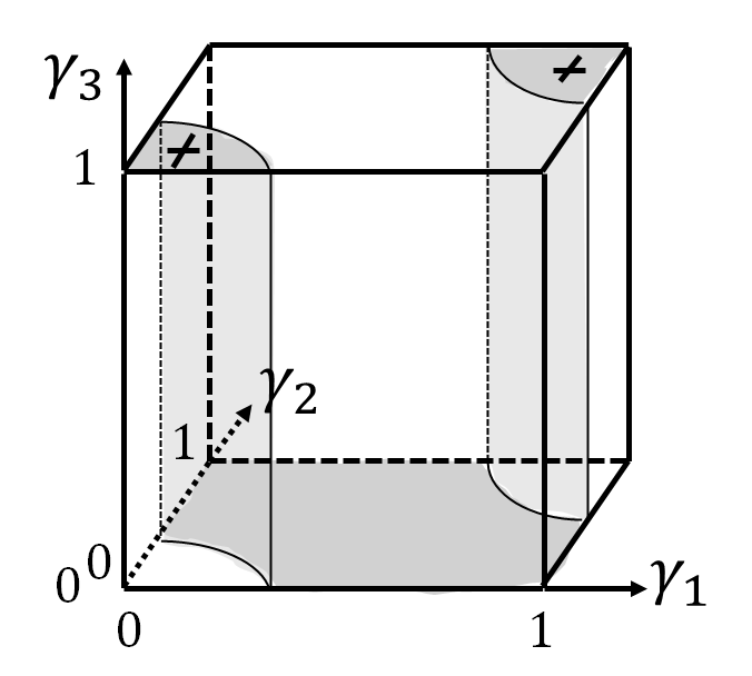
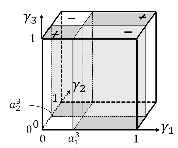
Figure 1. Left: $\operatorname{Gr}(r^{3})$ in (i). Right: $\operatorname{Gr}(r^{3})$ in (ii).

(ii) The best reply graph $\operatorname{Gr}(r^{3})$ in part (i) has a generic shape. In a product two-action game with $m=3$ andd $v_{3}=1$, $\lambda^{3}$ has the shape $\lambda^{3}(g^{-3})=(\gamma^{1}-a^{3}_{1})(\gamma^{2}-a^{3}_{2})$ with $a^{3}_{1},a^{3}_{2}\in(0;1)$. The zero set $(\lambda^{3})^{-1}(0)|_{G^{1}\times G^{2}}$ consists of the two lines $\{a^{3}_{1}\}\times[0;1]$ and $[0;1]\times\{a^{3}_{2}\}$. It splits the complement in $G^{1}\times G^{2}$ into four components, which are rectangles. The best reply graph $\operatorname{Gr}(r^{3})\subset G\cong[0;1]^{3}$ is the union of two top faces which are the two rectangles near $(0,0)$ and $(1,1)$ times $\{1\}$, two bottom faces which are the other two rectangles times $\{0\}$ and two vertical walls $\{a^{3}_{1}\}\times[0;1]^{2}$ and $[0;1]\times\{a^{3}_{2}\}\times[0;1]$. See the middle picture in Figure 1. The top and bottom faces are shaded darker, the walls are shaded brighter.

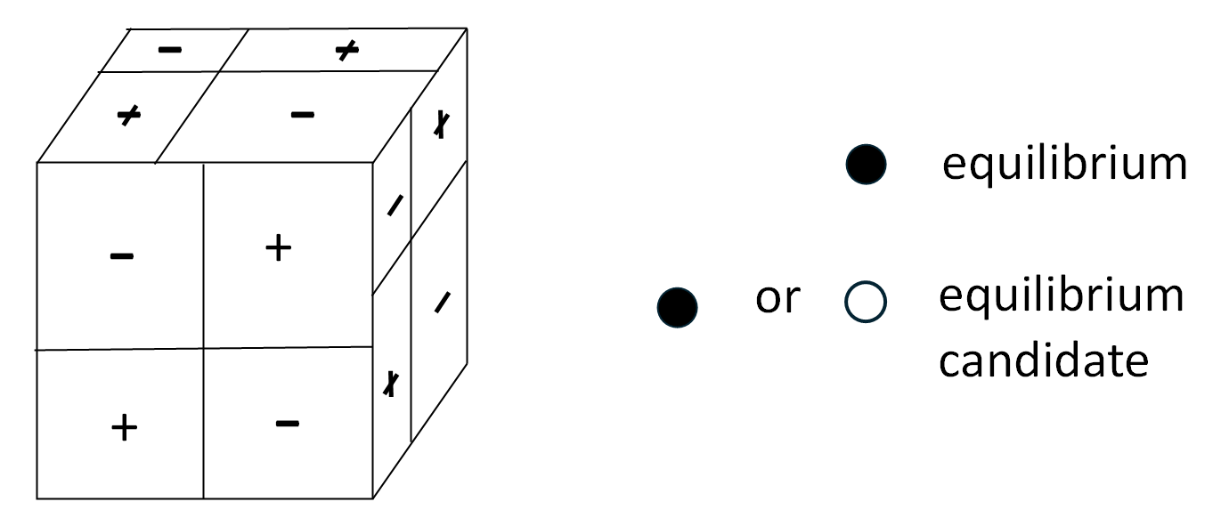
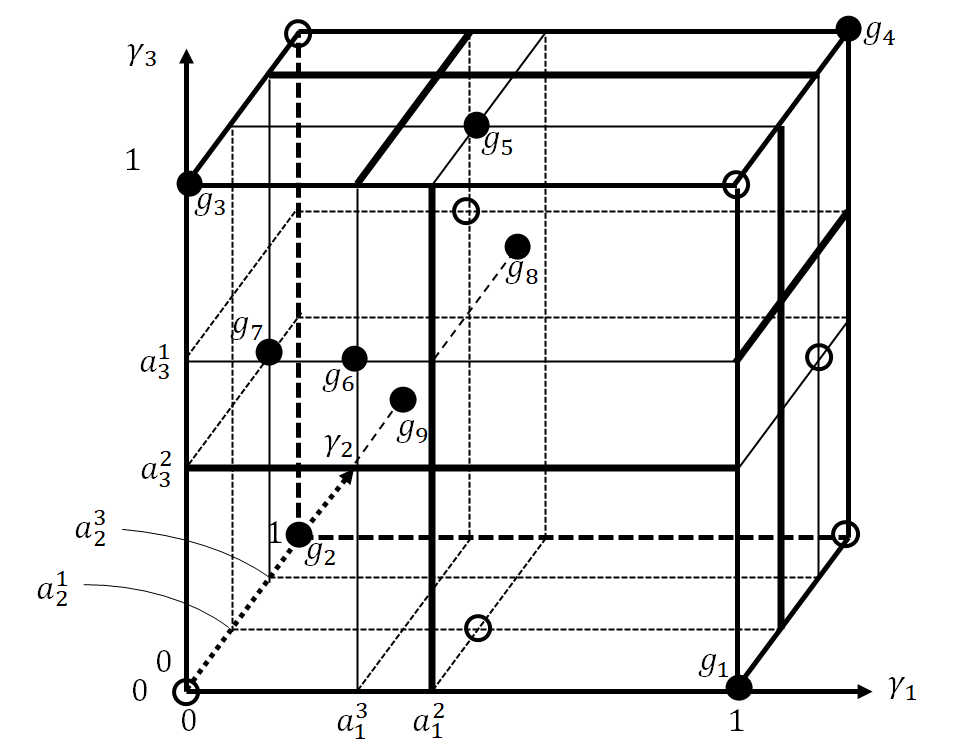
Figure 2. (iii) The upper picture shows the signs of $\lambda^{1},\lambda^{2},\lambda^{3}$. The lower picture shows the hyperplanes $\{\gamma^{j}-a^{i}_{j}=0\}\subset G\cong[0;1]^{3}$, the $8+0+6+2$ equilibrium candidates and the $4+0+3+2$ equilibria.

(iii) The right picture in Figure 1 and the picture in Figure 2 show a product two-action game with $m=3$, $\underline{v}=(v_{1},v_{2},v_{3})=(0,0,0)$ and

$$\begin{array}[]{cccc}&1>a^{2}_{1}>a^{3}_{1}>0,&1>a^{3}_{2}>a^{1}_{2}>0,&1>a^{1}_{3}>a^{2}_{3}>0,\\ \textup{so}&\sigma^{1}=\operatorname{id},&\sigma^{2}=(1\,3),&\sigma^{3}=\operatorname{id}.\end{array}$$

It has $8+0+6+2$ equilibrium candidates, namely the 8 vertices, no equilibrium candidates on the interiors of the edges, on the interior of each facet one equilibrium candidate, which is the intersection of this facet with the intersection of two walls, and two equilibrium candidates in the interior of the cube, each of which is an intersection of three walls. It has $4+0+3+2$ Nash equilibria $g^{1},...,g^{9}$, with $g^{1},g^{2},g^{3},g^{4}$ four vertices, $g^{5},g^{6},g^{7}$ on different (and not opposite) facets of the cube and $g^{8},g^{9}$ TMNE, so in the interior of the cube,

$$\begin{array}[]{lll}g^{1}\sim(1,0,0),&g^{5}\sim(a^{2}_{1},a^{1}_{2},1),&g^{8}\sim(a^{2}_{1},a^{3}_{2},a^{1}_{3}),\\ g^{2}\sim(0,1,0),&g^{6}\sim(a^{3}_{1},0,a^{1}_{3}),&g^{9}\sim(a^{3}_{1},a^{1}_{2},a^{2}_{3}),\\ g^{3}\sim(0,0,1),&g^{7}\sim(0,a^{3}_{2},a^{2}_{3}),&\\ g^{4}\sim(1,1,1).\end{array}$$

(iv) In a two-action game with $m$ players, $G\cong[0;1]^{m}$ is a hypercube. For $l\in\{0,1,...,m\}$ it has $2^{l}\begin{pmatrix}m\\ l\end{pmatrix}$ faces of dimension $m-l$. Theorem 3.7 will show that the interior of each face of dimension $m-l$ contains $!(m-l)$ equilibrium candidates, one for each derangement of the set $L^{\complement}$, where $L\subset{\mathcal{A}}$ is the set of indices $i$ of coordinates $\gamma^{i}\in\{0;1\}$ of that face. Theorem 3.7 will furthermore show the following for $l\geq 2$, for any fixed set $L$ and for any fixed derangement of $L^{\complement}$: either none of the $2^{l}$ corresponding equilibrium candidates are equilibria or half of them. Which possibility holds, depends on the characteristic tuple $(\underline{v},\underline{\sigma})$ and the derangement. For $l=0$ all equilibrium candidates are equilibria. For $l=1$ half of the equilibrium candidates are equilibria.

(v) The cube $[0;1]^{3}$ has 8 vertices, 12 edges, 6 facets and 1 interior. It has $8+0+6+2$ equilibrium candidates, just as in (iii). It has either $0+0+3+2$ equilibria or $4+0+3+2$ equilibria: The two intersection points of three walls in the interior of the cube are always equilibria. The two equilibrium candidates on opposite facets are on the same intersection line of two walls, and exactly one of them is an equilibrium. If $\underline{v}\in\{(0,0,0),(1,1,1)\}$ then 4 of the 8 vertices are equilibria, else none. All of this can be seen by looking at the figures 1 and 2. Theorem 3.7 generalizes it to arbitrary $m$.

Remarks 3.6.

(i) For arbitrary $a^{i}_{j}\in(0,1)$ with $a^{i_{1}}_{j}\neq a^{i_{2}}_{j}$ for $j\in{\mathcal{A}}$ and $i_{1}\neq i_{2}$ and an arbitrary vector $\underline{v}=(v_{1},...,v_{m})\in\{0;1\}^{m}$, a product two-action game $({\mathcal{A}},G,V)$ with polynomials $\lambda^{i}(\underline{\gamma}^{-i})$ as in (3.8) exists. For example, one can choose the multilinear map $V^{i}_{W}:W\to{\mathbb{R}}$ as

$$V^{i}_{W}(g)=\gamma^{i}_{1}\cdot(-1)^{v_{i}}\cdot\prod_{j\in{\mathcal{A}}-\{i\}}(\gamma^{j}_{1}-a^{i}_{j}(\gamma^{j}_{0}+\gamma^{j}_{1})).$$

Then $V^{i}_{W}(s^{i}_{0},g^{-i})=0$ and $V^{i}_{W}(s^{i}_{1},g^{-i})=\lambda^{i}(g^{-i})$ for $g^{-i}\in A^{-i}$.

(ii) For all product two-action games with fixed sets ${\mathcal{A}}$ and $S$, the sets of equilibrium candidates are finite and have the same structure. But the sets of equilibria depend strongly on the characteristic tuples $(\underline{v},\underline{\sigma})$. Both statements are subject of Theorem 3.7.

(iii) Product two-action games with the same characteristic tuple $(\underline{v},\underline{\sigma})$ have almost the same sets of equilibrium candidates and equilibria. The precise choice of coefficients $a^{i}_{j}\in(0;1)$ with (3.9) does not matter.

(iv) McKelvey and McLennan considered in [MM97, ch. 4] special finite games for arbitrary ${\mathcal{A}}$ and $S$ which have the maximal number of TMNE. Our product two-action games are those games in [MM97, ch. 4] which are also two-action. For them the maximal number of TMNE is $!m$. We will recover this special case of the result in [MM97, ch. 4] in Theorem 3.7 (b). But the main point of Theorem 3.7 is a simultaneous control of all equilibrium candidates and of the question which of them are Nash equilibria.

Theorem 3.7.

Let $({\mathcal{A}},G,V)$ be a product two-action game with characteristic tuple $(\underline{v},\underline{\sigma})$ and numbers $a^{i}_{j}\in(0,1)$ as in Definition 3.4.

(a) The set of equilibrium candidates (see Definition 2.3) is the set (recall Definition 3.1 (b): $L(g)=\{i\in{\mathcal{A}}\,|\,\gamma^{i}\in\{0;1\}\}$ for $g\in A$)

$$EC := \bigcup_{\pi\in S_{m}}EC(\pi)\quad\textup{with}$$ (3.12)

$$EC(\pi) := \{g\in G\,|\,L(g)=F(\pi),\ \gamma^{j}=a^{\pi(j)}_{j}\textup{ for j}\in F(\pi)^{\complement}\}.$$

We have $|EC(\pi)|=2^{|F(\pi)|}$ and $|EC|=\sum_{l=0}^{m}\begin{pmatrix}m\\ l\end{pmatrix}\cdot 2^{l}\cdot!(m-l)=V(m)$.

(b) Consider $\pi\in\operatorname{Der}_{m}$, i.e. $\pi\in S_{m}$ with $F(\pi)=\emptyset$. Then $EC(\pi)$ has only one element, and this is an equilibrium.

(c) Consider $\pi\in S_{m}$ with $F(\pi)\neq\emptyset$, and consider an equilibrium candidate $g\in EC(\pi)$. Its increment map ${\rm Inc}(g):F(\pi)\to\{0;1\}$ is defined by

$${\rm Inc}(g,i) := \Bigl{(}1+\gamma^{i}+v_{i}+|L_{0}(g)-\{i\}|\Bigr{.}$$ (3.13)

$$\Bigl{.}+\sum_{j\in F(\pi)^{\complement}}\chi(\sigma^{j}(\pi(j)),\sigma^{j}(i))\Bigr{)}\operatorname{mod}2,$$

where $\chi$ is defined by

$$\chi:{\mathbb{R}}\times{\mathbb{R}}\to\{0;1\}\textup{ with }\chi(a,b)=1\iff a\geq b.$$ (3.14)

The values ${\rm Inc}(g,i)\in\{0;1\}$ are called increments. The following holds.

• $g$ is an equilibrium if and only if ${\rm Inc}(g,i)=0$ for all $i\in F(\pi)$.

• Let $g(\pi)\in EC(\pi)$ be the equilibrium candidate in $EC(\pi)$ with $\gamma^{i}=1$ for all $i\in F(\pi)$. The map ${\rm Inc}:EC(\pi)\to\{0;1\}^{F(\pi)}$ has only two values on $EC(\pi)$, the map ${\rm Inc}(g(\pi))$ and the opposite map which takes at each $i\in F(\pi)$ the opposite value $1+Inc(g(\pi),i)\operatorname{mod}2$. The map ${\rm Inc}(g)$ coincides with the map ${\rm Inc}(g(\pi))$ if and only if $g$ and $g(\pi)$ differ in an even number of coefficients $\gamma^{i}$ for $i\in F(\pi)$ (i.e. $|L_{0}(g)|$ is even).

• Either $EC(\pi)$ contains no equilibrium or half of its elements are equilibria.

(d) Consider $\pi\in S_{m}$ with $|F(\pi)|=1$. Then $EC(\pi)$ has two elements, and one of them is an equilibrium.

(e) The only permutation $\pi$ with $|F(\pi)|=m$ is $\pi=\operatorname{id}$. In the case $\pi=\operatorname{id}$, half of the elements of $EC(\pi)$ are equilibria if and only if $\underline{v}=(0,...,0)$ or $\underline{v}=(1,...,1)$.

(f) There is no permutation $\pi\in S_{m}$ with $|F(\pi)|=m-1$.

Proof: (a) Let $g\in G$ be an equilibrium candidate. Recall $L_{0}(g),L_{1}(g)$ and $L(g)=L_{0}(g)\cup L_{1}(g)$ from Definition 3.1 (b). For $i\in L_{0}(g)$ $\gamma^{i}=0$. For $i\in L_{1}(g)$ $\gamma^{i}=1$. For $i\in L(g)^{\complement}$ we have $0\in{\rm supp}(g)$ and $1\in{\rm supp}(g)$ and therefore by condition 2.3

$$0=\lambda^{i}(\underline{\gamma}^{-i})=(-1)^{v_{i}}\prod_{j\in{\mathcal{A}}-\{i\}}(\gamma^{j}-a^{i}_{j}).$$

Therefore there is a map

$$\widetilde{\pi}:{\mathcal{A}}\to{\mathcal{A}} \textup{ with }\widetilde{\pi}(i)=i\textup{ for }i\in L(g),$$

$$\textup{and with }\widetilde{\pi}(i)\neq i\textup{ and }\gamma^{\widetilde{\pi}(i)}=a^{i}_{\widetilde{\pi}(i)}\textup{ for }i\in L(g)^{\complement}.$$

Because for each $j\in{\mathcal{A}}$ the coefficients $a^{i}_{j}$ for $i\in{\mathcal{A}}-\{j\}$ are pairwise different and not in $\{0;1\}$, the map $\widetilde{\pi}$ is a permutation with $F(\widetilde{\pi})=L(g)$, and it is unique. Write $\pi:=\widetilde{\pi}^{-1}$. Also $\pi$ is a permutation with $F(\pi)=L(g)$. Therefore the condition $\gamma^{\widetilde{\pi}(i)}=a^{i}_{\widetilde{\pi}(i)}$ for $i\in L(g)^{\complement}$ can also be written as

$$\gamma^{j}=a^{\pi(j)}_{j}\quad\textup{for}\quad j\in F(\pi)^{\complement}.$$ (3.15)

Vice versa, for any permutation $\pi\in S_{m}$, the element $g$ with (3.15) and $g^{i}\in\{0;1\}$ for $i\in F(\pi)$ is an equilibrium candidate. Obviously $|EC(\pi)|=2^{|F(\pi)|}$. The number of subsets $L\subset{\mathcal{A}}$ with $|L|=l$ is $\begin{pmatrix}m\\ l\end{pmatrix}$. The number of derangements on a set $L^{\complement}$ with $|L|=l$ is $!(m-l)$. Therefore $|EC|$ is as claimed.

(b) In the case $\pi\in Der_{m}$, the set $EC(\pi)$ has only one element which is now called $g$. All its coefficients $\gamma^{i}$ are in $(0;1)$, so ${\rm supp}(g)=J$ is maximal. Therefore in Remark 2.2, the condition (2.4) is empty, so the conditions for an equilibrium and for an equilibrium candidate coincide. Therefore $g$ is an equilibrium.

(c) Now consider $\pi\in S_{m}$ with $F(\pi)\neq\emptyset$. An equilibrium candidate $g\in EC(\pi)$ is by Remark 2.2 an equilibrium if $\lambda^{i}(\underline{\gamma}^{-i})\geq 0$ for $\gamma^{i}=1$ and $\lambda^{i}(\underline{\gamma}^{-i})\leq 0$ for $\gamma^{i}=0$. But $\lambda^{i}(\underline{\gamma}^{-i})\in{\mathbb{R}}^{*}$ for $i\in F(\pi)=L(g)$ because it is

$$\lambda^{i}(\underline{\gamma}^{-i})=(-1)^{v_{i}}\prod_{j\in{\mathcal{A}}-\{i\}}(\gamma^{j}-a^{i}_{j})=$$

$$(-1)^{v_{i}}\Bigl{(}\prod_{j\in L_{1}(g)-\{i\}}(1-a^{i}_{j})\Bigr{)}\Bigl{(}\prod_{j\in L_{0}(g)-\{i\}}(0-a^{i}_{j})\Bigr{)}\Bigl{(}\prod_{j\in F(\pi)^{\complement}}(a^{\pi(j)}_{j}-a^{i}_{j})\Bigr{)},$$

and all $a^{i}_{j}\in(0,1)$, and furthermore $a^{\pi(j)}_{j}\neq a^{i}_{j}$ for $j\in F(\pi)^{\complement}$ because $\pi(j)\in F(\pi)^{\complement}$ and $i\in F(\pi)$. Therefore $g\in EC(\pi)$ is an equilibrium if and only if $\operatorname{sign}(\lambda^{i}(\underline{\gamma}^{-i}))=(-1)^{1+\gamma^{i}}$ for any $i\in F(\pi)$.

The sign of $\lambda^{i}(\underline{\gamma}^{-i})$ is

$$\operatorname{sign}(\lambda^{i}(\underline{\gamma}^{-i})) = (-1)^{v_{i}}(-1)^{|L_{0}(g)-\{i\}|}\cdot\prod_{j\in F(\pi)^{\complement}}\operatorname{sign}\bigl{(}a^{\pi(j)}_{j}-a^{i}_{j}\bigr{)}$$

$$= (-1)^{v_{i}}(-1)^{|L_{0}(g)-\{i\}|}\cdot\prod_{j\in F(\pi)^{\complement}}(-1)^{\chi(\sigma^{j}(\pi(j)),\sigma^{j}(i))}.$$

Here $\operatorname{sign}\bigl{(}a^{\pi(j)}_{j}-a^{i}_{j}\bigr{)}=(-1)^{\chi(\sigma^{j}(\pi(j)),\sigma^{j}(i))}$ because of (3.9) (and (3.14)). The condition $\operatorname{sign}(\lambda^{i}(\underline{\gamma}^{-i}))=(-1)^{1+\gamma^{i}}$ for $i\in F(\pi)$ is equivalent to the condition ${\rm Inc}(g,i)=0$. This proves part (i).

For part (ii), consider an equilibrium candidate $\widetilde{g}\in EC(\pi)$ which differs from $g$ only in one coordinate, so $\widetilde{\gamma}^{j}=\gamma^{j}=a^{\pi(j)}_{j}$ for $j\in F(\pi)^{\complement}$, $\widetilde{\gamma}^{i}=\gamma^{i}$ for $i\in F(\pi)-\{i_{0}\}$ for one $i_{0}\in F(\pi)$, and $\widetilde{\gamma}^{i_{0}}\equiv 1+\gamma^{i_{0}}\operatorname{mod}2$. Only the part

$$\bigl{(}\gamma^{i}+|L_{0}(g)-\{i\}|\bigr{)}\operatorname{mod}2$$

of ${\rm Inc}(g,i)$ depends on $g$. For $i\in F(\pi)-\{i_{0}\}$, we have $\widetilde{\gamma}^{i}=\gamma^{i}$ and $|L_{0}(\widetilde{g})-\{i\}|\equiv 1+|L_{0}(g)-\{i\}|\operatorname{mod}2$, so ${\rm Inc}(\widetilde{g},i)\equiv 1+{\rm Inc}(g,i)\operatorname{mod}2$. For $i=i_{0}$, we have $\widetilde{\gamma}^{i}\equiv 1+\gamma^{i}\operatorname{mod}2$ and $|L_{0}(\widetilde{g})-\{i\}|\equiv|L_{0}(g)-\{i\}|\operatorname{mod}2$, so ${\rm Inc}(\widetilde{g},i)\equiv 1+{\rm Inc}(g,i)\operatorname{mod}2$. This proves part (ii).

Part (iii) follows immediately from the parts (i) and (ii).

(d) Suppose $F(\pi)=\{i_{0}\}$. Here $EC(\pi)$ consists only of $g(\pi)$ and one other equilibrium candidate $g_{2}$. By (c)(ii) ${\rm Inc}(g_{2},i_{0})=1+{\rm Inc}(g(\pi),i_{0})\operatorname{mod}2$, so by (c)(i) exactly one of them is an equilibrium.

(e) In the case $\pi=\operatorname{id}$, we have $F(\pi)^{\complement}=\emptyset$ and ${\rm Inc}(g(\pi),i)\equiv 1+1+v_{i}+0\equiv v_{i}\operatorname{mod}2$. So $g(\pi)$ is an equilibrium if and only if $\underline{v}=(0,...,0)$, and an equilibrium candidate in $EC(\pi)$ which differs in an odd number of coefficients from $g(\pi)$ is an equilibrium if and only if $\underline{v}=(1,...,1)$.

(f) This follows from $!1=0$ or $\operatorname{Der}_{1}=\emptyset$. $\Box$

4. Maximal product two-action games

This section proves the main result of the paper, the existence of generic two-action games with $\frac{1}{2}(V(m)+!m)$ Nash equilibria. The main point is to find product two-action games with so many Nash equilibria.

Recall that Theorem 3.7 (c) implies for a product two-action game $({\mathcal{A}},G,V)$ and a permutation $\pi\in S_{m}-\operatorname{Der}_{m}$ the following: Either half of the equilibrium candidates in $EC(\pi)$ are equilibria or none of them are equilibria. The first case holds if and only if ${\rm Inc}(g(\pi)):F(\pi)\to\{0;1\}$ has either only value 0 or only value 1.

Definition 4.1.

A product two-action game $({\mathcal{A}},G,V)$ is maximal if for any permutation $\pi\in S_{m}-\textup{Der}_{m}$ half of the equilibrium candidates in $EC(\pi)$ are equilibria.

The main result of this paper is that for any number $m\in{\mathbb{N}}$, maximal product two-action games exists. The point is to find a suitable characteristic tuple $(\underline{v},\underline{\sigma})$. The way, how we found it, was by a systematic analysis of the cases with small $m$, via a system of linear equations which gives the increment maps in terms of tuples of numbers associated to the characteristic tuple $(\underline{v},\underline{\sigma})$. Here we will not describe this system of linear equations, but give the characteristic tuple $(\underline{v},\underline{\sigma})$ of certain product two-action games and then show that these games are maximal. The permutations $\delta^{i}$ in the next lemma are part of the characteristic tuple. The lemma itself is trivial.

Lemma 4.2.

Fix $m\in{\mathbb{N}}$ and ${\mathcal{A}}=\{1,...,m\}$. For $i\in{\mathcal{A}}$ define the following three permutations $\alpha^{i},\beta^{i}$ and $\delta^{i}\in S_{m}$. (Recall the definition of $\chi:{\mathbb{R}}\times{\mathbb{R}}\to\{0;1\}$ in (3.14)).

$$\alpha^{i} := \left(\begin{array}[]{lllll}j&\mapsto&j&\textup{if}&1\leq j\leq i-1,\\ i&\mapsto&m&&\\ j&\mapsto&j-1&\textup{if}&i+1\leq j\leq m.\end{array}\right)$$

$$= \begin{pmatrix}1&...&i-1&i&i+1&...&m\\ 1&...&i-1&m&i&...&m-1\end{pmatrix}=(m\ m-1\ ...\ i+1\ i),$$

$$\beta^{i} := \left(\begin{array}[]{lllll}j&\mapsto&m-i+j&\textup{if}&1\leq j\leq i-1,\\ j&\mapsto&j-i+1&\textup{if}&i\leq j\leq m-1,\\ m&\mapsto&m&&\end{array}\right)$$

$$= \begin{pmatrix}1&...&i-1&i&...&m-1&m\\ m-i+1&...&m-1&1&...&m-i&m\end{pmatrix},$$

$$\delta^{i} := (\alpha^{i})^{-1}\circ\beta^{i}\circ\alpha^{i}.$$

$\delta^{i}$ is the permutation

$$\delta^{i}=\left(\begin{array}[]{lllll}j&\mapsto&m-i+j+\chi(m-i+j,i)&\textup{if}&1\leq j\leq i-1,\\ i&\mapsto&i&&\\ j&\mapsto&j-i+\chi(j-i,i)&\textup{if}&i+1\leq j\leq m.\end{array}\right).$$

$\delta^{i}$ is the unique permutation in $S_{m}$ with $\delta^{i}(i)=i$ and with the following property: $\delta^{i}(j_{1})>\delta^{i}(j_{2})$ for $j_{1},j_{2}\in{\mathcal{A}}-\{i\}$ with $j_{1}<j_{2}$ if and only if $j_{1}\in\{1,...,i-1\}$ and $j_{2}\in\{i+1,...,m\}$.

Example 4.3.

In the case $m=3$

$$\delta^{1}=\operatorname{id},\ \delta^{2}=(1\,3)=\begin{pmatrix}1&2&3\\ 3&2&1\end{pmatrix},\ \delta^{3}=\operatorname{id}.$$

The product two-action game with $m=3$ in Example 3.4 has the characteristic pair $(\underline{v},\underline{\sigma})=((0,0,0),(\delta^{1},\delta^{2},\delta^{3}))$. It has $4+0+3+2=9$ Nash equilibria, so it is a maximal product two-action game.

Theorem 4.4.

Fix $m\in{\mathbb{N}}$ and ${\mathcal{A}}=\{1,....,m\}$. Any product two-action game with the characteristic tuple $(\underline{v},\underline{\sigma})=((0,...,0),(\delta^{1},...,\delta^{m}))$ is maximal.

Proof: Consider a product two-action game with the characteristic tuple $(\underline{v},\underline{\sigma})=((0,...,0),(\delta^{1},...,\delta^{m}))$. Fix a permutation $\pi\in S_{m}-\operatorname{Der}_{m}$. Recall that $g(\pi)\in EC(\pi)$ is the equilibrium candidate with $\gamma^{i}=1$ for each $i\in F(\pi)$ (Theorem 3.7 (c)(ii)). Because of Corollary 3.7, it is sufficient to show that the increment map ${\rm Inc}(g(\pi))\in\{0,1\}^{F(\pi)}$ has either only value 0 or only value 1. Because $g(\pi)$ satisfies $L_{0}(g(\pi))=\emptyset$ and $\gamma^{i}=1$ for $i\in F(\pi)$, we have

$${\rm Inc}(g(\pi),i)\equiv\Bigl{(}\sum_{j\in F(\pi)^{\complement}}\chi(\delta^{j}(\pi(j)),\delta^{j}(i))\Bigr{)}\operatorname{mod}2\quad\textup{for}\quad i\in F(\pi).$$

Claim: For $i\in F(\pi)$ and $j\in F(\pi)^{\complement}$

$$\chi(\delta^{j}(\pi(j)),\delta^{j}(i))=\left\{\begin{array}[]{ll}1&\textup{if }j<i\textup{ and }(\pi(j)<j\textup{ or }\pi(j)>i),\\ 0&\textup{if }j<i\textup{ and }j<\pi(j)<i,\\ 0&\textup{if }j>i\textup{ and }(\pi(j)<i\textup{ or }\pi(j)>j),\\ 1&\textup{if }j>i\textup{ and }i<\pi(j)<j.\end{array}\right.$$ (4.8)

Proof of Claim (4.8): Recall that $\chi(\delta^{j}(\pi(j)),\delta^{j}(i))=1$ if and only if $\delta^{j}(\pi(j))>\delta^{j}(i)$. Recall the characterization of $\delta^{j}$ at the end of Lemma 4.2.

First consider the case $j\in F(\pi)^{\complement}$ with $j<i$. If $\pi(j)>i$ then also $\delta^{j}(\pi(j))>\delta^{j}(i)$. If $\pi(j)\in\{j+1,...,i-1\}$ then $j<\pi(j)<i$ and also $\delta^{j}(\pi(j))<\delta^{j}(i)$. If $\pi(j)<j$ then $\delta^{j}(\pi(j))>\delta^{j}(i)$.

Now consider the case $j\in F(\pi)^{\complement}$ with $j>i$. If $\pi(j)>j$ then $\delta^{j}(\pi(j))<\delta^{j}(i)$. If $\pi(j)\in\{i+1,...,j-1\}$ then $j>\pi(j)>i$ and also $\delta^{j}(\pi(j))>\delta^{j}(i)$. If $\pi(j)<i$ then also $\delta^{j}(\pi(j))<\delta^{j}(i)$. This finishes the proof of Claim (4.8). $(\Box)$

If $|F(\pi)|=1$, nothing has to be shown as then the definition domain $F(\pi)$ of ${\rm Inc}(g(\pi))$ has only one element. So suppose $|F(\pi)|\geq 2$, and fix two elements $i_{1},i_{2}\in F(\pi)$ with $i_{1}<i_{2}$.

Claim (4.8) shows which $j\in F(\pi)^{\complement}$ give the same contributions to ${\rm Inc}(g(\pi),i_{1})$ and to ${\rm Inc}(g(\pi),i_{2})$, and which give different contributions. The splitting into the following 9 cases is natural. In the following table, $\chi(\delta^{j}(\pi(j),\delta^{j}(i_{1}))$ and $\chi(\delta^{j}(\pi(j),\delta^{j}(i_{2}))$ are abbreviated as $\chi[i_{1}]$ and $\chi[i_{2}]$.

$$\begin{array}[]{l|l|l|l|l}Case&&&\chi[i_{1}]&\chi[i_{2}]\\ \hline\cr(1)&j<i_{1}&\pi(j)<j\textup{ or }\pi(j)>i_{2}&1&1\\ (2)&j<i_{1}&j<\pi(j)<i_{1}&0&0\\ (3)&j<i_{1}&i_{1}<\pi(j)<i_{2}&1&0\\ (4)&j>i_{2}&\pi(j)<i_{1}\textup{ or }\pi(j)>j&0&0\\ (5)&j>i_{2}&i_{2}<\pi(j)<j&1&1\\ (6)&j>i_{2}&i_{1}<\pi(j)<i_{2}&1&0\\ (7)&i_{1}<j<i_{2}&i_{1}<\pi(j)<j&1&1\\ (8)&i_{1}<j<i_{2}&j<\pi(j)<i_{2}&0&0\\ (9)&i_{1}<j<i_{2}&\pi(j)<i_{1}\textup{ or }\pi(j)>i_{2}&0&1\end{array}$$

Only the cases (3), (6) and (9) give different contributions to ${\rm Inc}(g(\pi),i_{1})$ and to ${\rm Inc}(g(\pi),i_{2})$. The number of the $j$ in the cases (3) and (6) together is the same as the number of the $j$ in the case (9), as $\pi$ is a bijection. Therefore the number of different contributions is even. This shows ${\rm Inc}(g(\pi),i_{1})={\rm Inc}(g(\pi),i_{2})$. Therefore the increment map ${\rm Inc}(g(\pi))$ has either only value 0 or only value 1. This finishes the proof of Theorem 4.4. $\Box$

Corollary 4.5.

(a) A maximal product two-action game has $\frac{1}{2}(V(m)+!m)$ Nash equilibria.

(b) A small generic deformation of a product two-action game has the same number of Nash equilibria as the product two-action game.

(c) The inequality (1.5) $\frac{1}{2}(V(m)+!m)\leq\mu(m;2,...,2)$ holds.

Proof: (a) In a maximal product two-action game, the number of Nash equilibria is

$$\sum_{\pi\in\operatorname{Der}_{m}}1+\sum_{\pi\in S_{m}-\operatorname{Der}_{m}}\frac{1}{2}|EC(\pi)|=\frac{1}{2}!m+\frac{1}{2}\sum_{\pi\in S_{m}}|EC(\pi)|=\frac{1}{2}(!m+V(m)).$$

(b) An equilibrium candidate $g\in EC(\pi)$ of a product two-action game satisfies $L_{0}(g)\dot{\cup}L_{1}(g)=L(g)=F(\pi)$, and it is an intersection point of the zero hypersurfaces of the functions in the following tuple of functions,

$$\Bigl{(}\gamma^{i}\,|\,i\in L_{0}(g);\quad\gamma^{i}-1\,|\,i\in L_{1}(g);\quad\lambda^{i}(\underline{\gamma}^{-i})\,|\,i\in F(\pi)^{\complement}\Bigr{)}.$$ (4.10)

Locally near $g$, these zero hypersurfaces coincide with the zero hypersurfaces of the functions in the following tuple,

$$\Bigl{(}\gamma^{i}\,|\,i\in L_{0}(g);\quad\gamma^{i}-1\,|\,i\in L_{1}(g);\quad\gamma^{i}-a_{i}^{\pi(i)}\,|\,i\in F(\pi)^{\complement}\Bigr{)}.$$ (4.11)

Obviously locally near $g$, these zero hypersurfaces are smooth and transversal (therefore $g$ may be called a regular equilibrium candidate, see e.g. [Ha73]). This property is preserved for the zero hypersurfaces in the tuple in (4.10) by a small deformation of the product two-action game to a generic two-action game. Therefore $g$ deforms to an equilibrium candidate of the deformed game.

If $g$ is a Nash equilibrium, it satisfies additionally the inequalities

$$\lambda^{i}(\underline{\gamma}^{-i}) < 0\quad\textup{for }i\in L_{0}(g),$$

$$\lambda^{i}(\underline{\gamma}^{-i}) > 0\quad\textup{for }i\in L_{1}(g).$$

Also these inequalities are preserved by a small generic deformation. Therefore a Nash equilibrium deforms to a Nash equilibrium.

(c) One considers a small generic deformation of a maximal product two-action game and applies (a) and (b). $\Box$

5. A conjecture

Consider a two-action game $({\mathcal{A}},G,V)$. The hypercube $G\cong[0;1]^{m}$ is the disjoint union $\dot{\bigcup}_{l=0}^{m}C_{l}$ of the following subsets

$$C_{l}:=\{g\in G\,|\,|L(g)|=l\}=\{g\in G\,|\,|\{i\in{\mathcal{A}}\,|\ \gamma^{i}\in\{0;1\}\}|=l\}.$$

$C_{l}$ is the union of the open faces of dimension $n-l$ of the hypercube $G$ as a polytope.

Lemma 5.1.

(a) In the case of a generic two-action game

$$|{\mathcal{N}}\cap C_{0}| \leq !m,$$ (5.1)

$$|{\mathcal{N}}\cap C_{m-1}| = 0,$$ (5.2)

$$|{\mathcal{N}}\cap C_{m}| \leq 2^{m-1}.$$ (5.3)

(b) In the case of a product two-action game or a generic two-action game which is close to a product two-action game

$$|{\mathcal{N}}\cap C_{0}| = !m,$$ (5.4)

$$|{\mathcal{N}}\cap C_{l}| \leq \begin{pmatrix}m\\ l\end{pmatrix}\cdot 2^{l-1}\cdot!(m-l)\quad\textup{for }l\geq 1.$$ (5.5)

In the case of a maximal product two-action game, the inequalities in (5.5) are binding, i.e. they are equalities.

Proof: (a) (5.1) is the upper bound of McKelvey and McLennan [MM97] for TMNE in the case of generic two-action games.

In a generic two-action game, the best reply set $r^{i}(s^{-i})\subset G^{i}$ of any pure strategy combination $s^{-i}\in S^{-i}$ is either $\{s^{i}_{0}\}$ or $\{s^{i}_{1}\}$. This implies ${\mathcal{N}}\cap C_{m-1}=\emptyset$, so (5.2). It also shows that $(s^{i}_{0},s^{-i})$ and $(s^{i}_{1},s^{-i})$ cannot both be equilibria. So, of two neighboring vertices of $G$ only one can be an equilibrium. Therefore at most $2^{m-1}$ of the $2^{m}$ vertices of $G$ can be Nash equilibria.

(b) For product two-action games, (5.4) and (5.5) follow from Theorem 3.7. For generic two-action games which are close to product two-action games, (5.4) and (5.5) follow from Theorem 3.7 and the proof of Corollary 4.5. $\Box$

(5.2) and (5.3) coincide with (5.5) for $l\in\{m-1,m\}$. But for $l\in\{1,2,...,m-2\}$, (5.5) does not necessarily hold for arbitrary generic two-action games. Our observation from special cases is that in a not so small deformation of a product two-action game, the $C_{l}$-type of an equilibrium may change.

We conjecture (optimistically) that the maximal number of Nash equilibria in product two-action games is also the maximal number in all generic two-action games, so $\mu(m;2,...,2)\stackrel{{\scriptstyle?}}{{=}}\frac{1}{2}(V(m)+!m)$. We even conjecture the following stronger semicontinuity property for the possible $C_{l}$-types of Nash equilibria in generic two-action games.

Conjecture 5.2.

Let $({\mathcal{A}},G,V)$ be a generic two-action game. Then for each $d\in\{0,1,...,m\}$

$$\sum_{l=0}^{d}|{\mathcal{N}}\cap C_{l}|\leq!m+\sum_{l=1}^{d}\begin{pmatrix}m\\ l\end{pmatrix}\cdot 2^{l-1}\cdot!(m-l).$$ (5.6)

The case $d=m$ is the conjecture $\mu(m;2,...,2)\stackrel{{\scriptstyle?}}{{=}}\frac{1}{2}(V(m)+!m)$.

In the case $m=3$ this conjecture was recently proved by Jahani and von Stengel.

Theorem 5.3.

[JS24] Conjecture 5.2 is true in the case $m=3$. Explicitly: Any generic two-action game with $m=3$ satisfies

$$|{\mathcal{N}}\cap C_{0}| \leq 2,$$ (5.7)

$$|{\mathcal{N}}\cap C_{0}|+|{\mathcal{N}}\cap C_{1}| \leq 2+3=5,$$ (5.8)

$$|{\mathcal{N}}\cap C_{0}|+|{\mathcal{N}}\cap C_{1}|+|{\mathcal{N}}\cap C_{2}| \leq 2+3+0=5,$$ (5.9)

$$\sum_{l=0}^{3}|{\mathcal{N}}\cap C_{l}|=|{\mathcal{N}}| \leq 2+3+0+4=9$$

$$= \mu(3;2,2,2)=\frac{1}{2}(V(3)+!3).$$

The inequality (5.7) is a special case of the result in [MM97] on TMNE. The inequality (5.3) is the main result in [JS24]. The inequality (5.9) follows from (5.8) and $|{\mathcal{N}}\cap C_{2}|=0$. It remains to see how the results in [JS24] imply the inequality (5.8).

Theorem 8 in Chapter 3 in [JS24] shows $|{\mathcal{N}}\cap C_{0}|=2\Longrightarrow|{\mathcal{N}}\cap C_{1}|\leq 3$. Chapter 4 in [JS24] treats the cases with $|{\mathcal{N}}\cap C_{0}|\leq 1$. An index argument shows in these cases

$$|{\mathcal{N}}\cap C_{3}|-|{\mathcal{N}}\cap C_{1}|+\varepsilon|{\mathcal{N}}\cap C_{0}|=1\quad\textup{for some }\varepsilon\in\{\pm 1\}.$$

This and $|{\mathcal{N}}\cap C_{3}|\leq 4$ imply in these cases $|{\mathcal{N}}\cap C_{0}|+|{\mathcal{N}}\cap C_{1}|\leq 5$.

Remarks 5.4.

(i) The inequality $|{\mathcal{N}}|\leq 9$ for a generic two-action game with $m=3$ is also claimed in [Vi17, Remark 5.6], but without proof.

(ii) The case of a two-action game with $m=3$ is also considered in the following three papers.

Chin, Parthasarathy and Raghavan [CPR73, Theorem 6] prove for each two-action game with $m=3$ and with ${\mathcal{N}}\subset\textup{interior}(G)$ that $|{\mathcal{N}}|=1$. For generic games this follows from the upper bound $2$ for the number of TMNE and from the oddness of $|{\mathcal{N}}|$. But they proved it for each two-action game with $m=3$.

McKelvey and McLennan [MM97, ch. 6] reprove in an explicit way their upper bound $!3=2$ for the number of TMNE in a generic two-action game with $m=3$.

Jahani and von Stengel [JS22] present an algorithmic approach to finding all Nash equilibria of any two-action game with $m=3$.

References

[CPR73] H. Chin, T. Parthasarathy, T.E.S.
Raghavan: Structure of equilibria in -person
non-cooperative games.
Int. J. Game Theory 3 (1973), 1–19.
[Ha73] J.C. Harsanyi: Oddness of the number of equilibrium points: A new proof.
Int. J. Game Theory 2 (1973), 235–250.
[JS22] S. Jahani, B. von Stengel: Automated equilibrium analysis of
games.
In: Kanellopoulos, P., Kyropoulou, M., Voudouris, A. (eds)
Algorithmic Game Theory. SAGT 2022.
Lecture Notes in Computer Science, vol. 13584, pp
223-237. Springer, Cham.
[JS24] S. Jahani, B. von Stengel: Generic three-player two-action games have at most
nine Nash equilibria. Preprint, 10 pages, April 2024.
[Ke97] H. Keiding: On the maximal number of Nash equilibria in an
bimatrix game.
Games Econom. Behav. 21 (1997), 148–160.
[MM97] R.D. McKelvey, A. McLennan: The maximal number of regular totally mixed Nash
equilibria.
J. Econom. Theory 72.2 (1997), 411–425.
[MP99] A. McLennan, I.-U. Park: Generic two person games have at most 15
Nash equilibria.
Games Econom. Behav. 26.1 (1999), 111–130.
[Na51] J.F. Nash: Non-cooperative games.
Ann. of Math. 54 (1951), 286–295.
[QS97] T. Quint, M. Shubik: A theorem on the number of Nash equilibria in a
bimatrix game.
Int. J. Game Theory 26 (1997), 353–360.
[Ro71] J. Rosenmüller: On a generalization of the Lemke-Howson algorithm to
noncooperative -person games.
SIAM J. Appl. Math. 21.1 (1971), 73–79.
[St97] B. von Stengel: New lower bounds for the number of equilibria in bimatrix
games.
Technical Report 264, Dept. of Computer Science, ETH Zürich,
1997.
[St99] B. von Stengel: New maximal numbers of equilibria in bimatrix games.
Discrete Comput. Geom. 21.4 (1999), 557–568.
[Vi17] R. Vidunas: Counting derangements and Nash equilibria.
Ann. Com. 21 (2017), 131–152.
[Wi71] R. Wilson: Computing equilibria of -person games.
SIAM J. Appl. Math. 21.1 (1971), 80–87.