Stability Bounds for the Unfolded Forward-Backward Algorithm

Abstract

We consider a neural network architecture designed to solve inverse problems where the degradation operator is linear and known. This architecture is constructed by unrolling a forward-backward algorithm derived from the minimization of an objective function that combines a data-fidelity term, a Tikhonov-type regularization term, and a potentially nonsmooth convex penalty. The robustness of this inversion method to input perturbations is analyzed theoretically. Ensuring robustness complies with the principles of inverse problem theory, as it ensures both the continuity of the inversion method and the resilience to small noise - a critical property given the known vulnerability of deep neural networks to adversarial perturbations. A key novelty of our work lies in examining the robustness of the proposed network to perturbations in its bias, which represents the observed data in the inverse problem. Additionally, we provide numerical illustrations of the analytical Lipschitz bounds derived in our analysis.

1 Introduction

Inverse problems

A large variety of inverse problems consists of inverting convolution operators such as signal/image restoration [1, 2], tomography [3], Fredholm equation of the first kind [4], or inverse Laplace transform [5].

Let $T$ be a bounded linear operator from a separable Hilbert space $\mathscr{X}$ to a Hilbert space $\mathscr{Y}$. The problem consists in finding $x\in\mathscr{X}$ from observed data

$$y=Tx+w$$ (1)

where $w$ corresponds to an additive measurement noise. The above problem is often ill-posed i.e., a solution might not exist, might not be unique, or might not depend continuously on the data.

Variational problem

The well-posedness of the inverse problem defined by (1) is retrieved by regularization. Here we consider Tikhonov-type regularization. Let $\tau\in]0,+\infty[$ be the regularization parameter. Solving the inverse problem (1) with such regularization, leads to the resolution of the following optimization problem:

$$\underset{x\in C}{\text{minimize}}\,J_{\tau}(x)\;,$$ (2)

where

$$(\forall x\in\mathscr{X})\quad J_{\tau}(x)=\frac{1}{2}\|Tx-y\|^{2}+\frac{\tau}{2}\|Dx\|^{2},$$ (3)

$C$ is a nonempty closed convex subset of $\mathscr{X}$ encoding some prior knowledge, e.g. some range constraint or sparsity pattern, while $D$ acts as a derivative operator of some order $r\geq 0$. Often, we have an a priori of smoothness on the solution which justifies the use of such a derivative-based regularization. Problem (2) is actually an instance of the more general class of problems stated below, encountered in many signal/image processing tasks:

$$\underset{x\in\mathscr{X}}{\text{minimize}}\,J_{\tau}(x)+\mu\,g(x)\;,$$ (4)

where $\mu\in[0,+\infty[$ is an additional regularization constant and $g$ is a proper lower-semicontinuous convex function from Hilbert space $\mathscr{X}$ to $]-\infty,+\infty]$. Indeed, Problem (2) corresponds to the case when $g$ is the indicator function $\iota_{C}$ of set $C$.

Neural network

We focus our attention on seeking for a solution to the addressed inverse problem through nonlinear approximation techniques making use of neural networks. Thus, instead of considering the solution to the regularized problem (4), we define the solution to the inverse problem (1) as the output of a neural network, whose structure is similar to a recurrent network [6, 7].

Namely, by setting an initial value $x_{0}$, we are interested in the following $m$-layers neural network where $m\in\mathbb{N}\setminus\{0\}$:

$$\begin{cases}\textbf{Initialization:}\\ \quad b_{0}=T^{*}y,\\ \textbf{Layer $n\in\{1,\ldots,m\}$:}\\ \quad x_{n}=\text{prox}_{\lambda_{n}\mu_{n}g}\big{(}x_{n-1}-\lambda_{n}(T^{*}T+D_{n}^{*}D_{n})x_{n-1}+\lambda_{n}b_{0}\big{)}\;.\end{cases}$$ (5)

Hereabove, $\text{prox}_{\varphi}$ stands for the proximity operator of a lower-semicontinuous proper convex function $\varphi$ (see Section 2) and, for every $n\in\{1,\ldots,m\}$, $D_{n}$ is a bounded linear operators from $\mathscr{X}$ to some Hilbert space $\mathscr{Z}$, and $\lambda_{n}$ is positive real. Throughout this paper, $L^{*}$ denotes the adjoint of a bounded linear operator $L$ defined on suitable Hilbert spaces. The overall structure of the network is shown in Figure 1.

Figure 1: Global architecture of the $m$-layers neural network (5).

A simple choice consists in setting, for every $n\in\{1,\ldots,m\}$, $D_{n}=\sqrt{\tau_{n}}D$ where $\tau_{n}$ is a positive constant. The constants $(\mu_{n})_{1\leq n\leq m}$, $(\tau_{n})_{1\leq n\leq m}$, and possibly $(\lambda_{n})_{1\leq n\leq m}$ can be learned during training. Then, Model (6) can be viewed as unrolling $m$ iterations of an optimization algorithm, so leading to Algorithm 1. If additionally, we set $\mu_{n}\equiv\mu$ and $\tau_{n}\equiv\tau$, Algorithm 1 identifies with the forward-backward algorithm [8, 9] applied to the variational problem (4).

Algorithm 1 Proximal forward-backward splitting method

1:Set $x_{0}$ ,

2:for $n=1,2,\ldots,m$ do

3:  Set $\lambda_{n},\tau_{n},\mu_{n}$ ,

4:  $x_{n}=\text{prox}_{\lambda_{n}\mu_{n}g}\;\left(x_{n-1}-\lambda_{n}\nabla J_{\tau_{n}}(x_{n-1})\right)$ ,

5:end for

6:return $x_{m}$

Let $\overline{\chi}\geq 0$ denote the modulus of strong convexity of the regularization term $g$ (with $\overline{\chi}>0$ if $g$ is strongly convex). We have thus $g=g_{0}+\overline{\chi}\|\cdot\|^{2}/2$ where $g_{0}$ is a proper lower-semicontinuous convex function from $\mathscr{X}$ to $]-\infty,+\infty]$, and Model (5) can be equivalently expressed as

$$\begin{cases}\textbf{Initialization:}\\ \quad b_{0}=T^{*}y,\\ \textbf{Layer $n\in\{1,\ldots,m\}$:}\\ \quad x_{n}=R_{n}(W_{n}x_{n-1}+V_{n}b_{0})\;,\end{cases}$$ (6)

where, for every $n\in\{1,\ldots,m\}$,

$$R_{n}=\text{prox}_{\frac{\lambda_{n}\mu_{n}}{1+\lambda_{n}\chi_{n}}g_{0}}$$ (7)

$$W_{n}=\frac{1}{1+\lambda_{n}\chi_{n}}\left({\mathchoice{\rm 1\mskip-4.0mul}{\rm 1\mskip-4.0mul}{\rm 1\mskip-4.5mul}{\rm 1\mskip-5.0mul}}-\lambda_{n}\big{(}T^{*}T+D_{n}^{*}D_{n})\right)$$ (8)

$$V_{n}=\frac{\lambda_{n}}{1+\lambda_{n}\chi_{n}}{\mathchoice{\rm 1\mskip-4.0mul}{\rm 1\mskip-4.0mul}{\rm 1\mskip-4.5mul}{\rm 1\mskip-5.0mul}}$$ (9)

$$\chi_{n}=\mu_{n}\overline{\chi}\;,$$ (10)

and ${\mathchoice{\rm 1\mskip-4.0mul}{\rm 1\mskip-4.0mul}{\rm 1\mskip-4.5mul}{\rm 1\mskip-5.0mul}}$ denotes the identity operator.

From a theoretical standpoint, little is known about the theoretical properties of Model (6) in relation with the minimization of the original regularized objective function (4). The main challenges are that (i) the number of iterations $m$ is predefined, and (ii) the parameters can vary along the iterations. However, insight can be gained by quantifying the robustness of Model (6) to perturbations on its initialization $x_{0}$ and on its bias $b_{0}$, through an accurate estimation of its Lipschitz properties.

Related works and contributions

There has been a plethora of techniques developed to invert models of the form (1). Among these methods, Tikhonov-type methods are attractive from a theoretical viewpoint, especially because they provide good convergence rate as the noise level decreases, as shown in [10] or [11]. Optimization techniques [9] are then classically used to solve Problem (4). However, limitations of such methods may be encountered in their implementation. Indeed, certain parameters such as gradient descent stepsizes or the regularization coefficient need to be set, as discussed in [12] or [13]. The latter parameter depends on the noise level, as shown in [14], which is not always easy to estimate. In practical cases, methods such as the L-curve method, see [15], can be implemented to set the regularization parameter, but they require a large number of resolutions and therefore a significant computational cost. Moreover, incorporating constraints on the solution may be difficult in such approaches, and often reduces to projecting the resulting solution onto the desired set. These reasons justify the use of a neural network structure to avoid laborious calibration of the parameters and to easily incorporate constraints on the solution.

The use of neural networks for solving inverse problems has become increasingly popular, especially in the image processing community. A rich panel of approaches have been proposed, either adapted to the sparsity of the data [16, 17], or mimicking variational models [18, 19], or iterating learned operators [20, 21, 22, 23, 24], or adapating Tikhonov method [25]. The successful numerical results of the aforementioned works raise two theoretical questions: in cases when these methods are based on the iterations of an optimization algorithm, do they converge (in the algorithmic sense)? Are these inversion methods stable or robust?

In iterative approaches, a regularization operator is learned, either in the form of a proximity (or denoiser) operator as [21, 20, 24], of a regularization term [25], of a pseudodifferential operator [26], or of its gradient [27, 3]. Strong connections also exist with Plug-and-Play methods [28, 29, 22], where the regularization operator is a pre-trained neural network. Such strategies have in particular enabled high-quality imaging restoration or tomography inversion [3]. Here, the nonexpansiveness of the neural network is a core property to establish convergence of the algorithm [3, 22], although recent works have provided convergence guarantees using alternative tools [30].

Other recent works solve linear inverse problems by unrolling the optimization iterative process in the form of a network architecture as in [31, 32, 33]. Here the number of iterations is fixed, instead of iterating until convergence, and the network is often trained in an end-to-end fashion. Since neural network frameworks offer powerful differential programming capabilities, such architectures are also used for learning hyper-parameters in an unrolled optimization algorithm as in [34, 35, 36, 37, 38].

All of the above strategies have shown very good numerical results. However, few studies have been conducted on their theoretical properties, especially on their stability. The study of the robustness of such a structure is often empirical, based on a series of numerical tests, as performed in [39, 38]. In [25], stability properties are established at low noise regime when using neural networks regularization. A fine characterization of the convergence conditions of recurrent neural network and of their stability via the estimation of a Lipschitz constant is done in [40, 41]. In particular, the Lipschitz constant estimated in [41] is more accurate than in basic approaches which often rely in computing the product of the norms of the linear weight operators of each layer as in [42, 43]. Thanks to the aforementioned works, proofs of stability/convergence have been demonstrated on specific neural networks applied to classification (e.g., [44, 45]), or inverse problems (e.g., [22, 23, 34]). The analysis carried out in this article is in the line of these references.

Our contributions in this paper are the following.

1. We propose a neural network architecture to solve the inverse problem (1), incorporating the proximity operator of a potentially nonsmooth convex function as its activation function. This design enables the imposition of constraints on the sought solution. A key advantage of this architecture lies in its foundation on the unrolling of a forward-backward algorithm, which ensures the network structure is both interpretable and frugal in terms of the number of parameters to be learned.

2. We study theoretically and numerically the stability of the so-built neural network. The sensitivity analysis is conducted with respect to the observed data $y$, which corresponds to a bias term in each layer of Model (6). This analysis is more general than the one performed in [34], in which only the impact of the initialization was considered.

Outline

The outline of the paper is as follows. In Section 2, we recall the theoretical background of our work and specify the notation, which follows the framework in [46]. Section 3 introduces a class of dynamical systems with a leakage factor, providing a more general framework than the neural network defined by (6). In Section 4, we establish the stability of the corresponding neural network defined on the product space $\mathscr{X}\times\mathscr{X}$, building upon the results from [40] and [41]. By stability, we mean that the network output remains controlled with respect to both its initial input $x_{0}$ and the bias term $T^{*}y$, ensuring that small differences or errors in these vectors are not amplified through the network. We also provide sufficient conditions for the averagedness of the network. Finally, we show how stability properties for network (6) can be deduced from these results. Section 5 presents numerical illustrations of the derived Lipschitz bounds, followed by concluding remarks in Section 6.

2 Notation

We introduce the elements of convex analysis we will be dealing with, in Hilbert spaces. We also cover the bits of monotone operator theory that will be needed throughout.

Let us consider the Hilbert space $\mathscr{X}$ endowed with the norm $\|\cdot\|$ and the scalar product $\langle\cdot,\cdot\rangle$. In the following, $\mathscr{X}$ shall refer to the underlying signal space. The notation $\|\cdot\|$ will also refer to the operator norm of bounded operators from $\mathscr{X}$ onto $\mathscr{X}$.

An operator $S\colon\mathscr{X}\to\mathscr{X}$ is nonexpansive if it is $1-$Lipschitz, that is

$$(\forall(x,y)\,\in\,\mathscr{X}\times\mathscr{X})\qquad\|Sx-Sy\|\leq\|x-y\|\;.$$

Moreover, $S$ is said to be

1. firmly nonexpansive if

   $$(\forall(x,y)\,\in\,\mathscr{X}\times\mathscr{X})\qquad\|Sx-Sy\|^{2}+\|({\mathchoice{\rm 1\mskip-4.0mul}{\rm 1\mskip-4.0mul}{\rm 1\mskip-4.5mul}{\rm 1\mskip-5.0mul}}-S)x-({\mathchoice{\rm 1\mskip-4.0mul}{\rm 1\mskip-4.0mul}{\rm 1\mskip-4.5mul}{\rm 1\mskip-5.0mul}}-S)y\|^{2}\leq\|x-y\|^{2}\;;$$

2. a Banach contraction if there exists $\kappa\in]0,1[$ such that

   $$(\forall(x,y)\,\in\,\mathscr{X}\times\mathscr{X})\qquad\|Sx-Sy\|\leq\kappa\|x-y\|\;.$$ (11)

If $S$ is a Banach contraction, then the iterates $(S^{n}x)_{n\in\mathbb{N}}$ converge linearly to a fixed point of $S$ according to Picard’s theorem. On the other hand, when $S$ is nonexpansive, the convergence is no longer guaranteed. A way of recovering the convergence of the iterates is to assume that $S$ is averaged, i.e., there exists $\alpha\in]0,1[$ and a nonexpansive operator $R:\mathscr{X}\to\mathscr{X}$ such that $S=(1-\alpha){\mathchoice{\rm 1\mskip-4.0mul}{\rm 1\mskip-4.0mul}{\rm 1\mskip-4.5mul}{\rm 1\mskip-5.0mul}}+\alpha R$. In particular, $S$ is $\alpha-$averaged if and only if

$$(\forall(x,y)\,\in\,\mathscr{X}\times\mathscr{X})\qquad\|Sx-Sy\|^{2}+\frac{1-\alpha}{\alpha}\|({\mathchoice{\rm 1\mskip-4.0mul}{\rm 1\mskip-4.0mul}{\rm 1\mskip-4.5mul}{\rm 1\mskip-5.0mul}}-S)x-({\mathchoice{\rm 1\mskip-4.0mul}{\rm 1\mskip-4.0mul}{\rm 1\mskip-4.5mul}{\rm 1\mskip-5.0mul}}-S)y\|^{2}\leq\|x-y\|^{2}\;.$$

If $S$ has a fixed point and it is averaged, then the iterates $(S^{n}x)_{n\in\mathbb{N}}$ converge weakly to a fixed point. Note that $S$ is firmly nonexpansive if and only if it is $1/2-$averaged and that, if $S$ satisfies (11) with $\kappa\in]0,1[$, then it is $(\kappa+1)/2$-averaged.

Let $\Gamma_{0}(\mathscr{X})$ be the set of proper lower semicontinuous convex functions from $\mathscr{X}$ to $]-\infty,+\infty]$. Then we define the proximity operator [46, Chapter 9] as follows.

Definition 1.

Let $f\in\Gamma_{0}(\mathscr{X})$, $x\in\mathscr{X}$, and $\gamma>0$. Then $\text{prox}_{\gamma f}(x)$ is the unique point that satisfies

$$\text{prox}_{\gamma f}(x)\,=\,\underset{y\in\mathscr{X}}{\operatorname{argmin}}\,\left(f(y)+\frac{1}{2\gamma}\|x-y\|^{2}\right)\;.$$

The function $\text{prox}_{\gamma f}:\mathscr{X}\to\mathscr{X}$ is the proximity operator of $\gamma f$.

Finally, the proximity operator has the following property.

Proposition 2.1 (Proposition 12.28 of [46]).

The operators $\text{prox}_{\gamma f}$ and ${\mathchoice{\rm 1\mskip-4.0mul}{\rm 1\mskip-4.0mul}{\rm 1\mskip-4.5mul}{\rm 1\mskip-5.0mul}}-\text{prox}_{\gamma f}$ are firmly nonexpansive.

In the proposed neural network (6), the activation operator is a proximity operator. In practice, this is the case for most activation operators, as shown in [40]. The neural network (6) is thus a cascade of firmly nonexpansive operators and linear operators. If the linear part is also nonexpansive, bounds on the effect of a perturbation of the neural network or its iterates can be established.

3 Considered neural network architecture

In this section, Model (6) is reformulated as a virtual network, which takes as inputs the classical ones on top of a new one, which is a bias parameter.

3.1 Virtual neural network with leakage factor

To facilitate our theoretical analysis, we will introduce a virtual network making use of new variables $(z_{n})_{n\in\mathbb{N}}$ in the product space $\mathscr{X}\times\mathscr{X}$. For every $n\in\mathbb{N}\setminus\{0\}$, we define the $n$-th layer of our virtual network as follows:

$$z_{n}=\left(\begin{array}[]{c}x_{n}\\ b_{n}\end{array}\right),\quad z_{n}=Q_{n}(U_{n}z_{n-1})\;,\quad\text{with}\quad\begin{cases}\displaystyle Q_{n}=\left(\begin{array}[]{c}R_{n}\\ {\mathchoice{\rm 1\mskip-4.0mul}{\rm 1\mskip-4.0mul}{\rm 1\mskip-4.5mul}{\rm 1\mskip-5.0mul}}\end{array}\right)\;,\\ \\ \displaystyle U_{n}=\left(\begin{array}[]{cc}W_{n}&V_{n}\\ 0&\eta_{n}{\mathchoice{\rm 1\mskip-4.0mul}{\rm 1\mskip-4.0mul}{\rm 1\mskip-4.5mul}{\rm 1\mskip-5.0mul}}\end{array}\right)\;,\end{cases}$$ (12)

and $W_{n}$ (resp. $V_{n}$) defined by (8) (resp. (10)). In our context, $R_{n}$ is defined by (7), but all the results in our stability analysis remain valid for any firmly nonexpansive operator such as the resolvent of a maximally monotone operator. Note that, in order to gain more flexibility, we have included positive multiplicative factors $(\eta_{n})_{n\geq 1}$ on the bias. Cascading $m$ such layers yields

$$\begin{cases}\textbf{Initialization:}\\ \quad b_{0}=T^{*}y,\\ \textbf{Layer $n\in\{1,\ldots,m\}$:}\\ \quad x_{n}=R_{n}(W_{n}x_{n-1}+\widetilde{V}_{n}b_{0})\\ \qquad\;\,=\text{prox}_{\lambda_{n}\mu_{n}g}\big{(}x_{n-1}-\lambda_{n}(T^{*}T+D_{n}^{*}D_{n})x_{n-1}+\lambda_{n}\eta_{n-1}\cdots\eta_{0}b_{0}\big{)}\;,\end{cases}$$ (13)

where

$$\widetilde{V}_{n}=\lambda_{n}\eta_{n-1}\cdots\eta_{0}{\mathchoice{\rm 1\mskip-4.0mul}{\rm 1\mskip-4.0mul}{\rm 1\mskip-4.5mul}{\rm 1\mskip-5.0mul}}\quad\text{and}\quad\eta_{0}=1\;.$$ (14)

We thus see that the network defined by Model (6) is equivalent to the virtual one when all the factors $\eta_{n}$ are equal to one. When $n\geq 1$ and $\eta_{n}<1$, the parameters $\eta_{n}$ can be interpreted as a leakage factor.

Remark 3.1.

In the original forward-backward algorithm, the introduction of $(\eta_{n})_{n\geq 1}$ amounts to introducing an error $e_{n}$ in the gradient step, at iteration $n$, which is equal to

$$e_{n}=\lambda_{n}(\eta_{n-1}\cdots\eta_{0}-1)b_{0}.$$ (15)

From known properties concerning the forward-backward algorithm [9], the standard convergence results for the algorithm are still valid provided that

$$\sum_{n=2}^{+\infty}\lambda_{n}|\eta_{n-1}\cdots\eta_{0}-1|<+\infty\;.$$ (16)

3.2 Multilayer architecture

When we cascade the layers of the virtual neural network (12), the following triangular linear operator plays a prominent role:

$$U=\;U_{m}\circ\cdots\circ U_{1}=\;\left(\begin{array}[]{cc}W_{1,m}&\widetilde{W}_{1,m}\\ 0&\eta_{1,m}{\mathchoice{\rm 1\mskip-4.0mul}{\rm 1\mskip-4.0mul}{\rm 1\mskip-4.5mul}{\rm 1\mskip-5.0mul}}\end{array}\right)\;,$$ (17)

where, for every $n\in\{1,\ldots,m\}$ and $i\in\{1,\ldots,n\}$

$$\widetilde{W}_{i,n}=\sum_{j=i}^{n}\frac{\lambda_{j}}{1+\lambda_{j}\chi_{j}}\eta_{i,j-1}W_{j+1,n}\,$$ (18)

and, for every $i\in\{1,\ldots,m+1\}$ and $j\in\{0,\ldots,m\}$,

$$W_{i,j}=\begin{cases}W_{j}\circ\cdots\circ W_{i}&\mbox{if $j\geq i$}\\ {\mathchoice{\rm 1\mskip-4.0mul}{\rm 1\mskip-4.0mul}{\rm 1\mskip-4.5mul}{\rm 1\mskip-5.0mul}}&\mbox{otherwise,}\end{cases}$$ (19)

$$\eta_{i,j}=\begin{cases}\eta_{j}\cdots\eta_{i}&\mbox{if $j\geq i$}\\ 1&\mbox{otherwise.}\end{cases}$$ (20)

In particular, $W_{i,i}=W_{i}$ and $\eta_{i,i}=\eta_{i}$.

4 Stability and $\alpha$-averagedness

In this section, we study the stability of the proposed neural network (6). This analysis is performed by estimating the Lipschitz constant of the network, and by determining under which conditions $\alpha$-averagedness is achieved.

4.1 Assumptions

We will make the following assumption on the degradation operator $T$ and the regularization operators $(D_{n})_{1\leq n\leq m}$:
Operators $T^{*}T$ and $(D_{n}^{*}D_{n})_{1\leq n\leq m}$ can be diagonalized in an orthonormal basis $(v_{p})_{p}$ of $\mathscr{X}$.

The existence of such an eigenbasis is satisfied in the following cases:

• $T$ and $(D_{n})_{1\leq n\leq m}$ are compact operators (which guarantees the existence of their singular value decompositions), and $(D_{n}^{*}D_{n})_{0\leq n\leq m}$ commute pairwise if we set $D_{0}=T$.

• $\mathscr{X}=\mathscr{Y}$ is the space $\mathbb{L}^{2}([0,\mathcal{T}])$ of square summable complex-valued functions defined on $[0,\mathcal{T}]$, $T$ is a filter (i.e., circular convolutive operator) and, for every $n\in\{1,\ldots,m\}$, $D_{n}$ is a single-input $c$-output filter that maps every signal $x\in\mathscr{X}$ to a vector $(D_{n,1}x,\ldots,D_{n,c}x)\in\mathscr{X}^{c}$. In this case, the diagonalization is performed in the Fourier basis defined as

  $$(\forall p\in\mathbb{Z})(\forall t\in[0,\mathcal{T}])\quad v_{p}(t)=\frac{1}{\sqrt{\mathcal{T}}}\exp\left(2\pi\imath\frac{pt}{\mathcal{T}}\right).$$

• $\mathscr{X}=\mathscr{Y}$ is the space $\ell^{2}(N)$ of complex-valued sequences $x=(x_{n})_{0\leq n\leq N-1}$ equipped with the standard Hermitian norm, $T$ is a discrete periodic filter and, for every $n\in\{1,\ldots,m\}$, $D_{n}$ is a single-input $c$-output periodic filter that maps every signal $x\in\mathscr{X}$ to a vector $(D_{n,1}x,\ldots,D_{n,c}x)\in\mathscr{X}^{c}$. The eigenbasis is associated with the discrete Fourier transform:

  $$(\forall(p,n)\in\{0,\ldots,N-1\}^{2})\quad v_{p}(n)=\frac{1}{\sqrt{N}}\exp\left(2\pi\imath\frac{pn}{N}\right).$$

• The two previous examples extend to $d$-dimensional signals ($d=2$ for images), defined on $[0,\mathcal{T}_{1}]\times\cdots\times[0,\mathcal{T}_{d}]$ or $\{0,\ldots,N_{1}-1\}\times\cdots\times\{0,\ldots,N_{d}-1\}$.

Based on the above assumption, we define the respective nonnegative real-valued eigenvalues $(\beta_{T,p})_{p}$ and $(\beta_{D_{n},p})_{p}$ of $T^{*}T$ and $D_{n}^{*}D_{n}$ with $n\in\{1,\ldots,m\}$, as well as the following quantities, for every eigenspace index $p$ and $i\in\{1,\ldots,n\}$,

$$\beta_{p}^{(n)}=\frac{1}{1+\lambda_{n}\chi_{n}}\Big{(}1-\lambda_{n}(\beta_{T,p}+\beta_{D_{n},p})\Big{)}\;,$$ (21)

$$\beta_{i,n,p}=\prod_{j=i}^{n}\beta_{p}^{(j)}\;,$$ (22)

$$\widetilde{\beta}_{i,n,p}=\sum_{j=i}^{n-1}\beta_{p}^{(n)}\cdots\beta_{p}^{(j+1)}\frac{\lambda_{j}\eta_{i,j-1}}{1+\lambda_{j}\chi_{j}}+\frac{\lambda_{n}\eta_{i,n-1}}{1+\lambda_{n}\chi_{n}}\;,$$ (23)

with the convention $\sum_{i=n}^{n-1}\cdot=0$. As limit cases, we have

$$\beta_{n,n,p}=\beta_{p}^{(n)},\quad\widetilde{\beta}_{n,n,p}=\frac{\lambda_{n}}{1+\lambda_{n}\chi_{n}}.$$ (24)

Note that $(\beta_{p}^{(n)},v_{p})_{p}$, $(\beta_{i,n,p},v_{p})_{p}$, and $(\widetilde{\beta}_{i,n,p},v_{p})_{p}$ are the eigensystems of $W_{n}$, $W_{i,n}$ and $\widetilde{W}_{i,n}$, defined by (8), (19), and (18), respectively.

4.2 Stability results for the virtual network

We first recall some existing results on the stability of neural networks [40, Proposition 3.6(iii)] [41, Theorem 4.2].

Proposition 4.1.

Let $m>1$ be an integer, let $(\mathcal{H}_{i})_{0\leq i\leq m}$ be non null Hilbert spaces. For every $n\in\{1,\ldots,m\}$, let $U_{n}$ be a bounded linear operator from $\mathcal{H}_{n-1}$ to $\mathcal{H}_{n}$ and let $Q_{n}\colon\mathcal{H}_{n}\to\mathcal{H}_{n}$ be a firmly nonexpansive operator. Set $U=U_{m}\circ\cdots\circ U_{1}$ and

$$\theta_{m}=\|U\|\\ +\sum_{k=1}^{m-1}\sum_{1\leq j_{1}<\ldots<j_{k}\leq m-1}\|U_{m}\circ\cdots\circ U_{j_{k}+1}\|\,\|U_{j_{k}}\circ\cdots\circ U_{j_{k-1}+1}\|\cdots\|U_{j_{1}}\circ\cdots\circ U_{1}\|.$$ (25)

Let $S=Q_{m}\circ U_{m}\circ\cdots\circ Q_{1}\circ U_{1}$. Then the following hold:

1. $\theta_{m}/2^{m-1}$ is a Lipschitz constant of $S$.

2. Let $\alpha\in[1/2,1]$. If $\mathcal{H}_{m}=\mathcal{H}_{0}$ and

   $$\|U-2^{m}(1-\alpha){\mathchoice{\rm 1\mskip-4.0mul}{\rm 1\mskip-4.0mul}{\rm 1\mskip-4.5mul}{\rm 1\mskip-5.0mul}}\|-\|U\|+2\theta_{m}\leq 2^{m}\alpha\;,$$ (26)

   then $S$ is $\alpha$-averaged.

In light of these results, we will now analyze the properties of the virtual network (12) based on the spectral quantities defined at the end of Section 4.1, and the parameters $(\lambda_{n})_{1\leq n\leq m}$, $\overline{\chi}$ (and possibly $(\tau_{n})_{1\leq n\leq m}$). One of the main difficulties with respect to the case already studied by [34] is that, in our context, the involved operators $(U_{n})_{1\leq n\leq m}$ are no longer self-adjoint.

A preliminary result will be needed:

Lemma 4.1.

Let $m\in\mathbb{N}\setminus\{0\}$ be the total number of layers. For every layer indices $n\in\{1,\ldots,m\}$ and $i\in\{1,\ldots,n\}$, the norm of $U_{n}\circ\cdots\circ U_{i}$ is equal to $\sqrt{a_{i,n}}$ with

$$a_{i,n}=\frac{1}{2}\sup_{p}\left(\beta_{i,n,p}^{2}+\widetilde{\beta}_{i,n,p}^{2}+\eta_{i,n}^{2}+\sqrt{(\beta_{i,n,p}^{2}+\widetilde{\beta}_{i,n,p}^{2}+\eta_{i,n}^{2})^{2}-4\beta_{i,n,p}^{2}\eta_{i,n}^{2}}\right)\;,$$ (27)

where $p$ indexes the eigenspaces of $T^{*}T$.

Proof.

Thanks to expressions (12), (18), (19), and (20), we can calculate the norm of $U_{n}\circ\cdots\circ U_{i}$. For every $z=(x,b)$, $U_{n}\circ\cdots\circ U_{i}z=(W_{i,n}x+\widetilde{W}_{i,n}b,\eta_{i,n}b)$ and

$$\begin{split}\|U_{n}\circ\cdots\circ U_{i}z\|^{2}=&\;\|W_{i,n}x+\widetilde{W}_{i,n}b\|^{2}+\eta_{i,n}^{2}\|b\|^{2}\\ =&\;\|W_{i,n}x\|^{2}+2\langle W_{i,n}x,\widetilde{W}_{i,n}b\rangle+\|\widetilde{W}_{i,n}b\|^{2}+\eta_{i,n}^{2}\|b\|^{2}\;.\end{split}$$

Let $(\beta_{i,n,p},v_{p})_{p\in\mathbb{N}}$ defined by (22) and $(\widetilde{\beta}_{i,n,p},v_{p})_{p\in\mathbb{N}}$ defined by (23) be the respective eigensystems of $W_{i,n}$ and $\widetilde{W}_{i,n}$. Let us decompose $(x,b)$ on the basis of eigenvectors $(v_{p})_{p}$ of $T^{*}T$, as

$$\begin{cases}\displaystyle x=\sum_{p}\xi_{p}\,v_{p}\;,\\ \displaystyle b=\sum_{p}\zeta_{p}\,v_{p}\;.\end{cases}$$ (28)

In the following, we will assume that $\mathscr{X}$ is a real Hilbert space. A similar proof can be followed for complex Hilbert spaces. We have then

$$\|U_{n}\circ\cdots\circ U_{i}z\|^{2}=\;\sum_{p}\beta_{i,n,p}^{2}\xi_{p}^{2}+2\sum_{p}\beta_{i,n,p}\widetilde{\beta}_{i,n,p}\xi_{p}\zeta_{p}+\sum_{p}(\widetilde{\beta}_{i,n,p}^{2}+\eta_{i,n}^{2})\zeta_{p}^{2}\;.$$

By definition of the operator norm,

$$\|U_{n}\circ\cdots\circ U_{i}\|^{2}=\;\underset{\|x\|^{2}+\|b\|^{2}=1}{\sup}\left(\sum_{p}\beta_{i,n,p}^{2}\,\xi_{p}^{2}+(\eta_{i,n}^{2}+\widetilde{\beta}_{i,n,p}^{2})\,\zeta_{p}^{2}+2\beta_{i,n,p}\widetilde{\beta}_{i,n,p}\,\xi_{p}\,\zeta_{p}\right)\;.$$

Note that, for every integer $p$ and $\omega_{p}=(\xi_{p},\zeta_{p})\in\mathbb{R}^{2}$,

$$\beta_{i,n,p}^{2}\,\xi_{p}^{2}+(\eta_{i,n}^{2}+\widetilde{\beta}_{i,n,p}^{2})\,\zeta_{p}^{2}+2\beta_{i,n,p}\widetilde{\beta}_{i,n,p}\,\xi_{p}\,\zeta_{p}=\omega_{p}^{\top}A_{i,n,p}\,\omega_{p}$$ (29)

where

$$A_{i,n,p}=\left(\begin{array}[]{cc}\beta_{i,n,p}^{2}&\beta_{i,n,p}\widetilde{\beta}_{m,p}\\ \widetilde{\beta}_{i,n,p}\beta_{i,n,p}&\eta_{i,n}^{2}+\widetilde{\beta}_{i,n,p}^{2}\end{array}\right)\;.$$

Hence,

$$\|U_{n}\circ\cdots\circ U_{i}\|^{2}=\;\underset{z=(\omega_{p})_{p},\|z\|=1}{\sup}\sum_{p}\omega_{p}^{\top}A_{i,n,p}\,\omega_{p}\;.$$

Since $A_{i,n,p}$ is a symmetric positive semidefinite matrix,

$$\|U_{n}\circ\cdots\circ U_{i}\|^{2}=\underset{p,\|\omega_{p}\|=1}{\sup}\omega_{p}^{\top}A_{i,n,p}\,\omega_{p}=\sup_{p}\,\nu_{i,n,p}\;,$$ (30)

where, for every index $p$, $\nu_{i,n,p}$ is the maximum eigenvalue of $A_{i,n,p}$. The two eigenvalues of this matrix are the roots of the characteristic polynomial

$$\begin{split}(\forall\nu\in\mathbb{R})\quad\text{det}(A_{i,n,p}-\nu{\mathchoice{\rm 1\mskip-4.0mul}{\rm 1\mskip-4.0mul}{\rm 1\mskip-4.5mul}{\rm 1\mskip-5.0mul}}_{2})=&\;(\beta_{i,n,p}^{2}-\nu)(\widetilde{\beta}_{i,n,p}^{2}+\eta_{i,n}^{2}-\nu)-\beta_{i,n,p}^{2}\widetilde{\beta}_{i,n,p}^{2}\\ =&\;\nu^{2}-(\beta_{i,n,p}^{2}+\widetilde{\beta}_{i,n,p}^{2}+\eta_{i,n}^{2})\nu+\beta_{i,n,p}^{2}\eta_{i,n}^{2}\;.\end{split}$$

The discriminant of this second-order polynomial reads

$$\begin{split}\Delta_{i,n,p}=&\;(\beta_{i,n,p}^{2}+\widetilde{\beta}_{i,n,p}^{2}+\eta_{i,n}^{2})^{2}-4\beta_{i,n,p}^{2}\eta_{i,n}^{2}\\ =&\;(\beta_{i,n,p}^{2}-\widetilde{\beta}_{i,n,p}^{2}-\eta_{i,n}^{2})^{2}+4\beta_{i,n,p}^{2}\widetilde{\beta}_{i,n,p}^{2}\;\geq 0\;.\end{split}$$

Therefore, for every integer $p$,

$$\nu_{i,n,p}=\frac{1}{2}\left(\beta_{i,n,p}^{2}+\widetilde{\beta}_{i,n,p}^{2}+\eta_{i,n}^{2}+\sqrt{(\beta_{i,n,p}^{2}+\widetilde{\beta}_{i,n,p}^{2}+\eta_{i,n}^{2})^{2}-4\beta_{i,n,p}^{2}\eta_{i,n}^{2}}\right)\;.$$ (31)

By going back to (30), we have

$$\|U_{n}\circ\cdots\circ U_{i}\|^{2}=\sup_{\begin{subarray}{c}(\omega_{p})_{p}\\ \sum_{p}\|\omega_{p}\|^{2}=1\end{subarray}}\|\omega_{p}\|^{2}\nu_{i,n,p}\leq a_{i,n}.$$

In addition, from the definition of $a_{i,n}$, for every $\epsilon>0$, there exists $p^{*}$ such that

$$a_{i,n}-\epsilon<\nu_{i,n,p^{*}},$$

which shows that

$$a_{i,n}-\epsilon<\|U_{n}\circ\cdots\circ U_{i}\|^{2}\leq a_{i,n}.$$

We deduce that

$$\|U_{n}\circ\cdots\circ U_{i}\|^{2}=a_{i,n}\;.$$

∎

Remark 4.1.

The previous result assumes that the product space $\mathscr{X}\times\mathscr{X}$ is equipped with the standard norm. Since we may be interested in the stability w.r.t. variations of the observed data $y$, and $b_{0}=T^{*}y$, it might be more insightful to consider instead the following weighted norm:

$$(\forall z=(x,b)\in\mathscr{X}\times\mathscr{X})\quad\|z\|=\sqrt{\|x\|^{2}+\|b\|_{\varpi}^{2}}\,,$$ (32)

where $b$ is decomposed as in (28),

$$\|b\|_{\varpi}^{2}=\sum_{p}\frac{|\zeta_{p}|^{2}}{\varpi_{p}}\,,$$ (33)

and $\varpi=(\varpi)_{p}$ is such that $\inf_{p}\varpi_{p}>0$ and $\sup_{p}\varpi_{p}<+\infty$. The latter weights aim to compensate the effect of $T^{*}$ on the observed data. This space renormalization is possible since the operator $Q_{n}$ remains firmly nonexpansive after this norm change, because of its specific structure.
The expression of $a_{i,n}$ for $n\in\{1,\ldots,m\}$ and $i\in\{1,\ldots,n\}$ in Lemma 4.1 is then modified as follows:

$$a_{i,n}=\frac{1}{2}\sup_{p}\left(\beta_{i,n,p}^{2}+\varpi_{p}\widetilde{\beta}_{i,n,p}^{2}+\eta_{i,n}^{2}+\sqrt{(\beta_{i,n,p}^{2}+\varpi_{p}\widetilde{\beta}_{i,n,p}^{2}+\eta_{i,n}^{2})^{2}-4\beta_{i,n,p}^{2}\eta_{i,n}^{2}}\right)\;.$$ (34)

We will now quantify the Lipschitz regularity of the network.

Proposition 4.2.

Let $m\in\mathbb{N}\setminus\{0\}$. For every $n\in\{1,\ldots,m\}$ and $i\in\{1,\ldots,n\}$, let $a_{i,n}$ be given by (27). Set $\theta_{0}=1$ and define $(\theta_{n})_{1\leq n\leq m}$ recursively by

$$(\forall n\in\{1,\ldots,m\})\quad\theta_{n}=\sum_{i=1}^{n}\theta_{i-1}\sqrt{a_{i,n}}\;.$$

Then $\theta_{m}/2^{m-1}$ is a Lipschitz constant of the virtual network (12). In addition,

$$\sqrt{a_{1,m}}\leq\frac{\theta_{m}}{2^{m-1}}\leq\Big{(}\prod_{n=1}^{m}a_{n,n}\Big{)}^{1/2}.$$ (35)

Proof.

According to Proposition 4.11, if $\theta_{m}$ is given by (25), then $\theta_{m}/2^{m-1}$ is a Lipschitz constant of the virtual network (12). On the other hand, it follows from [40, Lemma 3.3] that $\theta_{m}$ can be calculated recursively as

$$(\forall n\in\{1,\ldots,m\})\quad\theta_{n}=\sum_{i=1}^{n}\theta_{i-1}\|U_{n}\circ\cdots\circ U_{i}\|\;,$$

with $\theta_{0}=1$. Finally, Lemma (4.1) allows us to substitute $(\sqrt{a_{i,n}})_{1\leq i\leq n}$ for $(\|U_{n}\circ\cdots\circ U_{i}\|)_{1\leq i\leq n}$ in the above expression.
In addition, according to [41, Proposition 4.3(i)],

$$\|U_{m}\circ\cdots\circ U_{1}\|\leq\frac{\theta_{m}}{2^{m-1}}\leq\prod_{n=1}^{m}\|U_{n}\|.$$

It follows from Lemma (4.1), that $\|U_{m}\circ\cdots\circ U_{1}\|=\sqrt{a_{1,m}}$ and

$$(\forall n\in\{1,\ldots,m\})\quad\|U_{n}\|=\sqrt{a_{n,n}},$$

which allows us to deduce inequality (35). ∎

Remark 4.2.

Proposition 4.2 shows that the complexity for computing the proposed Lipschitz bound is quadratic as a function of the number of layers $m$ (more precisely, $O(m(m+1)/2))$.

We can relate the bounds provided on the Lipschitz constant in the previous proposition to simpler ones.

Corollary 4.1.

Assume that $\mathscr{X}\times\mathscr{X}$ is equipped with the norm defined by (32). Then

$$\sup_{p}\max\left\{\Big{|}\prod_{n=1}^{m}\beta_{p}^{(n)}\Big{|},\sqrt{\varpi_{p}\widetilde{\beta}_{1,m,p}^{2}+\eta_{1,m}^{2}}\right\}\leq\frac{\theta_{m}}{2^{m-1}}\\ \leq\prod_{n=1}^{m}\left(\sup_{p}\,\left((\beta_{p}^{(n)})^{2}+\varpi_{p}\Big{(}\frac{\lambda_{n}}{1+\lambda_{n}\chi_{n}}\Big{)}^{2}+\eta_{n}^{2}\right)\right)^{1/2}.$$ (36)

Proof.

It follows from (4.2) that, for every $n\in\{1,\ldots,m\}$,

$$a_{n,n} \leq\sup_{p}\beta_{n,n,p}^{2}+\varpi_{p}\widetilde{\beta}_{n,n,p}^{2}+\eta_{n,n}^{2}$$

$$=\sup_{p}\,(\beta_{p}^{(n)})^{2}+\varpi_{p}\Big{(}\frac{\lambda_{n}}{1+\lambda_{n}\chi_{n}}\Big{)}^{2}+\eta_{n}^{2}\ .$$

The upper bound in (36) then follows from the upper bound in (35).
On the other hand,

$$a_{1,m}= \frac{1}{2}\sup_{p}\left(\beta_{1,n,p}^{2}+\varpi_{p}\widetilde{\beta}_{1,m,p}^{2}+\eta_{1,m}^{2}\right.$$

$$\qquad\quad\left.+\sqrt{(\beta_{1,m,p}^{2}-\varpi_{p}\widetilde{\beta}_{1,m,p}^{2}-\eta_{1,m}^{2})^{2}+4\varpi_{p}\beta_{1,m,p}^{2}\widetilde{\beta}_{1,m,p}^{2}}\right)\;,$$

$$\geq \frac{1}{2}\sup_{p}\left(\beta_{1,n,p}^{2}+\varpi_{p}\widetilde{\beta}_{1,m,p}^{2}+\eta_{1,m}^{2}+|\beta_{1,m,p}^{2}-\varpi_{p}\widetilde{\beta}_{1,m,p}^{2}-\eta_{1,m}^{2}|\right)$$

$$= \sup_{p}\max\Big{\{}\beta_{1,n,p}^{2},\varpi_{p}\widetilde{\beta}_{1,m,p}^{2}+\eta_{1,m}^{2}\}.$$

∎

Remark 4.3.

As shown in [34], if we are just interested in the sensitivity w.r.t. $x_{0}$ of the unfolded algorithm by assuming that $b_{0}$ is unperturbed, formulas in Proposition 4.2 remain valid by setting

$$(\forall n\in\{1,\ldots,m\})(\forall i\in\{1,\ldots,n\})\quad a_{i,n}=\sup_{p}|\beta_{i,n,p}|.$$

This can be viewed as a limit case of (4.2) where $\sup_{p}\varpi_{p}\to 0$ and, for every $n\in\{1,\ldots,m\}$, $\eta_{n}=0$.

We will next provide conditions ensuring that the virtual network is an averaged operator.

Proposition 4.3.

Assume that $\mathscr{X}\times\mathscr{X}$ is equipped with the norm defined by (32). Let $m\in\mathbb{N}\setminus\{0\}$. Let $a_{1,m}$ be defined by (4.2) and $\theta_{m}$ be defined in Proposition 4.2. Let $\alpha\in[1/2,1]$. Define

$$b_{\alpha}=\frac{1}{2}\sup_{p} \;\left((\beta_{1,m,p}-\gamma_{\alpha})^{2}+(\eta_{1,m}-\gamma_{\alpha})^{2}+\varpi_{p}\widetilde{\beta}_{1,m,p}^{2}\right.$$

$$\;\left.+\;\sqrt{\begin{array}[]{c}\big{(}(\beta_{1,m,p}-\gamma_{\alpha})^{2}+(\eta_{1,m}-\gamma_{\alpha})^{2}+\varpi_{p}\widetilde{\beta}_{1,m,p}^{2}\big{)}^{2}\\ -4(\beta_{1,m,p}-\gamma_{\alpha})^{2}(\eta_{1,m}-\gamma_{\alpha})^{2}\end{array}}\;\right)\;,$$ (39)

with $\gamma_{\alpha}=2^{m}(1-\alpha)$. Then virtual network (12) is $\alpha$-averaged if

$$\sqrt{b_{\alpha}}-\sqrt{a_{1,m}}\leq 2^{m}\alpha-2\theta_{m}\;.$$ (40)

Proof.

Let us calculate the operator norms of $U$ and $U-\gamma_{\alpha}{\mathchoice{\rm 1\mskip-4.0mul}{\rm 1\mskip-4.0mul}{\rm 1\mskip-4.5mul}{\rm 1\mskip-5.0mul}}$, where $U$ is given by (17).

Norm of $U$.

Applying Lemma 4.1 when $i=1$ and $n=m$ yields

$$\|U\|^{2}=a_{1,m}\;.$$

Norm of $U-\gamma_{\alpha}{\mathchoice{\rm 1\mskip-4.0mul}{\rm 1\mskip-4.0mul}{\rm 1\mskip-4.5mul}{\rm 1\mskip-5.0mul}}$.

We follow the same reasoning as in the proof of Lemma 4.1. We have

$$\begin{split}\|U-\gamma_{\alpha}{\mathchoice{\rm 1\mskip-4.0mul}{\rm 1\mskip-4.0mul}{\rm 1\mskip-4.5mul}{\rm 1\mskip-5.0mul}}\|^{2}=\underset{z=(\omega_{p})_{p},\|z\|=1}{\sup}\sum_{p}\omega_{p}^{\top}B_{p}\,\omega_{p}\;,\end{split}$$

where $B_{p}$ is the symmetric positive semidefinite matrix given by

$$B_{p}=\left(\begin{array}[]{cc}(\beta_{1,m,p}-\gamma_{\alpha})^{2}&\sqrt{\varpi_{p}}(\beta_{1,m,p}-\gamma_{\alpha})\widetilde{\beta}_{1,m,p}\\ \sqrt{\varpi_{p}}(\beta_{1,m,p}-\gamma_{\alpha})\widetilde{\beta}_{1,m,p}&(\eta_{1,m}-\gamma_{\alpha})^{2}+\varpi_{p}\widetilde{\beta}_{1,m,p}^{2}\end{array}\right)\;.$$

By definition of the spectral norm,

$$\|U-2^{m}(1-\alpha){\mathchoice{\rm 1\mskip-4.0mul}{\rm 1\mskip-4.0mul}{\rm 1\mskip-4.5mul}{\rm 1\mskip-5.0mul}}\|^{2}=\sup_{p}\,\nu_{p}\;,$$ (41)

where, for every integer $p$, $\nu_{p}$ is the maximum eigenvalue of $B_{p}$. The two eigenvalues of this matrix are the roots of the polynomial

$$(\forall\nu\in\mathbb{R})\quad\operatorname{det}(B_{p}-\nu{\mathchoice{\rm 1\mskip-4.0mul}{\rm 1\mskip-4.0mul}{\rm 1\mskip-4.5mul}{\rm 1\mskip-5.0mul}}_{2})= \;\nu^{2}-((\beta_{1,m,p}-\gamma_{\alpha})^{2}+(\eta_{1,m}-\gamma_{\alpha})^{2}+\varpi_{p}\widetilde{\beta}_{1,m,p}^{2})\ \nu$$

$$+(\beta_{1,m,p}-\gamma_{\alpha})^{2}(\eta_{1,m}-\gamma_{\alpha})^{2}\;.$$ (42)

Solving the corresponding second-order equation leads to

$$\!\!\!\!\nu_{p}=\frac{1}{2}\bigg{(}(\beta_{1,m,p}-\gamma_{\alpha})^{2}+(\eta_{1,m}-\gamma_{\alpha})^{2}+\varpi_{p}\widetilde{\beta}_{1,m,p}^{2}\\ \;+\sqrt{\big{(}(\beta_{1,m,p}-\gamma_{\alpha})^{2}+(\eta_{1,m}-\gamma_{\alpha})^{2}+\varpi_{p}\widetilde{\beta}_{1,m,p}^{2}\big{)}^{2}-4(\beta_{1,m,p}-\gamma_{\alpha})^{2}(\eta_{1,m}-\gamma_{\alpha})^{2}}\bigg{)}\;.$$ (43)

Then, it follows from (41) that $\|U-\gamma_{\alpha}{\mathchoice{\rm 1\mskip-4.0mul}{\rm 1\mskip-4.0mul}{\rm 1\mskip-4.5mul}{\rm 1\mskip-5.0mul}}\|^{2}=b_{\alpha}$.

Conclusion of the proof.

Based on the previous calculations, Condition (40) is equivalent to (26). In addition, note that, for every $n\in\{1,\ldots,m\}$, $Q_{n}$ in (12) is firmly nonexpansive since $R_{n}$ and ${\mathchoice{\rm 1\mskip-4.0mul}{\rm 1\mskip-4.0mul}{\rm 1\mskip-4.5mul}{\rm 1\mskip-5.0mul}}$ are. By applying now Proposition 4.12, we deduce that, when Condition (40) holds, virtual network (12) is $\alpha$-averaged. ∎

Remark 4.4.

Condition (40) just provides a sufficient condition for the averagedness of virtual network (12).

We conclude this subsection by a result emphasizing the interest of the leakage factors:

Proposition 4.4.

Let $S$ be the virtual Model (12) without leakage factor, i.e., for every $n\in\{1,\ldots,m\}$, $\eta_{n}=1$. Assume that there exists $(x,b,b^{\prime})\in\mathscr{X}^{3}$ such that $S(x,b)\neq S(x,b^{\prime})$. Then the Lipschitz constant of $S$ is greater than 1.

Proof.

If $\eta_{1,m}=1$ then, for every $n\in\{1,\ldots,m\}$,

$$z_{n}=\left(\begin{array}[]{c}x_{n}\\ b_{n}\end{array}\right),\quad z_{n}=Q_{n}(U_{n}z_{n-1})\;,\quad\text{with}\quad\begin{cases}\displaystyle Q_{n}=\left(\begin{array}[]{c}R_{n}\\ {\mathchoice{\rm 1\mskip-4.0mul}{\rm 1\mskip-4.0mul}{\rm 1\mskip-4.5mul}{\rm 1\mskip-5.0mul}}\end{array}\right)\;,\\ \\ \displaystyle U_{n}=\left(\begin{array}[]{cc}W_{n}&V_{n}\\ 0&{\mathchoice{\rm 1\mskip-4.0mul}{\rm 1\mskip-4.0mul}{\rm 1\mskip-4.5mul}{\rm 1\mskip-5.0mul}}\end{array}\right)\;.\end{cases}$$ (44)

Suppose that the virtual network $S$ is nonexpansive. Thus, for every $(x,b)\in\mathscr{X}^{2}$ and $(x^{\prime},b^{\prime})\in\mathscr{X}^{2}$, $\|S(x,b)-S(x^{\prime},b^{\prime})\|\leq\|x-x^{\prime}\|^{2}+\|b-b^{\prime}\|_{\varpi}^{2}$. Since

$$\begin{split}\|S(x,b)-S(x,b^{\prime})\|^{2}=&\;\Big{\|}\left(\begin{array}[]{c}x^{\prime}_{m}-x^{\prime}_{m}\\ b-b^{\prime}\end{array}\right)\Big{\|}^{2}\\ =&\;\|x^{\prime}_{m}-x^{\prime}_{m}\|^{2}+\|b-b^{\prime}\|_{\varpi}^{2}\\ \leq&\;\|x-x^{\prime}\|^{2}+\|b-b^{\prime}\|_{\varpi}^{2}\;,\end{split}$$

we deduce that

$$\|x^{\prime}_{m}-x^{\prime}_{m}\|\leq\|x-x^{\prime}\|\;.$$

Consequently, when $x=x^{\prime}$, we have $x_{m}=x^{\prime}_{m}$ whatever the choice of $b\neq b^{\prime}$. This contradicts our standing assumption. ∎

Note that the assumption made on $S$ is weak since it just means that the unfolded network is sensitive to the observed data. The above result shows that the virtual network without leakage factors cannot be averaged since any averaged operator is nonexpansive.

4.3 Link with the original neural network – direct approach

In this subsection we go back to our initial model defined by (13). For simplicity, we assume that, for every $p$, $\varpi_{p}=1$. We consider two distinct inputs $z=(x,b)$ and $z^{\prime}=(x^{\prime},b^{\prime})$ in $\mathscr{X}\times\mathscr{X}$. Let $z_{m}=(x_{m},b_{m})$ and $z_{m}^{\prime}=(x^{\prime}_{m},b^{\prime}_{m})$ be the outputs of the $m$-th layer of virtual network (12) associated with inputs $z$ and $z^{\prime}$, respectively. Then,

$$\begin{split}\|z^{\prime}_{m}-z_{m}\|^{2}=&\;\|x^{\prime}_{m}-x_{m}\|^{2}+\|b^{\prime}_{m}-b_{m}\|^{2}\\ =&\;\|x^{\prime}_{m}-x_{m}\|^{2}+\eta_{1,m}^{2}\|b^{\prime}-b\|^{2}\;,\\ \end{split}$$

and, by applying Proposition 4.2,

$$\begin{split}\|z^{\prime}_{m}-z_{m}\|^{2}\leq\;\frac{\theta_{m}^{2}}{2^{2(m-1)}}\left(\|x^{\prime}-x\|^{2}+\|b^{\prime}-b\|^{2}\right)\;.\\ \end{split}$$

Then, the following inequality allows us to quantify the Lipschitz properties of the neural network (6) with an error on $b_{0}$:

$$\|x^{\prime}_{m}-x_{m}\|^{2}\leq\;\frac{\theta_{m}^{2}}{2^{2(m-1)}}\|x^{\prime}-x\|^{2}+\left(\frac{\theta_{m}^{2}}{2^{2(m-1)}}-\eta_{1,m}^{2}\right)\|b^{\prime}-b\|^{2}\;.$$

Two particular cases are of interest:

• If the network is initialized with a fixed signal, say $x_{0}=x^{\prime}_{0}=0$, then

  $$\|x^{\prime}_{m}-x_{m}\|^{2}\leq\;\left(\frac{\theta_{m}^{2}}{2^{2(m-1)}}-\eta_{1,m}^{2}\right)\;\|b^{\prime}-b\|^{2}\;.$$

  So, a Lipschitz constant with respect to the input data $T^{*}y$ is

  $$\vartheta_{m}=\sqrt{\frac{\theta_{m}^{2}}{2^{2(m-1)}}-\eta_{1,m}^{2}}.$$ (45)

  This shows, in particular, that the Lipschitz constant of the virtual network $\theta_{m}/2^{m-1}$ cannot be lower than $\eta_{1,m}$. This result is consistent with the observation made at the end of Section 4.2.

• On the other hand, if the initialization is dependent on the observed image, i.e. $x_{0}=b$ and $x^{\prime}_{0}=b^{\prime}$,

  $$\|x^{\prime}_{m}-x_{m}\|^{2}\leq\;\left(\frac{\theta_{m}^{2}}{2^{2m-3}}-\eta_{1,m}^{2}\right)\;\|b^{\prime}-b\|^{2}\;.$$

  So a higher Lipschitz constant value w.r.t. to the input data is obtained:

  $$\vartheta_{m}=\sqrt{\frac{\theta_{m}^{2}}{2^{2m-3}}-\eta_{1,m}^{2}}.$$ (46)

4.4 Use of a semi-norm

Proposition 4.4 suggests that we may need a finer strategy to evaluate the nonexpansiveness properties of Model (6). On the product space $\mathscr{X}\times\mathscr{X}$, we define the semi-norm which takes only into account the first component of the vectors:

$$z=(x,b)\mapsto|z|=\|x\|.$$ (47)

Let $L\colon\mathscr{X}\times\mathscr{X}\to\mathscr{X}\times\mathscr{X}$ be any bounded linear operator and, for every $z\in\mathscr{X}\times\mathscr{X}$, let $Lz=((Lz)_{\rm x},(Lz)_{\rm b})$. We define the associated operator semi-norm

$$|L|=\underset{\|z\|=1}{\text{sup}}\|(Lz)_{\rm x}\|\;.$$ (48)

The following preliminary result will be useful subsequently.

Lemma 4.2.

Assume that $\mathscr{X}\times\mathscr{X}$ is equipped with the norm defined by (32). Let $m\in\mathbb{N}\setminus\{0\}$. For every $n\in\{1,\ldots,m\}$ and $i\in\{1,\ldots,n\}$, the seminorm $|U_{n}\circ\cdots\circ U_{i}|$ is equal to $\sqrt{\overline{a}_{i,n}}$ with

$$\overline{a}_{i,n}=\sup_{p}\left(\beta_{i,n,p}^{2}+\varpi_{p}\widetilde{\beta}_{i,n,p}^{2}\right)\leq a_{i,n}\;.$$ (49)

Proof.

The inequality $\overline{a}_{i,n}\leq a_{i,n}$ follows from the fact that $|U_{n}\circ\cdots\circ U_{i}|\leq\|U_{n}\circ\cdots\circ U_{i}\|$.
The seminorm of $U_{n}\circ\cdots\circ U_{i}$ is the same as the norm of $U_{n}\circ\cdots\circ U_{i}$ where $\eta_{n}$ has been set to 0. The result thus follows from Lemma 4.1 where $\eta_{i,n}=0$.
∎

4.4.1 Network with input $(x_{0},b_{0})$ and output $x_{m}$

The following result for the quantification of the Lipschitz regularity is an offspring of Proposition 4.2.

Proposition 4.5.

Let $m\in\mathbb{N}\setminus\{0\}$. For every $i\in\{1,\ldots,n\}$ and $n\in\{1,\ldots,m-1\}$, let $a_{i,n}$ be defined by (27) and let $\overline{a}_{i,m}$ be given by (49). Set $\theta_{0}=1$ and define

$$(\forall n\in\{1,\ldots,m-1\})\quad\theta_{n}=\sum_{i=1}^{n}\theta_{i-1}\sqrt{a_{i,n}}\;,$$ (50)

$$\overline{\theta}_{m}=\sum_{i=1}^{m}\theta_{i-1}\sqrt{\overline{a}_{i,m}}\;.$$ (51)

Then the network (13) with input $(x_{0},b_{0})$ and output $x_{m}$ is $\overline{\theta}_{m}/2^{m-1}$-Lipschitz. In addition,

$$\sqrt{\overline{a}_{1,m}}\leq\frac{\overline{\theta}_{m}}{2^{m-1}}\leq\sqrt{\overline{a}_{m,m}}\Big{(}\prod_{n=1}^{m-1}a_{n,n}\Big{)}^{1/2}.$$ (52)

Proof.

Network (13) can be expressed as $R_{m}\circ\overline{U}_{m}\circ Q_{m-1}\circ U_{m-1}\circ\cdots\circ Q_{1}\circ U_{1}$ where

$$\overline{U}_{m}=D_{\rm x}\circ U_{m}$$ (53)

and $D_{\rm x}$ is the decimation operator

$$D_{\rm x}=[{\mathchoice{\rm 1\mskip-4.0mul}{\rm 1\mskip-4.0mul}{\rm 1\mskip-4.5mul}{\rm 1\mskip-5.0mul}}\quad 0].$$ (54)

This network has the same Lipschitz properties as the network in (12) with $\eta_{m}=0$. The result can thus be deduced from Proposition 4.2 by setting $\eta_{1,m}=0$. ∎

Note that the resulting estimate of the Lipschitz constant is smaller than the one obtained for the VNN. Indeed, according to Lemma 4.2,

$$\overline{\theta}_{m}=\sum_{i=1}^{m}\theta_{i-1}\sqrt{\overline{a}_{i,m}}\leq\sum_{i=1}^{m}\theta_{i-1}\sqrt{a_{i,m}}=\theta_{m}\;.$$ (55)

4.4.2 Network with a single input and a single output

Another possibility for investigating Lipschitz properties, including averagedness, consists of defining a network from $\mathscr{X}$ to $\mathscr{X}$. We will focus on specific networks of the form

$$R_{m}\circ\overline{U}_{m}\circ Q_{m-1}\circ U_{m-1}\cdots\circ Q_{1}\circ\widehat{U}_{1},$$ (56)

where $\overline{U}_{m}$ is given by (53) and

$$\widehat{U}_{1}=U_{1}\begin{bmatrix}F\\ {\mathchoice{\rm 1\mskip-4.0mul}{\rm 1\mskip-4.0mul}{\rm 1\mskip-4.5mul}{\rm 1\mskip-5.0mul}}\end{bmatrix}\,.$$ (57)

Hereabove, $F$ is a bounded linear operator from $\mathscr{X}$ to $\mathscr{X}$. We will make the following additional assumption:
Operator $F$ can be diagonalized in basis $(v_{p})_{p}$, its eigenvalues being denoted by $(\phi_{p})_{p}$.

This assumption encompasses the three following cases:

1. The first one assumes that $x_{0}=0$ in (6). We have then $F=0$.

2. The second one assumes that $x_{0}=b_{0}$ in (6). We have then $F={\mathchoice{\rm 1\mskip-4.0mul}{\rm 1\mskip-4.0mul}{\rm 1\mskip-4.5mul}{\rm 1\mskip-5.0mul}}$ and, for every $p$, $\phi_{p}=1$.

3. The third one assumes that $x_{0}=Fb_{0}=FT^{*}y$ where $F$ is a prefilter, while $T$ and $(D_{n})_{1\leq n\leq m}$ also are filtering operations. For instance, $F$ could perform a rough restoration of the sought signal from the observed one $b_{0}$ [47], possibly by ensuring that $FT^{*}$ is a Wiener filter. In this case, $(\phi_{p})_{p}$ corresponds to the complex-valued frequency response of this pre-filter at discrete frequencies indexed by $p$.

Similarly to Lemma 4.1, we obtain the following result.

Lemma 4.3.

Assume that $\mathscr{X}\times\mathscr{X}$ is equipped with the norm defined by (32) and the input space is $(\mathscr{X},\|\cdot\|_{\varpi})$. Let $m\in\mathbb{N}\setminus\{0,1\}$. For every $n\in\{1,\ldots,m-1\}$, the norm of $U_{n}\circ\cdots\circ U_{2}\circ\widehat{U}_{1}$ is equal to $\sqrt{\widehat{a}_{1,n}}$ with

$$\widehat{a}_{1,n}=\sup_{p}\left(\varpi_{p}|\beta_{1,n,p}\phi_{p}+\widetilde{\beta}_{1,n,p}|^{2}\right)+\eta_{1,n}^{2}$$ (58)

and the norm of $\overline{U}_{m}\circ U_{m-1}\circ\cdots\circ U_{2}\circ\widehat{U}_{1}$ is equal to $\sqrt{\widehat{a}_{1,m}}$ with

$$\widehat{a}_{1,m}=\sup_{p}\varpi_{p}|\beta_{1,m,p}\phi_{p}+\widetilde{\beta}_{1,m,p}|^{2}\;.$$ (59)

Proof.

For every $n\in\{1,\ldots,m-1\}$,

$$\begin{split}\|U_{n}\circ\cdots\circ U_{2}\circ\widehat{U}_{1}b_{0}\|^{2}=&\;\|W_{1,n}Fb_{0}+\widetilde{W}_{1,n}b_{0}\|^{2}+\eta_{1,n}^{2}\|b_{0}\|_{\varpi}^{2}\\ =&\sum_{p}\big{(}|\beta_{1,n,p}\phi_{p}+\widetilde{\beta}_{1,n,p}|^{2}+\varpi_{p}^{-1}\eta_{1,n}^{2}\big{)}|\zeta_{p}|^{2}\\ \leq&\sup_{p}\big{(}\varpi_{p}|\beta_{1,n,p}\phi_{p}+\widetilde{\beta}_{1,n,p}|^{2}+\eta_{1,n}^{2}\big{)}\|b_{0}\|_{\varpi}^{2}\;,\end{split}$$ (60)

where $b_{0}$ has been decomposed as

$$b_{0}=\sum_{p}\zeta_{p}v_{p}.$$

It can be deduced that

$$\|U_{n}\circ\cdots\circ U_{2}\circ\widehat{U}_{1}\|^{2}=\widehat{a}_{1,n}\;.$$

Equation (60) remains valid when $n=m$, by setting $\eta_{m}=0$, i.e. $\eta_{1,m}=0$. This leads to the expression of $\widehat{a}_{1,m}$. ∎

By proceeding similarly to the proof of Proposition 4.3, we deduce the following stability result.

Proposition 4.6.

Let $m\in\mathbb{N}\setminus\{0,1\}$. For every $i\in\{2,\ldots,n\}$ and $n\in\{1,\ldots,m-1\}$, let $a_{i,n}$ be defined by (27) and let $\overline{a}_{i,m}$ be given by (49). For every $n\in\{1,\ldots,m\}$, let $\widehat{a}_{1,n}$ be defined by (58) and (59). Define $(\widehat{\theta}_{n})_{1\leq n\leq m}$ recursively by

$$(\forall n\in\{1,\ldots,m-1\})\quad\widehat{\theta}_{n}=\sqrt{\widehat{a}_{1,n}}+\sum_{i=2}^{n}\widehat{\theta}_{i-1}\sqrt{a_{i,n}}\;,$$ (61)

$$\widehat{\theta}_{m}=\sqrt{\widehat{a}_{1,m}}+\sum_{i=2}^{m}\widehat{\theta}_{i-1}\sqrt{\overline{a}_{i,m}}\;,\quad\widehat{\theta}_{0}=1\;.$$ (62)

Then network (56) is $\widehat{\theta}_{m}/2^{m-1}$-Lipschitz. In addition,

$$\sqrt{\widehat{a}_{1,m}}\leq\frac{\widehat{\theta}_{m}}{2^{m-1}}\leq\left(\overline{a}_{m,m}\Big{(}\prod_{n=2}^{m-1}a_{n,n}\Big{)}\widehat{a}_{1,1}\right)^{1/2}.$$ (63)

As shown hereafter, the obtained Lipschitz constant is an increasing function of the prefilter components $(\phi_{p})_{p}$ when those are nonnegative and real-valued.

Proposition 4.7.

Assume that

$$(\forall n\in\{1,\ldots,m\})\quad\sup_{p}\lambda_{n}(\beta_{T,p}+\beta_{D_{n},p})\leq 1.$$ (64)

Let us denote by $\widehat{\theta}_{m}(\phi)$ the Lipschitz parameter defined in the previous proposition for a given value of $\phi=(\phi_{p})_{p}$. If $\phi=(\phi_{p})_{p}$ and $\phi^{\prime}=(\phi^{\prime}_{p})$ are two sequences of nonnegative reals, then

$$(\forall p)\;\;\phi_{p}\geq\phi^{\prime}_{p}\quad\Rightarrow\quad\widehat{\theta}_{m}(\phi)\geq\widehat{\theta}_{m}(\phi^{\prime}).$$

Proof.

The real values of $(a_{i,n})_{1\leq i\leq n,1\leq n\leq m-1}$, $(\overline{a}_{i,m})_{1\leq i\leq n}$, and $(\widehat{a}_{1,n})_{1\leq n\leq m}$, defined respectively by (27), (49), and (58)-(59), are nonnegative. If Condition (64) holds, then the constants defined in (21), (22), and (23) are nonnegative. Thus, according to (58)-(59), for every $n\in\{1,\ldots,m\}$, $\widehat{a}_{1,n}$ is an increasing function of the components of the associated prefilter $\phi$. It follows from (61) that the monotonicity property holds for $(\widehat{\theta_{n}})_{1\leq n\leq m-1}$ and, from (62), that it extends to $\widehat{\theta}_{m}$. ∎

We deduce, in particular, that the Lipschitz constant is lower when initializing with $x_{0}=0$ (case i)) rather than $x_{0}=b_{0}$ (case ii)).

5 Numerical illustrations

5.1 Stationary case

We first consider the case when the parameters do not vary across the layers. In this stationary case, we have: for every $n\in\{1,\ldots,m\}$, $D_{n}=D$, $\lambda_{n}=\lambda$, $\eta_{n}=\eta$, and $\chi_{n}=\chi$. Details concerning this scenario are provided in the appendix.
We set $T$ as a two-dimensional $3\times 3$ uniform blur such that $\|T\|=1$. In addition,

$$D=\sqrt{\tau}\begin{bmatrix}\nabla_{\rm H}\\ \nabla_{\rm V}\end{bmatrix}$$

where $\nabla_{\rm H}$ (resp. $\nabla_{\rm V}$) is the horizontal (resp. vertical) discrete gradient operator and $\tau=10^{-2}$. Since $\mathscr{X}=\mathbb{R}^{N_{1}\times N_{2}}$ ($N_{1}=N_{2}=256$), the basis $(v_{p})_{1\leq p\leq N_{1}N_{2}}$ is associated with the 2D discrete Fourier transform. In our tests, we employ the weighted norm defined by

$$(\forall p\in\{1,\ldots,N_{1}N_{2}\})\quad\varpi_{p}=\beta_{T,p}^{2}+\epsilon$$ (65)

with $\epsilon=10^{-2}$. In the following experiments, the strong convexity modulus $\overline{\chi}$ is zero.

Figure 2 illustrates the computed values of $\theta_{m}/2^{m-1}$ for the considered VNN, based on Proposition 4.2, as functions of the stepsize $\lambda$ and the leakage factor $\eta$, for one layer ($m=1$) and fifteen layers ($m=15$). The left part highlights the regions where the Lipschitz constant is less than one, hence the VNN is averaged. However, we observe that achieving nonexpansiveness of the virtual network requires relatively restrictive parameter choices. Interestingly, small values of the leakage factor exhibit a stabilizing effect, as suggested by Proposition 4.4. Moreover, the region of nonexpansiveness is larger for $\theta_{15}/2^{14}$ compared to $\theta_{1}$, indicating that a multi-layer stability analysis yields more accurate results. This observation is further confirmed in Figure 3, which shows the difference between the separable estimate after 15 layers, given by $(\theta_{1})^{15}$, and the computed value $\theta_{15}/2^{14}$.

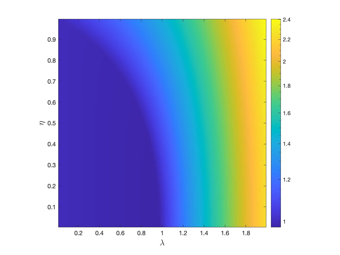
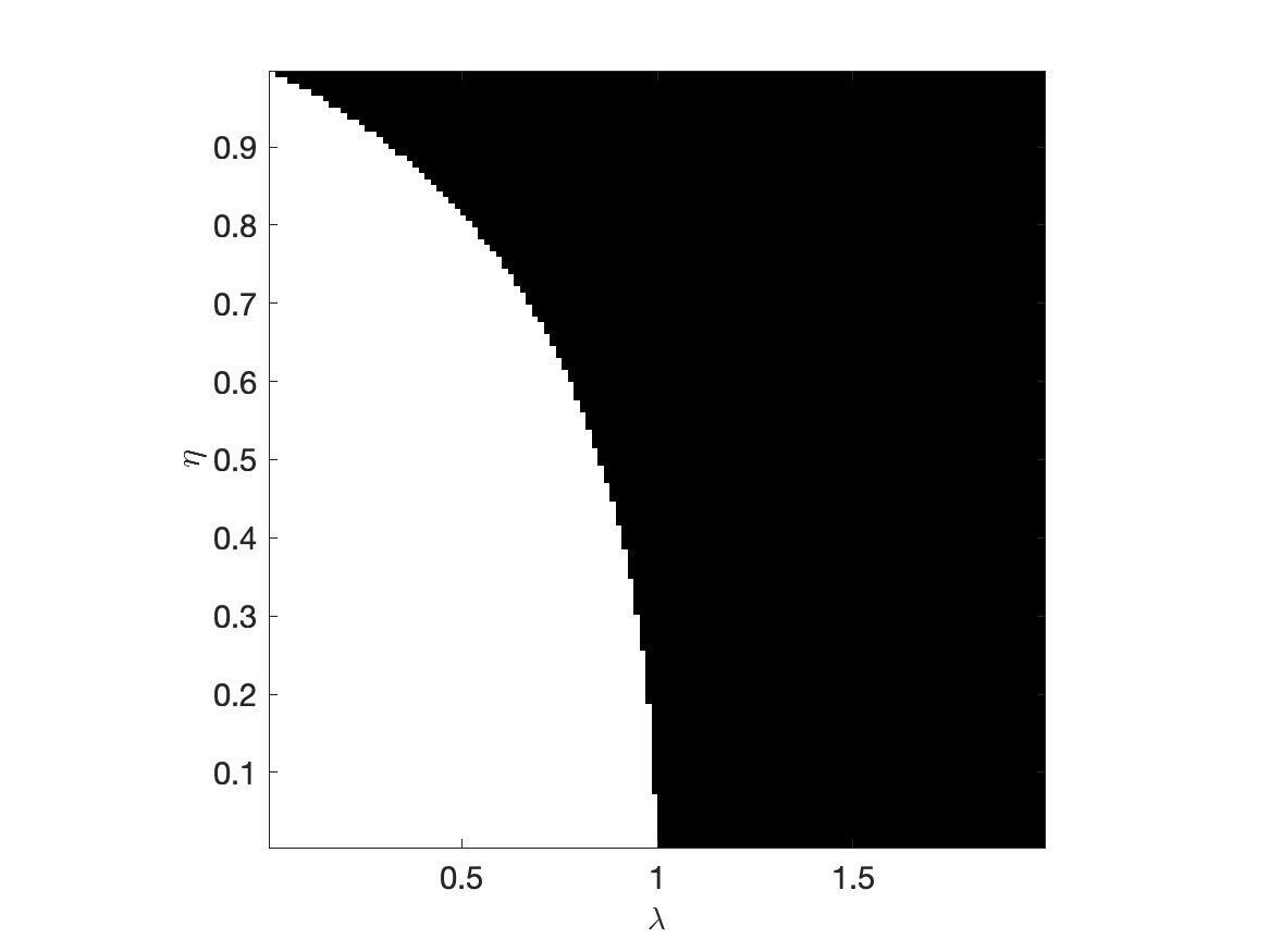
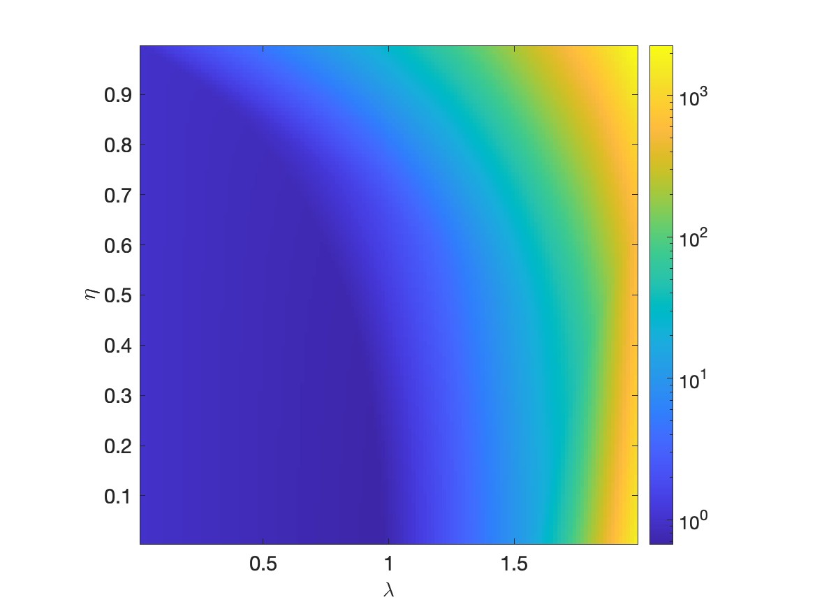
Figure 2: Stationary case: Lipschitz constant of the VNN as a function of $\lambda$ and $\eta$. First row: $\theta_{1}$, second one: $\theta_{15}/2^{14}$. First column: numerical value, second one: white if $\theta_{m}/2^{m-1}\leq 1$.

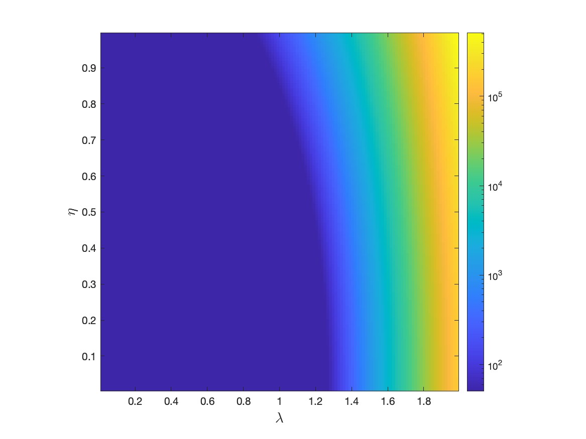
Figure 3: Stationary case: Difference $(\theta_{1})^{15}-\theta_{15}/2^{14}$ for the VNN in the stationary case as a function of $\lambda$ and $\eta$.

Figure 4 illustrates a similar behavior for the Lipschitz constant $\overline{\theta}_{15}/2^{14}$, based on the use of a semi-norm on the VNN output, which has been computed by using Proposition 4.5. The bottom map displays the difference between $\theta_{15}/2^{14}$ and $\overline{\theta}_{15}/2^{14}$, which, as shown in (55), is always nonnegative.

Lastly, for the network with a single input and a single output, Figure 5 presents the Lipschitz constant $\widehat{\theta}_{15}/2^{14}$, computed using Proposition 4.6, for two different operator choices, $F=0$ and $F={\mathchoice{\rm 1\mskip-4.0mul}{\rm 1\mskip-4.0mul}{\rm 1\mskip-4.5mul}{\rm 1\mskip-5.0mul}}$. We observe that selecting $F=0$ results in greater stability compared to $F={\mathchoice{\rm 1\mskip-4.0mul}{\rm 1\mskip-4.0mul}{\rm 1\mskip-4.5mul}{\rm 1\mskip-5.0mul}}$, which aligns with Proposition 4.7.

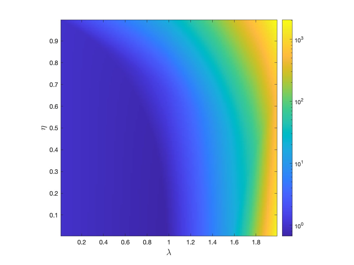
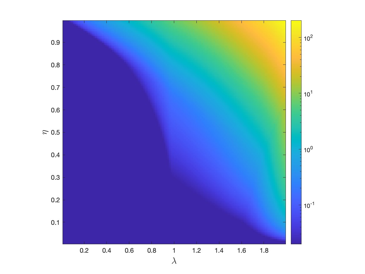
Figure 4: Stationary case: Lipschitz constant of the network with inputs $(x_{0},b_{0})$ and output $x_{15}$ as a function of $\lambda$ and $\eta$. Top left: $\overline{\theta}_{15}/2^{14}$. Top right: white when $\overline{\theta}_{15}/2^{14}<1$. Botton: Difference $\theta_{15}-\overline{\theta}_{15}$.

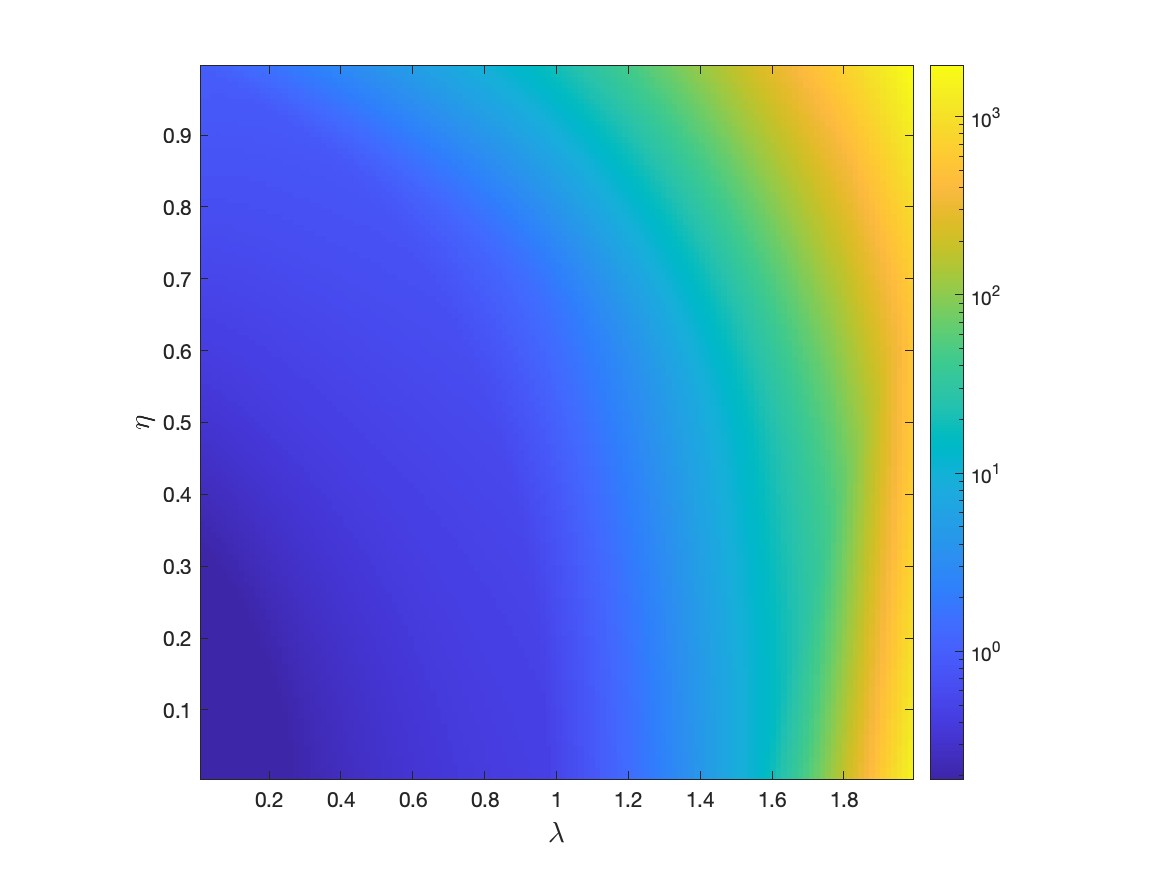
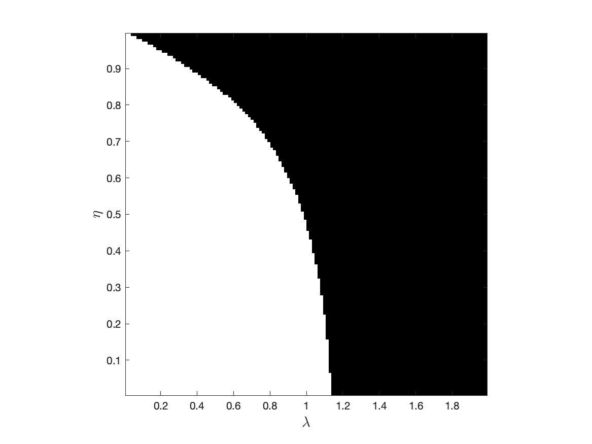
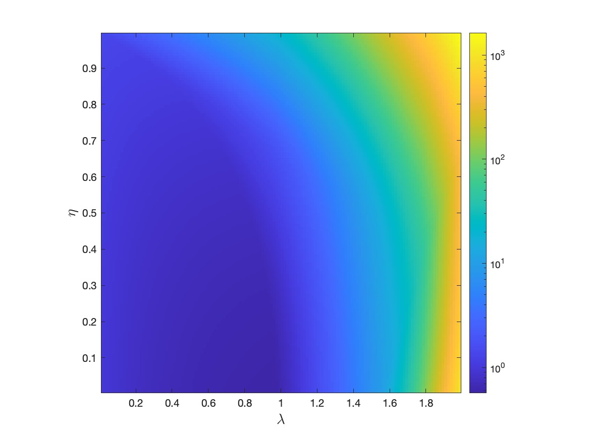
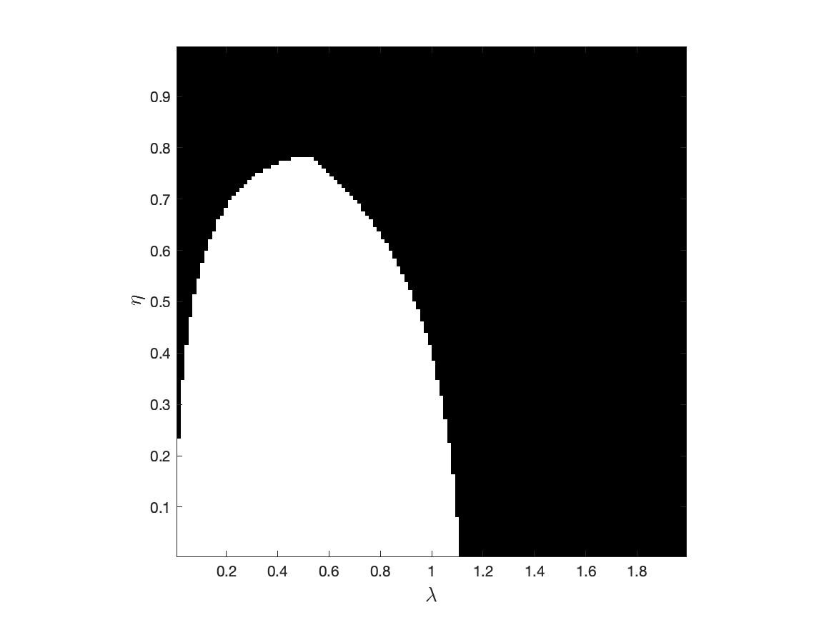
Figure 5: Stationary case: Lipschitz constant $\widehat{\theta}_{15}/2^{14}$ a function of $\lambda$ and $\eta$. First row: $F=0$, second one: $F={\mathchoice{\rm 1\mskip-4.0mul}{\rm 1\mskip-4.0mul}{\rm 1\mskip-4.5mul}{\rm 1\mskip-5.0mul}}$. First column: numerical value, second one: white if $\widehat{\theta}_{15}/2^{14}\leq 1$.

5.2 Nonstationary case

We now consider the scenario most commonly encountered in unrolled algorithms, where the parameter values vary across layers. In our experiments, we set

$$(\forall n\in\{1,\ldots,m\})\quad D_{n}=\sqrt{\tau_{n}}\begin{bmatrix}\nabla_{\rm H}\\ \nabla_{\rm V}\end{bmatrix},$$

and choose $T$ as a two-dimensional $5\times 5$ uniform blur such that $\|T\|=1$. Parameters $\{\tau_{n}\}_{1\leq n\leq m}\subset[0.099,0.0249]$ and $\{\lambda_{n}\}_{1\leq n\leq m}\subset[0.5128,0.9585]$, typical of those learned from an image dataset, are used. The value of $(\eta_{n})_{1\leq n\leq m}$ and $(\chi_{n})_{1\leq n\leq m}$ are set to 0.98 and $10^{-3}$, respectively, although setting the latter strong convexity moduli to zero results in only a slight reduction in the estimated Lipschitz regularity. The weighted norm is defined similarly to the previous example (see (65)).

Figure 6 illustrates the variations in the Lipschitz constant estimates $\theta_{n}/2^{n-1}$, $\overline{\theta}_{n}/2^{n-1}$, and $\widehat{\theta}_{n}/2^{n-1}$ as a function of the layer index $n$. We also compare the proposed estimates with the lower and upper bounds derived in Propositions 4.2, 4.5, and 4.6. It can be observed that the proposed bounds are significantly tighter than the separable lower bounds. While the resulting values exceed 1, they remain within a satisfactory order of magnitude when compared to those encountered in sensitive networks [44].

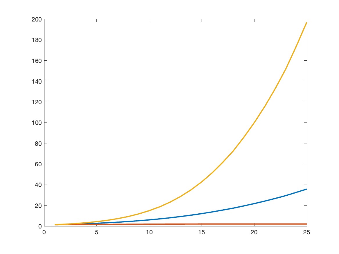
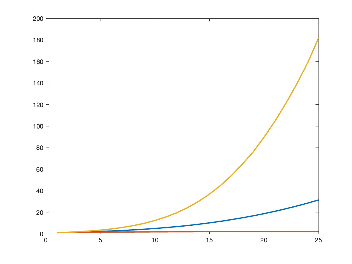
Figure 6: Nonstationary case. From top to bottom: $\theta_{n}/2^{n-1}$, $\overline{\theta}_{n}/2^{n-1}$, and $\widehat{\theta}_{n}/2\textasciidieresis{n-1}$ versus $n$ (in blue), and the corresponding upper bound (in orange) and lower bound (in red). For $\widehat{\theta}_{n}/2^{n-1}$, $F={\mathchoice{\rm 1\mskip-4.0mul}{\rm 1\mskip-4.0mul}{\rm 1\mskip-4.5mul}{\rm 1\mskip-5.0mul}}$.

6 Conclusion

Unrolling optimization algorithms into neural architectures offers significant advantages, including a reduced number of parameters to learn, efficient GPU implementation, and the ability to optimize the quality of the results using relevant loss functions. However, there is currently a lack of theoretical analysis for these structures.
In this work, by leveraging tools from fixed-point theory, we conducted an analysis of the robustness of an unrolled version of the forward-backward algorithm, extending the work in [34], where sensitivity to observed data was overlooked. Our analysis relies on Lipschitz bounds that are computationally efficient (with quadratic complexity) and tighter than the separable bounds commonly used in the neural network community [42].
We acknowledge, however, that these bounds are not optimal. Future work could focus on deriving tighter bounds to further refine the analysis. Additionally, exploring more general proximal algorithms beyond the one considered in this study would be an interesting direction. Finally, we believe the $\alpha$-averaging properties we established could inspire the design of recurrent networks in the spirit of [40].

Acknowledgements

The work by J.-C. Pesquet was supported by the ANR Chair in Artificial Intelligence BRIDGEABLE. E. Chouzenoux acknowledges support from the European Research Council Starting Grant MAJORIS ERC-2019-STG-850925.

Appendix A Stationary case.

In the stationary case, for every $p$, $\beta_{p}^{(n)}=\beta_{p}$. In addition, $\eta_{1,m}=\eta^{m}$, $\beta_{1,m,p}=\beta_{p}^{m}$, and (23) simplifies to

$$\widetilde{\beta}_{1,m,p}=\frac{\lambda}{1+\lambda\chi}\sum_{j=0}^{m-1}\beta_{p}^{j}\eta^{m-j-1}.$$

Then, it follows from (36) that necessary conditions for $\theta_{m}/2^{m-1}=1$ are

$$(\forall p)\quad\begin{cases}|\beta_{p}|\leq 1\\ \displaystyle\varpi_{p}\Big{(}\frac{\lambda}{1+\lambda\chi}\Big{)}^{2}\Big{(}\sum_{j=0}^{m-1}\beta_{p}^{j}\eta^{m-j-1}\Big{)}^{2}+\eta^{2m}\leq 1\quad\Rightarrow\eta<1\;.\end{cases}$$

The first condition is classical for the convergence of the proximal gradient algorithm and it is satisfied if and only if $\lambda\sup_{p}(\beta_{T,p}+\beta_{D,p})\leq 2$.

Furthermore, (36) yields the following sufficient condition for the VNN to be 1-Lipschitz:

$$(\forall p)\quad\beta_{p}^{2}+\varpi_{p}\Big{(}\frac{\lambda}{1+\lambda\chi}\Big{)}^{2}+\eta^{2}\leq 1\;,$$

which, by virtue of (21), is also equivalent to

$$(\forall p)\quad\big{(}1-\lambda(\beta_{T,p}+\beta_{D,p})\big{)}^{2}+\varpi_{p}\lambda^{2}+(1+\lambda\chi)^{2}(\eta^{2}-1)\leq 0\;.$$ (66)

As expected, the strong convexity of the regularizing function $g$ allows this condition to be more easily satisfied since $\eta^{2}-1\leq 0$. Let us focus on the case when $\chi=0$, which provides the following sufficient condition for (66):

$$(\forall p)\quad((\beta_{T,p}+\beta_{D,p})^{2}+\varpi_{p})\lambda^{2}-2(\beta_{T,p}+\beta_{D,p})\lambda+\eta^{2}\leq 0.$$

These inequalities can be satisfied only if

$$(\forall p)\quad\begin{cases}(\beta_{T,p}+\beta_{D,p})^{2}-\eta^{2}((\beta_{T,p}+\beta_{D,p})^{2}+\varpi_{p})\geq 0\\ \lambda_{1,p}(\eta)\leq\lambda\leq\lambda_{2,p}(\eta),\end{cases}$$

where $\lambda_{1,p}(\eta)$ and $\lambda_{2,p}(\eta)$ are the smallest and largest roots of the quadratic polynomial $((\beta_{T,p}+\beta_{D,p})^{2}+\varpi_{p})\lambda^{2}-2(\beta_{T,p}+\beta_{D,p})\lambda+\eta^{2}$. The first inequalities are satisfied if and only if

$$\eta\leq\inf_{p}\frac{\beta_{T,p}+\beta_{D,p}}{\sqrt{(\beta_{T,p}+\beta_{D,p})^{2}+\varpi_{p}}}$$

while the second require that $\sup_{p}\lambda_{1,p}(\eta)\leq\inf_{p}\lambda_{2,p}(\eta)$.

References

- \bibcommenthead
- Bertero et al. [2009] Bertero, M., Boccacci, P., Desiderà, G., Vicidomini, G.: Image deblurring with Poisson data: from cells to galaxies. Inverse Problems 25(12), 123006 (2009)
- Chouzenoux et al. [2012] Chouzenoux, E., Moussaoui, S., Idier, J.: Majorize–minimize linesearch for inversion methods involving barrier function optimization. Inverse Problems 28(6), 065011 (2012)
- Wu et al. [2020] Wu, Z., Sun, Y., Matlock, A., Liu, J., Tian, L., Kamilov, U.S.: SIMBA: Scalable inversion in optical tomography using deep denoising priors. IEEE Journal of Selected Topics in Signal Processing 14(6), 1163–1175 (2020)
- Arsenault et al. [2017] Arsenault, L.-F., Neuberg, R., Hannah, L.A., Millis, A.J.: Projected regression method for solving Fredholm integral equations arising in the analytic continuation problem of quantum physics. Inverse Problems 33(11), 115007 (2017)
- Cherni et al. [2017] Cherni, A., Chouzenoux, E., Delsuc, M.-A.: PALMA, an improved algorithm for DOSY signal processing. The Analyst 142(5), 772–779 (2017)
- Yu et al. [2019] Yu, Y., Si, X., Hu, C., Zhang, J.: A review of recurrent neural networks: LSTM cells and network architectures. Neural computation 31(7), 1235–1270 (2019)
- Tang et al. [2022] Tang, W., Chouzenoux, E., Pesquet, J.-C., Krim, H.: Deep transform and metric learning network: Wedding deep dictionary learning and neural network. Neurocomputing 509, 244–256 (2022)
- Combettes and Wajs [2005] Combettes, P.L., Wajs, V.R.: Signal recovery by proximal forward-backward splitting. Multiscale Modeling & Simulation 4(4), 1168–1200 (2005)
- Combettes and Pesquet [2011] Combettes, P.L., Pesquet, J.-C.: Proximal splitting methods in signal processing. In: al., H.H.B. (ed.) Fixed-point Algorithms for Inverse Problems in Science and Engineering. Springer Optimization and Its Applications, vol. 49, pp. 185–212. Springer, New York, NY (2011)
- Hegland [1995] Hegland, M.: Variable Hilbert scales and their interpolation inequalities with applications to Tikhonov regularization. Applicable Analysis 59(1-4), 207–223 (1995)
- Hofmann and Yamamoto [2005] Hofmann, B., Yamamoto, M.: Convergence rates for Tikhonov regularization based on range inclusions. Inverse Problems 21(3), 805 (2005)
- Åkesson and Daun [2008] Åkesson, E.O., Daun, K.J.: Parameter selection methods for axisymmetric flame tomography through Tikhonov regularization. Applied optics 47(3), 407–416 (2008)
- Daun et al. [2006] Daun, K.J., Thomson, K.A., Liu, F., Smallwood, G.J.: Deconvolution of axisymmetric flame properties using Tikhonov regularization. Applied optics 45(19), 4638–4646 (2006)
- Engl [1996] Engl, H.W.: Regularization of Inverse Problems. Kluwer Academic Publishers, Dordrecht Boston (1996)
- Hansen [1999] Hansen, P.C.: The l-curve and its use in the numerical treatment of inverse problems (1999)
- Antholzer et al. [2019] Antholzer, S., Haltmeier, M., Schwab, J.: Deep learning for photoacoustic tomography from sparse data. Inverse Problems in Science and Engineering 27(7), 987–1005 (2019)
- Kofler et al. [2018] Kofler, A., Haltmeier, M., Kolbitsch, C., Kachelrieß, M., Dewey, M.: A u-nets cascade for sparse view computed tomography. In: International Workshop on Machine Learning for Medical Image Reconstruction, pp. 91–99 (2018). Springer
- Hammernik et al. [2018] Hammernik, K., Klatzer, T., Kobler, E., Recht, M.P., Sodickson, D.K., Pock, T., Knoll, F.: Learning a variational network for reconstruction of accelerated MRI data. Magnetic Resonance in Medicine 79(6), 3055–3071 (2018)
- Adler and Öktem [2017] Adler, J., Öktem, O.: Solving ill-posed inverse problems using iterative deep neural networks. Inverse Problems 33(12), 124007 (2017)
- Aggarwal et al. [2018] Aggarwal, H.K., Mani, M.P., Jacob, M.: MoDL: Model-based deep learning architecture for inverse problems. IEEE Transactions on Medical Imaging 38(2), 394–405 (2018)
- Meinhardt et al. [2017] Meinhardt, T., Moller, M., Hazirbas, C., Cremers, D.: Learning proximal operators: Using denoising networks for regularizing inverse imaging problems. In: Proceedings of the IEEE International Conference on Computer Vision (ICCV 2017), Venice, Italy, pp. 1781–1790 (2017)
- Pesquet et al. [2021] Pesquet, J.-C., Repetti, A., Terris, M., Wiaux, Y.: Learning maximally monotone operators for image recovery. SIAM Journal on Imaging Sciences 14(3) (2021)
- Hasannasab et al. [2020] Hasannasab, M., Hertrich, J., Neumayer, S., Plonka, G., Setzer, S., Steidl, G.: Parseval proximal neural networks. Journal of Fourier Analysis and Applications 26(4) (2020)
- Galinier et al. [2020] Galinier, M., Prato, M., Chouzenoux, E., Pesquet, J.-C.: A hybrid interior point - deep learning approach for Poisson image deblurring. In: Proceedings of the IEEE 30th International Workshop on Machine Learning for Signal Processing (MLSP 2020), Espoo, Finland, pp. 1–6 (2020)
- Li et al. [2020] Li, H., Schwab, J., Antholzer, S., Haltmeier, M.: NETT: Solving inverse problems with deep neural networks. Inverse Problems 36(6), 065005 (2020)
- Bubba et al. [2021] Bubba, T.A., Galinier, M., Lassas, M., Prato, M., Ratti, L., Siltanen, S.: Deep neural networks for inverse problems with pseudodifferential operators: an application to limited-angle tomography. SIAM Journal on Imaging Sciences 14(2) (2021)
- Gilton et al. [2019] Gilton, D., Ongie, G., Willett, R.: Neumann networks for linear inverse problems in imaging. IEEE Transactions on Computational Imaging 6, 328–343 (2019)
- Ryu et al. [2019] Ryu, E., Liu, J., Wang, S., Chen, X., Wang, Z., Yin, W.: Plug-and-play methods provably converge with properly trained denoisers. In: Proceedings of the International Conference on Machine Learning (ICML 2019), Long Beach, CA, pp. 5546–5557 (2019)
- Sun et al. [2019] Sun, Y., Wohlberg, B., Kamilov, U.S.: An online plug-and-play algorithm for regularized image reconstruction. IEEE Transactions on Computational Imaging 5(3), 395–408 (2019)
- Hurault et al. [2022] Hurault, S., Leclaire, A., Papadakis, N.: Proximal denoiser for convergent plug-and-play optimization with nonconvex regularization. In: Proceedings of the International Conference on Machine Learning (ICML 2022), vol. 16. Baltimore, MD, pp. 9483–9505 (2022)
- Gregor and LeCun [2010] Gregor, K., LeCun, Y.: Fast approximations of sparse coding. In: Proceedings of the International Conference on Machine Learning (ICML 2010), Haifa, Israel, pp. 399–406 (2010)
- Borgerding and Schniter [2016] Borgerding, M., Schniter, P.: Onsager-corrected deep learning for sparse linear inverse problems. In: Proceedings of the IEEE Global Conference on Signal and Information Processing (GlobalSIP 2016), Greater Washington, DC, pp. 227–231 (2016)
- Jin et al. [2017] Jin, K.H., McCann, M.T., Froustey, E., Unser, M.: Deep convolutional neural network for inverse problems in imaging. IEEE Transactions on Image Processing 26(9), 4509–4522 (2017)
- Bertocchi et al. [2020] Bertocchi, C., Chouzenoux, E., Corbineau, M.-C., Pesquet, J.-C., Prato, M.: Deep unfolding of a proximal interior point method for image restoration. Inverse Problems 36(3), 034005 (2020)
- Natarajan and Caro [2020] Natarajan, S.K., Caro, M.A.: Particle swarm based hyper-parameter optimization for machine learned interatomic potentials. arXiv preprint arXiv:2101.00049 (2020)
- Monga et al. [2021] Monga, V., Li, Y., Eldar, Y.C.: Algorithm unrolling: Interpretable, efficient deep learning for signal and image processing. IEEE Signal Processing Magazine 38(2), 18–44 (2021)
- Gharbi et al. [2024] Gharbi, M., Chouzenoux, E., Pesquet, J.-C.: An unrolled half-quadratic approach for sparse signal recovery in spectroscopy. Signal Processing 218, 109369 (2024)
- Le et al. [2024] Le, H.T.V., Repetti, A., Pustelnik, N.: Unfolded proximal neural networks for robust image gaussian denoising. IEEE Transactions on Image Processing 33, 4475–4487 (2024)
- Genzel et al. [2020] Genzel, M., Macdonald, J., März, M.: Solving inverse problems with deep neural networks–robustness included? arXiv preprint arXiv:2011.04268 (2020)
- Combettes and Pesquet [2020a] Combettes, P.L., Pesquet, J.-C.: Deep neural network structures solving variational inequalities. Set-Valued and Variational Analysis, 1–28 (2020)
- Combettes and Pesquet [2020b] Combettes, P.L., Pesquet, J.-C.: Lipschitz certificates for layered network structures driven by averaged activation operators. SIAM Journal on Mathematics of Data Science 2(2), 529–557 (2020)
- Serrurier et al. [2021] Serrurier, M., Mamalet, F., González-Sanz, A., Boissin, T., Loubes, J.-M., Barrio, E.: Achieving robustness in classification using optimal transport with hinge regularization. In: Proceedings of the IEEE/CVF Conference on Computer Vision and Pattern Recognition (CVPR 2021), virtual (2021)
- Cisse et al. [2017] Cisse, M., Bojanowski, P., Grave, E., Dauphin, Y., Usunier, N.: Parseval networks: Improving robustness to adversarial examples. In: Proceedings of the International Conference on Machine Learning (ICML 2017), Sydney, Australia, pp. 854–863 (2017)
- Neacşu et al. [2024a] Neacşu, A., Pesquet, J.-C., Burileanu, C.: EMG-based automatic gesture recognition using Lipschitz-regularized neural networks. ACM Transactions on Intelligent Systems and Technology 18, 1–25 (2024)
- Neacşu et al. [2024b] Neacşu, A., Pesquet, J.-C., Vasilescu, V., Burileanu, C.: ABBA neural networks: Coping with positivity, expressivity, and robustness. SIAM Journal on Mathematics of Data Science 6, 649–678 (2024)
- Bauschke and Combettes [2011] Bauschke, H.H., Combettes, P.L.: Convex Analysis and Monotone Operator Theory in Hilbert Spaces vol. 408. Springer, New York (2011)
- Terris et al. [2019] Terris, M., Abdulaziz, A., Dabbech, A., Jiang, M., Repetti, A., Pesquet, J.-C., Wiaux, Y.: Deep post processing for sparse image deconvolution. In: Signal Processing with Adaptive Sparse Structured Representations (SPARS), Toulouse, France, p. 2 (2019)