Remark on the Emergence of Color Superconductivity for Gauge Theories
in General Spacetime Dimensions from simple Holographic Models

Abstract

We generalize the concept of holography for the color superconductivity (CSC) phase by considering $d$-dimensional Anti de Sitter (AdS) space instead of the traditional 6 dimensions. The corresponding dual field theory is an arbitrary confining gauge theory with $SU(N_{c})$ symmetry, like quantum chromodynamics (QCD) CSC. We then use a holographic model based on Einstein-Maxwell gravity in $d$-dimensional AdS spacetime to study this phenomenon in both confinement and deconfinement phase, study the confinement$-$deconfinement phase transition and the condition for the $N_{c}=2$ CSC phase with $d=4$ case, one special case from Vu2024 .

I Introduction

In quantum chromodynamics (QCD) theory, color superconductivity (CSC) phase is one of interesting topics. It is the pairing of two quarks in one Cooper pair condensate, the diquark. We believe that this phase exists in the inner cores of heavy neutron stars fadafan2018 ; Fadafan2021 because the CSC phase appears at high chemical potential and low temperature and we can probe this phase from observe the gravitational wave by LIGO LIGO2017 on a neutron star collision.

One way to study the CSC phase that we use the holographic principle or the AdS/CFT correspondence Maldacena1997 ; Witten98 ; Gubser1998 to approach. In this framework a weakly coupled gravity theory in $d$-dimensional anti-de Sitter (AdS) spacetime correspond to a strongly coupled conformal field theory (CFT) on the $(d-1)$-dimensional boundary of that spacetime. Within this frame work we can study one problem in the CFT with strong coupling constant by the translate this to gravity problem at weak coupling constant via holographic dictionary. In QCD, the CSC phase appear in high chemical potential and low temperature (below the QCD scale). To describe this by holographic QCD, we introduce an additional compact extra dimension on the boundary that corresponds to the QCD scale. This technique of geometrizing a physical effect has also been employed in classical physics phan2021curious . As a result, for the AdS theory to be dual to our four dimensional spacetime universe, the boundary becomes $R^{3,1}\times S^{1}$, and its bulk spacetime having six dimensions Basu.et.al.2011 . This differ with the traditional holographic QCD Vu2020 where we studied by the five dimension bulk and the four dimensions found in holographic models of metallic superconductivity Horowitz2008 ; Hartnoll2008 .

In the first study of the holographic model for CSC phase Basu.et.al.2011 , the authors considered the Einstein-Maxwell gravity and the standard Maxwell interaction (i.e. $\mathcal{L}_{\text{Maxwell}}=-\frac{1}{4}F^{2}$) in six-dimensional AdS spacetime. It is important to note that $\mathcal{L}_{\text{Maxwell}}$ differs from the Maxwell power-law holographic model studied in Cao Nam2022 . There, an AdS soliton with scalar hair corresponds to the confinement phase, while a Reissner$-$Nordström (RN) AdS black hole with scalar hair is dual to the deconfinement phase. The scalar hair correspond to the diquarks operator in the boundary, called $s-$waves color superconductivity, which only appear when the chemical potential $\mu$ exceeds a critical value $\mu_{c}$ and, in the deconfinement phase, the temperature $T$ is below a critical temperature, $T_{c}$ which depend on $\mu_{c}$ Basu.et.al.2011 . It was believed that color superconductivity could not occur in the confinement phase and only appeared in the deconfinement phase, until Kazuo et al. Kazuo2019 has demonstrated that, under Einstein-Maxwell gravity, the CSC phase is possible, but limited to cases with a single color $N_{c}=1$. In more detail, the Breitenlohner-Freedman (BF) bound BF1 ; BF2 for the stability of the scalar field (representing diquark Cooper pair) is broken when $N_{c}<1.89$, thus we cannot study the CSC phase with $N_{c}=2$. This problem can be solved by modifying the gravity framework or the Maxwell interaction law, as suggested in Cao Nam2021 and Cao Nam2022 .

Here, there is one open question that is what happen if we generalize the conception of CSC phase for an arbitrary $SU(N_{c})$ and build one holographic model for this phase with an arbitrary $d$ dimension. In the previous project, Vu2024 we explored the holographic model for the CSC phase in general case but without the confinement phase. In this project, we add the confinement phase (confined gauge theory) dual with the AdS soliton solution. We consider the confinement$-$deconfinement phase transition in the $d-$dimension and consider the CSC phase in the confinement and deconfinement phases. In Section II, we introduce the $d$-dimensional gravitational dual model of interest for the CSC phase transition. In Section III, we analyze the CSC phase, deriving the conditions on $(d,N_{c})$ for the formation of Cooper pairs on both confinement and the deconfinement phases, we also discuss the $4d$ confinement$-$deconfinement phase transition. Finally, in Section IV, we conclude with the main results and mention some open questions and interesting future directions.

II Holographic Model setup

First of all, we redefine the conception of the generalized color superconductivity phase. In this paper, it is one arbitrary Cooper pair condensate (we called the Cooper pair not diquark because we don’t consider QCD CSC) for one arbitrary $SU(N_{c})$ confined gauge theory instead of the QCD color superconductivity only for the $SU(3)_{C}$ gauge theory. In this paper, we will consider the CSC phase in general confined gauge theory, like the QCD CSC case. From this assumption we have the confinement-deconfinement phase transition and we find the CSC phase in both the confinement and deconfinement phases. And, like the holographic QCD CSC we also have one compact dimension $y$, which corresponds to the scale analogy of the QCD scale. Hence, the boundary becomes $R^{d-2}\times S^{1}$ and the bulk $R^{d-1}\times S^{1}$ instead of $R^{d-1}$ and $R^{d}$ inVu2024 . The action for the $d$-dimensional Einstein-Maxwell gravity during the CSC phase transition is given by Emparan2014 :

$$\begin{split}S=&\int d^{d}x\sqrt{-g}\Bigg{[}\mathcal{R}+\frac{(d-1)(d-2)}{L^{2}}\\ &-\frac{1}{4}F^{2}-|(\partial_{\mu}-iqA_{\mu})\psi|^{2}-m^{2}|\psi|^{2}\Bigg{]}\ ,\end{split}$$ (1)

where $F_{\mu\nu}=\partial_{\mu}A_{\nu}-\partial_{\nu}A_{\mu}$ and the cosmological constant is determined by $\Lambda=-\frac{(d-1)(d-2)}{2L^{2}}$. We then set the AdS radius $L=1$ for convenience. Here, the $U(1)$ gauge field $A_{\mu}$ dual to the current that analogous to the baryon number current in the CSC phase of QCD or the electric current in metallic superconductivity. The complex scalar field $\psi$ is dual to the boundary Cooper pair scalar field operator; specifically, in the holographic model for the QCD color superconductivity, it corresponds to the diquark Cooper pair scalar field operator (the $s-$wave CSC phase). The charge $q$ of this scalar field $\psi$ is associated with quantity in general, called general CSC charges, like the baryon number of the diquark in QCD color superconductivity, and its value is given by

$$q=\frac{2}{N_{c}}\ ,$$ (2)

in which $N_{c}$ counts number of colors.

To further simplify our model from Eq. (1), we focus on $s-$wave CSC (may be the $p-$wave or $d-$wave CSC phase exist but we don’t study these in this project), in which the vector field $A_{\mu}$ and complex scalar field $\psi$ follow the ansatz:

$$A_{\mu}dx^{\mu}=\phi(r)dt\ ,\ \psi=\psi(r)\ ,$$ (3)

where the variations are purely radial. The $s-$wave CSC phase appears from the condensation of the scalar field Cooper pairs, ($p-$wave and $d-$wave the Cooper pars is the vector fields) corresponding to the spontaneous broken of the $U(1)$ gauge symmetry. Assuming that the charge is fixed, the condensation of the scalar field $\psi$ is controlled by the chemical potential, analogous to the baryon chemical potential of quarks in the QCD color superconductivity. At the critical chemical potential the scalar Cooper pair condensation is created, we have the dual bulk scalar field $\psi(r)=0$. Near the critical chemical potential, the value of the bulk scalar field $\psi\approx 0$ and we can neglect the back reaction of the bulk scalar field on the spacetime. Therefore, the back reaction of the matter field is only contributed by the $U(1)$ gauge field $A_{\mu}$.

In this model, we includes the confinement phase; thus, we will find the CSC phase in both confinement phase and deconfinement phase. In the deconfinement phase which dual to black hole on the bulk, the phase transition of the CSC phase occurs at a critical temperature $T_{c}$ Basu.et.al.2011 , this temperature is associated with the critical chemical potential $\mu_{c}$ (similar to the QCD CSC phase in the deconfinement phase). And the scalar bulk field which correspond to the Cooper pair appears when the chemical potential $\mu>\mu_{c}$ or the temperature $T<T_{c}$, called the scalar hair of black hole. In the holographic dictionary, because there is one scalar hair, the spacetime geometry dual to this phase is described by the Reissner-Nordström (RN) planar black hole solution, with the metric given by the following ansatz:

$$ds^{2}=r^{2}\Big{[}-f(r)dt^{2}+h_{ij}dx^{i}dx^{j}+dy^{2}\Big{]}+\frac{dr^{2}}{r^{2}f(r)}\ ,$$ (4)

where $h_{ij}dx^{i}dx^{j}=dx_{1}^{2}+...+dx_{d-3}^{2}$ is the line element of the $(d-3)$-dimension hypersurface and the direction $y$ is compacted with the radius $R_{y}$. The event horizon radius $r_{+}$ satisfies

$$f(r_{+})=0\ .$$ (5)

In the holographic dictionary, the temperature of the boundary field theory is associated with the Hawking temperature of this $d$-dimensional RN planar AdS black hole, i.e.

$$T=T_{H}\equiv\frac{r_{+}^{2}f^{\prime}(r_{+})}{4\pi}\ .$$ (6)

Using the ansatz Eq.(3), we can obtain the classical equations of motion for the temporal component of the vector field $\phi$ and the complex scalar field $\psi$ to be:

$$\begin{split}&\phi^{\prime\prime}(r)+\frac{d-2}{r}\phi^{\prime}(r)-\frac{2q^{2}\psi^{2}(r)}{r^{2}f(r)}\phi(r)=0\ ,\\ &\psi^{\prime\prime}(r)+\left[\frac{f^{\prime}(r)}{f(r)}+\frac{d}{r}\right]\psi^{\prime}(r)\\ &+\frac{1}{r^{2}f(r)}\left[\frac{q^{2}\phi^{2}(r)}{r^{2}f(r)}-m^{2}\right]\psi(r)=0\ ,\end{split}$$ (7)

in which the blackening function $f(r)$ is given by Nam2021 ,Nam2019 :

$$f(r)=1-\left(1+\frac{3\mu^{2}}{8r_{+}^{2}}\right)\left(\frac{r_{+}}{r}\right)^{d-1}+\frac{3\mu^{2}r_{+}^{d}}{8r^{d+2}}$$ (8)

To check the blackening function, in the case of the $d=6$-dimensional spacetime, this expression becomes:

$$f(r)=1-\left(1+\frac{3\mu^{2}}{8r^{2}_{+}}\right)\left(\frac{r_{+}}{r}\right)^{5}+\frac{3\mu^{2}r_{+}^{6}}{8r^{8}}\ ,$$

which is equivalent to the holographic model for the QCD CSC in the deconfinement region Kazuo2019 .

In deconfinement phase, the temperature $T$ of the color superconductivity phase live on the boundary correspond to the Hawking temperature $T_{H}$ observed in the bulk, as mentioned in Eq. (6). Hence:

$$T=\frac{r_{+}^{2}f^{\prime}(r_{+})}{4\pi}=\frac{1}{4\pi}\left[(d-1)r_{+}-\frac{9\mu^{2}}{8r_{+}}\right]\ .$$ (9)

From the physical condition that these thermal temperatures cannot be negative, we have the constraint for the chemical potential $\mu$:

$$\frac{\mu^{2}}{r_{+}^{2}}\leq\frac{8(d-1)}{9}\ .$$ (10)

Near the boundary $(r\rightarrow\infty)$, from the equations of motion Eq. (7), we have the asymptotic forms for the matter fields:

$$\begin{split}\phi(r)&=\mu-\frac{\rho}{r^{d-3}}\ ,\\ \psi(r)&=\frac{J_{C}}{r^{\Delta_{-}}}+\frac{C}{r^{\Delta_{+}}}\ ,\end{split}$$ (11)

where $\mu,\rho,J_{C}$, and $C$ are regarded as the chemical potential, charge density, source, and the condensates vacuum expected value (VEV) of the Cooper pair operator dual to $\psi$ (like the diquark Cooper pair in QCD), respectively. In this case, the conformal dimensions $\Delta_{\pm}$ read:

$$\Delta_{\pm}=\frac{1}{2}\left[(d-1)\pm\sqrt{(d-1)^{2}+4m^{2}}\right]\ ,$$ (12)

and the BF bound – as follows from BF1 ; BF2 – is:

$$m^{2}\geq-\frac{(d-1)^{2}}{4}\ .$$ (13)

This is the stability condition for the field $\psi$. To simplify, we set $\Delta_{-}=1$ Nam2019 , which leads to:

$$m^{2}=2-d\ ,$$ (14)

and therefore obtain $\Delta_{+}=d-2$. Note that in this setting, two components of $\psi$ are normalizable modes and $m^{2}$ always satisfies Eq. (13). Thus, Eq. (11) becomes:

$$\psi(r)=\frac{J_{C}}{r}+\frac{C}{r^{d-2}}\ .$$ (15)

From Vu2024 we have the boundary condition at

$$\begin{split}&\phi(r_{+})=0\ ,\\ &\psi(r_{+})=r_{+}^{2}\frac{f^{\prime}(r_{+})\psi^{\prime}(r_{+})}{m^{2}}\ .\end{split}$$ (16)

Now we consider the confinement phase. In the confinement phase the temperature $T=0$, the spacetime geometry dual to the confinement phase the AdS soliton solution Natsuume2015 in $d-$dimension and we have

$$ds^{2}=r^{2}(\gamma_{\mu\nu}dx^{\mu}dx^{\nu}+dx_{d-3}^{2}+f(r)dy^{2})+\frac{dr^{2}}{r^{2}f(r)},$$ (17)

with

$$f(r)=1-\left(\frac{r_{0}}{r}\right)^{d-1}$$ (18)

$r_{0}=\frac{2}{(d-1)R_{y}}$ is the radius which analogy with the event horizon. From this ansatz we obtain the equation of motion for the confinement phase

$$\begin{split}&\phi^{\prime\prime}(r)+\left[\frac{d-2}{r}+\frac{f^{\prime}(r)}{f(r)}\right]\phi^{\prime}(r)-\frac{2q^{2}\psi^{2}(r)}{r^{2}f(r)}\phi(r)=0\\ &\psi^{\prime\prime}(r)+\left[\frac{d}{r}+\frac{f^{\prime}(r)}{f(r)}\right]\psi^{\prime}(r)+\frac{1}{r^{2}f(r)}\left[\frac{q^{2}\phi^{2}(r)}{r^{2}}-m^{2}\right]\psi(r)=0\end{split}$$ (19)

The boundary condition at $r_{0}$ Kazuo2019 , Nam2021

$$\begin{split}\phi^{\prime}(r_{0})&=\frac{2q^{2}\psi^{2}(r_{0})}{r_{0}^{2}f^{\prime}(r_{0})}\phi(r_{0})\\ \psi^{\prime}(r_{0})&=-\frac{1}{r_{0}^{2}f^{\prime}(r_{0})}\left(\frac{q^{2}\phi^{2}(r_{0})}{r_{0}^{2}}-m^{2}\right)\psi(r_{0}).\end{split}$$ (20)

And replace the value of $f(r)$ in confinement phase, we get

$$\begin{split}\phi^{\prime}(r_{0})&=\frac{2q^{2}\psi^{2}(r_{0})}{(d-1)r_{0}}\phi(r_{0})\\ \psi^{\prime}(r_{0})&=-\frac{1}{(d-1)r_{0}}\left(\frac{q^{2}\phi^{2}(r_{0})}{r_{0}^{2}}-m^{2}\right)\psi(r_{0})\end{split}$$ (21)

III The emergence of CSC phase with multiple colors

When the chemical potential $\mu$ exceeds the critical value $\mu_{c}$, Cooper pair condensation occurs. Near the critical chemical potential (when $\mu>\mu_{c}$ but still close to $\mu_{c}$), $\psi$ should be approximately $0$, so its back reaction can be neglected. Therefore, the bulk configuration is approximately determined by:

$$S=\int d^{d}x\sqrt{-g}\left(\mathcal{R}-2\Lambda-\frac{1}{4}F^{2}\right)\ .$$ (22)

The solution of the gauge field in this case is simply:

$$\phi(r)=\mu\left[1-\left(\frac{r_{+}}{r}\right)^{d-3}\right]\ ,$$ (23)

in the deconfinement phase duality with the planar RN black hole and

$$\phi(r)=\mu,$$ (24)

in the confinement phase duality to AdS soliton solution, which is consistent with Eq. (11) and Eq. (16).

To probe the confinement-deconfinement phase transition, we need to compute the Euclidean action of the bulk. The general Euclidean action is given by

$$S^{E}=-\int d^{d}x\sqrt{-g}\mathcal{L}$$ (25)

Using Olea2011 for $d>4$ we obtain

$$\begin{split}S^{E}_{2k}&=\beta Vol(\Gamma_{d-2})[(r^{2}f)^{\prime}r^{d-2}|^{\infty}_{r_{+}}\\ &-(r^{2}f)^{\prime}(r^{2}f)^{k-1}|^{\infty}-r^{d-2}\phi\phi^{\prime}|^{\infty}_{r_{+}}]\end{split}$$ (26)

with $d$ is even, $d=2k$ and with $d$ odd we have

$$\begin{split}&S^{E}_{2k+1}=\beta Vol(\Gamma_{2k-1})r^{2k-1}(r^{2}f)^{\prime}|^{\infty}_{r_{+}}\\ &+\beta Vol(\Gamma_{2k-1})kc_{2k}(2k-1)!\\ &\times[r^{2k-1}(r^{2}f)^{\prime}\int_{0}^{1}dt(\frac{-f^{2}}{r^{2}}+t^{2})^{k-1}\\ &+2\int^{1}_{0}dtt(f^{2}-\frac{r(f^{2})^{\prime}}{2})(t^{2}(r^{2}-f^{2}))^{k-1}]|^{\infty}\\ &-\beta Vol(\Gamma_{d-2})r^{d-2}\phi\phi^{\prime}|^{\infty}_{r_{+}}\end{split}$$ (27)

with $t$ is one parameter to express the boundary term becomes the polynomial, Olea2011 and

$$c_{2k}=-\frac{2(-1)^{k-1}}{k(2k-1)!\beta(k,\frac{1}{2})}.$$ (28)

From (26) and (27) we obtain the free energy for the AdS black hole and for AdS soliton when $d$ even.

$$\begin{split}\Omega_{BH{2k}}&=Vol(\Gamma_{d-2})[(r^{2}f)^{\prime}r^{d-2}|^{\infty}_{r_{+}}\\ &-(r^{2}f)^{\prime}(r^{2}f)^{k-1}|^{\infty}-r^{d-2}\phi\phi^{\prime}|^{\infty}_{r_{+}}]\\ &=[-r_{+}^{d-1}-\frac{5d-27}{8}\mu^{2}r_{+}^{d-3}]Vol(\Gamma_{d-2}),\end{split}$$ (29)

with the AdS black hole and with the AdS soliton we have

$$\Omega_{soliton{2k}}=-r_{0}^{d-1}Vol(\Gamma_{d-2}),$$ (30)

for $d=2k$.

When $d$ odd $d=2k+1$ we have the free energy

$$\begin{split}&\Omega_{{2k+1}}=Vol(\Gamma_{2k-1})r^{2k-1}(r^{2}f)^{\prime}|^{\infty}_{r_{+}}\\ &+Vol(\Gamma_{2k-1})kc_{2k}(2k-1)!\\ &\times[r^{2k-1}(r^{2}f)^{\prime}\int_{0}^{1}dt(\frac{-f^{2}}{r^{2}}+t^{2})^{k-1}\\ &+2\int^{1}_{0}dtt(f^{2}-\frac{r(f^{2})^{\prime}}{2})(t^{2}(r^{2}-f^{2}))^{k-1}]|^{\infty}\\ &-Vol(\Gamma_{d-2})r^{d-2}\phi\phi^{\prime}|^{\infty}_{r_{+}}.\end{split}$$ (31)

These formulas can’t apply for $d=4$ case. In $d=4$ case, the Euclidean action becomes

$$S^{E}=S_{grav}+S^{E}_{matter}+S^{E}_{CT}$$ (32)

The gravity action $S_{grav}$ is given by

$$S_{grav}=S_{bulkgrav}+S_{G.H.Y}$$ (33)

We have

$$\begin{split}S_{bulkgrav}&=-\int dX^{4}\sqrt{-g}(R-2\Lambda)=2XR_{y}\beta(4-1)\frac{1}{3}r^{3}\\ &=2XR_{y}\beta r^{3}|^{\infty}_{r_{+}}\end{split}$$ (34)

The Gibbons-Hawking-York term

$$S_{GHY}=-2\int dx^{3}\sqrt{-h}K$$ (35)

Where $K$ is the extrinsic curvature and $h=deth_{ab}$ with $h_{ab}$ the metric in $d-1$ dimension, without $r$. Hence $h_{ab}=(-r^{2}f(r),r^{2},r^{2})$ and $h^{ab}=(\frac{1}{r^{2}f(r)},\frac{1}{r^{2}},\frac{1}{r^{2}})$, and the normal vector is defined by

$$n^{\mu}=\frac{1}{\sqrt{g_{rr}}}\left(\frac{\partial}{\partial r}\right)^{\mu}=\frac{\delta_{r}^{\mu}}{\sqrt{g_{rr}}}$$ (36)

The non zero component of the normal vector is

$$n^{r}=r\sqrt{f(r)}$$ (37)

We have

$$K=\frac{1}{2}h^{ab}n^{r}\partial_{r}h_{ab}=\frac{1}{2}\left(\frac{rf^{\prime}(r)}{\sqrt{f(r)}}+2\sqrt{f(r)}+4\sqrt{f(r)}\right)$$ (38)

and

$$\sqrt{-h}=\sqrt{-(-r^{2}f(r).r^{2}.r^{2})}=r^{3}\sqrt{f(r)}$$ (39)

Hence the G.H.Y term

$$S_{GHY}=\beta R_{y}X(-6r^{3}f(r)-r^{4}f^{\prime}(r))|^{\infty}$$ (40)

The matter part $S^{E}_{matter}$ is given by

$$S^{E}_{matter}=S^{E}_{bulkmatter}+S_{bnd,F}$$ (41)

We have

$$\begin{split}S^{E}_{bulkmatter}&=-XR_{y}\beta\int dr\sqrt{-g}\left(-\frac{1}{4}F^{2}\right)\\ &=-XR_{y}\beta\int dr\sqrt{-g}\left(-\frac{1}{2}g^{00}g^{rr}\phi^{\prime 2}\right)\\ &=-XR_{y}\beta\frac{1}{2}r^{2}\phi(r)\phi^{\prime}(r)|^{\infty}_{r_{+}}\\ &=-XR_{y}\beta\frac{1}{2}\mu^{2}r_{+}\end{split}$$ (42)

and

$$\begin{split}S_{bnd,F}&=XR_{y}\beta\frac{1}{2}\sqrt{-h}n_{a}F^{ab}A_{b}\\ &=XR_{y}\beta\frac{1}{2}\sqrt{-h}n_{r}F^{r0}A_{0}\\ &=-XR_{y}\beta\frac{1}{2}r^{3}\sqrt{f(r)}\frac{1}{r\sqrt{f(r)}}\phi^{\prime}(r)\phi(r)|^{\infty}\\ &=-XR_{y}\beta\frac{1}{2}r^{2}\phi\phi^{\prime}|^{\infty}\\ &=-XR_{y}\beta\frac{1}{2}\mu^{2}r_{+}\end{split}$$ (43)

We have

$$S^{E}{matter}=-XR_{y}\beta\mu^{2}r_{+}$$ (44)

And finally the counter-term action is given by

$$\begin{split}S^{E}_{CT}&=2(d-2)\sqrt{-h}\beta XR_{y}\\ &=4\beta XR_{y}r^{3}\sqrt{f(r)}\end{split}$$ (45)

From (45), (34), (40), (44), we obtain the Euclidean action for $d=4$ case

$$S^{E}_{4dbh}=-r^{3}_{+}\left(1+\frac{5\mu^{2}}{8r_{+}^{2}}\right)\beta XR_{y},$$ (46)

and with the 4d AdS soliton case

$$S^{E}_{4dsoliton}=-r_{0}^{3}\beta XR_{y}$$ (47)

Hence, at $4d$ we have $\Omega_{4dbh}=-r^{3}_{+}\left(1+\frac{5\mu^{2}}{8r_{+}^{2}}\right)XR_{y}$ and $\Omega_{4dsoliton}=-r^{3}_{0}XR_{y}$

The critical point is probed by solving equation $\Omega_{BH}=\Omega_{soliton}$ when $T=0$.

With $d=6$ we have the confinement-deconfinement $(c-d)$ phase transition at $\mu_{cd6}=1.73$ Basu.et.al.2011 , Nam2021 ,Kazuo2019 and $d=4$ we have the $c-d$ phase transition when $\mu_{cd4}=1.177$. Therefore, the deconfinement phase in $d=4$ occurs when $\mu\geq 1.177$.

III.1 CSC phase in deconfinement phase

In Vu2024 we proven that only with $d=4$ we have color superconductivity phase with $N_{c}=2$ without confinement phase by Einstein$-$Maxwell gravity. and with $d=2$, or $d=3$ the CSC phase does not exist. In this paper, it correspond to the $Nc=2$ CSC phase have in the deconfinement phase in $d=4$. Now we will quick review this proof.

From the equation of motion for the deconfinement phase (7), we introduce the effective mass

$$m^{2}_{eff}=m^{2}-\Delta m^{2}=m^{2}-\frac{q^{2}\phi^{2}(r)}{r^{2}f(r)}$$ (48)

From Vu2024 we have the instability condition of the effecitve mass that

$$m^{2}_{eff}<-\frac{(d-1)^{2}}{4}$$ (49)

After some manipulation (detail in Vu2024 ) we obtain

$$N_{c}<\frac{4\sqrt{F_{max}(d,\hat{\mu},z)}}{d-3}$$ (50)

In this formula $\hat{\mu}=\frac{\mu}{r_{+}}$, $z=\frac{r}{r_{+}}$ and the function $F(d,\hat{\mu},z)=\frac{\hat{\mu}^{2}z^{2}(1-z^{(d-3)})^{2}}{1-\left(1+\frac{3\mu^{2}}{8}\right)z^{d-1}+\frac{3\mu^{2}z^{d+2}}{8}}$

To study this function we introduce $F_{\max}(d,\hat{\mu})\equiv\max_{z\in[0,1]}F(d,\hat{\mu},z)$, $\tilde{\mu}=\frac{3\hat{\mu}}{\sqrt{8(d-1)}}$ and

$$G(d,\tilde{\mu})\equiv\frac{4\sqrt{F_{max}(d,\tilde{\mu})}}{d-3},$$ (51)

we have the instability condition becomes

$$N_{c}<G(d,\tilde{\mu})$$ (52)

From Fig.1 we probe that only with $d=4$, the Einstein-Maxwell gravity can study the CSC phase with $N_{c}=2$. Now we focus the $d=4$ case and solve by estimate the equation of motion (7) near critical point to find the critical chemical potential by Sturm$-$Liouville method

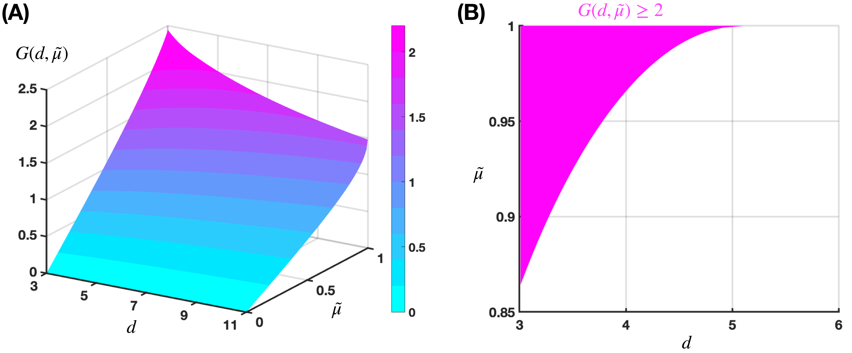
Figure 1: Our numerical investigation for $G(d,\tilde{\mu})$ in Eq. (51). This calculation was done using MatLab R2023a MATLAB . (A) The surface function $G(d,\tilde{\mu})$ inside the region of interests i.e. $(d,\tilde{\mu})\in(3,11]\times[0,1]$. (B) We zoom into the small corner where $G(d,\tilde{\mu})>2$ can be realized. Image taken from Vu2024 .

From Kazuo2019 , above the critical chemical potential when the CSC phase appears, there is a scalar field solution with $J_{c}=0$ and $C\neq 0$. Hence the scalar field near boundary in this case becomes

$$\psi(r)=\frac{C}{r^{d-2}}$$ (53)

Use the variable $z$ we have the second equation of (7) and $r_{+}=1$

$$\begin{split}&\psi^{\prime\prime}(z)+\left[\frac{f^{\prime}(z)}{f(z)}-\frac{d-2}{z}\right]\psi^{\prime}(z)\\ &+\left[\frac{q^{2}\phi^{2}(z)}{f^{2}(z)}-\frac{m^{2}}{f(z)z^{2}}\right]\psi(z)=0\end{split}$$ (54)

From the blackening function (8) we obtain:

$$\frac{f^{\prime}(z)}{f(z)}=\frac{-(d-1)\left(1+\frac{3\mu^{2}}{8}\right)z^{d-2}+\frac{3\mu^{2}}{8}(d+2)z^{d+1}}{1-\left(1+\frac{3\mu^{2}}{8}\right)z^{d-1}+\frac{3\mu^{2}}{8}z^{d+2}}$$ (55)

From the boundary condition (53) we have the form of $\psi(z)$:

$$\psi=Cz^{d-2}H(z)$$ (56)

the function $H(z)$ is trial function and it satisfy the boundary condition $H(0)=1$ and $H^{\prime}(0)=0$. And because this solution is close to the critical chemical potential (above but near), we can consider $\mu\approx\mu_{c}$. We obtain the equation for $H(z)$

$$\begin{split}&H^{\prime\prime}(z)+\frac{f^{\prime}(z)z+(d-2)f(z)}{zf(z)}H^{\prime}(z)\\ &+\frac{(d-2)[f^{\prime}(z)z-f(z)]-m^{2}}{z^{2}f(z)}H(z)\\ &+q^{2}\mu^{2}_{c}\frac{(1-z^{d-3})^{2}}{f^{2}(z)}H(z)=0\end{split}$$ (57)

We rewrite this equation

$$H^{\prime\prime}(z)+p(z)H^{\prime}(z)+q(z)H(z)+\lambda^{2}w(z)\xi^{2}(z)H(z)=0$$ (58)

where $\lambda^{2}=q^{2}\mu_{c}^{2}$ and

$$\begin{split}&p(z)=\frac{f^{\prime}(z)}{f(z)}+\frac{d-2}{z}\\ &q(z)=\frac{d-2}{z}\left(\frac{f^{\prime}(z)}{f(z)}-\frac{1}{z}\right)-\frac{m^{2}}{f(z)z^{2}}\\ &=\frac{(d-2)[-1-d\left(1+\frac{3\mu_{c}^{2}}{8}\right)z^{d-1}+\frac{3\mu_{c}^{2}}{8}(d+1)z^{d+2}]}{[1-\left(1+\frac{3\mu_{c}^{2}}{8}\right)z^{d-1}+\frac{3\mu_{c}^{2}}{8}z^{d+2}]^{2}}\\ &-\frac{m^{2}}{[1-\left(1+\frac{3\mu_{c}^{2}}{8}\right)z^{d-1}+\frac{3\mu_{c}^{2}}{8}z^{d+2}]z^{2}}\\ &w(z)=\frac{1}{f^{2}(z)}=\frac{1}{[1-\left(1+\frac{3\mu_{c}^{2}}{8}\right)z^{d-1}+\frac{3\mu_{c}^{2}}{8}z^{d+2}]^{2}}\\ &\xi^{2}(z)=(1-z^{d-3})^{2}\end{split}$$ (59)

It’s written in form of the Sturm$-$Liuoville equation

$$[T(z)H^{\prime}(z)]^{\prime}-Q(z)H(z)+\lambda^{2}P(z)H(z)=0$$ (60)

where

$$\begin{split}Q(z)&=-T(z)q(z)\\ P(z)&=T(z)w(z)\xi^{2}(z)\\ T(z)&=e^{\int p(z)dz}=f(z)z^{d-2}\\ &=[1-\left(1+\frac{3\mu_{c}^{2}}{8}\right)z^{d-1}+\frac{3\mu_{c}^{2}}{8}z^{d+2}]z^{d-2}\end{split}$$ (61)

From the Sturm$-$Liouville equation, the eigenvalue $\lambda^{2}$ in (60) is obtained by minimizing the following expression

$$\lambda^{2}=\frac{\int_{0}^{1}T(z)H^{\prime 2}(z)dz+\int^{1}_{0}Q(z)H(z)^{2}dz}{\int^{1}_{0}P(z)H^{2}(z)dz}$$ (62)

where the trial function $H(z)$ is chosen as $H(z)=1-az^{2}$ Nam2019 .

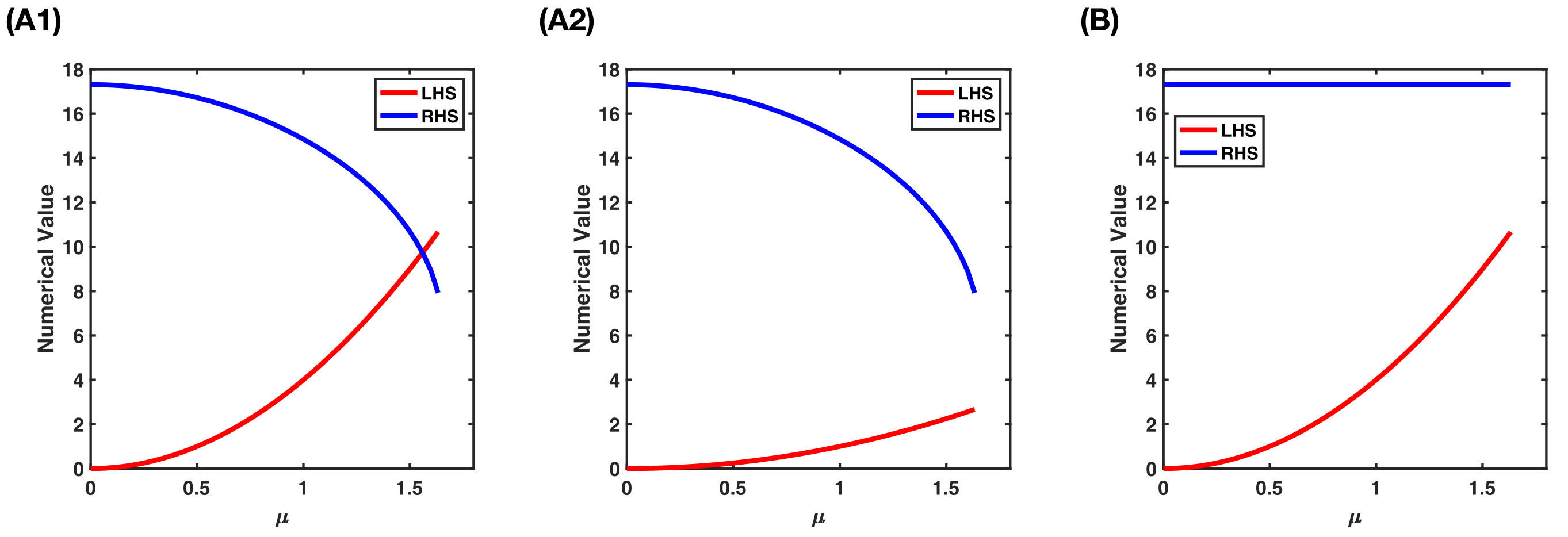
Figure 2: Our numerical investigation for the eigenvalue estimation of the Sturm-Liouville equation. These calculations was done using MatLab R2023a MATLAB , using the test function $H(z)=1-az^{2}$. (A1) Deconfinement phase with $N_{c}=1$, corresponding to Eq. (62). (A2) Deconfinement phase with $N_{c}=2$, corresponding to Eq. (62). (B) Confinement phase with $N_{c}=1$, corresponding to Eq. (72).

With $Nc=1$ we can see that the critical chemical potential exists and $\mu_{c}>1.177$ (see Fig. 2A1). Hence, in the deconfinement phase with $N_{c}=1$, the Einstein$-$Maxwell gravity can study color superconductivity when $d=4$.

But when we solve this equation with $H(z)=1-az^{2}$ and $N_{c}=2$ we don’t see the critical point (see Fig. 2A2), so we can’t obtain this critical chemical potential $\mu_{c}$ with this form of trial function for $N_{c}=2$

However, with $d=4$ if we find one continuous function $H(z)$ that satisfies the RHS of (62) greater than $4\times 1.177$ when $\mu=1.177$ (because we find the CSC phase in the deconfinement phase and we also need to have the CSC phase for both $N_{c}=1$ and $N_{c}=2$) and less than $8/3$ when $\mu=\sqrt{8/3}$, we will confirm that $mu_{c}$ for CSC with $N_{c}=2$ exists. ($H(z)$ is still satisfy $H(0)=1$, and $H^{\prime}(0)=0$). Hence, we have the new conditions of $H(z)$ to obtain CSC with $N_{c}=2$. We can see that in $4$ dimension with $\mu=\sqrt{8/3}$, $f(z,\sqrt{8/3})=1-2z^{3}+z^{6}$ the conditions as follow

$$\begin{split}&\text{RHS}_{f(z)=1-2z^{3}+z^{6}}<8/3\\ &\text{RHS}_{\mu=1.177}>4\times(1.177)^{2}\end{split}$$ (63)

The two conditions in (63) and $H(0)=1$, $H^{\prime}(0)=0$ are all conditions for the trial function $H(z)$ to obtain the CSC phase in the deconfinement phase. If a $H(z)$ that satisfies these conditions exists, we will confirm that the CSC with $N_{c}=2$ when $d=4$ exists. If not we have only CSC phase with $N_{c}=1$ for all dimension in Einstein$-$Maxwell gravity.

If we consider the theory in which the confinement phase not exist Vu2024 . Because it have no confinement phase the chemical potential of deconfinement begin at $\mu=0$. We have the RHS is positive at $\mu=0$ and still less than $8/3$ when $\mu=\sqrt{8/3}$. We have $f(z,0)=1-z^{3}$ hence the condition

$$\begin{split}&\text{RHS}_{f(z)=1-2z^{3}+z^{6}}<8/3\\ &\text{RHS}_{f(z)=1-z^{3}}>0\end{split}$$ (64)

III.2 CSC phase in confinement phase

We now consider for the confinement phase case from (19) we also have the effective mass is

$$m^{2}_{eff}=m^{2}-\frac{q^{2}\phi^{2}(r)}{r^{2}}=m^{2}-\frac{q^{2}\phi^{2}(r)}{r_{0}^{2}}\left(\frac{r_{0}}{r}\right)^{2}$$ (65)

From the BF bound breaking condition (with $r_{0}=1$) we have

$$q^{2}\phi^{2}(r)>\frac{(d-3)^{2}}{4}$$ (66)

Replace the value of $\phi(r)$ in the confinement phase we have

$$q\mu>\frac{d-3}{2}$$ (67)

We obtain

$$N_{c}<\frac{4\mu}{d-3}$$ (68)

We introduce the variable $z=\frac{r_{0}}{r}$ and replace into the second equation of (19) and we set $r_{0}=1$, we have $f(z)=1-z^{d-1}$. After some manipulation which analogy deconfinement case we obtain

$$H^{\prime\prime}(z)+p(z)H^{\prime}(z)+q(z)H(z)+\lambda^{2}w(z)\xi(z)^{2}H(z)=0$$ (69)

where

$$\begin{split}p(z)&=\frac{f^{\prime}(z)}{f(z)}+\frac{d-2}{z}\\ q(z)&=\frac{d-2}{z}\left(\frac{f^{\prime}(z)}{f(z)}-\frac{1}{z}\right)-\frac{m^{2}}{f(z)z^{2}}\\ &=-\left[\frac{d-2}{z}\frac{(d-2)z^{d-1}+1}{z(1-z^{d-1})}+\frac{m^{2}}{z^{2}(1-z^{d-1})}\right]\\ &=-\frac{(d-2)^{2}z^{d-1}+(d-2)+m^{2}}{z^{2}(1-z^{d-1})}\\ w(z)&=\frac{1}{f(z)}\\ \xi(z)&=1\end{split}$$ (70)

And we have the Sturm$-$Liouville form (60) of this equation of motion is

$$\begin{split}Q(z)&=-T(z)q(z)\\ P(z)&=T(z)w(z)\xi^{2}(z)\\ T(z)&=e^{\int p(z)dz}=f(z)z^{d-2}\\ &=[1-z^{d-1}]z^{d-2}\end{split}$$ (71)

The eigenvalue of this equation is calculated by (62) with $H(z)=1-az^{2}$

$$\lambda^{2}=\frac{\int_{0}^{1}T(z)H^{\prime 2}(z)dz+\int^{1}_{0}Q(z)H(z)^{2}dz}{\int^{1}_{0}P(z)H^{2}(z)dz}$$ (72)

We can see that in confinement phase the RHS doesn’t depend on the chemical potential.

By solve the equation (72) with $H(z)=1-az^{2}$ we don’t see the chemical potential in $[0,\sqrt{8/3}]$ to occur the CSC phase transition even with $N_{c}=1$ (see Fig. 2B). Hence in confinement phase the color superconductivity not exist with our trial function $H(z)=1-az^{2}$. If we want to have CSC phase, we need the other form of trial function $H(z)$, still satisfy the condition $H(0)=1$ and H’(0)=0, now we find the condition of $H(z)$ from $N_{c}=1$ to $N_{c}=4$.

To obtain the CSC phase with $N_{c}=1$ in the confinement phase, we need the trial function $H(z)$ that satisfies $H(0)=1$, $H^{\prime}(0)=0$ and

$$\text{RHS}<\frac{4}{N_{c}^{2}}\times(1.177)^{2},$$ (73)

with $N_{c}=1,2,3,4$. If one of $H(z)$ that satisfy these conditions exist we have the CSC phase in the confinement phase with these value of $N_{c}$. If not we have no CSC in the confinement phase.

But the question is what happens if there exist the $H(z)$ which satisfy the condition for $N_{c}\geq 3$ in the deconfinement phase or $N_{c}\geq 5$ in the confinement phase? The answer is the instability condition, this condition does not depend the $H(z)$, this is right for all $H(z)$. Hence, with all $H(z)$, we only have the CSC phase with $N_{c}=2$ in the deconfinement phase, and $N_{c}=4$ in the confinement phase in $d=4$ if we use the Einstein$-$Maxwell gravity.

IV Discussion

We have found that if we only use the Einstein-Maxwell gravity and the standard Maxwell interaction even when $d=4$ it is very difficult to study the CSC phase with $N_{c}=2$. In $d=4$, the confinement$-$deconfiement phase transition occurs when $\mu=1.177$ and the maximum of $\mu$ ($r_{+}=1$) is $\sqrt{8/3}$. When we study the possibility of $N_{c}=2$ CSC phase, we see that in deconfinement phase with $H(z)=1-az^{2}$ it have no $\mu_{c}$ solution, in confinement phase and the same trial function there is no $\mu_{c}$ solution even with $N_{c}=1$. The $N_{c}=2$ critical chemical potential for $N_{c}=2$ CSC only exits if we find one trial function $H(z)$ that satisfy $H(0)=1$, $H^{\prime}(0)=0$ and the condition (63) for the deconfinement phase and (73) for the confinement phase (or at least we prove that these $H(z)$ which satisfy these condition exist). But with $N_{c}=1$ in deconfinement with simplest $H(z)=1-az^{2}$ we obtained CSC phase. And from Vu2024 we can’t study the CSC phase with $d=3$ (if it occur). This project doesn’t study the energy gap yet, we hope return to study the gap in CSC phase via holography earliest.

The further challenges include developing holographic models for e.g. $p-$wave and $d-$wave CSC, for all confinement and deconfinement phase as well as examining the Josephson junction effect in the CSC phase through holographic QCD, and after we generalized these for an arbitrary $SU(N_{c})$. These aspects are worth exploring in future works.

A compelling avenue for further research involves holographic modeling in fractional dimensions, where the value $d$ varies continuously. As demonstrated in Fig. 1, this framework situates the dual gauge theory in spacetime dimensions below four, opening possibilities for experimental realizations. Advances in fractal lattice design Kempkes2019Design highlight the potential of this direction, given the prevalence of fractional$-$dimensional structures in nature mandelbrot1982fractal . Exploring such models could be particularly impactful for condensed matter and quantum gravity, where these unconventional geometries may uncover novel phenomena, as seen in fluid dynamics phan2024vanishing and soft matter physics phan2020bacterial .

V Acknowledgements

We would like to thank Nam H. Cao for his helpful feedback and insightful discussions. We also acknowledge Trung V. Phan for his assistance in generating Fig. 1, Fig. 2 and editing this manuscript and thank grateful to Dmitry Voskresensky for his valuable discussions on color superconductivity.

References

- (1) Nguyen Hoang Vu. Holographic model for color superconductivity in d-dimension bulk without confinement phase. Physics of Atomic Nuclei, 87, 2024.
- (2) Kazem Bitaghsir Fadafan, Jesus Cruz Rojas, and Nick Evans. Holographic description of color superconductivity. Physical Review D, 98(6):066010, 2018.
- (3) Kazem Bitaghsir Fadafan, Jesús Cruz Rojas, and Nick Evans. Holographic quark matter with color superconductivity and a stiff equation of state for compact stars. Physical Review D, 103(2):026012, 2021.
- (4) B.P.Abbott et al. Gw170817: Obeservation of gravitational waves from a binary neutron star inspiral. Phys.Rev.Lett 119 161101, 2017.
- (5) Juan Maldacena. The large-n limit of superconformal field theories and supergravity. International journal of theoretical physics, 38(4):1113–1133, 1999.
- (6) Edward Witten. Anti de sitter space and holography. arXiv preprint hep-th/9802150, 1998.
- (7) Steven S Gubser, Igor R Klebanov, and Alexander M Polyakov. Gauge theory correlators from non-critical string theory. Physics Letters B, 428(1-2):105–114, 1998.
- (8) Trung V Phan and Anh Doan. A curious use of extra dimension in classical mechanics: Geometrization of potential. J. Geom. Graphics, 25:265–270, 2021.
- (9) Pallab Basu, Fernando Nogueira, Moshe Rozali, Jared B Stang, and Mark Van Raamsdonk. Towards a holographic model of color superconductivity. New Journal of Physics, 13(5):055001, 2011.
- (10) Anastasia A Golubtsova and Vu H Nguyen. Wilson loops in exact holographic rg flows at zero and finite temperatures. Theoretical and Mathematical Physics, 202(2):214–230, 2020.
- (11) Sean A Hartnoll, Christopher P Herzog, and Gary T Horowitz. Building a holographic superconductor. Physical Review Letters, 101(3):031601, 2008.
- (12) Sean A Hartnoll, Christopher P Herzog, and Gary T Horowitz. Holographic superconductors. Journal of High Energy Physics, 2008(12):015, 2008.
- (13) Cao H Nam. Holographic model with power-law maxwell field for color superconductivity. Physical Review D, 106(12):126021, 2022.
- (14) Kazuo Ghoroku, Kouji Kashiwa, Yoshimasa Nakano, Motoi Tachibana, and Fumihiko Toyoda. Color superconductivity in a holographic model. Physical Review D, 99(10):106011, 2019.
- (15) Peter Breitenlohner and Daniel Z Freedman. Stability in gauged extended supergravity. Annals of physics, 144(2):249–281, 1982.
- (16) Peter Breitenlohner and Daniel Z Freedman. Positive energy in anti-de sitter backgrounds and gauged extended supergravity. Physics Letters B, 115(3):197–201, 1982.
- (17) Cao H Nam. More realistic holographic model of color superconductivity with higher derivative corrections. Physical Review D, 104(4):046006, 2021.
- (18) Roberto Emparan and Kentaro Tanabe. Holographic superconductivity in the large d expansion. Journal of High Energy Physics, 2014(1):1–22, 2014.
- (19) Cao H Nam. Gauss–bonnet holographic superconductors in exponential nonlinear electrodynamics. General Relativity and Gravitation, 51:1–26, 2019.
- (20) Makoto Natsuume. AdS/CFT duality user guide, volume 903. Springer, 2015.
- (21) O.Miskovic and R.Olea. Quantum statistical relation for black holes in nonlinear electrodynamics coupled to einstein-gauss-bonnet ads gravity. Phys.Rev.D 83 064017, 2011.
- (22) The MathWorks Inc. Matlab version: 9.14.0.2239454 (r2023a), 2023.
- (23) Sander N Kempkes, Marlou R Slot, Saoirsé E Freeney, Stephan JM Zevenhuizen, Daniel Vanmaekelbergh, Ingmar Swart, and C Morais Smith. Design and characterization of electrons in a fractal geometry. Nature physics, 15(2):127–131, 2019.
- (24) Benoit B Mandelbrot. The fractal geometry of nature/revised and enlarged edition. New York, 1983.
- (25) Trung V Phan, Truong H Cai, and Van H Do. Vanishing in fractal space: Thermal melting and hydrodynamic collapse. Physics of Fluids, 36(3), 2024.
- (26) Trung V Phan, Ryan Morris, Matthew E Black, Tuan K Do, Ke-Chih Lin, Krisztina Nagy, James C Sturm, Julia Bos, and Robert H Austin. Bacterial route finding and collective escape in mazes and fractals. Physical Review X, 10(3):031017, 2020.