Multiresolution relaxation times

lattice Boltzmann schemes with projection

François Dubois^ab and Paulo Cesar Philippi^c

^a Laboratoire de Mathématiques d’Orsay, Faculté des Sciences d’Orsay,

Université Paris-Saclay, France.

^b Conservatoire National des Arts et Métiers, LMSSC laboratory, Paris, France.

^c Pontifícia Universidade Católica do Paraná, Curitiba, Paraná, Brazil.

20 December 2024

Keywords: partial differential equations, asymptotic analysis

AMS classification: 76N15, 82C20.

PACS numbers: 02.70.Ns, 47.10.+g

Abstract

We propose to extend the multiresolution relaxation times lattice Boltzmann schemes with a additional projection step. For the explicit example of the D2Q9 scheme, we define this extended method. We prove that in general the projection step does not change the asymptotic partial differential equations at second order. We present four numerical test cases. One concerns linear stability with a Fourier analysis with a single-vertex scheme. Three bidimensional fluid flows with a coarse mesh have been tested: the Minion and Brown sheared flow, the Ghia, Ghia and Shin lid-driven cavity and an unsteady acoustic wave. Our results indicate that the bulk viscosity can be dramatically reduced with a better stability than the initial scheme.

1)  Introduction

The single relaxation time lattice Boltzmann schemes proposed by Higuera and Jiménez [24], McNamara and Zanetti [34], Qian, d’Humières and Lallemand [41] have two origins: the lattice gas automata of Hardy, Pomeau and de Pazzis [21] and Frisch, Hasslacher and Pomeau [16], and the discrete velocities models for the Boltzmann equation introduced by Carleman [8], Broadwell [7], and Gatignol [17].

The multiresolution relaxation times (MRT) lattice Boltzmann scheme is essentially due to d’Humières [26]. Two representations of the discrete gas are used: a particle representation and a representation of the state with set of moments. The macroscopic moments are conserved during the collision and satisfy asymptotically a set of macroscopic partial differential equations. The non-equilibrium moments are not conserved and relax towards an equilibrium function using several relaxation times. This method is well understood since the work of Lallemand and Luo [30].

In a remarkable 1994 paper, Ladd [29] introduced two new ingredients in writing athermal second-order LB equations. First, the collision operator was linearized giving rise to a kinetic model written in terms of second-order moments, with two independent collision frequencies. Second, the relaxation of the viscous stress tensor was decomposed into the relaxation of its deviatoric and isotropic parts.

A new idea has been proposed by Shan et al. [43] and Philippi et al. [40] with the introduction of Hermite polynomials to represent the moments at equilibrium. A simplification of the method, so-called “regularization” has been proposed by Latt and Chopard [31]. The recursivity and regularization of Malaspinas [33] is an extension of Latt’s algorithm. The high-order regularization of Mattila et al. [37] is the basis of developments done by one of us. The initial MRT algorithm is simplified and the number of parameters is reduced. But it is necessary to have a good knowledge of the algebraic properties of the Hermite polynomials and their links with transport properties of fluids.

In this contribution, we follow a totally discrete approach without any need of Hermite polynomials. The Taylor expansion method [12] has been extended with the introduction of the differential advection operator in the basis of moments and the “ABCD” decomposition [13]. Then the analysis of MRT lattice Boltzmann schemes can be conducted without any a priori reference to fluid properties. The equivalent partial differential equations can be formally derived from the knowledge of the equilibrium value of the non-equilibrium moments and the relaxation parameters.

We have observed in [15] that three families of moments emerge from the asymptotic analysis of lattice Boltzmann schemes: the conserved moments $W$ that define the unknowns of the equivalent partial differential equations, the nonconserved “viscous moments” $Y_{e}$ for setting the first order terms and the nonconserved “energy transfer moments” $Y_{v}$ for adjusting second-order dissipation. Precise definitions of these quantities are given below.

In this contribution, we propose a new “multiresolution relaxation times with projection” lattice Boltzmann scheme inspired by kinetic regularization involving Hermite polynomials (see e.g. [31, 33, 37] and many others!). Our motivation is to be able to make the computations very near the stability limit. In that case, the use of a coarse mesh is possible and the global cost of the computation is reduced.

The outline of our contribution is the following. We remind in section 2 the essential about the multiple relaxation time schemes for fluids, in particular for the D2Q9 lattice Boltzmann scheme. Then in section 3, we explain how the equivalent partial equivalent differential equations emerge from an asymptotic analysis based on the ABCD decomposition. The present projected multiple relaxation time D2Q9 scheme is presented in section 4. We insist on the importance of the hollow structure of the matrix of advection in the basis of moments. The asymptotic analysis of the MRT scheme with projection is conducted in section 5. The first numerical experiments for a linear model problem are presented in section 6. In section 7, we focus on two fluid applications for two space dimensions. An unsteady linear acoustics problem is presented in section 8. Some words of conclusion are proposed in section 9. The section 10 is an appendix developing a technical point relative to the multiresolution relaxation times lattice Boltzmann schemes with projection.

2)  Multiple relaxation time D2Q9 scheme for fluids

In this section, we recall the basics about the D2Q9 lattice Boltzmann scheme for isothermal fluid flow, studied in detail by Lallemand and Luo [30]. Recall that in the MRT framework proposed by d’Humières [26], the mesoscopic scale is represented with the vector $\,f\,$ describing the distribution of particle populations over the discrete set $\,e_{j}\,$ for $\,j=0,\dots,b-1\,$ of microscpîc velocities, and the vector $\,m\,$ of moments. The vector of particles is associated to a velocity rose described on a square lattice at the Figure 1. A scale speed $\,\lambda\,$ is associated to the ratio between the space step $\,\Delta x\,$ and the time step $\,\Delta t$:

$$\lambda={{\Delta x}\over{\Delta t}}\,.\vspace*{-6pt}$$

Figure 1: The nine velocities of the D2Q9 scheme [30].

The velocities $\,e_{j}\,$ for $\,0\leq j\leq b\equiv 8\,$ of the D2Q9 scheme described in Figure 1 admit the components $\,e_{jx},e_{jy}$. They are scaled with the numerical velocity $\,\lambda$. We have

$$\{e_{j}\}=\begin{pmatrix}0&\lambda&0&-\lambda&0&\lambda&-\lambda&-\lambda&\lambda\\ 0&0&\lambda&0&-\lambda&\lambda&\lambda&-\lambda&-\lambda\end{pmatrix}\,.\vspace*{-6pt}$$

The particles and the moments are linked together with the “d’Humières matrix” $\,M\,$ such that

$$m=M\,f\,.\vspace*{-7pt}$$ (1)

Following [30], the matrix $\,M\,$ is constructed with the help of polynomials relative to the velocities $\,e_{i}$. We have

$$M_{ij}=P_{i}(e_{jx},e_{jy})\vspace*{-6pt}$$

with a family of polynomials given in [30] by

$$\left\{\begin{array}[]{rcl}P_{0}(e_{jx},e_{jy})&=&1\\ P_{1}(e_{jx},e_{jy})&=&e_{jx}\\ P_{2}(e_{jx},e_{jy})&=&e_{jy}\\ P_{3}(e_{jx},e_{jy})&=&3\,(e_{jx}^{2}+e_{jy}^{2})-4\,\lambda^{2}\\ P_{4}(e_{jx},e_{jy})&=&e_{jx}^{2}-e_{jy}^{2}\\ P_{5}(e_{jx},e_{jy})&=&e_{jx}\,e_{jy}\\ P_{6}(e_{jx},e_{jy})&=&\big{[}3\,(e_{jx}^{2}+e_{jy}^{2})-5\,\lambda^{2}\big{]}\,e_{jx}\\ P_{7}(e_{jx},e_{jy})&=&\big{[}3\,(e_{jx}^{2}+e_{jy}^{2})-5\,\lambda^{2}\big{]}\,e_{jy}\\ P_{8}(e_{jx},e_{jy})&=&{9\over 2}\,(e_{jx}^{2}+e_{jy}^{2})^{2}-{21\over 2}\,(e_{jx}^{2}+e_{jy}^{2})+4\,\lambda^{4}\end{array}\right.\,.\vspace*{-6pt}$$

The matrix $\,M\,$ is an invertible fixed matrix. Following [30], its lines are chosen orthogonal and each line corresponds to a specific moment. We have for the D2Q9 scheme:

$$M=\left[\!\!\begin{array}[]{ccccccccc}1\!&\!1\!&\!1\!&\!1\!&\!1\!&\!1\!&\!1\!&\!1\!&\!1\\ 0\!&\!\lambda\!&\!0\!&\!-\lambda\!&\!0\!&\!\lambda\!&\!-\lambda\!&\!-\lambda\!&\!\lambda\\ 0\!&\!0\!&\!\lambda\!&\!0\!&\!-\lambda\!&\!\lambda\!&\!\lambda\!&\!-\lambda\!&\!-\lambda\\ -4\lambda^{2}\!&\!-\lambda^{2}\!&\!-\lambda^{2}\!&\!-\lambda^{2}\!&\!-\lambda^{2}\!&\!2\lambda^{2}\!&\!2\lambda^{2}\!&\!2\lambda^{2}\!&\!2\lambda^{2}\\ 0\!&\!\lambda^{2}\!&\!-\lambda^{2}\!&\!\lambda^{2}\!&\!-\lambda^{2}\!&\!0\!&\!0\!&\!0\!&\!0\\ 0\!&\!0\!&\!0\!&\!0\!&\!0\!&\!\lambda^{2}\!&\!-\lambda^{2}\!&\!\lambda^{2}\!&\!-\lambda^{2}\\ 0\!&\!-2\lambda^{3}\!&\!0\!&\!2\lambda^{3}\!&\!0\!&\!\lambda^{3}\!&\!-\lambda^{3}\!&\!-\lambda^{3}\!&\!\lambda^{3}\\ 0\!&\!0\!&\!-2\lambda^{3}\!&\!0\!&\!2\lambda^{3}\!&\!\lambda^{3}\!&\!\lambda^{3}\!&\!-\lambda^{3}\!&\!-\lambda^{3}\\ 4\lambda^{4}\!&\!-2\lambda^{4}\!&\!-2\lambda^{4}\!&\!-2\lambda^{4}\!&\!-2\lambda^{4}\!&\!\lambda^{4}\!&\!\lambda^{4}\!&\!\lambda^{4}\!&\!\lambda^{4}\end{array}\!\!\right]\,.\vspace*{-7pt}$$ (2)

In this contribution, the nine moments are represented with the following notations:

$$m=\big{(}\rho,\,J_{x},\,J_{y},\,\varepsilon,\,p_{xx},\,p_{xy},\,q_{x},\,q_{y},\,h\big{)}^{\rm t}.\vspace*{-6pt}$$

We observe that we have by definition $\,p_{xx}=\sum_{j}\big{(}e_{jx}^{2}-e_{jy}^{2}\big{)}\,f_{j}\,$ and $\,p_{xy}=\sum_{j}e_{jx}\,e_{jy}\,f_{j}$. Moreover, following Lallemand and Luo [30], the three moments $\,\varepsilon$, $\,p_{xx}\,$ and $\,p_{xy}\,$ associated with polynomials of degree two define a second-order tensor that describes the transfer of momentum, including the tensor $\,\tau_{\alpha\,\beta}\,$ responsible for the viscous transfer, while $\,q_{x}\,$ and $\,q_{y}\,$ are third-order moments describing the transfer of energy.

The density $\,\rho\,$ and the two components $\,(J_{x},\,J_{y})\,$ of the momentum constitute the vector $\,W\,$ of conserved variables:

$$W=(\rho,\,J_{x},\,J_{y})^{\rm t}\,.\vspace*{-7pt}$$ (3)

The other moments

$$Y=(\varepsilon,\,p_{xx},\,p_{xy},\,q_{x},\,q_{y},\,h)^{\rm t}\vspace*{-7pt}$$ (4)

are the non-equilibrium moments. We have

$$m=\begin{pmatrix}W\\ Y\end{pmatrix}\,.\vspace*{-7pt}$$ (5)

The relaxation process constructs locally a new vector of moments denoted by $\,m^{*}\,$ with a local and nonlinear algorithm. First the conserved moments are invariant in this process:

$$\rho^{*}=\rho,\,J_{x}^{*}=J_{x},\,J_{y}^{*}=J_{y}\vspace*{-6pt}$$

and we have simply $\,W^{*}=W$. Secondly, we define a vector $\,\Phi(W)\,$ of non-conserved moments at equilibrium. We introduce the two components $\,(u,\,v)\,$ of the macroscopic velocity with the relations

$$J_{x}\equiv\rho\ u\,,\,\,J_{y}=\rho\,v.\vspace*{-6pt}$$

For the D2Q9 scheme for fluid flows, we have the classical relations [9, 41]:

$$\left\{\begin{array}[]{rcl}\Phi_{\varepsilon}&=&-2\,\lambda^{2}\,\rho\,+\,3\,\rho\,(u^{2}+v^{2})\\ \Phi_{xx}&=&\rho\,(u^{2}-v^{2})\\ \Phi_{xy}&=&\rho\,u\,v\\ \Phi_{qx}&=&-\rho\,\lambda^{2}\,u\\ \Phi_{qy}&=&-\rho\,\lambda^{2}\,v\\ \Phi_{h}&=&\rho\,\lambda^{4}-3\,\rho\,\lambda^{2}\,(u^{2}+v^{2})\end{array}\right.\vspace*{-7pt}$$ (6)

and

$$\Phi(W)=\big{(}\Phi_{\varepsilon},\,\Phi_{xx},\,\Phi_{xy},\,\Phi_{qx},\,\Phi_{qy},\,\Phi_{h}\big{)}^{\rm t}\,.\vspace*{-7pt}$$ (7)

Then the relaxation operates on the six non-conserved moments and it is parameterized by four “relaxation coefficients” $\,s_{e},\,s_{\mu},\,s_{q},\,s_{h}$. These coefficients characterize the process of relaxation with a family of multiresolution times. We have

$$\left\{\begin{array}[]{rcl}\varepsilon^{*}&=&\varepsilon+s_{\varepsilon}\,(\Phi_{\varepsilon}-\varepsilon)\\ p_{xx}^{*}&=&p_{xx}+s_{\mu}\,(\Phi_{xx}-p_{xx})\\ p_{xy}^{*}&=&p_{xy}+s_{\mu}\,(\Phi_{xy}-p_{xy})\\ q_{x}^{*}&=&{q_{x}}+s_{q}\,(\Phi_{qx}-q_{x})\\ q_{y}^{*}&=&{q_{y}}+s_{q}\,(\Phi_{qy}-q_{y})\\ {h}^{*}&=&{h}+s_{h}\,(\Phi_{h}-{h})\,.\end{array}\right.\vspace*{-7pt}$$ (8)

We write the previous relations in a compact vector form. We first introduce a diagonal matrix containing all the relaxation coefficients:

$$S={\rm diag}\,\big{(}s_{\varepsilon},\,s_{\mu},\,s_{\mu},\,s_{q},\,s_{q},\,s_{h}\big{)}\,.\vspace*{-7pt}$$ (9)

For the approximation “BGK” of the Boltzmann equation initially introduced by Bhatnagar, Gross and Krook [5], all relaxation coefficients are identical.

Then the relations (8) can be written

$$Y^{*}=Y+S\,(\Phi(W)-Y)\,.\vspace*{-7pt}$$ (10)

At the end of the relaxation process, we have constructed the vector $\,m^{*}\,$ of “moments after relaxation”:

$$m^{*}\equiv\begin{pmatrix}W^{*}\\ Y^{*}\end{pmatrix}=\begin{pmatrix}W\\ Y+S\,(\Phi(W)-Y)\end{pmatrix}\vspace*{-6pt}$$

and the vector of equilibria $\,\Phi(W)\,$ is evaluted thanks to the relation (7).

The second step of one iteration of a MRT lattice Boltzmann scheme is the linear advection process. Once the vector $\,m^{*}\,$ of moments after relaxation is define, it is transformed into particles populations:

$$f^{*}=M^{-1}\,m^{*}\,.\vspace*{-6pt}$$

Then these particles are advected with the velocities $\,e_{j}\,$ of the scheme:

$$f_{j}(x,\,t+\Delta t)\,=\,f_{j}^{*}(x-e_{j}\,\Delta t,\,t)\vspace*{-7pt}$$ (11)

which corresponds to the method of characteristics for the advection equation

$${{\partial f_{j}}\over{\partial t}}+e_{j}^{\alpha}\,{{\partial f_{j}}\over{\partial x^{\alpha}}}=0\vspace*{-6pt}$$

when it is exact!

3)  Equivalent partial differential equations

The “ABCD” method for deriving the asymptotic equilavent partial differential equations for the macroscopic moments (Dubois [13]) corresponds to a mathematical reformulation of the discrete multiscale Chapman-Enskog analysis proposed by Alexander et al. [2], McNamara and Alder [35], Qian and Zhou [42], as established in Dubois et al. [14].

We first introduce the advection operator in the basis of moments

$$\Lambda=M\,{\rm diag}\Big{(}\sum_{1\leq\alpha\leq d}e_{\alpha}\,\partial_{\alpha}\Big{)}\,M^{-1}\,.\vspace*{-6pt}$$

For the D2Q9 lattice Boltzmann scheme and the d’Humières matrix $\,M\,$ proposed in Eq. (2), we have

$$\Lambda=\left[\begin{array}[]{|ccc|cccccc|}\hline\cr 0&\!\!\partial_{x}&\!\!\partial_{y}&0&0&\!\!0&\!\!0&0&0\\ {{2\lambda^{2}}\over{3}}\,\partial_{x}&\!\!0&\!\!0&{1\over 6}\,\partial_{x}&{1\over 2}\,\partial_{x}&\!\!\partial_{y}&\!\!0&0&0\\ {{2\lambda^{2}}\over{3}}\,\partial_{y}&\!\!0&\!\!0&{1\over 6}\,\partial_{y}&-{1\over 2}\,\partial_{y}&\!\!\partial_{x}&\!\!0&0&0\\ \vspace{-.4 cm}\hfil&&&&&&&&\\ \hline\cr\vspace{-.4 cm}\hfil&&&&&&&&\\ 0&\!\!\lambda^{2}\,\partial_{x}&\!\!\lambda^{2}\,\partial_{y}&0&0&\!\!0&\!\!\partial_{x}&\partial_{y}&0\\ 0&\!\!{{\lambda^{2}}\over{3}}\,\partial_{x}&\!\!-{{\lambda^{2}}\over{3}}\,\partial_{y}&0&0&\!\!0&\!\!-{1\over 3}\,\partial_{x}&{1\over 3}\,\partial_{y}&0\\ 0&\!\!{{2\,\lambda^{2}}\over{3}}\,\partial_{y}&\!{{2\,\lambda^{2}}\over{3}}\,\partial_{x}&\!\!0&0&\!\!0&\!\!{1\over 3}\,\partial_{y}&\!\!{1\over 3}\,\partial_{x}&0\\ 0&\!\!0&\!\!0&{{\lambda^{2}}\over{3}}\,\partial_{x}&-\lambda^{2}\,\partial_{x}&\!\!\lambda^{2}\,\partial_{y}&\!\!0&0&{1\over 3}\,\partial_{x}\\ 0&\!\!0&\!\!0&{{\lambda^{2}}\over{3}}\,\partial_{y}&\lambda^{2}\,\partial_{y}&\lambda^{2}\,\partial_{x}&\!\!0&0&\!\!{1\over 3}\,\partial_{y}\\ 0&\!\!0&\!\!0&0&0&0&\lambda^{2}\,\partial_{x}&\lambda^{2}\,\partial_{y}&0\\ \hline\cr\end{array}\right]\,.\vspace*{-6pt}$$

This matrix is decomposed into four blocks:

$$\Lambda=\begin{pmatrix}A&B\\ C&D\end{pmatrix}\vspace*{-7pt}$$ (12)

with four matrices $\,A$, $\,B$, $\,C\,$ and $\,D\,$ of differential operators associated to the decomposition proposed in Eq. (5) of the moments:

$$A=\begin{pmatrix}0&\partial_{x}&\partial_{y}\\ {{2\lambda^{2}}\over{3}}\,\partial_{x}&0&0\\ {{2\lambda^{2}}\over{3}}\,\partial_{y}&0&0\end{pmatrix}\,,\quad B=\begin{pmatrix}0&0&0&0&0&0\\ {1\over 6}\,\partial_{x}&{1\over 2}\,\partial_{x}&\partial_{y}&0&0&0\\ {1\over 6}\,\partial_{y}&-{1\over 2}\,\partial_{y}&\partial_{x}&0&0&0\end{pmatrix}\,,\vspace*{-6pt}$$

$$C=\begin{pmatrix}0&\lambda^{2}\,\partial_{x}&\lambda^{2}\,\partial_{y}\\ 0&{{\lambda^{2}}\over{3}}\,\partial_{x}&-{{\lambda^{2}}\over{3}}\,\partial_{y}\\ 0&{{2\,\lambda^{2}}\over{3}}\,\partial_{y}&{{2\,\lambda^{2}}\over{3}}\,\partial_{x}\\ 0&0&0\\ 0&0&0\\ 0&0&0\end{pmatrix}\,,\,\,D=\begin{pmatrix}0&0&0&\partial_{x}&\partial_{y}&0\\ 0&0&0&-{1\over 3}\,\partial_{x}&{1\over 3}\,\partial_{y}&0\\ 0&0&0&{1\over 3}\,\partial_{y}&{1\over 3}\,\partial_{x}&0\\ {{\lambda^{2}}\over{3}}\,\partial_{x}&-\lambda^{2}\,\partial_{x}&\lambda^{2}\,\partial_{y}&0&0&{1\over 3}\,\partial_{x}\\ {{\lambda^{2}}\over{3}}\,\partial_{y}&\lambda^{2}\,\partial_{y}&\lambda^{2}\,\partial_{x}&0&0&{1\over 3}\,\partial_{y}\\ 0&0&0&\lambda^{2}\,\partial_{x}&\lambda^{2}\,\partial_{y}&0\end{pmatrix}\,.\vspace*{-6pt}$$

Then, as remarked in [13], each iteration (11) of the lattice Boltzmann scheme can be expressed as an exact exponential expression:

$$m(x,t+\Delta t)={\rm exp}(-\Delta t\,\Lambda)\,\,m^{*}(x,\,t)\,.\vspace*{-7pt}$$ (13)

In practice, we must consider the development of the exponential of an operator:

$$\exp(-\Delta t\,\Lambda)={\rm I}-\Delta t\,\Lambda+{{\Delta t^{2}}\over{2}}\,\Lambda^{2}+{\rm O}(\Delta t^{3})\,.\vspace*{-6pt}$$

Moreover, we have to be careful with the non commutation of the product of two matrices, even if all the partial differential operator commute! For example, we have

$$\Lambda^{2}=\Lambda\,\,\Lambda=\begin{pmatrix}A&B\\ C&D\end{pmatrix}\begin{pmatrix}A&B\\ C&D\end{pmatrix}=\begin{pmatrix}A^{2}+B\,C&A\,B+B\,D\\ C\,A+D\,C&C\,B+D^{2}\end{pmatrix}\,.\vspace*{-6pt}$$

With a formal expansion of the evolution into several scales:

$$\partial_{t}=\partial_{t_{1}}+\Delta t\,\partial_{t_{2}}+{\rm O}(\Delta t^{2})\,,\vspace*{-6pt}$$

the Taylor expansion with ABCD method revisit the multiscale Chapman-Enskog. The equivalent partial differential equations of the scheme can be written

$$\left\{\begin{array}[]{l}\partial_{t_{1}}W+\Gamma_{1}=0\\ \partial_{t_{2}}W+\Gamma_{2}=0\\ \Gamma_{1}=A\,W+B\,\Phi(W)\\ Y=\Phi(W)+\Delta t\,S^{-1}\,\Psi_{1}+{\rm O}(\Delta t^{2})\\ \Psi_{1}={\rm d}\Phi(W).\Gamma_{1}-(C\,W+D\,\Phi(W))\\ \Sigma\equiv S^{-1}-{1\over 2}\,{\rm I}\\ \Gamma_{2}=B\,\Sigma\,\Psi_{1}\,.\end{array}\right.\vspace*{-7pt}$$ (14)

In the relations (14), we have introduced the diagonal matrix $\,\Sigma$. This matrix is called the Hénon matrix [23]. For the D2Q9 scheme, we have

$$\Sigma={\rm diag}\,(\sigma_{e},\,\sigma_{\mu},\,\sigma_{\mu},\,\sigma_{q},\,\sigma_{q},\,\sigma_{h})\vspace*{-7pt}$$ (15)

and in particular

$$\sigma_{e}={{1}\over{s_{e}}}-{1\over 2}\,,\,\,\sigma_{\mu}={{1}\over{s_{\mu}}}-{1\over 2}\,.\vspace*{-7pt}$$ (16)

As a reult of the previous asymptotic analysis, the isothermal Navier-Stokes emerge at second order when the third order terms relative to the velocity are neglected (see e.g. [10, 11, 13, 18, 27, 30] and many other references). The asymptotic model satisfies the conservation of mass and momentum:

$$\left\{\begin{array}[]{l}\partial_{t}\rho+\partial_{x}(\rho\,u)+\partial_{y}(\rho\,v)=0\\ \partial_{t}(\rho\,u)+\partial_{x}(\rho\,u^{2}+p)+\partial_{y}(\rho\,u\,v)=\partial_{x}\tau_{xx}+\partial_{y}\tau_{xy}\\ \partial_{t}(\rho\,v)+\partial_{x}(\rho\,u\,v)+\partial_{y}(\rho\,v^{2}+p)=\partial_{x}\tau_{xy}+\partial_{y}\tau_{yy}\,.\end{array}\right.\vspace*{-7pt}$$ (17)

The pressure is given by the relation $\,p=c_{0}^{2}\,\rho\,$ with the speed of sound $\,c_{0}\,$ obtained by the relation $\,c_{0}={{\lambda}\over{\sqrt{3}}}$. The viscous tensor in right hand side of (17) satisfies

$$\left\{\begin{array}[]{l}\tau_{xx}=2\,\mu\,\partial_{x}u+(\zeta-\mu)\,(\partial_{x}u+\partial_{y}v)\\ \tau_{xy}=\mu\,(\partial_{x}v+\partial_{y}u)\\ \tau_{yy}=(\zeta-\mu)(\partial_{x}u+\partial_{y}v)+2\,\mu\,\partial_{y}v\,.\end{array}\right.\vspace*{-6pt}$$

The shear viscosity $\,\mu\,$ satisfies $\,\mu={{\lambda}\over{3}}\,\rho\,\sigma_{\mu}\,\Delta x\,$ and the bulk viscosity $\,\zeta\,$ is given by the relation $\,\zeta={{\lambda}\over{3}}\,\rho\,\sigma_{e}\,\Delta x$.

The preceeding algebraic relations are valid only for two space dimensions. For $\,D\,$ space dimensions, we have

$$\tau_{\alpha\beta}=\mu\,\big{(}\partial_{\alpha}u_{\beta}+\partial_{\beta}u_{\alpha}\big{)}+\Big{(}\zeta-{{2}\over{D}}\,\mu\Big{)}\,({\rm div}\,{\bf u})\,\delta_{\alpha\beta}\vspace*{-6pt}$$

and the trace of the viscous stress is given by $\,\tau_{\alpha\alpha}=\zeta\,D\,({\rm div}\,{\bf u})\,$ with $\,\zeta\,$ the bulk viscosity. Moreover, with the usual definition of viscous stress tensor employed in kinetic theory, where this tensor is interpreted as the macroscopic flux of momentum, a minus sign arises. It differs from the convention used in the Fluid Mechanics theory, where the tensor represents the stress exerted on the fluid by neighboring fluid particles and the minus sign is absent.

We observe that the equilibrium value of the viscous moments $\,\varepsilon,\,p_{xx},\,p_{xy}\,$ fix perfect fluid terms. For this reason, the vector $\,Y_{e}\,$ of viscous moments is defined by

$$Y_{e}=\begin{pmatrix}\varepsilon\\ p_{xx}\\ p_{xy}\end{pmatrix}.\vspace*{-7pt}$$ (18)

In a similar way, the equilibrium value of the energy transfer moments $\,q_{x},\,q_{y}\,$ allow adjustment of second-order terms. In this contribution, the energy transfer moments $\,Y_{v}\,$ are given according to

$$Y_{v}=\begin{pmatrix}q_{x}\\ q_{y}\\ h\end{pmatrix}.\vspace*{-7pt}$$ (19)

The expression of the equilibrium of the “ghost moment” $\,h\,$ has been studied by Lallemand and Luo [30], Dellar [10, 11], Geier [18] among others. We observe here that this last moment has no impact on the second order equations (17).

4)  Projected multiple relaxation time D2Q9 scheme

Following the remark done at the end of the previous section, we replace the family $\,Y\,$ of non-conserved moments by two families $\,Y_{e}\,$ and $\,Y_{v}\,$ with $\,Y=(Y_{e},\,Y_{v})^{\rm t}$. The important point concerns the advection operator $\,\Lambda\,$ in the basis of moments. For isothermal D2Q9 studied in the previous section, the operator $\,\Lambda\,$ contains a certain number of zero blocks, as observed therehein:

$$\Lambda=\left[\begin{array}[]{|ccc|ccc|ccc|}\hline\cr 0&\!\!\partial_{x}&\!\!\partial_{y}&0&0&\!\!0&\!\!0&0&0\\ {{2\lambda^{2}}\over{3}}\,\partial_{x}&\!\!0&\!\!0&{1\over 6}\,\partial_{x}&{1\over 2}\,\partial_{x}&\!\!\partial_{y}&\!\!0&0&0\\ {{2\lambda^{2}}\over{3}}\,\partial_{y}&\!\!0&\!\!0&{1\over 6}\,\partial_{y}&-{1\over 2}\,\partial_{y}&\!\!\partial_{x}&\!\!0&0&0\\ \vspace{-.4 cm}\hfil&&&&&&&&\\ \hline\cr\vspace{-.4 cm}\hfil&&&&&&&&\\ 0&\!\!\lambda^{2}\,\partial_{x}&\!\!\lambda^{2}\,\partial_{y}&0&0&\!\!0&\!\!\partial_{x}&\partial_{y}&0\\ 0&\!\!{{\lambda^{2}}\over{3}}\,\partial_{x}&\!\!-{{\lambda^{2}}\over{3}}\,\partial_{y}&0&0&\!\!0&\!\!-{1\over 3}\,\partial_{x}&{1\over 3}\,\partial_{y}&0\\ 0&\!\!{{2\,\lambda^{2}}\over{3}}\,\partial_{y}&\!{{2\,\lambda^{2}}\over{3}}\,\partial_{x}&\!\!0&0&\!\!0&\!\!{1\over 3}\,\partial_{y}&\!\!{1\over 3}\,\partial_{x}&0\\ \vspace{-.4 cm}\hfil&&&&&&&&\\ \hline\cr\vspace{-.4 cm}\hfil&&&&&&&&\\ 0&\!\!0&\!\!0&{{\lambda^{2}}\over{3}}\,\partial_{x}&-\lambda^{2}\,\partial_{x}&\!\!\lambda^{2}\,\partial_{y}&\!\!0&0&{1\over 3}\,\partial_{x}\\ 0&\!\!0&\!\!0&{{\lambda^{2}}\over{3}}\,\partial_{y}&\lambda^{2}\,\partial_{y}&\lambda^{2}\,\partial_{x}&\!\!0&0&\!\!{1\over 3}\,\partial_{y}\\ 0&\!\!0&\!\!0&0&0&0&\lambda^{2}\,\partial_{x}&\lambda^{2}\,\partial_{y}&0\\ \hline\cr\end{array}\right]\,.\vspace*{-6pt}$$

In other terms, we have a 3 by 3 structure composed by six non-zero blocks of 3 by 3 matrices:

$$\Lambda=\begin{pmatrix}A&B_{e}&0\\ C_{e}&0&D_{ev}\\ 0&D_{ve}&D_{vv}\end{pmatrix}\vspace*{-7pt}$$ (20)

with

$$A=\begin{pmatrix}0&\partial_{x}&\partial_{y}\\ {{2\lambda^{2}}\over{3}}\,\partial_{x}&0&0\\ {{2\lambda^{2}}\over{3}}\,\partial_{y}&0&0\end{pmatrix},\,\,B_{e}=\begin{pmatrix}0&0&0\\ {1\over 6}\,\partial_{x}&{1\over 2}\,\partial_{x}&\partial_{y}\\ {1\over 6}\,\partial_{y}&-{1\over 2}\,\partial_{y}&\partial_{x}\end{pmatrix},\,\,C_{e}=\begin{pmatrix}0&\lambda^{2}\,\partial_{x}&\lambda^{2}\,\partial_{y}\\ 0&{{\lambda^{2}}\over{3}}\,\partial_{x}&-{{\lambda^{2}}\over{3}}\,\partial_{y}\\ 0&{{2\,\lambda^{2}}\over{3}}\,\partial_{y}&{{2\,\lambda^{2}}\over{3}}\,\partial_{x}\end{pmatrix},\,\,\vspace*{-6pt}$$

$$D_{ev}=\begin{pmatrix}\partial_{x}&\partial_{y}&0\\ -{1\over 3}\,\partial_{x}&{1\over 3}\,\partial_{y}&0\\ {1\over 3}\,\partial_{y}&{1\over 3}\,\partial_{x}&0\end{pmatrix},\,\,D_{ve}=\begin{pmatrix}{{\lambda^{2}}\over{3}}\,\partial_{x}&-\lambda^{2}\,\partial_{x}&\lambda^{2}\,\partial_{y}\\ {{\lambda^{2}}\over{3}}\,\partial_{y}&\lambda^{2}\,\partial_{y}&\lambda^{2}\,\partial_{x}\\ 0&0&0\end{pmatrix},\,\,D_{vv}=\begin{pmatrix}0&0&{1\over 3}\,\partial_{x}\\ 0&0&{1\over 3}\,\partial_{y}\\ \lambda^{2}\,\partial_{x}&\lambda^{2}\,\partial_{y}&0\end{pmatrix}.\vspace*{-6pt}$$

In consequence, it is natural to propose a new structure for the moments with three components:

$$m=\begin{pmatrix}W\\ Y_{e}\\ Y_{v}\end{pmatrix}.\vspace*{-7pt}$$ (21)

First the conserved moments

$$W=\begin{pmatrix}\rho\\ \rho\,u\\ \rho\,v\end{pmatrix},\vspace*{-7pt}$$ (22)

then the non conserved moments $\,Y\,$ decomposed into two sub-families:

$$Y=\begin{pmatrix}Y_{e}\\ Y_{v}\end{pmatrix}\vspace*{-7pt}$$ (23)

with the Eulerian moments $\,Y_{e}\,$ introduced in (18) and the viscous moments $\,Y_{v}\,$ defined at the relation (19). With this new sub-structure, the non conserved moments at equilibrium can be written

$$\Phi(W)=\begin{pmatrix}\Phi_{e}\\ \Phi_{v}\end{pmatrix}.\vspace*{-6pt}$$

The eulerian moments at equilibrium $\,\Phi_{e}\,$ are obtained with the usual relations (6):

$$\Phi_{e}=\begin{pmatrix}\Phi_{\varepsilon}\\ \Phi_{xx}\\ \Phi_{xy}\end{pmatrix}=\begin{pmatrix}-2\,\lambda^{2}\,\rho\,+\,3\,\rho\,(u^{2}+v^{2})\\ \rho\,(u^{2}-v^{2})\\ \rho\,u\,v\end{pmatrix}\vspace*{-7pt}$$ (24)

and we take for the viscous moments at equilibrium $\,\Phi_{v}\,$ (see again (6)):

$$\Phi_{v}=\begin{pmatrix}\Phi_{qx}\\ \Phi_{qy}\\ \Phi_{h}\end{pmatrix}=\begin{pmatrix}-\rho\,\lambda^{2}\,u\\ -\rho\,\lambda^{2}\,v\\ \rho\,\lambda^{4}-3\,\rho\,\lambda^{2}\,(u^{2}+v^{2})\end{pmatrix}.\vspace*{-7pt}$$ (25)

The defect of equilibrium $\,\Psi\,$ is also decomped into two components:

$$\Psi_{1}=\begin{pmatrix}\Psi_{e}\\ \Psi_{v}\end{pmatrix}.\vspace*{-7pt}$$ (26)

Recall that the Hénon matrix $\,\Sigma\,$ is defined according to

$$\Sigma=S^{-1}-{1\over 2}\,{\rm I}.\vspace*{-7pt}$$ (27)

This diagonal matrix is now considered as decomposed into two blocks:

$$\Sigma={\rm diag}\,\big{(}\,\Sigma_{e}\,,\,\Sigma_{v}\,\big{)}\vspace*{-7pt}$$ (28)

and the first block $\,\Sigma_{e}\,$ is a diagonal 3 by 3 matrix:

$$\Sigma_{e}={\rm diag}\,(\sigma_{e},\,\sigma_{\mu},\,\sigma_{\mu}).\vspace*{-7pt}$$ (29)

with $\,\sigma_{e}\,$ and $\,\sigma_{\mu}\,$ specified in relation (16).

5)  Asymptotic analysis of the MRT scheme with projection

We first revisit the classic MRT scheme when the struture emerging in relations (20)-(29) is taken into account. With this choice of a substruture, and in particular the advection matrix in the basis of moments given according to the block decomposition (20), the equivalent partial differential equations of the second order of the MRT scheme described by the relations (14) take the form

$$\left\{\begin{array}[]{l}\partial_{t_{1}}W+\Gamma_{1}=0\\ \Gamma_{1}=A\,W+B_{e}\,\Phi_{e}(W)\\ Y_{e}=\Phi_{e}(W)+\Delta t\,S_{e}^{-1}\,\Psi_{e}+{\rm O}(\Delta t^{2})\\ \Psi_{e}={\rm d}\Phi_{e}(W).\Gamma_{1}-(C_{e}\,W+D_{ev}\,\Phi_{v}(W))\\ \Sigma_{e}={\rm diag}(\sigma_{e},\,\sigma_{\mu},\,\sigma_{\mu})\\ \Gamma_{2}=B_{e}\,\Sigma_{e}\,\Psi_{e}\\ \partial_{t_{2}}W+\Gamma_{2}=0\,.\end{array}\right.\vspace*{-7pt}$$ (30)

First observe that the relations (30) are completely equivalent to the initial system (14). This property can be demonstrated as follows. We have from (14) the relation $\,\partial_{t_{1}}W+\Gamma_{1}=0$. Then the following calculus

$$\Gamma_{1}=A\,W+B\,\Phi(W)=A\,W+B_{e}\,\Phi_{e}(W)\vspace*{-6pt}$$

establishes the first order relations in (30). For the nonconserved moments, the relation $\,Y=\Phi(W)+\Delta t\,S^{-1}\,\Psi_{1}+{\rm O}(\Delta t^{2})\,$ is splitted into two components according to (23). For the first component, we have $\,Y_{e}=\Phi_{e}(W)+\Delta t\,S_{e}^{-1}\,\Psi_{e}+{\rm O}(\Delta t^{2})$. Now, the two sub-vectors decomposition (26) introduces a first component $\,\Psi_{e}$. from the structure (20), we deduce

$$\Psi_{e}={\rm d}\Phi_{e}(W).\Gamma_{1}-(C_{e}\,W+D_{ev}\,\Phi_{v}(W)).\vspace*{-6pt}$$

Then, due to the substructuring of the Hénon matrix, we have (28)

$$\Gamma_{2}=B\,\Sigma\,\Psi_{1}=B_{e}\,\Sigma_{e}\,\Psi_{e}\vspace*{-6pt}$$

and the set of relations (30) is established. $\square$

We observe now that, as previously observed in [31, 33, 37] in an other context, the equilibria (25) are related to the equilibria (24) according to the relation

$$\Phi_{v}=K\,W+L\,\Phi_{e}\vspace*{-7pt}$$ (31)

with

$$K=\begin{pmatrix}0&-\lambda^{2}&0\\ 0&0&-\lambda^{2}\\ -\lambda^{4}&0&0\end{pmatrix}\,,\quad L=\begin{pmatrix}0&0&0\\ 0&0&0\\ -\lambda^{2}&0&0\end{pmatrix}\,.\vspace*{-7pt}$$ (32)

The relation (31) has been inspired by the recurrence relations between Hermite polynomials, developed in Malaspinas [33] and Mattila et al. [37]. Observe that we have simply

$$\left\{\begin{array}[]{l}-\rho\,\lambda^{2}\,u=-\lambda^{2}\,(\rho\,u)\\ -\rho\,\lambda^{2}\,v=-\lambda^{2}\,(\rho\,v)\\ \rho\,\lambda^{4}-3\,\rho\,\lambda^{2}\,(u^{2}+v^{2})=-\lambda^{4}\,\rho-\lambda^{2}\,\big{(}-2\,\lambda^{2}\,\rho\,+\,3\,\rho\,(u^{2}+v^{2})\big{)}\end{array}\right.\vspace*{-6pt}$$

and the relation (31) is a simple consequence of (24) and (25). $\square$

In conclusion of this important remark, we have obtained with (31) a simple expression of the viscous moments at equilibrium $\,\Phi_{v}\,$ with a linear expression of the conserved variables $\,W\,$ and the eulerian moments $\,\Phi_{e}$.

From the previous remark, we define a projection operator $\,P\,$ in the space of moments by the relation

$$P\,\begin{pmatrix}W\\ Y_{e}\\ Y_{v}\end{pmatrix}=\begin{pmatrix}W\\ Y_{e}\\ K\,W+L\,Y_{e}\end{pmatrix}\vspace*{-7pt}$$ (33)

with the help of the two matrices $\,K\,$ and $\,L\,$ introduced at the relation (32). The projected vector $\,Pm\,$ has three compoents:

$$\left\{\begin{array}[]{l}(Pm)_{W}=W\\ (Pm)_{e}=Y_{e}\\ (Pm)_{v}=K\,W+L\,Y_{e}\,.\end{array}\right.\vspace*{-7pt}$$ (34)

With this projector operator, we define a multiple relaxation time lattice Boltzmann scheme with projection by the following algorithm. For a set of moments $\,m\,$ given by the relation (21) for the D2Q9 lattice Boltzmann scheme, we have

(i)   projection of the moments $\,m\longrightarrow Pm$.

Then the moments at equilibrium $\,(Pm)^{\rm eq}\,$ can be decomposed into three vector components:

$$(Pm)^{\rm eq}=\begin{pmatrix}W\\ \Phi_{e}\\ K\,W+L\,\Phi_{e}\end{pmatrix}=\begin{pmatrix}W\\ \Phi_{e}\\ \Phi_{v}\end{pmatrix}=m^{\rm eq}\vspace*{-7pt}$$ (35)

(ii)  relaxation $\,Pm\longrightarrow(Pm)^{*}$.

We have simply

$$(Pm)^{*}=\begin{pmatrix}W\\ Y_{e}^{*}\\ K\,W+L\,Y_{e}^{*}\end{pmatrix}\vspace*{-7pt}$$ (36)

with $\,Y_{e}^{*}=({\rm I}-S_{e})\,Y_{e}+S_{e}\,\Phi_{e}$. We observe that we have now

$$Y_{v}^{*}=K\,W+L\,Y_{e}^{*}\vspace*{-7pt}$$ (37)

instead of $\,Y_{v}^{*}=({\rm I}-S_{v})\,Y_{v}+S_{v}\,\Phi_{v}\,$ for the initial lattice Boltzmann scheme.

(iii)  propagation

From the moments after relaxation, we introduce the particle representation

$$f^{*}=M^{-1}(Pm)^{*}.\vspace*{-7pt}$$ (38)

This distribution is exactly advected during one time step:

$$f_{j}(x,\,t+\Delta t)\,=\,f_{j}^{*}(x-e_{j}\,\Delta t,\,t)\,.\vspace*{-7pt}$$ (39)

The moments $\,m\,$ at the new time step are a linear transform of the particles: $\,m=M\,f$. Then the algorith can be iterated again.

The MRT lattice Boltzmann scheme with projection has the same asymptotic properties at second order than the initial multiresolution relaxation times lattice Boltzmann scheme. An important result of our contribution is the following

Proposition 1 : a theoretical result for the MRT scheme with projection

For the MRT scheme with projection defined at the relations (33) to (39), we have at second order the following set of partial differential equations

$$\left\{\begin{array}[]{l}\partial_{t}W+\Gamma_{1}+\Delta t\,\Gamma_{2}={\rm O}(\Delta t^{2})\\ \Gamma_{1}=A\,W+B_{e}\,\Phi_{e}\\ \Psi_{e}={\rm d}\Phi_{e}(W).\Gamma_{1}-(C_{e}\,W+D_{ev}\,\Phi_{v}(W))\\ \Gamma_{2}=B_{e}\,\Sigma_{e}\Psi_{e}\,.\end{array}\right.\vspace*{-7pt}$$ (40)

At second order of accuracy, the MRT scheme with projection represents the same physics than the initial MRT scheme.

The proof of this result is developed in Annex 1.

We observe that the resulting model (40) is identical to the result (30) for initial multiresolution relaxation times lattice Boltzmann scheme. The projection step does not change the asymptotic physical model at second order!

We observe finally that the preceding proposition is general in scope. Nevertheless, we consider in this contribution the MRT scheme with projection only for the D2Q9 lattice Boltzmann scheme. If the advection matrix operator in the basis of moments $\,\Lambda\,$ admits a structure of the type (20), the equivalent partiel differential equations satisfy the Proposition 1 and in particular the relations (40). The projected MRT scheme is derived following a general algorithm. The hypothesis is essentially that the matrix of advection in the basis of moments admits a block structure of the type (12) and that the moments at equilibrium verify an identity of the type (31)

6)  Numerical experiments for a linear model

We have implemented the algorithm (33)-(39) for the D2Q9 scheme. Our first results concern a linearized version of the D2Q9 scheme around a constant state with velocity

$$(u_{0},\,v_{0})=(0.2,\,0)\vspace*{-6pt}$$

and sound velocity $\smash{c_{0}={{1}\over{\sqrt{3}}}}$. We have in that case a linearization of the scheme (24)(25)

$$W=\begin{pmatrix}\rho\\ \rho\,(u_{0}+u)\\ \rho\,v\end{pmatrix},\,\,\Phi_{e}(W)=\begin{pmatrix}-2\,\lambda^{2}\,\rho\,+\,6\,\rho\,u_{0}\,u\\ 2\,\rho\,u_{0}\,u\\ 0\end{pmatrix},\,\,\Phi_{v}(W)=\begin{pmatrix}-\rho\,\lambda^{2}\,(u_{0}+u)\\ -\rho\,\lambda^{2}\,v\\ \rho\,\lambda^{4}-6\,\rho\,\lambda^{2}\,u_{0}\,u\end{pmatrix}.\vspace*{-6pt}$$

We can verify very simply that the matrices $\,K\,$ and $\,L\,$ introduced in (32) satisfy the relation (31): we have $\,\Phi_{v}=K\,W+L\,\Phi_{e}$.

For each set of parameters ($s_{\mu}$, $\,s_{e}$), we determine the maximum values of the associated aigenvalues for all the wave vectors, following the method proposed in Lallemand and Luo [30]. If the maximum of moduli of these eigenvalues is greater than one, the scheme is unstable. The iso-maxima of the eigenvalues are represented in Figure 2. They show a significant increase in the stability zone for the relaxation parameter $\,s_{e}$. With the initial MRT scheme, stability is limited to the range $\,0\leq s_{e}\leq 1.75$. The projected MRT lattice Boltzmann scheme is stable for $\,0\leq s_{e}\leq 2\,$ and $\,0\leq s_{\mu}\leq 1.9$.

 

Figure 2: Comparison of linear stability zones for advection speed $u_{0}=0.35\,c_{0}$ and $\,v_{0}=0$. Traditional D2Q9 scheme [30] on the left and D2Q9 MRT with projection on the right. The stability zone is extended for higher values of the relaxation parameter $\,s_{e}$.

7)  Numerical tests for fluid applications

We have first considered two classical test cases: the Minion-Brown test case [38] studying the performance of under-resolved two-dimensional incompressible flow simulations, and the lid-driven cavity proposed by Ghia et al. [19]

The Minion-Brown test case describes a Kelvin-Helmholtz instability. At the initial time, the density is constant and the velocity is given in the square $\,[0,\,L]^{2}\,$ with $\,L=1\,$ by the relations

$$u=\left\{\begin{array}[]{l}\tanh\big{[}\kappa\,\big{(}y-{1\over 4}\big{)}\big{]}\,\,{\rm{for}}\,\,y\leq{1\over 2}\\ \tanh\big{[}\kappa\,\big{(}{3\over 4}-y\big{)}\big{]}\,\,{\rm{for}}\,\,y\geq{1\over 2}\end{array}\right.,\,\,v=\delta\,\sin\Big{[}2\pi\big{(}x+{1\over 4}\big{)}\Big{]}\vspace*{-7pt}$$ (41)

with

$$\kappa=80\,,\,\,\delta=0.05\,.\vspace*{-6pt}$$

This test case has been simulated with the help of lattice Boltzmann schemes by Marié et al. [36], Dellar [11] and Mattila et al. [37] among others.

We first explain how we have chosen our numerical parameters. As proposed in [38], a relative coarse mesh is used and all our compuatations have been done with

$$N=128\vspace*{-6pt}$$

mesh points in each direction. Then $\,\Delta x={{1}\over{N}}=0.0078125$. We have chosen the same Mach number $\,M_{0}\equiv{{U_{0}}\over{c_{0}}}=0.04\,$ as in reference [36]. With the classical value $\,c_{0}={{1}\over{\sqrt{3}}}\,$ for the sound velocity, we have a reference velocity $\,U_{0}=0.0231$. Then with the definition $\,Re\equiv{{U_{0}\,L}\over{\nu}}\,$ of the Reynolds number $\,Re$, we have $\,\nu=2.31\,10^{-6}\,$ when $\,Re=10^{4}$. From the classical relation

$$\nu=\sigma_{\mu}\,{{\Delta x}\over{3}}\vspace*{-7pt}$$ (42)

(see e. g. [30]), we deduce $\,\sigma_{\mu}=8.8704\,10^{-4}\,$ and

$$s_{\mu}={{1}\over{0.5+\sigma_{\mu}}}=1.996458123572134\,.\vspace*{-7pt}$$ (43)

The physical duration is fixed to $\,T={{L}\over{U_{0}}}\approx 43.29$. It corresponds to the final time chosen by Dellar [11]. When $\,\Delta x=\Delta t$, this value can be approximatively translated into

$$N_{T}=5541\vspace*{-7pt}$$ (44)

iterations of the lattice Boltzmann scheme.

Our first simulation concerns the BGK [5] version of the lattice Boltzmann scheme. In that case, all the viscosities are taken identical:

$$s_{e}=s_{q}=s_{h}=s_{\mu}\,.\vspace*{-7pt}$$ (45)

Curiously, our scheme is not diverging with such parameters. But the results (see Figure 3) have nothing to do with what is physically expected!

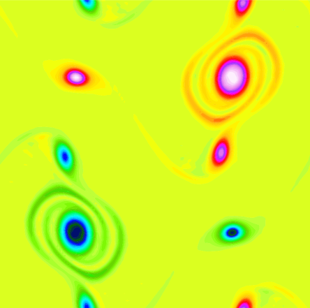
Figure 3: Minion-Brown test case [38] for Reynolds number $\,Re=10^{4}$, 128 grid points and $\,N_{T}=5541\,$ discrete time iterations. BGK results: $\,s_{e}=s_{q}=s_{h}=s_{\mu}$ given by the relation (43). Vorticity field; the results are not satisfying.

 

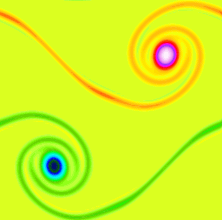
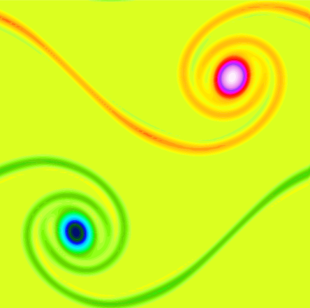
Figure 4: Minion-Brown test case [38] for Reynolds number $\,Re=10^{4}$, 128 grid points and $\,N_{T}\,$ discrete time iterations (44). MRT results on the left with $\,s_{e}=1.715_{,}$ and results for the MRT scheme with projection on the right with the same parameter $\,s_{e}$. These vorticity fields are qualitatively correct.

Then we have taken a MRT scheme with $\,s_{q}=s_{h}=1\,$ to mimic the effects of the projection scheme. With the value $\,s_{e}=1.72$, this MRT scheme is giving overflow values after $\,N_{T}\,$ iterations with the previous parameters. With $\,s_{e}=1.715$, the simulation is giving acceptable results. For this set of parameters, the simulation is close the stability limit for the classic MRT sceme. The results are presented on the left part of the Figure 4. With the MRT lattice Boltzmann scheme with projection, with the same numerical parameters $\,s_{e}\,$ and $\,s_{\mu}$, the computation does not encounter any difficulty. The results are close to the MRT ones and are presented on the right of Figure 4.

It is possible to reduce the bulk viscosity for this Minion and Brown test case with a Reynolds number $\,Re=10^{4}$. With the MRT with projection, we can reduce the bulk viscosity up to $\,\zeta=6.51\,10^{-8}\,$ with $\,s_{e}=1.9999$. The projected MRT lattice Boltzmann scheme remains stable. The Reynolds number based on this bulk viscosity equal to $\,35.5\,10^{4}$. The results are presented in Figure 5.

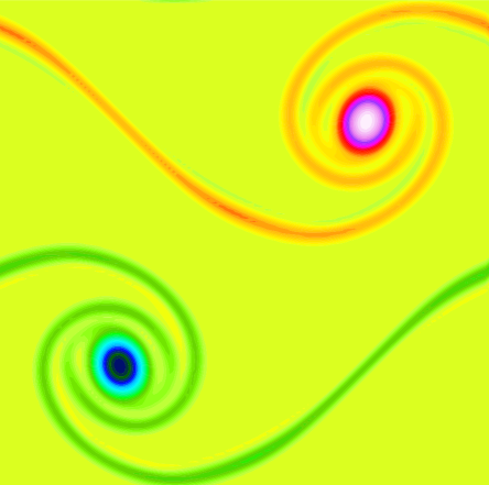
Figure 5: Minion-Brown test case [38] for Reynolds number $\,Re=10^{4}$, 128 grid points and $\,N_{T}=5541\,$ discrete time iterations. Results for the MRT scheme with projection. The bulk viscosity is reduced by using the parameter $\,s_{e}=1.9999$. Vorticity field.

Secondly, we have considered the lid-driven cavity initially proposed by Ghia et al. [19]. This test case has been simulated in the framework of lattice Boltzmann schemes by numerous teams, including Guo et al. [20], Hou et al. [25], Kumar and Agrawal [28], Luo et al. [32], Mohammedi and Reis [39], Hegele et al. [22] and Bazarin et al. [4].

The velocity $\,U_{0}\,$ on the top of the computational domain is taken equal to $\,U_{0}=0.01$. It corresponds to a Mach numer of $\,0.0173$. Then the resulting flow is very close to incompressibility. For this test case, our target Reynolds number is $\,Re=1.000$. We used a mesh with $\,N=128\,$ grid points as in the previous test case. Then from the relation (42), we have $\,\sigma_{\mu}=0.00384\,$ and $\,s_{\mu}=1.984757065735154$.

 

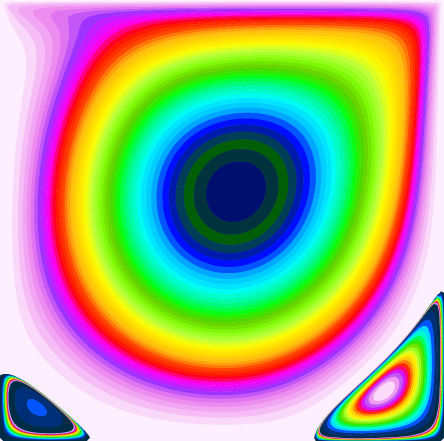
Figure 6: Lid-driven cavity [19] with $Re=1000$ [$s_{\mu}=1.984757065735154$], $s_{e}=1.7$. Stream function for the classic MRT scheme with parameters $s_{q}=s_{h}=1\,$ (left figure) and multiresolution relaxation times scheme with projection (right figure).

 

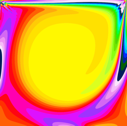
Figure 7: Lid-driven cavity [19] with $Re=1000$ [$s_{\mu}=1.984757065735154$] and $s_{e}=1.98$. Stream function (left figure) and vorticity (right figure) for the MRT scheme with projection.

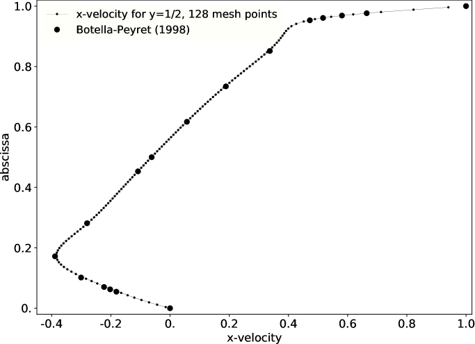
Figure 8: Lid-driven cavity [19] with $Re=1000$ [$s_{\mu}=1.984757065735154$] and $s_{e}=1.98$. MRT scheme with projection: $x$-component of the velocity at $y={1\over 2}\,$ and comparison with Botella and Peyret [6] results.

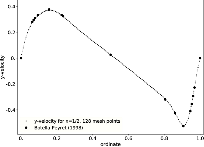
Figure 9: Lid-driven cavity. Same test case than in Figure 8; $y$-component of the velocity at $x={1\over 2}$.

With a relative high value of the bulk viscosity, $\,s_{e}=1.7\,$ to fix the ideas, it has been possible to integrate the initial multiresolution relaxation times scheme with $\,s_{q}=s_{h}=1\,$ up to a stationary solution. We have used $\,N_{T}=400.000\,$ time steps by initializing the velocity field to zero. With the same parameters, the projected multiresolution relaxation times lattice Boltzmann scheme proposes also a stationary fluid flow. They are compared in Figure 6. Observe that taking $\,s_{e}=1.80$, the classic MRT solver is diverging. On the other hand, the projection version gives results that make sense for fluid mechanics. In Figure 7 , we show the results for $\,s_{e}=1.98$, with both the current stream function and the vorticity.

In figures 8 and 9, we present classical outputs for the Ghia et al. test case: the two components of the velocity in the middle of the flow. We compare our results with the reference proposed by Botella and Peyret [6] with a spectral approach.

Our results are quantitavely correct. We consider that these first results validate the multiresolution relaxation times scheme with projection for stationary nearly incompressible fluid flows.

8)  Unsteady linear acoustics

With this test case, we study the two-dimensional propagation of an initial gaussian density profile associated with a zero velocity field. Qualitatively, the evolution is a simple propagation of the disturbance in density at the speed of sound $\,c_{0}={{1}\over{\sqrt{3}}}\simeq 0.5773$. It’s a problem invariant to rotation around the initial center of the Gaussian. This invariance is, of course, broken by any numerical approximation. With this test case, the isotropic qualities and defects of the numerical schemes are particularly highlighted.

We took a number a meshes $\,N=129\,$ in order to have a good location of the mesh center. The initial condition is a gaussian profile for the density:

$$\rho=1+\delta\rho\,\exp\big{(}-r^{2}/R^{2}\big{)}\vspace*{-6pt}$$

with $\,\delta\rho=0.1\,$ and $\,R=0.02$. This gaussian initial condition is represented in figures 10 and 11. We first use a classic MRT scheme with $\,s_{\mu}=1.99$. It corresponds to a Reynolds number $\,Re=88927\,$ based on the speed of sound. We have taken the following relaxation parameters:

$$s_{e}=1.99\,,\,\,s_{q}=1.9\,,\,\,s_{h}=1.54\,.\vspace*{-6pt}$$

The results are shown in figures 12 and 13. The results are globally satisfying. If we want to mimic the projection scheme, we change the two last relaxation parameters for $\,s_{q}=s_{h}=1$. The results are displayed in figures 14 and 15. They clearly indicate than an instability is developing.

With the projection multiresolution relaxation times scheme for the same parameters, id est $\,s_{\mu}=s_{e}=1.99$, the results are very satisfying. We refer to the figures 16 and 17. Rotation invariance is much better satisfied, as shown by the density curve as a function of distance from the center.

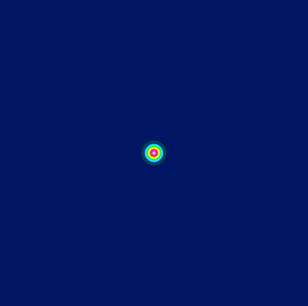
Figure 10: Unsteady acoustics: isovalues of the gaussian initial density

Figure 11: Unsteady acoustics: the gaussian initial density as a function of the radius.

Figure 12: Acoustic with the classic MRT, $s_{\mu}=1.99$, $s_{e}=1.99$, $s_{q}=1.9$, $s_{h}=1.54$, isovalues of the density.

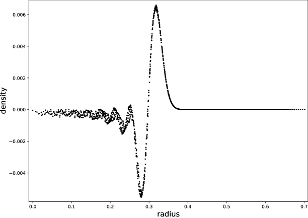
Figure 13: Unsteady acoustics with the classic MRT scheme, $s_{\mu}=1.99$, $s_{e}=1.99$, $s_{q}=1.9$, $s_{h}=1.54$, density as a function of the distance to the center.

Figure 14: Unsteady acoustics with the classic, $s_{\mu}=1.99=s_{e}=1.99$, $s_{q}=s_{h}=1$, isovalues of the density. Strong oscillations are clealy visible.

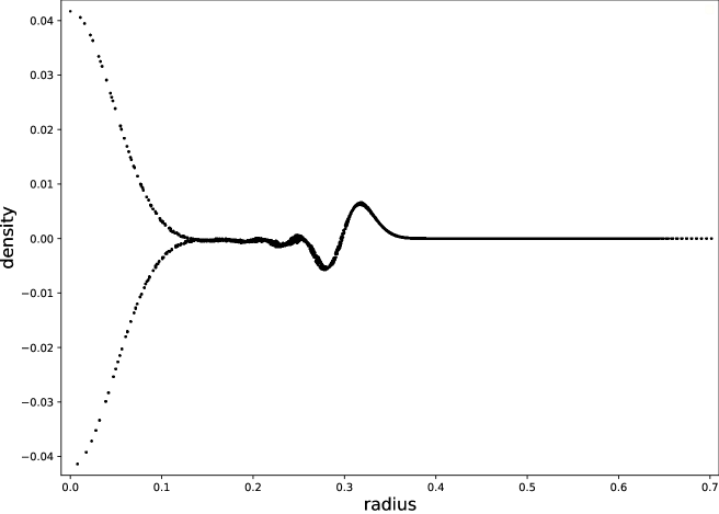
Figure 15: Unsteady acoustics: MRT, $s_{\mu}=1.99=s_{e}=1.99$, $s_{q}=s_{h}=1$, density as a function of the distance to the center.

Figure 16: Unsteady acoustics, MRT with projection with parameters $s_{\mu}=s_{e}=1.99$, isovalues of the density.

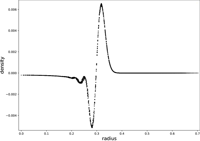
Figure 17: Unsteady acoustics, MRT with projection, $s_{\mu}=s_{e}=1.99$, density as a function of the distance to the center.

Figure 18: Unsteady acoustics: classic MRT scheme with quartic parameters, $s_{\mu}=s_{e}=s_{h}=1.99$, $\sigma_{\mu}\,\sigma_{q}={1\over 6}$. Isovalues of the density.

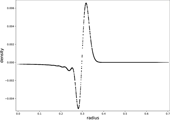
Figure 19: Unsteady acoustics: classic MRT scheme, $s_{\mu}=s_{e}=s_{h}=1.99$, $\sigma_{\mu}\,\sigma_{q}={1\over 6}$, density as a function of the distance to the center.

Last but not least, Augier et al. have studied in [2] the possibility of rotation-invariant MRT lattice Boltzmann schemes up to fourth order. In the D2Q9 case, the “quartic” relaxation parameters take the form

$$\sigma_{\mu}=\sigma_{e}=\sigma_{h}\,,\,\,\sigma_{\mu}\,\sigma_{q}={1\over 6}\,.\vspace*{-6pt}$$

In our case, $\,s_{\mu}=s_{e}=s_{h}=1.99\,$ and the very unusual value $\,s_{q}=0.01496259351620921$. The results are presented in figures 18 and 19. They are very good quality.

As a conclusion of this section, the projected MRT scheme has a very good ability to give correct results with good stability. The initial version of the MRT scheme uses more parameters, is more fragile from a stability point of view, but in some cases produces better quality results.

9)  Conclusion

We have extended the lattice Boltzmann introduced by Malaspinas [33] and developed also by Mattila et al. [37]. Our approach is no longer based on Hermite polynomials of the moments but on the spectific structure (20) of the advection operator in the basis of moments. One advantage of this projection scheme is the reduction in the number of relaxation parameters. Our analysis at second order accuracy shows that the equivalent partial differential equations are not modified by the addition of a projection step in the algorithm. The first numerical tests are satisfying and highlights a gain in stability for the parameters associated to bulk viscosity.

The natural next step is to study lattice Boltzmann schemes in three spatial dimensions. Our results with Pierre Lallemand [15] indicate a favorable block structure for the advection operator in the basis of moments.

10)  Annex: equivalent equations of the projection scheme

We recall the Proposition 1 statement. We suppose that the advection matrix in the basis of moments satisfies the condition (20). We suppose morever that after the decompostion (21) of the moments into conserved variables $\,W$, eulerian moments$\,Y_{e}\,$ and viscous moments $\,Y_{w}$, the equilibrium values satisfy the relation (31). Then the MRT scheme with projection, defined by the relations (33) to (39), satisfies at order two the asymptotic relations (40):

$$\left\{\begin{array}[]{l}\partial_{t}W+\Gamma_{1}+\Delta t\,\Gamma_{2}={\rm O}(\Delta t^{2})\\ \Gamma_{1}=A\,W+B_{e}\,\Phi_{e}\\ \Psi_{e}={\rm d}\Phi_{e}(W).\Gamma_{1}-(C_{e}\,W+D_{ev}\,\Phi_{v}(W))\\ \Gamma_{2}=B_{e}\,\Sigma_{e}\Psi_{e}\,.\end{array}\right.\vspace*{-6pt}$$

We begin by an analysis at order zero. We still have the relation (13)

$$m(x,t+\Delta t)={\rm exp}(-\Delta t\,\Lambda)\,\,m^{*}(x,\,t)\,.\vspace*{-6pt}$$

Moreover, the moments $\,m^{*}\,$ after relaxation satisfy now:

$$m^{*}=(W,\,Y_{e}^{*},\,K\,W+L\,Y_{e}^{*})^{\rm t}\,.\vspace*{-6pt}$$

In consequence, we have $\,m+{\rm O}(\Delta t)=m^{*}+{\rm O}(\Delta x)\,$ and in particular

$$Y_{e}-Y_{e}^{*}\equiv S_{e}\,(Y_{e}-\Phi_{e})={\rm O}(\Delta t)\,.\vspace*{-6pt}$$

Then $\,Y_{e}=\Phi_{e}+{\rm O}(\Delta t)\,$ when $\,S_{e}\,$ is fixed and is invertible. Then we have also

$$Y_{e}^{*}=\Phi_{e}+{\rm O}(\Delta t).\vspace*{-6pt}$$

For the third component, we have due to the relation (37),

$$Y_{v}^{*}\equiv K\,W+L\,Y_{e}^{*}=K\,W+L\,\Phi_{e}+{\rm O}(\Delta t)=\Phi_{v}+{\rm O}(\Delta t)\,.\vspace*{-6pt}$$

We have also $\,(Pm)_{v}+{\rm O}(\Delta t)=Y_{v}^{*}+{\rm O}(\Delta x)\,$ and $\,(Pm)_{v}=\Phi_{v}+{\rm O}(\Delta x)$. Then by combining the three components, we have at order zero

$$m=m^{\rm eq}+{\rm O}(\Delta t)\vspace*{-6pt}$$

and

$$m^{*}=m^{\rm eq}+{\rm O}(\Delta t)\,.\vspace*{-6pt}$$

We consider now the analysis at order one. We expand the relation (13) at first order. For the first component $\,W$, we have

$\,W+\Delta t\,\partial_{t}W+{\rm O}(\Delta t^{2})=W-\Delta t\,(A\,W+B\,Y^{*})+{\rm O}(\Delta t^{2})$

$\,\,\,=W-\Delta t\,(A\,W+B_{e}\,Y_{e}^{*})+{\rm O}(\Delta t^{2})$.

Then we have $\,\partial_{t}W+(A\,W+B_{e}\,Y_{e}^{*})={\rm O}(\Delta t)\,$ and due to the identity $\,Y_{e}^{*}=\Phi_{e}+{\rm O}(\Delta t)$, the relation $\,\partial_{t}W+{\boldsymbol{A}}\,W+B_{e}\,\Phi_{e}(W)={\rm O}(\Delta t)\,$ is still true. In conclusion, we have at first order $\,\Gamma_{1}=A\,W+B_{e}\,\Phi_{e}(W)$.

We consider again now the analysis at order one. We pay attention to the fact that the devil in the details! We expand the relation relation (13) at first order and we focus on the second component. We have

$$Y_{e}+\Delta t\,\partial_{t}Y_{e}+{\rm O}(\Delta t^{2})=Y_{e}^{*}-\Delta t\,(C_{e}\,W+D_{ev}\,Y_{v}^{*})+{\rm O}(\Delta t^{2})\vspace*{-6pt}$$

and we remark that $\,\partial_{t}Y_{e}={\rm d}\Phi_{e}.\partial_{t}W+{\rm O}(\Delta t)=-{\rm d}\Phi_{e}.\Gamma_{1}+{\rm O}(\Delta t)$. Than

$$Y_{e}-\Delta t\,{\rm d}\Phi_{e}.\Gamma_{1}+{\rm O}(\Delta t^{2})=Y_{e}^{*}-\Delta t\,(C_{e}\,W+D_{ev}\,\Phi_{v})+{\rm O}(\Delta t^{2})\,.\vspace*{-6pt}$$

We deduce that $\,\,S_{e}\,(Y_{e}-\Phi_{e})\equiv Y_{e}-Y_{e}^{*}=\Delta t\,[{\rm d}\Phi_{e}.\Gamma_{1}-(C_{e}\,W+D_{ev}\,\Phi_{v})]+{\rm O}(\Delta t^{2})$. With $\,\Psi_{e}={\rm d}\Phi_{e}(W).\Gamma_{1}-(C_{e}\,W+D_{ev}\,\Phi_{v}(W))$, we can expand this family of non-conserved moments at first order: $\,Y_{e}=\Phi_{e}-\Delta t\,S_{e}^{-1}\,\Psi_{e}+{\rm O}(\Delta t^{2})$. Then the relaxation scheme

$$Y_{e}^{*}=({\rm I}-S_{e})\,Y_{e}+S_{e}\,\Phi_{e}\vspace*{-6pt}$$

implies

$Y_{e}^{*}=Y_{e}-S_{e}\,(Y_{e}-\Phi_{e})\,=\Phi_{e}-\Delta t\,S_{e}^{-1}\,\Psi_{e}+\Delta t\,\Psi_{e}+{\rm O}(\Delta t^{2})$

$\,\,\,=\Phi_{e}+\Delta t\,\big{(}{\rm I}-S_{e}^{-1}\big{)}\,\Psi_{e}+{\rm O}(\Delta t^{2})$.

We introduce the “reduced Hénon matrix”

$$\Sigma_{e}\equiv S_{e}^{-1}-{1\over 2}\,{\rm I}\,.\vspace*{-6pt}$$

Then we have the following expansions of the non-conserved moments at first order

$$\left\{\begin{array}[]{l}Y_{e}=\Phi_{e}+\Delta t\,\big{(}\Sigma_{e}+{1\over 2}{\rm I}\big{)}\,\Psi_{e}+{\rm O}(\Delta t^{2})\\ Y_{e}^{*}=\Phi_{e}+\Delta t\,\big{(}\Sigma_{e}-{1\over 2}{\rm I}\big{)}\,\Psi_{e}+{\rm O}(\Delta t^{2}).\end{array}\right.\vspace*{-6pt}$$

For the analysis at order two, we need to calculate the value of the $\,\Lambda^{2}\,$ matrix. We have

$\Lambda^{2}=\begin{pmatrix}A&B_{e}&0\\ C_{e}&0&D_{ev}\\ 0&D_{ve}&D_{vv}\end{pmatrix}\,\begin{pmatrix}A&B_{e}&0\\ C_{e}&0&D_{ev}\\ 0&D_{ve}&D_{vv}\end{pmatrix}$

$\,=\begin{pmatrix}A^{2}+B_{e}\,C_{e}&A\,B_{e}&B_{e}\,D_{ev}\\ C_{e}\,A&C_{e}\,B_{e}+D_{ev}\,D_{ve}&D_{ev}\,D_{vv}\\ D_{ve}\,C_{e}&D_{vv}\,D_{ve}&D_{ve}\,D_{ev}+D_{vv}^{2}\end{pmatrix}$

because $\,A_{2}=A^{2}+B_{e}\,C_{e}\,$ and $\,B_{2}=\big{(}A\,B_{e}\quad B_{e}\,D_{ev}\big{)}$.

For the analysis at order two, we expand the relation (13) at second order for the first component $\,W$. We obtain

$\,W+\Delta t\,\partial_{t}W+{1\over 2}\Delta t^{2}\,\partial_{t}^{2}W+{\rm O}(\Delta t^{3})$

$=W-\Delta t\,(A\,W+B\,Y^{*})+{1\over 2}\Delta t^{2}\,(A_{2}\,W+B_{2}\,Y^{*})+{\rm O}(\Delta t^{3})$

$=W-\Delta t\,(A\,W+B_{e}\,Y_{e}^{*})$$+{1\over 2}\Delta t^{2}\,\big{(}(A^{2}+B_{e}\,C_{e})\,W+A\,B_{e}\,Y_{e}^{*}+B_{e}\,D_{ev}\,Y_{v}^{*}\big{)}+{\rm O}(\Delta t^{3})$.

We observe that

$\partial_{t}^{2}W=-\partial_{t}\big{(}A\,W+B_{e}\,\Phi_{e}\big{)}+{\rm O}(\Delta t)$

$\,\,=-\big{(}A+B_{e}\,{\rm d}\Phi_{e}\big{)}.\partial_{t}W+{\rm O}(\Delta t)$ $=(A+B_{e}\,{\rm d}\Phi_{e}).\Gamma_{1}+{\rm O}(\Delta t)$.

Then

$\partial_{t}W=-{{\Delta t}\over 2}(A+B_{e}\,{\rm d}\Phi_{e}).\Gamma_{1}-A\,W$ $-B_{e}\big{(}\Phi_{e}+\Delta t\,\big{(}\Sigma_{e}-{1\over 2}{\rm I}\big{)}\,\Psi_{e}\big{)}$

$+{{\Delta t}\over 2}\big{[}(A^{2}+B_{e}\,C_{e})\,W+A\,B_{e}\,\Phi_{e}+B_{e}\,D_{ev}\,\Phi_{v}\big{]}+{\rm O}(\Delta t^{2})$

$=-(A\,W+B_{e}\,\Phi_{e})-\Delta t\,B_{e}\,\Sigma_{e}\Psi_{e}+\Delta t\big{[}-{1\over 2}(A+B_{e}\,{\rm d}\Phi_{e}).\Gamma_{1}$

$+{1\over 2}B_{e}\,({\rm d}\Phi_{e}.\Gamma_{1}-C_{e}\,W-D_{ev}\,\Phi_{v})+{1\over 2}A\,(A\,W+B_{e}\,\Phi_{e})$

$+{1\over 2}B_{e}\,(C_{e}\,W+D_{ev}\,\Phi_{v})\big{]}+{\rm O}(\Delta t^{2})$

$=-(A\,W+B_{e}\,\Phi_{e})-\Delta t\,B_{e}\,\Sigma_{e}\Psi_{e}+{{\Delta t}\over 2}\big{[}-A\,\Gamma_{1}-B_{e}\,{\rm d}\Phi_{e}.\Gamma_{1}$

$+B_{e}\,{\rm d}\Phi_{e}.\Gamma_{1}-B_{e}\,(C_{e}\,W+D_{ev}\,\Phi_{v})+A\,\Gamma_{1}$ $+B_{e}\,(C_{e}\,W+D_{ev}\,\Phi_{v})\big{]}+{\rm O}(\Delta t^{2})$

$=-(A\,W+B_{e}\,\Phi_{e})-\Delta t\,B_{e}\,\Sigma_{e}\Psi_{e}+{\rm O}(\Delta t^{2})$.

We have finally

$$\partial_{t}W+\Gamma_{1}+\Delta t\,\Gamma_{2}={\rm O}(\Delta t^{2})\vspace*{-6pt}$$

with $\,\,\Gamma_{1}=A\,W+B_{e}\,\Phi_{e}\,$ and $\,\Gamma_{2}=B_{e}\,\Sigma_{e}\Psi_{e}$. The relations (40) are established. $\square$

Acknowledgments

This work was initiated in summer 2018 during FD’s stay in Curitiba following PP’s invitation to the Mechanical Engineering Department of the Catholic University of Parana in Curitiba (Paraná, Brazil).

References

References

[1]
[2]
F. Alexander, S. Chen, J. Sterling,
“Lattice Boltzmann thermohydrodynamics”,
Physical Review E, volume 47, pages 2249-2252, 1993.
[3]
A. Augier, F. Dubois, L. Gouarin, B. Graille,
“Linear lattice Boltzmann schemes for Acoustic: parameter choices and isotropy properties”,
Computers and Mathematics with Applications, volume 65, pages 845-863, 2013.
[4] R. L. M. Bazarin, P. C. Philippi, A. Randles, L. A. Hegele Jr,
“Moments-based method for boundary conditions in the lattice Boltzmann framework:
A comparative analysis for the lid driven cavity flow”,
Computers and Fluids, volume 230, article 105142 (18 pages), 2021.
[5]
P. L. Bhatnagar, E. P. Gross, M. Krook,
“A Model for Collision Processes in Gases. I. Small Amplitude Processes in Charged and Neutral One-Component Systems”,
Physical Review, volume 94, pages 511-525, 1954.
[6]
O. Botella, R. Peyret,
“Benchmark spectral results on the lid-driven cavity flow”
Computers and Fluids, volume 27, pages 421-433, 1998.
[7]
J. Broadwell,
“Shock Structure in a Simple Discrete Velocity Gas”,
Physics of Fluids, volume 7, pages 1243-1247, 1964.
[8]
T. Carleman,
“Problèmes mathématiques de la théorie cinétique des gaz”,
Almquist and Wilksell, Uppsala, 1957.
[9]
S. Chen, G. D. Doolen, “Lattice Boltzmann Method for Fluid Flows”,
Annual Review of Fluid Mechanics, vol. 30, p. 329-364, 1998.
[10]
P. Dellar,
“Incompressible limits of lattice Boltzmann equations using multiple relaxation times”
Journal of Computational Physics, Volume 190, pages 351-370, 2003.
[11]
P. Dellar,
“Lattice Boltzmann algorithms without cubic defects in Galilean invariance on standard lattices”,
Journal of Computational Physics, volume 259, pages 270–283, 2014.
[12]
F. Dubois,
“Equivalent partial differential equations of a lattice Boltzmann scheme”,
Computers and Mathematics with Applications, vol. 55, p. 1441-1449, 2008.
[13]
F. Dubois,
“Nonlinear fourth-order Taylor expansion of lattice Boltzmann schemes”,
Asymptotic Analysis, volune 127, pages 297-337, 2022.
[14]
F. Dubois, B. M. Boghosian, P. Lallemand,
“General fourth-order Chapman–Enskog expansion of lattice Boltzmann schemes”,
Computers and Fluids, volume 266, article 106036, 2023.
[15]
F. Dubois, P. Lallemand,
“On Single Distribution Lattice Boltzmann Schemes for the Approximation of Navier Stokes Equations”,
Communications in Computational Physics, volume 34, pages 613-671, 2023.
[16]
U. Frisch, B. Hasslacher, Y. Pomeau,
“Lattice-Gas Automata for the Navier-Stokes Equation”,
Physical Review Letters, volume 56, pages 1505-1508, 1986.
[17]
R. Gatignol,
Théorie cinétique des gaz à répartition discrète de vitesses,
Springer verlag, berlin, 1975.
[18]
M. Geier, M. Schönherr, A. Pasquali, M. Krafczyk,
“The cumulant lattice Boltzmann equation in three dimensions: Theory and validation”,
Computers and Mathematics with Applications,
volume 70, pages 507-547, 2015.
[19]
U. Ghia, K. N. Ghia, C. T. Shin,
“High-Re solutions for incompressible flow using the Navier-Stokes equations and a multigrid method”,
Journal of Computational Physics,
volume 48, pages 387-411, 1982.
[20] Z. Guo, B. Shi, N. Wang,
“Lattice BGK Model for Incompressible Navier–Stokes Equation”,
Journal of Computational Physics,
volume 165, pages 288–306, 2000.
[21]
J. Hardy, Y. Pomeau, O. de Pazzis,
“Time evolution of two-dimensional model system. I.
Invariant states and time correlation functions”,
Journal of Mathematical Physics, volume 14, pages 1746-1759, 1973.
[22]
L. A. Hegele Jr, A. Scagliarini, M. Sbragaglia, K. K. Mattila, P. C. Philippi, D. F. Puleri, J. Gounley, A. Randles,
“High-Reynolds-number turbulent cavity flow using the lattice Boltzmann method”,
Physical Review E, volume 98, article 043302 (13 pages), 2018.
[23]
M. Hénon, “Viscosity of a lattice gas”,
Complex systems, volume 1, pages 763-789, 1987.
[24]
F. J. Higuera, J. Jiménez,
“Boltzmann Approach to Lattice Gas Simulations”,
Europhysics Letters, volume 9, pages 663-668, 1989.
[25] S. Hou, Q. Zou, S. Chen, G. Doolen, A. C. Cogley,
“Simulation of cavity flow by the lattice Boltzmann method”,
Journal of Computational Physics,
volume 118, pages 329-347, 1995.
[26]
D. d’Humières, “Generalized lattice-Boltzmann equations”, in
Rarefied Gas Dynamics: Theory and Simulations,
volume 159 of AIAA Progress in Astronautics and Aeronautics, pages 450-458, 1992.
[27] M. Junk, A. Klar, L.-S. Luo,
“Asymptotic analysis of the lattice Boltzmann equation”,
Journal of Computational Physics, volume 218, pages 676-704, 2005.
[28] A. Kumar, S. P. Agrawal,
“Mathematical and simulation of lid driven cavity flow at different aspect ratios using single relaxation time lattice
boltzmann technique”,
American Journal of Theoretical and Applied Statistics,
volume 2, pages 87-93, 2013.
[29]
A. J. C. Ladd,
“Numerical simulations of particulate suspensions via a discretized Boltzmann equation.
Part 1. Theoretical foundation”,
Journal of Fluid Mechanics, volume 271, pages 311-339, 1994.
[30]
P. Lallemand, L.-S. Luo,
“Theory of the lattice Boltzmann method: dispersion, dissipation, isotropy, galilean invariance, and stability”,
Physical Review E, volume 61, p. 6546-6562, 2000.
[31]
J. Latt, B. Chopard,
“Lattice Boltzmann method with regularized pre-collision distribution functions”,
Mathematics and Computers in Simulation, volume 72, pages 165-168, 2006.
[32]
L.-S. Luo, W. Liao, X. Chen, Y. Peng, W. Zhang,
“Numerics of the lattice Boltzmann method: Effects of collision models on the lattice Boltzmann simulations”,
Physical Review E, volume 83, article 056710 (24 pages), 2011.
[33]
O. Malaspinas,
“Increasing stability and accuracy of the lattice Boltzmann scheme: Recursivity and regularization”,
arXiv:1505.06900v1, 2015.
[34] G. R. McNamara, G. Zanetti,
“Use of the Boltzmann Equation to Simulate Lattice-Gas Automata”,
Physical Review Letters, volume 61, pages 2332-2335, 1988.
[35]
G. R. McNamara, B. Alder,
“Analysis of the lattice Boltzmann treatment of hydrodynamics”,
Physica A: Statistical Mechanics and its Applications,
volume 194, pages 218-228, 1993.
[36] S. Marié, D. Ricot, P. Sagaut,
“Comparison between lattice Boltzmann method and Navier-Stokes
high order schemes for computational aeroacoustics”,
Journal of Computational Physics,
volume 228, pages 1056-1070, 2009.
[37]
K. K. Mattila, P. C. Philippi, L. A. Hegele Jr,
“High-order regularization in lattice-Boltzmann equations”,
Physics of Fluids, volume 29, article 46103 (13 pages), 2017.
[38]
M. L. Minion, D. L. Brown,
“Performance of Under-resolved Two-Dimensional Incompressible Flow Simulations, II”,
Journal of Computational Physics,
volume 138, pages 734-765, 1997.
[39]
S. Mohammedi, T. Reis,
“Using the Lid-Driven Cavity Flow to Validate Moment-Based Boundary
Conditions for the Lattice Boltzmann Equation”,
Archive of Mechanical Engineering,
volume 64, pages 57-74, 2017.
[40]
P. C. Philippi, L. A. Hegele Jr, L. O. E. Dos Santos, R. Surmas,
“From the continuous to the lattice Boltzmann equation: the discretization problem and thermal models”
Physical Review E, volume 73, article 056710 (12 pages), 2006.
[41]
Y. H. Qian, D. d’Humières, P. Lallemand,
“Lattice BGK Models for Navier-Stokes Equation”,
Europhysics Letters, volume 17, pages 479-484, 1992.
[42]
Y. H. Qian, Y. Zhou,
“On higher order dynamics in lattice-based models using Chapman-Enskog method”,
Physical Review E, vol. 61, p. 2103-2106, 2000.
[43]
X. Shan, X.-F. Yuan, H. Chen,
“Kinetic theory representation of hydrodynamics: a way beyond the Navier–Stokes equation”,
Journal of Fluid Mechanics, volume 550, pages 413-441, 2006.