Particle method for the McKean-Vlasov equation with common noise

Abstract

This paper studies the numerical simulation of the solution to the McKean-Vlasov equation with common noise. We begin by discretizing the solution in time using the Euler scheme, followed by spatial discretization through the particle method, inspired by the propagation of chaos property. Assuming Hölder continuity in time, as well as Lipschitz continuity in the state and measure arguments of the coefficient functions $b$, $\sigma$ and $\sigma^{0}$, we establish the convergence rate of the Euler scheme and the particle method. These results extend those in [24] for the standard McKean-Vlasov equation without common noise. Finally, we present two simulation examples : a modified conditional Ornstein Uhlenbeck process with common noise and an interbank market model presented in [29].

Keywords. Euler scheme, McKean-Vlasov equation with common noise, Mean-field limits, Numerical analysis of the particle method.

1 Introduction

We consider the $\operatorname{\mathbb{R}}^{d}$-valued McKean-Vlasov stochastic differential equation (SDE) with common noise defined for $t\in[0,T]$ by

$$dX_{t}=b(t,X_{t},\mathcal{L}^{1}(X_{t}))dt+\sigma(t,X_{t},\mathcal{L}^{1}(X_{t}))dW_{t}+\sigma^{0}(t,X_{t},\mathcal{L}^{1}(X_{t}))dW_{t}^{0},$$ (1.1)

where, for some $T>0$, $W=(W_{t})_{t\in[0,T]}$ and $W^{0}=(W^{0}_{t})_{t\in[0,T]}$ are two independent Brownian motions respectively called idiosyncratic noise and common noise. The coefficient $b$ is a mapping from $[0,T]\times\operatorname{\mathbb{R}}^{d}\times\mathcal{P}_{p}(\operatorname{\mathbb{R}}^{d})$ to $\operatorname{\mathbb{R}}^{d}$ where $\mathcal{P}_{p}(\operatorname{\mathbb{R}}^{d})$ is the space of probability measure having a $p$-th finite moment for $p\geq 1$. We endow $\mathcal{P}_{p}(\operatorname{\mathbb{R}}^{d})$ with the $p$-Wasserstein metric defined later in (1.3). The coefficients $\sigma,\sigma^{0}$ are mappings from $[0,T]\times\operatorname{\mathbb{R}}^{d}\times\mathcal{P}_{p}(\operatorname{\mathbb{R}}^{d})$ to $\operatorname{\mathbb{R}}^{d}\otimes\operatorname{\mathbb{R}}^{q}$ which represent respectively the intensity of the idiosyncratic noise $W$ and the common noise $W^{0}$. The notation $\mathcal{L}^{1}(\cdot)$ represents for the conditional law given the trajectory of the common noise (see further (1.2), Proposition 1.1 and 3.3). The initial condition of Equation (1.1) is a random variable $X_{0}$ independent of $W$ and $W^{0}$.

The McKean-Vlasov equation, initially introduced by H. McKean [26] is a nonlinear partial differential equation (PDE) associated with a class of stochastic differential equations (SDEs) where the drift and diffusion coefficients depend not only on the time and the state of the process, but also on its marginal laws (see e.g. [30]). The distribution-dependent structure of the McKean-Vlasov equation is extensively applied for modeling phenomena in statistical physics (see e.g. [5], [25]), mathematical biology (see e.g. [3]), social sciences and quantitative finance, both frequently driven by advancements in mean field games and interacting diffusion models (see e.g. [7], [23]). The McKean-Vlasov equation equipped with a common noise (see further (1.1) for a precise definition) was first introduced in [1], [10], [16] and [22], where the term common noise served to model a type of shared risk in a particle system. Several papers such as [13] or [14] explore how the introduction of the common noise can restore uniqueness in mean-field games, which are derived from deterministic differential games involving a large number of players.

This paper aims to develop a numerical method for the McKean-Vlasov equation with common noise, accompanied by an analysis of the associated convergence rate. For the standard McKean-Vlasov equation without common noise, under Lipschitz continuity assumptions on the coefficient functions, we refer to [6] and [24] for the simulation of the solution to the SDE, and to [2] and [17] for the estimation of the density solution to the McKean-Vlasov PDE. Additionally, recent advancements in handling super-linear growth coefficient functions can be found in [28], [12] among others. For the simulation of the invariant measure, we refer to [11]. For the McKean-Vlasov equation with common noise, a recent study [4] provides the convergence rate of a numerical scheme in a different setting from the one considered in this paper. For a detailed comparison, see further Remark 1.4.

Following the construction as presented in [6] and [24] for standard McKean-Vlasov equation without common noise, our approach employs the Euler scheme, defined further in (1.4), as a temporal discretization, and the particle method as a spatial discretization, defined further in (1.6), that was introduced in [24] and we extend it to account for the case with common noise. Notice that the addition of common noise needs further careful consideration, particularly in terms of the conditional distributions given the common noise in the measure argument of the coefficient functions. In this context, the empirical measure serves as an estimator for the law of the solution process, conditioned on the common noise. This method relies on the propagation of chaos property, initially introduced by Kac [18] and further studied in [21], [19], and [30].

1.1 Probabilistic settings

In this paper, we consider two filtered probability spaces $\big{(}\Omega^{0},\mathcal{F}^{0},\mathbb{F}^{0},\mathbb{P}^{0}\big{)}$ and $(\Omega^{1},\mathcal{F}^{1},\mathbb{F}^{1},\mathbb{P}^{1})$ satisfying the usual conditions, where $\mathbb{F}^{0}=(\mathcal{F}^{0}_{t})_{t\in[0,T]}$ and $\mathbb{F}^{1}=(\mathcal{F}^{1}_{t})_{t\in[0,T]}$. In addition, we provide $W^{0}=(W^{0}_{t})_{t\in[0,T]}$ and $W=(W_{t})_{t\in[0,T]}$ two $q$-dimensional $\mathbb{F}^{0}$-adapted and $\mathbb{F}^{1}$-adapted Wiener processes respectively supported on $\big{(}\Omega^{0},\mathcal{F}^{0},\mathbb{P}^{0}\big{)}$ and $(\Omega^{1},\mathcal{F}^{1},\mathbb{P}^{1})$ which respectively represent the common noise and the idiosyncratic noise. We introduce naturally the product space $(\Omega,\mathcal{F},\mathbb{F},\mathbb{P})$ where $\Omega=\Omega^{0}\times\Omega^{1}$, $(\mathcal{F},\mathbb{P})$ is the completion of $(\mathcal{F}^{0}\otimes\mathcal{F}^{1},\mathbb{P}^{0}\otimes\mathbb{P}^{1})$ and $\mathbb{F}=(\mathcal{F}_{t})_{t\in[0,T]}$ is the complete and right-continuous augmentation of $(\mathcal{F}^{0}_{t}\otimes\mathcal{F}^{1}_{t})_{t\in[0,T]}$. Consider a random variable $X$ defined on the filtered probability space $(\Omega,\mathcal{F},\mathbb{F},\mathbb{P})$. Then, for $\mathbb{P}^{0}$-a.e., $\omega^{0}\in\Omega^{0}$, $X(\omega^{0},\cdot)$ is a random variable on $(\Omega^{1},\mathcal{F}^{1},\mathbb{P}^{1})$ (see e.g. [9, Section 2.1.3]). In particular, we may define

$$\mathcal{L}^{1}(X):\omega^{0}\in\Omega^{0}\mapsto\mathcal{L}(X(\omega^{0},\cdot))\in\mathcal{P}(\operatorname{\mathbb{R}}^{d}),$$ (1.2)

for almost every $\omega^{0}\in\Omega^{0}$. On the exceptional event where $\mathcal{L}(X(\omega^{0},\cdot))$ cannot be computed, we may assign it arbitrary values in $\mathcal{P}(\operatorname{\mathbb{R}}^{d})$.

Proposition 1.1 ([9, Lemma 2.4]).

Given a random variable $X:(\Omega,\mathcal{F},\mathbb{P})\rightarrow(\operatorname{\mathbb{R}}^{d},\mathcal{B}(\operatorname{\mathbb{R}}^{d}))$, the mapping $\mathcal{L}^{1}(X)$ defined by (1.2) is almost surely well defined under $\mathbb{P}^{0}$, and forms a random variable from $(\Omega^{0},\mathcal{F}^{0},\mathbb{P}^{0})$ into $\mathcal{P}(\operatorname{\mathbb{R}}^{d})$ endowed with its Borel $\sigma$-field generated by the Lévy-Prokhorov metric (see [8, Section 5.1.1 and Proposition 5.7]). Moreover, the random variable $\mathcal{L}^{1}(X)$ provides a conditional law of $X$ given $\mathcal{F}^{0}$.

We endow $\mathcal{P}_{p}(\operatorname{\mathbb{R}}^{d})$ with the $p$-Wasserstein metric

$$\mathcal{W}_{p}(\mu,\nu)=\underset{\pi\in\Pi(\mu,\nu)}{\inf}\bigg{[}\int_{\operatorname{\mathbb{R}}^{d}\times\operatorname{\mathbb{R}}^{d}}|x-y|^{p}\pi(dx,dy)\bigg{]}^{\frac{1}{p}},$$ (1.3)

where $\Pi(\mu,\nu)$ denotes the set of probability measure on $\operatorname{\mathbb{R}}^{d}\times\operatorname{\mathbb{R}}^{d}$ with respective marginals $\mu$ and $\nu$.

1.2 Construction of the Euler scheme and particle method

Let $M$ be the number of time discretization and $h=\frac{T}{M}$ be the time step. For every $m\in\{0,\ldots,M\}$, we define $t_{m}=hm$. We consider $W^{1},\ldots,W^{N}$ i.i.d. copies of the Brownian motion $W$, and define the re-normalized increments $Z_{m}^{i},\;Z_{m},\;Z_{m}^{0},\;1\leq m\leq M,\;1\leq i\leq N$ as follows

$$Z^{i}_{m+1}=\frac{1}{\sqrt{h}}\big{(}W^{i}_{t_{m+1}}-W^{i}_{t_{m}}\big{)},\>Z^{0}_{m+1}=\frac{1}{\sqrt{h}}\big{(}W^{0}_{t_{m+1}}-W^{0}_{t_{m}}\big{)},\>Z_{m+1}=\frac{1}{\sqrt{h}}\big{(}W_{t_{m+1}}-W_{t_{m}}\big{)}.$$

The theoretical Euler scheme of the McKean-Vlasov equation with common noise (1.1) is defined, for $0\leq m\leq M-1$, by $\bar{X}_{0}=X_{0}$ and

$$\bar{X}^{M}_{t_{m+1}}=\bar{X}_{t_{m}}^{M} +h\cdot b\big{(}t_{m},\bar{X}^{M}_{t_{m}},\mathcal{L}^{1}\big{(}\bar{X}_{t_{m}}^{M}\big{)}\big{)}+\sqrt{h}\cdot\sigma\big{(}t_{m},\bar{X}^{M}_{t_{m}},\mathcal{L}^{1}\big{(}\bar{X}_{t_{m}}^{M}\big{)}\big{)}Z_{m+1}$$ (1.4)

$$+\sqrt{h}\cdot\sigma^{0}\big{(}t_{m},\bar{X}^{M}_{t_{m}},\mathcal{L}^{1}\big{(}\bar{X}_{t_{m}}^{M}\big{)}\big{)}Z^{0}_{m+1},$$

equipped with its natural continuous extension defined, for every $t\in[t_{m},t_{m+1})$, by

$$\bar{X}^{M}_{t}=\bar{X}_{t_{m}}^{M} +b\big{(}t_{m},\bar{X}^{M}_{t_{m}},\mathcal{L}^{1}\big{(}\bar{X}_{t_{m}}^{M}\big{)}\big{)}(t-t_{m})+\sigma\big{(}t_{m},\bar{X}^{M}_{t_{m}},\mathcal{L}^{1}\big{(}\bar{X}_{t_{m}}^{M}\big{)}\big{)}(W_{t}-W_{t_{m}})$$ (1.5)

$$+\sigma^{0}\big{(}t_{m},\bar{X}^{M}_{t_{m}},\mathcal{L}^{1}\big{(}\bar{X}_{t_{m}}^{M}\big{)}\big{)}(W^{0}_{t}-W^{0}_{t_{m}}).$$

At each time step $t_{m}$, we build an $N$-particle system $(\bar{X}_{t_{m}}^{1,N},\ldots,\,\bar{X}_{t_{m}}^{N,N})$ such that for every $i\in\{1,\ldots,N\}$, we have

$$\left\{\begin{array}[]{ccl}\bar{X}_{t_{m+1}}^{i,N}&=&\bar{X}_{t_{m}}^{i,N}+h\cdot b\big{(}{t_{m}},\bar{X}_{t_{m}}^{i,N},\bar{\mu}_{t_{m}}^{N}\big{)}+\sqrt{h}\cdot\sigma\big{(}{t_{m}},\bar{X}_{t_{m}}^{i,N},\bar{\mu}_{t_{m}}^{N}\big{)}Z^{i}_{m+1}\vskip 3.0pt plus 1.0pt minus 1.0pt\\ &&\quad+\sqrt{h}\cdot\sigma^{0}\big{(}{t_{m}},\bar{X}_{t_{m}}^{i,N},\bar{\mu}_{t_{m}}^{N}\big{)}Z^{0}_{m+1}\vskip 6.0pt plus 2.0pt minus 2.0pt\\ \bar{\mu}_{t_{m}}^{N}&=&\frac{1}{N}\sum_{i=1}^{N}\delta_{\bar{X}_{t_{m}}^{i,N}}.\end{array}\right.$$ (1.6)

also equipped with its natural continuous extension defined, for every $t\in[t_{m},t_{m}+1)$, by

$$\bar{X}^{i,N}_{t}=\bar{X}^{i,N}_{t_{m}}+\int_{t_{m}}^{t}b(t_{m},\bar{X}^{i,N}_{t_{m}},\bar{\mu}^{N}_{t_{m}})ds+\int_{t_{m}}^{t}\sigma(t_{m},\bar{X}^{i,N}_{t_{m}},\bar{\mu}^{N}_{t_{m}})dW^{i}_{s}+\int_{t_{m}}^{t}\sigma^{0}(t_{m},\bar{X}^{i,N}_{t_{m}},\bar{\mu}^{N}_{t_{m}})dW^{0}_{s}.$$ (1.7)

In the system (1.6), at each time step $t_{m}$, the particles $\bar{X}_{t_{m}}^{i,N}$, $1\leq i\leq N$, have interaction through the empirical measure $\bar{\mu}_{t_{m}}^{N}$. The idea of the particle method is to use $\bar{\mu}_{t_{m}}^{N}$ as an estimator of $\mathcal{L}^{1}\big{(}\bar{X}_{t_{m}}^{M}\big{)}$ in definition (1.4), at each time step $t_{m}$, $0\leq m\leq M$.

1.3 Assumptions and main results

The main results of this paper will be established under the following assumptions, which are assumed to be held for a fixed $p\in[2,\infty)$.

Assumption 1.

The random variable $X_{0}$ is defined on $(\Omega^{1},\mathcal{F}^{1},\mathbb{P}^{1})$ such that $\operatorname{\mathbb{E}}^{1}(|X_{0}|^{p})<\infty.$

Assumption 2.

The coefficient mappings $b$, $\sigma$ and $\sigma^{0}$ are continuous in time and Lipschitz continuous in the state and measure arguments, that is, there exists a constant $L>0$ such that for every $t\in[0,T],\,x,y\in\operatorname{\mathbb{R}}^{d}$ and $\mu,\nu\in\mathcal{P}_{p}(\operatorname{\mathbb{R}}^{d})$, we have

$$\max(|b(t,x,\mu)-b(t,y,\nu)|,|\sigma(t,x,\mu)-\sigma(t,y,\nu)|,|\sigma^{0}(t,x,\mu)-\sigma^{0}(t,y,\nu)|)\leq L\big{(}|x-y|+\mathcal{W}_{p}(\mu,\nu)\big{)}.$$

Assumptions 1 and 2 guarantee the existence and strong uniqueness of a solution $X=(X_{t})_{t\in[0,T]}$ to the McKean-Vlasov equation with common noise (1.1) satisfying the following estimate

$$\bigg{\|}\underset{t\in[0,T]}{\sup}|X_{t}|\bigg{\|}_{p}\leq C\Big{(}1+\|X_{0}\|_{p}\Big{)},$$ (1.8)

where $C$ is a positive constant depending on $p,T,L,b,\sigma$ and $\sigma^{0}$. For the proof in the case $p=2$, we refer to Proposition 2.8 in [9]. The proof for $p>2$ follows a similar approach, with only minor differences.

Assumption 3.

The coefficient mappings $b$, $\sigma$ and $\sigma^{0}$ are $\rho\,$-Hölder continuous in time, for some $\rho\in(0,1]$ uniformly in space and measure, in the sense that there exists a constant $L>0$ such that for every $s,t\in[0,T]$, $x\in\operatorname{\mathbb{R}}^{d}$, $\mu\in\mathcal{P}_{p}(\operatorname{\mathbb{R}}^{d})$, we have

$$\max(|b(t,x,\mu)-b(s,x,\mu)|,|\sigma(t,x,\mu)-\sigma(s,x,\mu)|,|\sigma^{0}(t,x,\mu)-\sigma^{0}(s,x,\mu)|)\leq L\big{(}1+|x|+\mathcal{W}_{p}(\mu,\delta_{0})\big{)}\>|t-s|^{\rho}.$$

The main results of this paper are the following two theorems whose proofs are presented in Section 4.

Theorem 1.2.

Assume that Assumptions 1, 2 hold for some $p\in[2,\infty)$. Fix $M\in\mathbb{N}$ and set $h=\frac{T}{M}$. For every $m=0,\ldots,M$, let $\bar{\mu}_{t_{m}}=\mathcal{L}^{1}(\bar{X}_{t_{m}})$, where $\bar{X}_{t_{m}}$ is defined by (1.4) and let $(\bar{\mu}^{N}_{t_{m}})_{1\leq m\leq M}$ denote the empirical measure of the particles $(\bar{X}^{i,N}_{t_{m}})_{1\leq i\leq N}$ defined by the particle method (1.6).

1. We have

   $$\underset{m\in\{1,\ldots,M\}}{\sup}\,\big{\|}\mathcal{W}_{p}(\bar{\mu}^{N}_{t_{m}},\bar{\mu}_{t_{m}})\big{\|}_{p}\xrightarrow[N\rightarrow+\infty]{}0.$$

2. Moreover, if we assume that Assumption 1 holds for $p+\varepsilon\in(2,\infty)$ for some $\varepsilon>0$, we have the following rates of convergence

   $$\underset{m\in\{1,\ldots,M\}}{\sup}\,\bigg{\|}\mathcal{W}_{p}(\bar{\mu}^{N}_{t_{m}},\bar{\mu}_{t_{m}})\bigg{\|}_{p}\leq C\left\{\begin{array}[]{ll}N^{-\frac{1}{2p}}+N^{-\frac{\varepsilon}{p(p+\varepsilon)}}&\text{ if }p>\frac{d}{2}\text{ and }\varepsilon\neq p,\\ N^{-\frac{1}{2p}}\big{(}\log(1+N)\big{)}^{\frac{1}{p}}+N^{-\frac{\varepsilon}{p(p+\varepsilon)}}&\text{ if }p=\frac{d}{2}\text{ and }\varepsilon\neq p,\\ N^{-\frac{1}{d}}+N^{-\frac{\varepsilon}{p(p+\varepsilon)}}&\text{ if }p\in(0,\frac{d}{2})\text{ and }p+\varepsilon\neq\frac{d}{d-p},\end{array}\right.$$

   where $C$ is a positive constant which depends on $d$, $p$, $L$, $T$, $\|X_{0}\|_{p+\varepsilon}$, $b$, $\sigma$ and $\sigma^{0}$.

Theorem 1.3.

Consider $(X_{t})_{t\in[0,T]}$ the solution to the McKean-Vlasov equation with common noise (1.1) and let $(\bar{X}^{1,N}_{t})_{t\in[0,T]}$ be the process defined by the particle method (1.7) which depends on the same Brownian motions as $(X_{t})_{t\in[0,T]}$. Then there exists a positive constant $C$ which depends on $d$, $p$, $L$, $T$, $\|X_{0}\|_{p+\varepsilon}$, $b$, $\sigma$, $\sigma^{0}$, such that

$$\bigg{\|}\sup_{t\in[0,T]}\big{|}\bar{X}^{1,N}_{t}-X_{t}\big{|}\bigg{\|}_{p}\leq C\big{(}h^{\frac{1}{2}\wedge\rho}+\mathcal{E}_{N}\big{)},$$ (1.9)

where

$$\mathcal{E}_{N}=\left\{\begin{array}[]{ll}N^{-\frac{1}{2p}}+N^{-\frac{\varepsilon}{p(p+\varepsilon)}}&\text{ if }p>\frac{d}{2}\text{ and }\varepsilon\neq p,\\ N^{-\frac{1}{2p}}\big{(}\log(1+N)\big{)}^{\frac{1}{p}}+N^{-\frac{\varepsilon}{p(p+\varepsilon)}}&\text{ if }p=\frac{d}{2}\text{ and }\varepsilon\neq p,\\ N^{-\frac{1}{d}}+N^{-\frac{\varepsilon}{p(p+\varepsilon)}}&\text{ if }p\in(0,\frac{d}{2})\text{ and }p+\varepsilon\neq\frac{d}{d-p}.\end{array}\right.$$

Remark 1.4.

We highlight the differences between this paper and [4]. In [4], the authors also analyzed the convergence rate of the particle method for the McKean–Vlasov equation with common noise. The key distinctions can be summarized in two aspects: $(i)$ the construction of the numerical approaches, and $(ii)$ the assumptions imposed on the initial random variable and the coefficient functions, along with the resulting convergence rate for the time discretization.

Regarding the first aspect, the approach in [4] begins with the particle system used in the conditional propagation of chaos property for the McKean–Vlasov equation (see e.g. [9, Section 2.1.4]), which is defined by

$$dX_{t}^{n,N}=b\Big{(}t,X_{t}^{n,N},\frac{1}{N}\sum_{i=1}^{N}\delta_{X_{t}^{i,N}}\Big{)}dt+\sigma\Big{(}t,X_{t}^{n,N},\frac{1}{N}\sum_{i=1}^{N}\delta_{X_{t}^{i,N}}\Big{)}dW_{t}^{n}+\sigma^{0}\Big{(}t,X_{t}^{n,N},\frac{1}{N}\sum_{i=1}^{N}\delta_{X_{t}^{i,N}}\Big{)}dW_{t}^{0}$$

$$\hskip 71.13188pt\mathrm{with}\>X_{0}^{1,N},...,X_{0}^{1,N}\mathrel{\overset{\mathrm{i.i.d.}}{\scalebox{1.5}[1.0]{$\sim$}}}X_{0},\;W^{1},...,W^{N}\mathrel{\overset{\mathrm{i.i.d.}}{\scalebox{1.5}[1.0]{$\sim$}}}W,$$ (1.10)

and subsequently applies a time discretization by using a Milstein-type scheme to this particle system. It is worth noting that (1.4) can be regarded as a high-dimensional equation in terms of state arguments, without involving the measure argument. This feature enables the application of classical numerical analysis methods for diffusion processes to study the system (1.4). In our paper, we first apply time discretization using the Euler scheme, retaining the measure argument within the scheme. This approach allows for the potential integration of other spatial discretization methods in future work, such as the optimal quantization method, as discussed in [24] for the standard McKean–Vlasov equation without common noise.

As for the second aspect, the approach in [4] imposes additional regularity conditions on the coefficient functions $\sigma$ and $\sigma^{0}$ with respect to both the state and measure arguments. Specifically, it requires:

$$|\partial_{x}\sigma^{u}_{\ell}(t,x,\mu)\sigma^{v}_{\ell}(t,x,\mu)-\partial_{x}\sigma^{u}_{\ell}(t,x^{\prime},\mu^{\prime})\sigma^{v}_{\ell}(t,x^{\prime},\mu^{\prime})|\leq L\{|x-x^{\prime}|+\mathcal{W}_{2}(\mu,\mu^{\prime})\},$$

$$|\partial_{\mu}\sigma^{u}_{\ell}(t,x,\mu,y)\sigma^{v}_{\ell}(t,y,\mu)-\partial_{\mu}\sigma^{u}_{\ell}(t,x^{\prime},\mu^{\prime},y^{\prime})\sigma^{v}_{\ell}(t,y^{\prime},\mu^{\prime})|\leq L\{|x-x^{\prime}|+|y-y^{\prime}|+\mathcal{W}_{2}(\mu,\mu^{\prime})\},$$

for all $u,v\in\{0,1\},\ell\in\{1,\ldots,m_{u}\},\ell_{1}\in\{1,\ldots,m_{v}\},t\in[0,T],x,x^{\prime},y,y^{\prime}\in\mathbb{R}^{d}$ and $\mu,\mu^{\prime}\in\mathcal{P}_{2}(\mathbb{R}^{d})$, where $\sigma^{1}$ in their paper corresponds to $\sigma$ here. Additionally, they assume that $X_{0}$ has a finite $p$-th moment with $p\geq 4$. These conditions enable a faster convergence rate with respect to the time step $h$. However, they exclude certain coefficient functions, such as $x\mapsto\sigma(x)=|x|$ or $x\in\operatorname{\mathbb{R}}\longmapsto\sigma(x)=\sqrt{x}\mathds{1}_{[0,1]}(x)+\mathds{1}_{(1,\infty]}(x)$, which can be handled within the framework proposed in this paper.

1.4 Organization of the paper

The paper is organized as follows. Some preliminary results are gathered in Section 2 along with some notations. Sections 3 and 4 respectively present the proofs for the convergence rates of the Euler scheme (see further Proposition 3.1) and the particle method (Theorem 1.2, Theorem 1.3). Section 5 provides numerical examples to illustrate the methods discussed in this paper. The first example is a modified Ornstein-Uhlenbeck process to which Brownian common noise has been added. For the second example, we simulate the Interbank market model presented in [29][Section 5] which is an application of a risk-sensitive mean field games with common noise. Appendix A is dedicated to presenting the detailed proofs of the lemmas referenced throughout the paper, that are essential to supporting the proofs of the main results.

2 Preliminary results

In this paper, we fix a terminal time $T>0$, and denote the space of continuous function from $[0,T]$ to a Polish space $S$ by $\mathcal{C}([0,T],S)$. We also use the notation $\mathbb{L}^{p}([0,T]\times\Omega)$ for the set of $(\mathcal{F}_{t})_{t\in[0,T]}$-progressively measurable continuous processes $X=(X_{t})_{t\in[0,T]}$ such that

$$\|X\|_{\mathbb{L}^{p}([0,T]\times\Omega)}=\bigg{\|}\underset{t\in[0,T]}{\sup}|X_{t}|\bigg{\|}_{p}<\infty.$$

We now list some key lemmas that will support the subsequent proofs.

Lemma 2.1 (Lemma 2.5 in [9]).

Given an $\operatorname{\mathbb{R}}^{d}$-valued process $(X_{t})_{t\in[0,T]}$, adapted to the filtration $\mathbb{F}$, consider for any $t\in[0,T]$, a version of $\mathcal{L}^{1}(X_{t})$ as defined in (1.2). Then, the $\mathcal{P}(\operatorname{\mathbb{R}}^{d})$-valued process $(\mathcal{L}^{1}(X_{t}))_{t\in[0,T]}$ is adapted to $\mathbb{F}^{0}$. If, moreover, $(X_{t})_{t\in[0,T]}$ has continuous paths and satisfies $\operatorname{\mathbb{E}}\big{[}\underset{0\leq t\leq T}{\sup}|X_{t}|^{p}\big{]}<\infty$, then we can find a version of each $\mathcal{L}^{1}(X_{t})$, $t\in[0,T]$, such that the process $(\mathcal{L}^{1}(X_{t}))_{t\in[0,T]}$ has continuous paths in $\mathcal{P}_{p}(\operatorname{\mathbb{R}}^{d})$ and is $\mathbb{F}^{0}$-adapted.

Consider now the unique strong solution $X=(X_{t})_{t\in[0,T]}$ of (1.1). Lemma 2.1 above, and Proposition 2.9, Remark 2.10 in [9] imply that there exists a version of each $\mathcal{L}^{1}(X_{t})$ , $t\in[0,T]$, such that the process $(\mathcal{L}^{1}(X_{t}))_{t\in[0,T]}$ has continuous paths in $\mathcal{P}_{p}(\operatorname{\mathbb{R}}^{d})$ and that it provides a version of the conditional law of $X_{t}$ given $W^{0}$.

Remark 2.2 (Remark 2.3 in [9]).

With a slight abuse of notation, we shall not distinguish a random variable $X$ constructed on $(\Omega^{0},\mathcal{F}^{0},\mathbb{P}^{0})$ (resp. $(\Omega^{1},\mathcal{F}^{1},\mathbb{P}^{1})$) with its natural extension $\tilde{X}:(\omega^{0},\omega^{1})\mapsto X(\omega^{0})$ (resp. $\tilde{X}:(\omega^{0},\omega^{1})\mapsto X(\omega^{1})$) on $(\Omega,\mathcal{F},\mathbb{P})$. Similarly, for a sub-$\sigma$-algebra $\mathcal{G}^{0}$ of $\mathcal{F}^{0}$ (resp. $\mathcal{G}^{1}$ of $\mathcal{F}^{1}$), we shall often just write $\mathcal{G}^{0}$ (resp. $\mathcal{G}^{1}$) for the sub-$\sigma$-algebra $\mathcal{G}^{0}\otimes\{\emptyset,\,\Omega^{1}\}$ (resp.$\{\emptyset,\,\Omega^{0}\}\otimes\mathcal{G}^{1}$).

Lemma 2.3 (General Minkowski inequality).

For every $p\in[1,\infty)$, for every process $(X_{t})_{t\in[0,T]}$ and for every $T>0$,

$$\bigg{\|}\int_{0}^{T}X_{t}dt\bigg{\|}_{p}\leq\int_{0}^{T}\|X_{t}\|_{p}dt.$$

Lemma 2.4 (Burkölder-Davis-Gundy inequality).

For every $p\in(0,\infty)$, there exist two positive constants $c_{p}$, $C_{p}$ such that, for every continuous local martingale $X=(X_{t})_{t\in[0,T]}$ which vanishes at 0,

$$c_{p}\big{\|}\big{(}\langle X\rangle_{T}\big{)}^{\frac{1}{2}}\big{\|}_{p}\leq\bigg{\|}\underset{0\leq t\leq T}{\sup}|X_{t}|\bigg{\|}_{p}\leq C_{p}\big{\|}\big{(}\big{\langle}X\rangle_{T}\big{)}^{\frac{1}{2}}\big{\|}_{p}.$$

Lemma 2.5 (‘A la Gronwall’ Lemma).

Let $f:[0,T]\longrightarrow\operatorname{\mathbb{R}}_{+}$ be a Borel, locally bounded, non-negative and non-decreasing mapping, let $g:[0,T]\longrightarrow\operatorname{\mathbb{R}}_{+}$ be a non-negative and non-decreasing mapping such that:

$$f(t)\leq C_{1}\int_{0}^{t}f(s)ds+C_{2}\Big{(}\int_{0}^{t}f^{2}(s)sds\Big{)}^{\frac{1}{2}}+g(t),\quad\forall t\in[0,T],$$

where $C_{1}$ and $C_{2}$ are two positive constants. Then for any $t\in[0,T]$,

$$f(t)\leq 2\exp\{(2C_{1}+C_{2}^{2})t\}g(t).$$

We refer to Section 7.8 in [27] for the proofs of Lemma 2.3, Lemma 2.4 and Lemma 2.5. Moreover, we have the following result on the $p$-Wasserstein distance between conditional laws, whose proof is postponed to Appendix A.

Lemma 2.6.

For $Y_{1},Y_{2}$ two random variables on $(\Omega,\mathcal{F},\mathbb{P})$ with a finite $p$-th moment, $p\in[1,\infty)$, we have

$$\Big{\|}\mathcal{W}_{p}\big{(}\mathcal{L}^{1}(Y_{1}),\mathcal{L}^{1}(Y_{2})\big{)}\Big{\|}_{p}\leq\big{\|}Y_{1}-Y_{2}\big{\|}_{p}.$$

Remark 2.7.

From Lemma 2.6, we deduce that for every random variable $X\in L^{p}(\Omega)$, we have

$$\big{\|}\mathcal{W}_{p}\big{(}\mathcal{L}^{1}(X),\delta_{0}\big{)}\big{\|}_{p}\leq\|X\|_{p}.$$

3 Convergence rate of the Euler scheme

In this section, we prove the convergence rate of the Euler scheme as described in the following proposition.

Proposition 3.1.

Let $X=(X_{t})_{t\in[0,T]}$ denote the unique solution of the McKean-Vlasov equation (1.1), and let $\bar{X}^{M}=(\bar{X}^{M}_{t})_{t\in[0,T]}$ denote the process defined by the continuous Euler scheme (1.5). Under Assumptions 1, 2 and 3, there exists a constant $C$ depending on $d$, $p$, $L$, $T$, $\rho$ and $\|X_{0}\|_{p}$ such that

$$\big{\|}X-\bar{X}^{M}\big{\|}_{\mathbb{L}^{p}}=\bigg{\|}\underset{0\leq t\leq T}{\sup}\big{|}X_{t}-\bar{X}^{M}_{t}\big{|}\bigg{\|}_{p}\leq Ch^{\frac{1}{2}\wedge\rho}.$$

The proof of Proposition 3.1 needs the two following lemmas whose proofs are postponed to Appendix A. In this paper, a constant denoted by $C_{p_{1},\,\ldots,p_{n}}$ is a constant depending on parameters $p_{1},\,\ldots,p_{n}$, whose value can change line ton line.

Lemma 3.2.

Let $(\bar{X}^{M}_{t})_{t\in[0,T]}$ be the process defined by the continuous extension of the Euler scheme (1.5). Assume Assumptions 1 and 2 hold. Then, for every $M\geq 1$, $(\bar{X}^{M}_{t})_{t\in[0,T]}\in\mathbb{L}^{p}([0,T]\times\Omega)$ and there exists a non-negative constant $C$ such that

$$\bigg{\|}\underset{0\leq t\leq T}{\sup}\big{|}\bar{X}^{M}_{t}\big{|}\bigg{\|}_{p}\leq C\big{(}1+\big{\|}X_{0}\big{\|}_{p}\big{)},$$

where $C$ depends on $p,T,L$ and the coefficients $b,\sigma$ and $\sigma^{0}$.

The following lemma establishes that $\mathcal{L}^{1}(\bar{X}_{t})$ is a version of the conditional law of $\bar{X}_{t}$ given the common noise $W^{0}$, whose proof is postponed to Appendix A.

Lemma 3.3.

Assume that Assumption 1 holds with some $p\in[2,+\infty)$. Let $\bar{X}^{M}=(\bar{X}_{t}^{M})_{t\in[0,T]}$ be the process defined by the continuous Euler scheme (1.5). Then for any $t\in[0,T]$, $\mathcal{L}^{1}(\bar{X}_{t})$ provides a version of the conditional distribution of $\bar{X}_{t}$ given $W^{0}$. Moreover, we can find a version of $(\mathcal{L}^{1}(\bar{X}_{t}))_{t\in[0,T]}$ such that it is $\mathbb{F}^{0}$-adapted and has continuous paths in $\mathcal{P}_{p}(\operatorname{\mathbb{R}}^{d})$.

In the subsequent discussion, to simplify notation, we directly denote by $(\mathcal{L}^{1}(X_{t}))_{t\in[0,T]}$ and $(\mathcal{L}^{1}(\bar{X}_{t}))_{t\in[0,T]}$ the versions with continuous paths in $\mathcal{P}_{p}(\operatorname{\mathbb{R}}^{d})$.

Lemma 3.4.

Consider $X=(X_{t})_{t\in[0,T]}$ the solution to the McKean-Vlasov equation with common noise (1.1). Assume Assumption 1 and 2 hold. For every $0\leq s\leq t\leq T$, we have

$$\big{\|}X_{t}-X_{s}\big{\|}_{p}\leq C(t-s)^{\frac{1}{2}},$$

where the constant $C$ depends on $p$, $L$, $T$ and the data $(\|X_{0}\|_{p},b,\sigma,\sigma^{0})$.

For the sake of clarity in the proof of Proposition 3.1, we introduce the following notation, for every $m\in\{0,...,M-1\}$ and for every $t\in[t_{m},t_{m+1})$, we define

$$\underline{t}\coloneqq t_{m}.$$ (3.1)

Proof of Proposition 3.1.

Denote $(\mu_{t})_{t\in[0,T]}=\big{(}\mathcal{L}^{1}(X_{t})\big{)}_{t\in[0,T]}$ and $(\bar{\mu}^{M}_{t})_{t\in[0,T]}=\big{(}\mathcal{L}^{1}(\bar{X}^{M}_{t})\big{)}_{t\in[0,T]}$ that is well-defined by Lemma 3.3. We write $\bar{X}_{s}$ and $\bar{\mu}_{s}$ instead of $\bar{X}^{M}_{s}$ and $\bar{\mu}^{M}_{s}$ when there is no ambiguity. Using Inequality (1.8) and Lemma 3.2, we deduce that $X=(X_{t})_{t\in[0,T]},\,(\bar{X}^{M}_{t})_{t\in[0,T]}$ belongs to $\mathbb{L}^{p}([0,T]\times\Omega)$. Consequently $(\mu_{t})_{t\in[0,T]}$ and $(\bar{\mu}^{M}_{t})_{t\in[0,T]}$ take values in $\mathcal{C}\big{(}[0,T],\mathcal{P}_{p}(\operatorname{\mathbb{R}}^{d})\big{)}$. Fix $t\in[0,T]$, by Minkowski’s inequality, we get that

$$\bigg{\|}\underset{0\leq u\leq t}{\sup}\big{|}X_{u}-\bar{X}_{u}^{M}\big{|}\bigg{\|}_{p} \leq\bigg{\|}\underset{0\leq u\leq t}{\sup}\int_{0}^{u}\Big{(}b\big{(}s,X_{s},\mu_{s}\big{)}-b(\underline{s},\bar{X}_{\underline{s}},\bar{\mu}_{\underline{s}})\Big{)}ds\bigg{\|}_{p}$$ (3.2)

$$\quad+\bigg{\|}\underset{0\leq u\leq t}{\sup}\int_{0}^{u}\Big{(}\sigma(s,X_{s},\mu_{s})-\sigma(\underline{s},\bar{X}_{\underline{s}},\bar{\mu}_{\underline{s}})\Big{)}dW_{s}\bigg{\|}_{p}$$

$$\quad+\bigg{\|}\underset{0\leq u\leq t}{\sup}\int_{0}^{u}\Big{(}\sigma^{0}(s,X_{s},\mu_{s})-\sigma^{0}(\underline{s},\bar{X}_{\underline{s}},\bar{\mu}_{\underline{s}})\Big{)}dW^{0}_{s}\bigg{\|}_{p}.$$

In the following proof, we provide an upper bound for each term of the right-hand side of (3.2). For the first term, by general Minkowski’s inequality (Lemma 2.3), we have

$$\bigg{\|}\underset{0\leq u\leq t}{\sup} \int_{0}^{u}\Big{(}b\big{(}s,X_{s},\mu_{s}\big{)}-b(\underline{s},\bar{X}_{\underline{s}},\bar{\mu}_{\underline{s}})\Big{)}ds\bigg{\|}_{p}\leq\bigg{\|}\int_{0}^{t}\Big{|}b(s,X_{s},\mu_{s})-b(\underline{s},\bar{X}_{\underline{s}},\bar{\mu}_{\underline{s}})\Big{|}ds\bigg{\|}_{p}$$

$$\leq\int_{0}^{t}\Big{\|}b(s,X_{s},\mu_{s})-b(\underline{s},\bar{X}_{\underline{s}},\bar{\mu}_{\underline{s}})\Big{\|}_{p}ds$$

$$\leq\int_{0}^{t}\Big{\|}b(s,X_{s},\mu_{s})-b(\underline{s},X_{s},\mu_{s})\Big{\|}_{p}ds+\int_{0}^{t}\Big{\|}b(\underline{s},X_{s},\mu_{s}\big{)}-b(\underline{s},\bar{X}_{\underline{s}},\bar{\mu}_{\underline{s}})\Big{\|}_{p}ds$$

$$\leq L\int_{0}^{t}\Big{\|}(s-\underline{s})^{\rho}\big{(}1+|X_{s}|+\mathcal{W}_{p}(\mu_{s},\delta_{0})\big{)}\Big{\|}_{p}ds+L\int_{0}^{t}\Big{\|}\big{|}X_{s}-\bar{X}_{\underline{s}}\big{|}+\mathcal{W}_{p}(\mu_{s},\bar{\mu}_{\underline{s}})\Big{\|}_{p}ds,$$

where we use the $\rho\,$-Hölder and $L\,$-Lipschitz continuity of $b$. From the estimate (1.8) of the solution process $(X_{t})_{t\in[0,T]}$, we can deduce that

$$\bigg{\|}\underset{0\leq u\leq t}{\sup} \int_{0}^{u}\Big{(}b\big{(}s,X_{s},\mu_{s}\big{)}-b(\underline{s},\bar{X}_{\underline{s}},\bar{\mu}_{\underline{s}})\Big{)}ds\bigg{\|}_{p}$$

$$\leq L\underset{0\leq u\leq T}{\sup}|u-\underline{u}|^{\rho}\int_{0}^{t}\big{(}1+\|X_{s}\|_{p}+\|\mathcal{W}_{p}(\mu_{s},\delta_{0})\|_{p}\big{)}ds+L\int_{0}^{t}\big{(}\|X_{s}-\bar{X}_{\underline{s}}\|_{p}+\big{\|}\mathcal{W}_{p}(\mu_{s},\bar{\mu}_{\underline{s}})\big{\|}_{p}\big{)}ds$$

$$\leq Lh^{\rho}\int_{0}^{t}\big{(}1+2\|X_{s}\|_{p}\big{)}ds+2L\int_{0}^{t}\|X_{s}-\bar{X}_{\underline{s}}\|_{p}ds$$

$$\leq LTh^{\rho}\bigg{(}1+\bigg{\|}\underset{0\leq s\leq t}{\sup}\big{|}X_{s}\big{|}\bigg{\|}_{p}\bigg{)}+2L\int_{0}^{t}\big{(}\|X_{s}-X_{\underline{s}}\|_{p}+\|X_{\underline{s}}-\bar{X}_{\underline{s}}\|_{p}\big{)}ds$$

$$\leq C_{p,T,L,b,\sigma,\sigma^{0}}\big{(}1+\|X_{0}\|_{p}\big{)}h^{\rho}+2L\int_{0}^{t}\Big{(}\|X_{s}-X_{\underline{s}}\|_{p}+\bigg{\|}\underset{0\leq u\leq s}{\sup}\big{|}X_{\underline{u}}-\bar{X}_{\underline{u}}\big{|}\bigg{\|}_{p}\Big{)}ds.$$ (3.3)

We apply Lemma 3.4 to Inequality (3) to derive that

$$\bigg{\|}\underset{0\leq u\leq t}{\sup} \int_{0}^{u}\Big{(}b\big{(}s,X_{s},\mu_{s}\big{)}-b(\underline{s},\bar{X}_{\underline{s}},\bar{\mu}_{\underline{s}})\Big{)}ds\bigg{\|}_{p}$$

$$\leq C_{p,T,L,b,\sigma,\sigma^{0}}\big{(}1+\|X_{0}\|_{p}\big{)}h^{\rho}+L\int_{0}^{t}\Big{(}\|X_{s}-X_{\underline{s}}\|_{p}+\bigg{\|}\underset{0\leq u\leq s}{\sup}\big{|}X_{u}-\bar{X}_{u}\big{|}\bigg{\|}_{p}\Big{)}ds$$

$$\leq C_{p,T,L,b,\sigma,\sigma^{0}}\big{(}1+\|X_{0}\|_{p}\big{)}h^{\rho}+LT\kappa\underset{0\leq s\leq T}{\sup}|s-\underline{s}|^{\frac{1}{2}}+\int_{0}^{t}\bigg{\|}\underset{0\leq u\leq s}{\sup}\big{|}X_{u}-\bar{X}_{u}\big{|}\bigg{\|}_{p}ds$$

$$\leq C_{p,T,L,b,\sigma,\sigma^{0},\|X_{0}\|_{p}}\>h^{\frac{1}{2}\wedge\rho}+\int_{0}^{t}\bigg{\|}\underset{0\leq u\leq s}{\sup}\big{|}X_{u}-\bar{X}_{u}\big{|}\bigg{\|}_{p}ds.$$ (3.4)

For the second and the last terms of Inequality (3.2), the computations are very similar since $\sigma$ and $\sigma^{0}$ have the same regularity as that of $b$. By the Burkölder-Davis-Gundy inequality (Lemma 2.4), we have

$$\bigg{\|} \underset{0\leq u\leq t}{\sup}\int_{0}^{u}\Big{(}\sigma(s,X_{s},\mu_{s})-\sigma(\underline{s},\bar{X}_{\underline{s}},\bar{\mu}_{\underline{s}})\Big{)}dW_{s}\bigg{\|}_{p}$$

$$\leq C_{d,p}\bigg{\|}\Big{(}\int_{0}^{t}\big{|}\sigma(s,X_{s},\mu_{s})-\sigma(\underline{s},\bar{X}_{\underline{s}},\bar{\mu}_{\underline{s}})\big{|}^{2}ds\Big{)}^{\frac{1}{2}}\bigg{\|}_{p}=C_{d,p}\bigg{\|}\int_{0}^{t}\big{|}\sigma(s,X_{s},\mu_{s})-\sigma(\underline{s},\bar{X}_{\underline{s}},\bar{\mu}_{\underline{s}})\big{|}^{2}ds\bigg{\|}_{\frac{p}{2}}^{\frac{1}{2}}$$

$$\leq C_{d,p}\bigg{(}\int_{0}^{t}\Big{\|}\big{|}\sigma(s,X_{s},\mu_{s})-\sigma(\underline{s},\bar{X}_{\underline{s}},\bar{\mu}_{\underline{s}})\big{|}^{2}\Big{\|}_{\frac{p}{2}}ds\bigg{)}^{\frac{1}{2}}=C_{d,p}\bigg{(}\int_{0}^{t}\Big{\|}\sigma(s,X_{s},\mu_{s})-\sigma(\underline{s},\bar{X}_{\underline{s}},\bar{\mu}_{\underline{s}})\Big{\|}_{p}^{2}ds\bigg{)}^{\frac{1}{2}}$$

$$\leq C_{d,p}\bigg{(}\int_{0}^{t}\Big{\|}\sigma(s,X_{s},\mu_{s})-\sigma(\underline{s},X_{s},\mu_{s})\Big{\|}_{p}^{2}ds+\int_{0}^{t}\Big{\|}\sigma(\underline{s},X_{s},\mu_{s})-\sigma(\underline{s},\bar{X}_{\underline{s}},\bar{\mu}_{\underline{s}})\Big{\|}_{p}^{2}ds\bigg{)}^{\frac{1}{2}},$$

where we used the Minkowski’s and Young’s inequalities. Due to the $\rho\,$-Hölder and $L\,$-Lipschitz continuity of the mapping $\sigma$, we obtain that

$$\bigg{\|} \underset{0\leq u\leq t}{\sup}\int_{0}^{u}\Big{(}\sigma(s,X_{s},\mu_{s})-\sigma(\underline{s},\bar{X}_{\underline{s}},\bar{\mu}_{\underline{s}})\Big{)}dW_{s}\bigg{\|}_{p}$$

$$\leq C_{d,p}\bigg{(}\int_{0}^{t}\Big{\|}(s-\underline{s})^{2\rho}\big{(}1+|X_{s}|+\mathcal{W}_{p}(\mu_{s},\delta_{0})\big{)}\Big{\|}_{p}^{2}ds+L^{2}\int_{0}^{t}\Big{\|}\big{|}X_{s}-\bar{X}_{\underline{s}}\big{|}+\mathcal{W}_{p}(\mu_{s},\bar{\mu}_{\underline{s}})\Big{\|}_{p}^{2}ds\bigg{)}^{\frac{1}{2}}$$

$$\leq C_{d,p}\bigg{[}\underset{0\leq u\leq T}{\sup}|s-\underline{s}|^{2\rho}\!\int_{0}^{t}\!\Big{(}1+\|X_{s}\|_{p}+\big{\|}\mathcal{W}_{p}(\mu_{s},\delta_{0})\big{\|}_{p}\Big{)}ds+2L^{2}\!\int_{0}^{t}\!\Big{(}\big{\|}X_{s}-\bar{X}_{\underline{s}}\big{\|}_{p}^{2}+\big{\|}\mathcal{W}_{p}(\mu_{s},\bar{\mu}_{\underline{s}})\big{\|}_{p}^{2}\Big{)}ds\bigg{]}^{\frac{1}{2}}$$

$$\leq C_{d,p}\bigg{(}h^{2\rho}\int_{0}^{t}\bigg{(}1+2\bigg{\|}\underset{0\leq u\leq s}{\sup}\big{|}X_{u}\big{|}\bigg{\|}_{p}\bigg{)}ds+4L^{2}\int_{0}^{t}\big{\|}X_{s}-\bar{X}_{\underline{s}}\big{\|}_{p}^{2}ds\bigg{)}^{\frac{1}{2}}.$$

Applying the estimate (1.8) yields to

$$\bigg{\|} \underset{0\leq u\leq t}{\sup}\int_{0}^{u}\Big{(}\sigma(s,X_{s},\mu_{s})-\sigma(\underline{s},\bar{X}_{\underline{s}},\bar{\mu}_{\underline{s}})\Big{)}dW_{s}\bigg{\|}_{p}$$

$$\leq C_{d,p}\bigg{(}C_{p,L,T,b,\sigma,\sigma^{0}}\big{(}1+\|X_{0}\|_{p}\big{)}^{2}h^{2\rho}+8L^{2}\int_{0}^{t}\Big{(}\big{\|}X_{s}-X_{\underline{s}}\big{\|}_{p}^{2}+\big{\|}X_{\underline{s}}-\bar{X}_{\underline{s}}\big{\|}_{p}^{2}\Big{)}ds\bigg{)}^{\frac{1}{2}}$$

$$\leq C_{d,p,L,T,b,\sigma,\sigma^{0}}\bigg{[}\big{(}1+\|X_{0}\|_{p}\big{)}h^{\rho}+\bigg{(}\int_{0}^{t}\Big{(}\big{\|}X_{s}-X_{\underline{s}}\big{\|}_{p}^{2}+\bigg{\|}\underset{0\leq u\leq s}{\sup}\big{|}X_{u}-\bar{X}_{u}\big{|}\bigg{\|}_{p}^{2}\Big{)}ds\bigg{)}^{\frac{1}{2}}\bigg{]}.$$ (3.5)

Applying again Lemma 3.4 to Inequality (3.5) yields to

$$\bigg{\|}\underset{0\leq u\leq t}{\sup}\int_{0}^{u}\Big{(}\sigma(s,X_{s},\mu_{s})-\sigma(\underline{s},\bar{X}_{\underline{s}},\bar{\mu}_{\underline{s}})\Big{)}dW_{s}\bigg{\|}_{p}$$

$$\leq C_{d,p,L,T,b,\sigma,\sigma^{0}}\bigg{[}\big{(}1+\|X_{0}\|_{p}\big{)}h^{\rho}+\bigg{(}\int_{0}^{t}\bigg{(}\big{\|}X_{s}-X_{\underline{s}}\big{\|}_{p}^{2}+\bigg{\|}\underset{0\leq u\leq s}{\sup}\big{|}X_{u}-\bar{X}_{u}\big{|}\bigg{\|}_{p}^{2}\bigg{)}ds\bigg{)}^{\frac{1}{2}}\bigg{]}$$

$$\leq C_{d,p,L,T,b,\sigma,\sigma^{0}}\bigg{[}\big{(}1+\|X_{0}\|_{p}\big{)}h^{\rho}+\underset{0\leq s\leq T}{\sup}|s-\underline{s}|^{\frac{1}{2}}+\bigg{(}\int_{0}^{t}\bigg{\|}\underset{0\leq u\leq s}{\sup}\big{|}X_{u}-\bar{X}_{u}\big{|}\bigg{\|}_{p}^{2}ds\bigg{)}^{\frac{1}{2}}\bigg{]}$$

$$\leq C_{d,p,L,T,b,\sigma,\sigma^{0},\|X_{0}\|_{p}}h^{\frac{1}{2}\wedge\rho}+\bigg{(}\int_{0}^{t}\bigg{\|}\underset{0\leq u\leq s}{\sup}\big{|}X_{u}-\bar{X}_{u}\big{|}\bigg{\|}_{p}^{2}ds\bigg{)}^{\frac{1}{2}}.$$ (3.6)

We can repeat the same reasoning for $\sigma^{0}$ and $W^{0}$ in order to deduce a similar upper bound

$$\bigg{\|}\underset{0\leq u\leq t}{\sup}\int_{0}^{u} \Big{(}\sigma^{0}(s,X_{s},\mu_{s})-\sigma^{0}(\underline{s},\bar{X}_{\underline{s}},\bar{\mu}_{\underline{s}})\Big{)}dW^{0}_{s}\bigg{\|}_{p}$$ (3.7)

$$\leq C_{d,p,L,T,b,\sigma,\sigma^{0},\|X_{0}\|_{p}}h^{\frac{1}{2}\wedge\rho}+\bigg{(}\int_{0}^{t}\bigg{\|}\underset{0\leq u\leq s}{\sup}\big{|}X_{u}-\bar{X}_{u}\big{|}\bigg{\|}_{p}^{2}ds\bigg{)}^{\frac{1}{2}}.$$

We plug the Inequalities (3), (3) and (3.7) into Inequality (3.2) to get that

$$\bigg{\|}\underset{0\leq s\leq t}{\sup}\big{|}X_{s}-\bar{X}_{s}\big{|}\bigg{\|}_{p} \leq\int_{0}^{t}\bigg{\|}\underset{0\leq u\leq s}{\sup}\big{|}X_{u}-\bar{X}_{u}\big{|}\bigg{\|}_{p}ds+\bigg{(}\int_{0}^{t}\bigg{\|}\underset{0\leq u\leq s}{\sup}\big{|}X_{u}-\bar{X}_{u}\big{|}\bigg{\|}_{p}^{2}ds\bigg{)}^{\frac{1}{2}}$$ (3.8)

$$\quad+C_{d,p,L,T,b,\sigma,\sigma^{0},\|X_{0}\|_{p}}h^{\frac{1}{2}\wedge\rho}.$$

Since $X=(X_{t})_{t\in[0,T]}$ and $(\bar{X}^{M}_{t})_{t\in[0,T]}$ belongs to $\mathbb{L}^{p}$, the application

$$t\longmapsto\bigg{\|}\underset{0\leq s\leq t}{\sup}\big{|}X_{s}-\bar{X}_{s}\big{|}\bigg{\|}_{p}$$

is continuous, non-decreasing and non-negative on $[0,T]$. We conclude this proof by applying Lemma 2.5 to Inequality (3.8) and deduce the existence of a constant $C$ depending on the parameters $d$, $p$, $L$, $T$, and the data $(\|X_{0}\|_{p},b,\sigma,\sigma^{0})$ such that we have

$$\bigg{\|}\underset{0\leq s\leq t}{\sup}\big{|}X_{s}-\bar{X}_{s}\big{|}\bigg{\|}_{p}\leq Ch^{\frac{1}{2}\wedge\rho}.\hfill\qed$$

4 Convergence rate of the particle system

This section is devoted to proving the convergence rate of the particle method, as described in Theorem 1.2 and Theorem 1.3. To do this, we need the following $N$-particle system $(\bar{Y}^{1},\ldots,\bar{Y}^{N})$ without interaction. Recall the definition of $\underline{s}$ in (3.1). Let $W^{0},W^{1},\,\ldots,W^{N}$ be the same Wiener processes as defined in (1.7).

$$\forall\,1\leq i\leq N,\quad\bar{Y}^{i}_{t}=X^{i}_{0}+\int_{0}^{t}b\big{(}\underline{s},\bar{Y}^{i}_{\underline{s}},\mathcal{L}^{1}(\bar{Y}^{i}_{\underline{s}})\big{)}ds+\int_{0}^{t}\sigma\big{(}\underline{s},\bar{Y}^{i}_{\underline{s}},\mathcal{L}^{1}(\bar{Y}^{i}_{\underline{s}})\big{)}dW^{i}_{s}+\int_{0}^{t}\sigma^{0}\big{(}\underline{s},\bar{Y}^{i}_{\underline{s}},\mathcal{L}^{1}(\bar{Y}^{i}_{\underline{s}})\big{)}dW^{0}_{s}.$$ (4.1)

We have the following property of the particles in the system (4.1), whose proof is postponed to Appendix A.

Lemma 4.1.

The particles $\bar{Y}^{1},\,\ldots,\bar{Y}^{N}$ are identically distributed having the same distribution as $\bar{X}$ defined by the continuous Euler scheme (1.5), and independent conditionally to $W^{0}$.

Hence, we may still use the same notation $\bar{\mu}_{t}$ for $\mathcal{L}^{1}(\bar{Y}^{i}_{t})$ in the proof. In order to prove Theorem 1.2, we will need the following results in addition of Lemma 4.1 (see [20, Corollary 2.14] and [15, Theorem 1] for the proof).

Lemma 4.2 (Corollary 2.14 in [20]).

Suppose $(X_{i})_{1\leq i\leq N}$ are i.i.d. $\operatorname{\mathbb{R}}^{d}$-valued random variables with law $\mu$ and let $\mu_{N}=\frac{1}{N}\sum_{i=1}^{N}\delta_{X_{i}}$ denote the empirical measure. If $\mu\in\mathcal{P}_{p}(\operatorname{\mathbb{R}}^{d})$, $p\geq 1$, then $\mathcal{W}_{p}(\mu_{N},\mu)\rightarrow 0$ almost surely, and also $\operatorname{\mathbb{E}}\big{[}\mathcal{W}_{p}^{p}(\mu_{N},\mu)\big{]}\rightarrow{}0$ when $N\rightarrow+\infty$.

Lemma 4.3 (Theorem 1 in [15]).

Let $\mu\in\mathcal{P}(\operatorname{\mathbb{R}}^{d})$. Assume that $M_{q}(\mu):=\int_{\operatorname{\mathbb{R}}^{d}}|x|^{q}\mu(dx)<\infty$ for some $q>p$. We consider an i.i.d. sequence $(X_{k})_{k\geq 1}$ of $\mu$-distributed random variables and, for $N\geq 1$, the empirical measure $\mu_{N}:=\frac{1}{N}\sum_{k=1}^{N}\delta_{X_{k}}$. There exists a positive constant $C_{d,p,q}$ such that, for every $N\geq 1$, we have

$$\operatorname{\mathbb{E}}\big{[}\mathcal{W}_{p}^{p}(\mu_{N},\mu)\big{]}\leq C_{d,p,q}M^{p/q}_{q}(\mu)\left\{\begin{array}[]{ll}N^{-\frac{1}{2}}+N^{-(q-p)/q}&\text{ if }p>\frac{d}{2}\text{ and }q\neq 2p,\\ N^{-\frac{1}{2}}\log(1+N)+N^{-(q-p)/q}&\text{ if }p=\frac{d}{2}\text{ and }q\neq 2p,\\ N^{-\frac{p}{d}}+N^{-(q-p)/q}&\text{ if }p\in(0,\frac{d}{2})\text{ and }q\neq\frac{d}{d-p}.\end{array}\right.$$

Remark 4.4.

We deduce from Lemma 4.3 that

$$\big{\|}\mathcal{W}_{p}(\mu_{N},\mu)\big{\|}_{p}\leq C_{d,p,q}M^{1/q}_{q}(\mu)\left\{\begin{array}[]{ll}N^{-\frac{1}{2p}}+N^{-(q-p)/qp}&\text{ if }p>\frac{d}{2}\text{ and }q\neq 2p,\\ N^{-\frac{1}{2p}}\log(1+N)^{\frac{1}{p}}+N^{-(q-p)/qp}&\text{ if }p=\frac{d}{2}\text{ and }q\neq 2p,\\ N^{-\frac{1}{d}}+N^{-(q-p)/qp}&\text{ if }p\in(0,\frac{d}{2})\text{ and }q\neq\frac{d}{d-p}.\end{array}\right.$$

Proof of Theorem 1.2.

(i) Recall that, for every $t\in[0,T]$, $\bar{\mu}_{t}=\mathcal{L}^{1}(\bar{X}_{t})$, $\bar{\mu}^{N}_{t}$ is the empirical distribution of the particles $(\bar{X}^{i,N}_{t})_{1\leq i\leq N}$ defined in (1.7). Using the Minkowski inequality, we can bound $\underset{m\in\{1,\ldots,M\}}{\sup}\big{\|}\mathcal{W}_{p}(\bar{\mu}^{N}_{t_{m}},\bar{\mu}_{t_{m}})\big{\|}_{p}$ by two terms, which we later demonstrate that they converge to 0 at the desired convergence rate. Consider $(\bar{Y}^{1},\dots,\bar{Y}^{N})$ identically distributed copies of the continuous Euler scheme $\bar{X}$ defined in (4.1). For every $t\in[0,T]$, we define $\nu^{N}_{t}=\frac{1}{N}\sum_{i=1}^{N}\delta_{\bar{Y}^{i}_{t}}$. It follows that, for every $m\in\{1,\ldots,M\}$,

$$\underset{k\in\{1,\ldots,m\}}{\sup}\big{\|}\mathcal{W}_{p}(\bar{\mu}^{N}_{t_{k}},\bar{\mu}_{t_{k}})\big{\|}_{p} \leq\underset{k\in\{1,\ldots,m\}}{\sup}\big{\|}\mathcal{W}_{p}\big{(}\bar{\mu}^{N}_{t_{k}},\nu^{N}_{t_{k}}\big{)}\big{\|}_{p}+\underset{k\in\{1,\ldots,m\}}{\sup}\bigg{\|}\mathcal{W}_{p}(\bar{\mu}_{t_{k}},\nu^{N}_{t_{k}})\bigg{\|}_{p}$$

$$\leq\frac{1}{N}\sum_{i=1}^{N}\underset{k\in\{1,\ldots,m\}}{\sup}\big{\|}\bar{X}^{i,N}_{t_{k}}-\bar{Y}^{i}_{t_{k}}\big{\|}_{p}+\underset{0\leq t\leq t_{m}}{\sup}\big{\|}\mathcal{W}_{p}\big{(}\bar{\mu}_{t},\nu^{N}_{t}\big{)}\big{\|}_{p}$$

$$\leq\bigg{\|}\underset{k\in\{1,\ldots,m\}}{\sup}\big{|}\bar{X}^{1,N}_{t_{k}}-\bar{Y}^{1}_{t_{k}}\big{|}\bigg{\|}_{p}+\underset{0\leq t\leq t_{m}}{\sup}\big{\|}\mathcal{W}_{p}\big{(}\bar{\mu}_{t},\nu^{N}_{t}\big{)}\big{\|}_{p}$$

$$\leq\bigg{\|}\underset{0\leq t\leq t_{m}}{\sup}\big{|}\bar{X}^{1,N}_{t}-\bar{Y}^{1}_{t}\big{|}\bigg{\|}_{p}+\underset{0\leq t\leq t_{m}}{\sup}\big{\|}\mathcal{W}_{p}\big{(}\bar{\mu}_{t},\nu^{N}_{t}\big{)}\big{\|}_{p},$$ (4.2)

where the first inequality follows from the triangle inequality of the Wasserstein distance and the Minkowski inequality, the second inequality comes from the fact that the measure $\frac{1}{N}\sum_{i=1}^{N}\delta_{(x_{i},y_{i})}$ is a coupling of the measure $\frac{1}{N}\sum_{i=1}^{N}\delta_{x_{i}}$ and $\frac{1}{N}\sum_{i=1}^{N}\delta_{y_{i}}$, and the third inequality is due to the fact that $\big{(}\bar{X}^{i,N},\bar{Y}^{i})_{i\in\{1\,,\,\ldots,\,N\}}$ are identically distributed random variables. Remark that $(\bar{Y}^{i}_{t})_{t\in[0,T]}$ are conditionally independent copies of the continuous extension $(\bar{X}_{t})_{t\in[0,T]}$ of the Euler scheme defined by (1.5). For the first term of (4.2), we apply the Lipschitz continuity of the coefficients $b$, $\sigma$, $\sigma^{0}$ and the Burkölder-Davis-Gundy inequality (Lemma 2.4) to get

$$\bigg{\|}\underset{0\leq s\leq t}{\sup} \big{|}\bar{X}^{1,N}_{s}-\bar{Y}^{1}_{s}\big{|}\bigg{\|}_{p}\leq\bigg{\|}\underset{0\leq u\leq t}{\sup}\int_{0}^{u}\Big{(}b\big{(}\underline{s},\bar{Y}^{1}_{\underline{s}},\bar{\mu}_{\underline{s}}\big{)}-b(\underline{s},\bar{X}^{1,N}_{\underline{s}},\bar{\mu}^{N}_{\underline{s}})\Big{)}ds\bigg{\|}_{p}$$

$$\qquad+\bigg{\|}\underset{0\leq u\leq t}{\sup}\int_{0}^{u}\Big{(}\sigma(\underline{s},\bar{Y}^{1}_{\underline{s}},\bar{\mu}_{\underline{s}})-\sigma(\underline{s},\bar{X}^{1,N}_{\underline{s}},\bar{\mu}^{N}_{\underline{s}})\Big{)}dW_{s}\bigg{\|}_{p}$$

$$\qquad+\bigg{\|}\underset{0\leq u\leq t}{\sup}\int_{0}^{u}\Big{(}\sigma^{0}(\underline{s},\bar{Y}^{1}_{\underline{s}},\bar{\mu}_{\underline{s}})-\sigma^{0}(\underline{s},\bar{X}^{1,N}_{\underline{s}},\bar{\mu}^{N}_{\underline{s}})\Big{)}dW^{0}_{s}\bigg{\|}_{p}$$

$$\leq L\int_{0}^{t}\Big{(}\big{\|}\bar{X}^{1,N}_{\underline{u}}-\bar{Y}^{1}_{\underline{u}}\big{\|}_{p}+\big{\|}\mathcal{W}_{p}\big{(}\bar{\mu}^{N}_{\underline{u}},\bar{\mu}_{\underline{u}}\big{)}\big{\|}_{p}\Big{)}du+\bigg{[}C_{d,p}L\int_{0}^{t}\Big{(}\big{\|}\bar{X}^{1,N}_{\underline{u}}-\bar{Y}^{1}_{\underline{u}}\big{\|}_{p}^{2}+\big{\|}\mathcal{W}_{p}\big{(}\bar{\mu}^{N}_{\underline{u}},\bar{\mu}_{\underline{u}}\big{)}\big{\|}_{p}^{2}\Big{)}du\bigg{]}^{\frac{1}{2}},$$

where the positive constant $C_{d,p}$ comes from the Burkölder-Davis-Gundy inequality, see Lemma 2.4. It follows from Inequality (4.2)

$$\bigg{\|}\underset{0\leq s\leq t}{\sup}\big{|}\bar{X}^{1,N}_{s}-\bar{Y}^{1}_{s}\big{|}\bigg{\|}_{p}\leq 2L\int_{0}^{t}\bigg{\|}\underset{0\leq r\leq u}{\sup}\big{|}\bar{X}^{1,N}_{r}-\bar{Y}^{1}_{r}\big{|}\bigg{\|}_{p}du+C_{d,p,L}\bigg{(}\int_{0}^{t}\bigg{\|}\underset{0\leq r\leq u}{\sup}\big{|}\bar{X}^{1,N}_{r}-\bar{Y}^{1}_{r}\big{|}\bigg{\|}_{p}^{2}du\bigg{)}^{\frac{1}{2}}+g(t),$$ (4.3)

where

$$t\in[0,T]\longmapsto g(t)=L\int_{0}^{t}\underset{0\leq r\leq u}{\sup}\big{\|}\mathcal{W}_{p}\big{(}\bar{\mu}_{r},\nu^{N}_{r}\big{)}\big{\|}_{p}du+C_{d,p,L}\bigg{(}\int_{0}^{t}\underset{0\leq r\leq u}{\sup}\big{\|}\mathcal{W}_{p}\big{(}\bar{\mu}_{r},\nu^{N}_{r}\big{)}\big{\|}_{p}^{2}du\bigg{)}^{\frac{1}{2}}.$$

We also define on $[0,T]$ the mapping

$$t\longmapsto f(t)=\bigg{\|}\underset{0\leq r\leq t}{\sup}\big{|}\bar{X}^{1,N}_{r}-\bar{Y}^{1}_{r}\big{|}\bigg{\|}_{p}.$$

It follows from Lemma 3.2 that $(\bar{Y}^{1}_{t})_{t\in[0,T]}\in\mathbb{L}^{p}([0,T]\times\Omega)$. By a similar reasoning, we can deduce that $(\bar{X}^{1,N}_{t})_{t\in[0,T]}\in\mathbb{L}^{p}([0,T]\times\Omega)$. Moreover $(\bar{\mu}_{t})_{t\in[0,T]}$ and $(\nu^{N}_{t})_{t\in[0,T]}$ are random variables on $\Omega^{0}$ taking values in $\mathcal{C}([0,T],\mathcal{P}_{p}(\operatorname{\mathbb{R}}^{d}))$. Hence the mappings $f$ and $g$ are continuous, non-decreasing and non-negative on $[0,T]$. We deduce from Inequality (4.3) and Lemma 2.5 that

$$\bigg{\|}\underset{0\leq s\leq t}{\sup}\big{|}\bar{X}^{1,N}_{s}-\bar{Y}^{1}_{s}\big{|}\bigg{\|}_{p}\leq 2e^{(2L+C^{2}_{d,p,L})t}\,g(t).$$ (4.4)

Merging Inequalities (4.2) and (4.4), we apply Lemma 2.5 once more to derive the following essential inequality

$$\underset{m\in\{1,\ldots,M\}}{\sup}\big{\|}\mathcal{W}_{p}(\bar{\mu}^{N}_{t_{m}},\bar{\mu}_{t_{m}})\big{\|}_{p}\leq C_{d,p,L,T}\,\underset{0\leq t\leq T}{\sup}\big{\|}\mathcal{W}_{p}\big{(}\bar{\mu}_{t},\nu^{N}_{t}\big{)}\big{\|}_{p},$$ (4.5)

where $C_{d,p,L,T}$ is a positive constant. Due to Lemma 4.1, the $\bar{Y}^{i}$’s are identically distributed and independent conditionally to $W^{0}$ and in $\mathbb{L}^{p}$, by Lemma 4.2, we deduce that for every $t\in[0,T]$, for every $\omega_{0}\in\Omega^{0}$,

$$\operatorname{\mathbb{E}}^{1}\bigg{[}\mathcal{W}_{p}^{p}\big{(}\bar{\mu}_{t}(\omega_{0}),\nu^{N}_{t}(\omega_{0})\big{)}\bigg{]}\xrightarrow[N\rightarrow+\infty]{}0.$$

Moreover we have the following control by the Young’s inequality

$$\underset{0\leq t\leq T}{\sup}\operatorname{\mathbb{E}}^{1}\big{[}\mathcal{W}^{p}_{p}\big{(}\bar{\mu}_{t},\nu^{N}_{t}\big{)}\big{]}\leq 2^{p-1}\underset{0\leq t\leq T}{\sup}\operatorname{\mathbb{E}}^{1}\big{[}\mathcal{W}^{p}_{p}\big{(}\bar{\mu}_{t},\delta_{0}\big{)}+\mathcal{W}^{p}_{p}\big{(}\delta_{0},\nu^{N}_{t}\big{)}\big{]}$$ (4.6)

$$\leq 2^{p-1}\frac{1}{N}\sum_{i=1}^{N}\underset{0\leq t\leq T}{\sup}\operatorname{\mathbb{E}}^{1}\big{[}|\bar{Y}^{1}_{t}|^{p}\big{]}+2^{p-1}\underset{0\leq t\leq T}{\sup}\operatorname{\mathbb{E}}^{1}\big{[}|\bar{Y}^{1}_{t}|^{p}\big{]}$$

$$=2^{p}\underset{0\leq t\leq T}{\sup}\operatorname{\mathbb{E}}^{1}\big{[}|\bar{Y}^{1}_{t}|^{p}\big{]}.$$

We conclude by using the $L^{p}$ version of the dominated convergence theorem and the Inequality (4.5) to deduce that

$$\underset{m\in\{1,\ldots,M\}}{\sup}\big{\|}\mathcal{W}_{p}(\bar{\mu}^{N}_{t_{m}},\bar{\mu}_{t_{m}})\big{\|}_{p}\leq C_{d,p,L,T}\,\underset{0\leq t\leq T}{\sup}\big{\|}\mathcal{W}_{p}\big{(}\bar{\mu}_{t},\nu^{N}_{t}\big{)}\big{\|}_{p}\xrightarrow[N\rightarrow+\infty]{}0.$$

(ii) Additionally, we assume that $\|X_{0}\|_{p+\varepsilon}<\infty$ for $\varepsilon>0$. Hence, it follows from Lemma 3.2 that $\bar{Y}^{i}\in\mathbb{L}^{p+\varepsilon}$ for every $i\in\{1,\ldots,N\}$. Moreover the $\bar{Y}^{i}$’s are i.i.d. given the path of $W^{0}$ according to Lemma 4.1. Applying Lemma 4.3, we establish the following rate of convergence for every $\omega_{0}\in\Omega^{0}$,

$$\underset{0\leq t\leq T}{\sup}\operatorname{\mathbb{E}}^{1}\Big{[}\mathcal{W}_{p}^{p}\big{(}\bar{\mu}_{t}(\omega_{0}),\nu^{N}_{t}(\omega_{0})\big{)}\Big{]}\leq\tilde{C}\left\{\begin{array}[]{ll}N^{-\frac{1}{2}}+N^{-\frac{\varepsilon}{(p+\varepsilon)}}&\text{ if }p>\frac{d}{2}\text{ and }\varepsilon\neq p,\\ N^{-\frac{1}{2}}\big{(}\log(1+N)\big{)}+N^{-\frac{\varepsilon}{(p+\varepsilon)}}&\text{ if }p=\frac{d}{2}\text{ and }\varepsilon\neq p,\\ N^{-\frac{1}{d}}+N^{-\frac{\varepsilon}{(p+\varepsilon)}}&\text{ if }p\in(0,\frac{d}{2})\text{ and }p+\varepsilon\neq\frac{d}{d-p},\end{array}\right.$$

where $\tilde{C}$ is a constant independent of $N$. By Inequality (4.6), we can apply the $L^{p}$ version of the dominated convergence theorem to deduce a similar convergence rate for $\underset{0\leq t\leq T}{\sup}\big{\|}\mathcal{W}_{p}^{p}(\bar{\mu}_{t},\nu^{N}_{t})\big{\|}_{p}$. From the Inequality (4.5) and Remark 4.4, we can conclude that

$$\underset{m\in\{1,\ldots,M\}}{\max}\big{\|}\mathcal{W}_{p}(\bar{\mu}^{N}_{t_{m}},\bar{\mu}_{t_{m}})\big{\|}_{p} \leq\sup_{t\in[0,T]}\,\big{\|}\mathcal{W}_{p}(\bar{\mu}^{N}_{t},\bar{\mu}_{t})\big{\|}_{p}$$

$$\leq C\left\{\begin{array}[]{ll}N^{-\frac{1}{2p}}+N^{-\frac{\varepsilon}{p(p+\varepsilon)}}&\text{ if }p>\frac{d}{2}\text{ and }\varepsilon\neq p,\\ N^{-\frac{1}{2p}}\big{(}\log(1+N)\big{)}^{\frac{1}{p}}+N^{-\frac{\varepsilon}{p(p+\varepsilon)}}&\text{ if }p=\frac{d}{2}\text{ and }\varepsilon\neq p,\\ N^{-\frac{1}{d}}+N^{-\frac{\varepsilon}{p(p+\varepsilon)}}&\text{ if }p\in(0,\frac{d}{2})\text{ and }p+\varepsilon\neq\frac{d}{d-p},\end{array}\right.$$

where $C$ is a positive constant that depends on the parameters $d$, $p$, $L$, $T$ and the data $(\|X_{0}\|_{p+\varepsilon},b,\sigma,\sigma^{0})$. ∎

Proof of Theorem 1.3.

Recall that the processes $(\bar{Y}^{i}_{t})_{t\in[0,T]},1\leq i\leq N$ are defined by the continuous Euler scheme (4.1). Then we use the Minkowski inequality to get that

$$\bigg{\|}\sup_{t\in[0,T]}\big{|}\bar{X}^{1,N}_{t}-X_{t}\big{|}\bigg{\|}_{p}\leq\bigg{\|}\sup_{t\in[0,T]}\big{|}\bar{X}^{1,N}_{t}-\bar{Y}^{1}_{t}\big{|}\bigg{\|}_{p}+\bigg{\|}\sup_{t\in[0,T]}\big{|}\bar{Y}^{1}_{t}-X_{t}\big{|}\bigg{\|}_{p}.$$ (4.7)

By the inequality (4.4), we have

$$\bigg{\|}\sup_{t\in[0,T]}\big{|}\bar{X}^{1,N}_{t}-\bar{Y}^{1}_{t}\big{|}\bigg{\|}_{p}\leq C_{d,p,L,T}\,\sup_{t\in[0,T]}\,\big{\|}\mathcal{W}_{p}(\bar{\mu}^{N}_{t},\bar{\mu}_{t})\big{\|}_{p}.$$

From Theorem 1.2, we derive the following rate of convergence

$$\sup_{t\in[0,T]}\,\big{\|}\mathcal{W}_{p}(\bar{\mu}^{N}_{t},\bar{\mu}_{t})\big{\|}_{p}\leq C_{d,p,L,T}\,\mathcal{E}_{N},$$ (4.8)

where

$$\mathcal{E}_{N}=\left\{\begin{array}[]{ll}N^{-\frac{1}{2p}}+N^{-\frac{\varepsilon}{p(p+\varepsilon)}}&\text{ if }p>\frac{d}{2}\text{ and }\varepsilon\neq p,\\ N^{-\frac{1}{2p}}\big{(}\log(1+N)\big{)}^{\frac{1}{p}}+N^{-\frac{\varepsilon}{p(p+\varepsilon)}}&\text{ if }p=\frac{d}{2}\text{ and }\varepsilon\neq p,\\ N^{-\frac{1}{d}}+N^{-\frac{\varepsilon}{p(p+\varepsilon)}}&\text{ if }p\in(0,\frac{d}{2})\text{ and }p+\varepsilon\neq\frac{d}{d-p}.\end{array}\right.$$

Moreover, it follows from Proposition 3.1 that

$$\bigg{\|}\sup_{t\in[0,T]}\big{|}X_{t}-\bar{Y}^{1}_{t}\big{|}\bigg{\|}_{p}\leq C_{d,p,L,T}\,h^{\frac{1}{2}\wedge\rho},$$ (4.9)

since $\bar{X}^{1,N}_{t}$ shares the same Brownian motions as $X_{t}$, so does $\bar{Y}^{1}_{t}$. We plug Inequalities (4.8) and (4.9) into Inequality (4.7) to deduce the rate of convergence in Inequality (1.9). ∎

5 Numerical simulations

This section presents two simulation examples, the first one is a conditional Ornstein-Uhlenbeck process with common noise and the second one is an application from [29] representing an Interbank market model. The simulation codes are available via Google Colab (https://bit.ly/49xgGHG, https://bit.ly/3D4zwK3).

5.1 Conditional Ornstein-Uhlenbeck process with common noise

In this section, we present the following simulation example in $\operatorname{\mathbb{R}}^{d}$

$$dX_{t}=-\big{(}X_{t}-\operatorname{\mathbb{E}}^{1}(X_{t})\big{)}dt+\sigma dW_{t}+\sigma^{0}dW_{t}^{0},\quad X_{0}=x_{0}\in\operatorname{\mathbb{R}}^{d}$$ (5.1)

where $\sigma$ and $\sigma^{0}$ are two positive scalar. This example generalizes, incorporating common noise, the one analyzed in detail in [20, Section 3.1]. It is obvious that Equation (5.1) admits a unique solution $X=(X_{t})_{t\in[0,T]}$, as the drift coefficient $b$ is linear in $x$ and in $\mu$, and the diffusion coefficients $\sigma$ and $\sigma^{0}$ are constants. A straightforward computation yields the following closed-form expression for the unique solution

$$X_{t}=e^{-t}x_{0}+\sigma\int_{0}^{t}e^{-(t-s)}dW_{s}+\sigma^{0}W^{0}_{t}.$$ (5.2)

We set $x_{0}=0$, $T=1$ and $\sigma=\sigma^{0}=\sqrt{0.2}$. In a first time, we try to compute the simulation error by computing the $\mathbb{L}^{2}$-error between the solution process $(X_{t})_{t\in[0,T]}$ and its approximation.

The numerical study of this equation is divided into two parts. In the first part, we consider the case where the dimension $d=2$ and analyze the $L^{2}$-error $\{\mathbb{E}[\sup_{t\in[0,T]}|X_{t}-\bar{X}_{t}^{1,N}|^{2}]\}^{1/2}$, where $(X_{t})_{t\in[0,T]}$ is the true solution defined by (5.2) and $(\bar{X}_{t}^{1,N})_{t\in[0,T]}$ is the first particle path defined by (1.7) sharing the same Brownian motion of $(X_{t})_{t\in[0,T]}$. This $L^{2}$-error is approximated by

$$\varepsilon_{N}^{2}=\frac{1}{30}\sum_{j=1}^{30}\frac{1}{N}\sum_{i=1}^{N}\max_{1\leq m\leq M}\big{|}\bar{X}^{i,N,j}_{t_{m}}-X^{i,j}_{t_{m}}\big{|}^{2},$$ (5.3)

using the time discretization number $M=100$. Here, in (5.3), for every fixed $i\in\{1,...,N\}$, $j\in\{1,...,30\}$, the random variables $\bar{X}^{i,N,j}_{t_{m}}$ is simulated using the particle method (1.6), and $\bar{X}^{i,j}_{t_{m}}$ is computed using the explicit solution (5.2) both sharing the same Brownian motion. Note that the mean error over $j\in\{1,..,30\}$ is used for the Monte-Carlo estimation of the expectation. In Figure 2, we display the log-log error of $\varepsilon_{N}$ as a mapping of the number of particles $N\in\{2^{6},\,\ldots,\,2^{16}\}$.

The second part focuses on the one-dimensional case. Remark that this example has an explicit formula for the density of $(\mu_{t})_{t\in[0,T]}=(\mathcal{L}^{1}(X_{t}))_{t\in[0,T]}$, given by

$$\frac{\mu_{t}(x)}{dx}=\frac{1}{\sqrt{2\pi\sigma^{2}(1-e^{-t})}}\exp\bigg{(}-\frac{|x-X_{0}-\sigma_{0}W^{0}_{t}|^{2}}{2\sigma^{2}(1-e^{-t})}\bigg{)}.$$

Hence, we can compute an approximated density $(\hat{\mu}^{N,h,\eta}_{t})_{t\in[0,T]}$ by using the kernel method as presented in [17] for a standard McKean-Vlasov equation. The estimator $\hat{\mu}^{N,h,\eta}_{T}$ of the density $\mu_{T}$ at the final time $T=1$ is defined, for every $x\in\operatorname{\mathbb{R}}$, by

$$\widehat{\mu}_{T}^{N,h,\eta}(x):=N^{-1}\sum_{i=1}^{N}\eta^{-1}K\left(\eta^{-1}\left(x-\bar{X}_{T}^{i,N}\right)\right),$$

where $K(\cdot)$ is the kernel function and $\eta$ is the bandwidth. We will apply a Gaussian-based kernel of order $l=5$, $K(x)=\frac{1}{8}(15-10x^{2}+x^{4})\phi(x)$ where $\phi(x)=(2\pi)^{-1/2}\exp{-\frac{x^{2}}{2}}$, with the bandwidth $\eta=N^{-1/(2(l+1)+1)}$ chosen according to Corollary 2.11 of [17], since $\mu_{T}\in\mathcal{C}^{\infty}_{b}(\operatorname{\mathbb{R}})$. The estimation error is computed by

$$\mathcal{E}_{N}^{2}=\frac{1}{30}\sum_{j=1}^{30}\max_{x\in\mathcal{D}}\left|\left(\widehat{\mu}_{T}^{N,h,\eta}\right)_{j}(x)-\mu_{T}(x)\right|^{2},$$ (5.4)

where the domain $\mathcal{D}$ is a uniform grid on $[-3,3]$ chosen according to the trajectory of the simulations $(\bar{X}^{i,N})_{1\leq i\leq N}$. Figure 2 shows the log-log error of this density estimation.

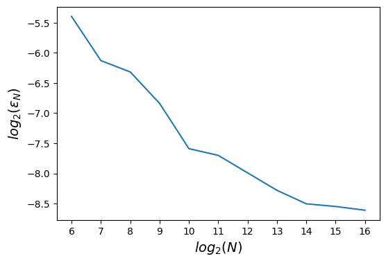
Figure 1: Log-log error (5.3) between $(X_{t})_{t\in[0,T]}$ and $(\bar{X}_{t_{m}})_{0\leq m\leq M}$ (slope = -0.35)

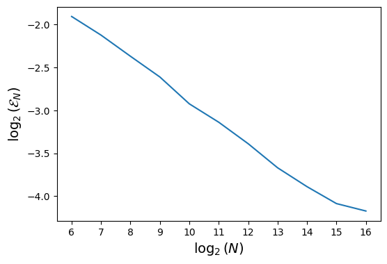
Figure 2: Log-log error (5.4) between $\hat{\mu}^{N,h,\eta}_{T}$ and $\mu_{T}$ (slope = -0.4)

5.2 Interbank market model

We consider an application from [29] where they study risk-sensitive mean field games (MFG) with common noise. It is an infinite population model where the log-reserve $(X^{i,N}_{t})_{t\in[0,T]}$ of the bank $i\in I$ at time $t\in[0,T]$ satisfies the following dynamics

$$dX^{i,N}_{t}=\Big{(}a(\bar{X}_{t}-X^{i,N}_{t})+u^{i}_{t}+b(t)\Big{)}dt+\sigma\sqrt{1-\rho^{2}}dW^{i}_{t}+\sigma\rho dW^{0}_{t},$$ (5.5)

with $\bar{X}_{t}=\lim_{N\rightarrow\infty}\frac{1}{N}\sum_{i=1}^{N}X^{i,N}_{t}$ represents the limiting market state which is following the dynamic

$$d\bar{X}_{t}=(\bar{u}_{t}+b(t))dt+\sigma\rho dW^{0}_{t},$$ (5.6)

where $\bar{u}_{t}=\lim_{N\rightarrow\infty}\frac{1}{N}\sum_{i=1}^{N}u^{i}_{t}$. The transaction $u^{i}_{t}\in\mathbb{R}$ represents the money that the bank lends to or borrows from the central bank during the market activity at each time $t$, the market shock is simulated by $W^{0}_{t}\in\mathbb{R}$ which is independent of the shock received by the bank $W^{i}_{t}\in\mathbb{R}$.

The parameter $a\in\mathbb{R}$ represents the mean reversion rate of the bank’s reserve towards the market state. The bank’s liquidity before market activity at each time $t$ is denoted by $b(t)$. The volatility of the log-reserve of the bank with respect to its own local shock (underlying uncertainty source) is given by $\sigma\rho\in\mathbb{R}$. Meanwhile, the volatility of the log-reserve with respect to the global shock that affects the market (i.e. the macroeconomic factors), is characterized by $\sigma\sqrt{1-\rho^{2}}\in\mathbb{R}$. As can be seen from above equations, an instantaneous coefficient $0\leq\rho\leq 1$ is a common multiplier factor for the shock delivered by the bank itself and by the environment.

The error analysis of this Interbank market model will proceed as follows. First, we fix $b(t)=1$ for every $t\in[0,T]$, set $a=10$ and choose $\rho\in(0,1)$ to ensure the presence of both non-zero idiosyncratic noises and common noise. Next, we compute the optimal transaction rate $(u^{i,\star}_{t})_{t\in[0,T]}$ with respect to the cost function defined by [29, Equation (134)]. It is important to note that the explicit formula for $(u^{i,\star}_{t})_{t\in[0,T]}$ depends on parameters $(\Pi_{t},\Lambda_{t},\Upsilon_{t},\Delta_{t},\Gamma_{t},\Psi_{t})_{t\in[0,T]}$, as specified in [29, Equations (139-144)] and these parameters are determined by a system of ODEs, which can be numerically solved using the Python library solve_ivp from scipy.integrate.

After computing the optimal transaction rate $(u^{i,\star}_{t})_{t\in[0,T]}$, the value of $\bar{u}^{\star}_{t}$ can be directly deduced from [29, Equation (145)] and plugged into the dynamics of $(\bar{X}_{t})_{t\in[0,T]}$ defined by (5.6). Consequently, it can be numerically solved using a standard Euler scheme for diffusion processes (see e.g. [27, Section 7.1]). On the other hand, the dynamics described by (5.5), incorporating the optimal transaction rates $(u^{i,\star}_{t})_{t\in[0,T]}$, can be computed using the particle method presented in this paper.

The simulation error is therefore evaluated as the difference between $\frac{1}{N}\sum_{i=1}^{N}X^{i,N}_{t}$, obtained from the following dynamics

$$dX^{i,N}_{t}=\left\{10\left(\frac{1}{N}\sum_{i=1}^{N}X_{t}^{i,N}-X_{t}^{i,N}\right)+u^{i,\star}_{t}+1\right\}dt+\sigma\sqrt{1-\rho^{2}}dW_{t}^{i}+\sigma\rho dW_{t}^{0},\vskip 3.0pt plus 1.0pt minus 1.0pt$$ (5.7)

and $\bar{X}_{t}$ computed by (5.6), and we perform 30 independent experiments for Monte-Carlo approximation of the expectation. More specifically, we set the time discretization number $M=100$ for both (5.6) and (5.7), and compute the simulation error using the following formula:

$$\mathcal{E}_{N}^{2}=\frac{1}{30}\sum_{j=1}^{30}\max_{1\leq m\leq M}\left\|\frac{1}{N}\sum_{i=1}^{N}X^{i,N,j}_{t_{m}}-\bar{X}^{j}_{t_{m}}\right\|^{2}.$$ (5.8)

where $j$ in the superscript of $\bar{X}^{i,N,j}_{t_{m}}$ and $\bar{X}^{j}_{t_{m}}$ denotes the index of the independent experiment, and for each fixed $j\in\{1,...,30\}$, $\bar{X}^{i,N,j}_{t_{m}},1\leq i\leq N$ is computed using the particle method (1.6) based on the dynamics in (5.7), while $\bar{X}^{j}_{t_{m}}$ is computed using a standard Euler scheme for the diffusion process (5.6). Figure 4 illustrates the log-log error of $\mathcal{E}_{N}^{2}$ defined by (5.8) and Figure 4 displays 10 simulated paths of $(X^{i,N}_{t})_{t\in[0,T]}$ under the above setting.

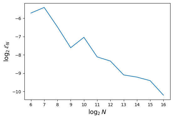
Figure 3: Log-log error of $\mathcal{E}_{N}$ defined by (5.8) (slope = -0.4)

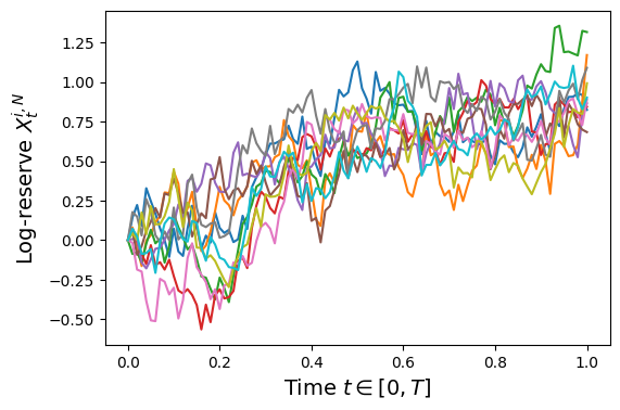
Figure 4: 10 paths of particles $(X^{i,N}_{t})_{t\in[0,T]}$

Appendix A Appendix

Proof of Lemma 2.6.

For a fixed $\omega^{0}\in\Omega^{0}$, we have

$$\mathcal{W}_{p}^{p}\big{(}\mathcal{L}^{1}(Y^{1})(\omega^{0}),\,\mathcal{L}^{1}(Y^{2})(\omega^{0})\big{)} =\mathcal{W}_{p}^{p}\big{(}\mathcal{L}(Y^{1}(\omega^{0},\cdot)),\,\mathcal{L}(Y(\omega^{0},\,\cdot))\big{)}$$

$$\leq\operatorname{\mathbb{E}}^{1}\big{[}\big{|}Y_{1}(\omega^{0},\,\cdot)-Y_{2}(\omega^{0},\,\cdot)\big{|}^{p}\big{]}$$

This inequality is true for every $\omega^{0}\in\Omega^{0}$, hence we have

$$\operatorname{\mathbb{E}}\big{[}\mathcal{W}_{p}^{p}(\mathcal{L}^{1}(Y_{1}),\mathcal{L}^{1}(Y_{2}))\big{]}\leq\operatorname{\mathbb{E}}\big{[}|Y_{1}-Y_{2}\|^{p}\big{]}$$

Then we have

$$\big{\|}\mathcal{W}_{p}(\mathcal{L}^{1}(Y_{1}),\mathcal{L}^{1}(Y_{2}))\big{\|}_{p}\leq\|Y_{1}-Y_{2}\|_{p}.\hfill\qed$$

We present the proofs of Lemma 3.2 and Lemma 3.4 required by the proof of Proposition 3.1.

Proof of Lemma 3.2.

We reason by forward induction. By Minkowski’s inequality, we have

$$\big{\|}\bar{X}_{t_{1}}\big{\|}_{p} =\big{\|}\bar{X}_{0}+h\cdot b(0,\bar{X}_{0},\bar{\mu}_{0})t_{1}+\sigma(0,\bar{X}_{0},\bar{\mu}_{0})W_{t_{1}}+\sigma^{0}(0,\bar{X}_{0},\bar{\mu}_{0})W^{0}_{t_{1}}\big{\|}_{p}$$

$$\leq\big{\|}\bar{X}_{0}\big{\|}_{p}+h\big{\|}b(0,\bar{X}_{0},\bar{\mu}_{0})\big{\|}_{p}+\sqrt{h}\big{\|}\sigma(0,\bar{X}_{0},\bar{\mu}_{0})Z_{1}\big{\|}_{p}+\sqrt{h}\big{\|}\sigma^{0}(0,\bar{X}_{0},\bar{\mu}_{0})Z^{0}_{1}\big{\|}_{p}$$

Since the solution $(X_{t})_{t\in[0,T]}$ and the continuous scheme $(\bar{X}_{t})_{t\in[0,T]}$ have the same initial condition $X_{0}$, we have, $\mathbb{P}$-almost surely

$$\bar{X}_{0}=X_{0}\in L^{p}(\Omega)\text{ and }\bar{\mu}_{0}=\mathcal{L}(X_{0}).$$

For every $0\leq m\leq M-1$, $Z_{m+1}$ and $Z^{0}_{m+1}$ are independent of $(\bar{X}_{t_{m}},\,\ldots,\bar{X}_{t_{1}},X_{0})$ and identically distributed. Moreover, since $b$, $\sigma$ and $\sigma^{0}$ have a linear growth, we have by Minkowski’s inequality

$$\big{\|}\bar{X}_{t_{1}}\big{\|}_{p} \leq\|X_{0}\|_{p}+C_{p,L,T,b,\sigma,\sigma^{0}}\big{(}1+\|X_{0}\|_{p}+\big{\|}\mathcal{W}_{p}(\mu_{0},\delta_{0})\big{\|}_{p}\big{)}\big{(}h+\sqrt{h}\|Z_{1}\|_{p}+\sqrt{h}\|Z^{0}_{1}\|_{p}\big{)}$$

$$\leq\|X_{0}\|_{p}+C_{p,L,T,b,\sigma,\sigma^{0}}\big{(}1+2\|X_{0}\|_{p}\big{)}(h+\sqrt{h}).$$

For $1\leq m\leq M-1$, we repeat the same reasoning to show that

$$\big{\|}\bar{X}_{t_{m+1}}\big{\|}_{p} \leq\|\bar{X}_{t_{m}}\|_{p}+C_{p,L,T,b,\sigma,\sigma^{0}}\big{(}1+2\|\bar{X}_{t_{m}}\|_{p}\big{)}(h+C_{p}\sqrt{h})$$

$$\leq C_{p,L,T,b,\sigma,\sigma^{0},h}^{0}\|\bar{X}_{t_{m}}\|_{p}+C_{p,L,T,b,\sigma,\sigma^{0},h}^{1}.$$

By forward induction, we have for every $0\leq m\leq M$,

$$\big{\|}\bar{X}_{t_{m}}\big{\|}_{p}\leq C\big{(}1+\|X_{0}\|_{p}\big{)},$$ (A.1)

where $C$ is a positive constant depending on the parameters $p$, $L$, $T$, $h$, $M$ and the coefficients $b$, $\sigma$ and $\sigma^{0}$. For every $t\in[0,T]$, we recall the notation $\underline{t}=t_{m}$ where $m\in\{0,\ldots,M\}$ such that $t_{m}\leq t<t_{m+1}$. By definition (1.5) of the continuous Euler scheme $(\bar{X}_{t})_{t\in[0,T]}$, it is $\mathbb{F}$-adapted and right continuous so is progressively measurable. Moreover, we have

$$\bigg{\|}\underset{0\leq t\leq T}{\sup}\big{|}\bar{X}_{t}\big{|}\bigg{\|}_{p}=\bigg{\|}\underset{0\leq t\leq T}{\sup}\Big{|}X_{0}+\int_{0}^{t}b\big{(}\underline{s},\bar{X}_{\underline{s}},\bar{\mu}_{\underline{s}}\big{)}ds+\int_{0}^{t}\sigma\big{(}\underline{s},\bar{X}_{\underline{s}},\bar{\mu}_{\underline{s}}\big{)}dW_{s}+\int_{0}^{t}\sigma^{0}\big{(}\underline{s},\bar{X}_{\underline{s}},\bar{\mu}_{\underline{s}}\big{)}dW^{0}_{s}\Big{|}\bigg{\|}_{p}$$

$$\leq\|X_{0}\|_{p}+\bigg{\|}\underset{0\leq t\leq T}{\sup}\Big{|}\int_{0}^{t}b\big{(}\underline{s},\bar{X}_{\underline{s}},\bar{\mu}_{\underline{s}}\big{)}ds\Big{|}\bigg{\|}_{p}+\bigg{\|}\underset{0\leq t\leq T}{\sup}\Big{|}\int_{0}^{t}\sigma\big{(}\underline{s},\bar{X}_{\underline{s}},\bar{\mu}_{\underline{s}}\big{)}dW_{s}\Big{|}\bigg{\|}_{p}$$

$$\hskip 45.52458pt+\bigg{\|}\underset{0\leq t\leq T}{\sup}\Big{|}\int_{0}^{t}\sigma^{0}\big{(}\underline{s},\bar{X}_{\underline{s}},\bar{\mu}_{\underline{s}}\big{)}dW^{0}_{s}\Big{|}\bigg{\|}_{p}$$

$$\leq\|X_{0}\|_{p}+\bigg{\|}\int_{0}^{T}\Big{|}b\big{(}\underline{s},\bar{X}_{\underline{s}},\bar{\mu}_{\underline{s}}\big{)}\Big{|}ds\bigg{\|}_{p}+C_{d,p}\bigg{\|}\Big{(}\int_{0}^{T}\big{|}\sigma\big{(}\underline{s},\bar{X}_{\underline{s}},\bar{\mu}_{\underline{s}}\big{)}\big{|}^{2}ds\Big{)}^{\frac{1}{2}}\bigg{\|}_{p}$$ (A.2)

$$\quad+C_{d,p}\bigg{\|}\Big{(}\int_{0}^{T}\big{|}\sigma^{0}\big{(}\underline{s},\bar{X}_{\underline{s}},\bar{\mu}_{\underline{s}}\big{)}\big{|}^{2}ds\Big{)}^{\frac{1}{2}}\bigg{\|}_{p}$$

$$\leq\|X_{0}\|_{p}+C_{L,T,b,\sigma,\sigma^{0}}\bigg{[}\int_{0}^{T}\Big{\|}\big{(}1+|\bar{X}_{\underline{s}}|+\mathcal{W}_{p}(\bar{\mu}_{\underline{s}},\delta_{0})\big{)}\Big{\|}_{p}ds+\bigg{\|}\Big{(}\int_{0}^{T}\big{|}1+|\bar{X}_{\underline{s}}|+\mathcal{W}_{p}(\bar{\mu}_{\underline{s}},\delta_{0})\big{|}^{2}ds\Big{)}^{\frac{1}{2}}\bigg{\|}_{p}\bigg{]}$$ (A.3)

where we use Minkowski’s inequality for the first inequality, the second inequality follows from Lemma 2.4 and the linear growth of the coefficients. By applying Young’s inequality on (A.3), we can infer that

$$\bigg{\|}\underset{0\leq t\leq T}{\sup}\big{|}\bar{X}_{t}\big{|}\bigg{\|}_{p}$$

$$\leq\|X_{0}\|_{p}+C_{L,T,d,p,b,\sigma,\sigma^{0}}\bigg{[}\int_{0}^{T}\big{(}1+2\|\bar{X}_{\underline{s}}\|_{p}\big{)}ds+\sqrt{T}+\bigg{(}\int_{0}^{T}\|\bar{X}_{\underline{s}}\|_{p}^{2}ds\bigg{)}^{\frac{1}{2}}+\bigg{(}\int_{0}^{T}\mathcal{W}_{p}^{2}(\bar{\mu}_{\underline{s}},\delta_{0})ds\bigg{)}^{\frac{1}{2}}\bigg{]}$$

$$\leq\|X_{0}\|_{p}+C_{L,T,d,p,b,\sigma,\sigma^{0}}\bigg{[}\int_{0}^{T}\big{(}1+2\|\bar{X}_{\underline{s}}\|_{p}\big{)}ds+\bigg{(}\int_{0}^{T}\|\bar{X}_{\underline{s}}\|_{p}^{2}ds\bigg{)}^{\frac{1}{2}}\bigg{]},$$

from Lemma 2.6. Then we deduce the following inequality to which we apply Lemma 2.5

$$\bigg{\|}\underset{0\leq t\leq T}{\sup}\big{|}\bar{X}_{t}\big{|}\bigg{\|}_{p}\leq\|X_{0}\|_{p}+C_{L,T,d,p,b,\sigma,\sigma^{0}}\bigg{[}\int_{0}^{T}\Big{\|}\sup_{0\leq u\leq s}|\bar{X}^{M}_{u}|\Big{\|}_{p}ds+\bigg{(}\int_{0}^{T}\Big{\|}\sup_{0\leq u\leq s}|\bar{X}^{M}_{u}|\Big{\|}_{p}^{2}ds\bigg{)}^{\frac{1}{2}}\bigg{]}.$$ (A.4)

Since $\bar{X}^{M}\in\mathbb{L}^{p}$, the application $t\mapsto\Big{\|}\sup_{0\leq u\leq t}\bar{X}^{M}_{u}\Big{\|}_{p}$ is continuous, non-negative and non-decreasing on $[0,T]$, the final estimate follows from Lemma 2.5

$$\bigg{\|}\underset{0\leq t\leq T}{\sup}\big{|}\bar{X}_{t}\big{|}\bigg{\|}_{p}\leq\tilde{C}\big{(}1+\|X_{0}\|_{p}\big{)},$$

where $\tilde{C}$ is a positive constant depending on $p$, $L$, $T$, $h$, $M$ and the coefficients $b$, $\sigma$ and $\sigma^{0}$. Hence $\bar{X}\in\mathbb{L}^{p}([0,T]\times\Omega)$. ∎

Proof of Lemma 3.3.

The first step of the proof is inspired by the proof of [9, Proposition 2.9]. The first additional step is to combine the results of the Lemmas 2.1 and 3.2, that is $(\bar{X}_{t})_{t\in[0,T]}\in\mathbb{L}^{p}([0,T]\times\Omega)$ and $\mathcal{L}^{1}(\bar{X}_{t})_{t\in[0,T]}$ has continuous paths in $\mathcal{P}_{p}(\operatorname{\mathbb{R}}^{d})$ and is $\mathbb{F}^{0}$-adapted. The second one follows directly from the construction of the Euler scheme $(\bar{X}_{t})_{t\in[0,T]}$. There exists a unique process that satisfies Equation (1.5) for the Brownian motions $(W_{t})_{t\in[0,T]}$ and $(W^{0}_{t})_{t\in[0,T]}$. The second step is a consequence of Lemma 2.1 and Lemma 3.2. ∎

Proof of Lemma 3.4.

Set $(\mu_{t})_{t\in[0,T]}=\big{(}\mathcal{L}^{1}(X_{t})\big{)}_{t\in[0,T]}$. Fix $s,t\in[0,T]$ such that $s\leq t$. Since $(X_{t})_{t\in[0,T]}$ solves the McKean-Vlasov equation with common noise (1.1), we have

$$\big{\|}X_{t}-X_{s}\big{\|}_{p}=\bigg{\|}\int_{s}^{t}b(u,X_{u},\mu_{u})du+\int_{s}^{t}\sigma(u,X_{u},\mu_{u})dW_{u}+\int_{s}^{t}\sigma^{0}(u,X_{u},\mu_{u})dW^{0}_{u}\bigg{\|}_{p}$$

$$\leq\bigg{\|}\int_{s}^{t}b(u,X_{u},\mu_{u})du\bigg{\|}_{p}+\bigg{\|}\int_{s}^{t}\sigma(u,X_{u},\mu_{u})dW_{u}\bigg{\|}_{p}+\bigg{\|}\int_{s}^{t}\sigma^{0}(u,X_{u},\mu_{u})dW^{0}_{u}\bigg{\|}_{p}$$

$$\leq\int_{s}^{t}\big{\|}b(u,X_{u},\mu_{u})\big{\|}_{p}du+C_{d,p}\bigg{\|}\Big{(}\int_{s}^{t}\sigma(u,X_{u},\mu_{u})^{2}du\Big{)}^{\frac{1}{2}}\bigg{\|}_{p}+C_{d,p}\bigg{\|}\Big{(}\int_{s}^{t}\sigma^{0}(u,X_{u},\mu_{u})^{2}du\Big{)}^{\frac{1}{2}}\bigg{\|}_{p}$$

$$=\int_{s}^{t}\big{\|}b(u,X_{u},\mu_{u})\big{\|}_{p}du+C_{d,p}\bigg{\|}\int_{s}^{t}\sigma(u,X_{u},\mu_{u})^{2}du\bigg{\|}_{\frac{p}{2}}^{\frac{1}{2}}+C_{d,p}\bigg{\|}\int_{s}^{t}\sigma^{0}(u,X_{u},\mu_{u})^{2}du\bigg{\|}_{\frac{p}{2}}^{\frac{1}{2}}$$

$$\leq\int_{s}^{t}\big{\|}b(u,X_{u},\mu_{u})\big{\|}_{p}du+C_{d,p}\bigg{(}\int_{s}^{t}\big{\|}\sigma(u,X_{u},\mu_{u})^{2}\big{\|}_{\frac{p}{2}}du\bigg{)}^{\frac{1}{2}}+C_{d,p}\bigg{(}\int_{s}^{t}\big{\|}\sigma^{0}(u,X_{u},\mu_{u})^{2}\big{\|}_{\frac{p}{2}}du\bigg{)}^{\frac{1}{2}}$$

$$=\int_{s}^{t}\big{\|}b(u,X_{u},\mu_{u})\big{\|}_{p}du+C_{d,p}\bigg{(}\int_{s}^{t}\big{\|}\sigma(u,X_{u},\mu_{u})\big{\|}_{p}^{2}du\bigg{)}^{\frac{1}{2}}+C_{d,p}\bigg{(}\int_{s}^{t}\big{\|}\sigma^{0}(u,X_{u},\mu_{u})\big{\|}_{p}^{2}du\bigg{)}^{\frac{1}{2}}.$$

where we used the Minkowski’s inequality at the first inequality, the second one follows from the general Minkowski’s (Lemma 2.3) and Burkölder-Davis-Gundy inequalities (Lemma 2.4) and the general Minkowski’s inequality provides the last one. We use the linear growth of the coefficients and Minkowski’s and Young’s inequalities to get that

$$\big{\|}X_{t}-X_{s}\big{\|}_{p}\leq C_{L,T,b,\sigma,\sigma^{0}}\bigg{(}\int_{s}^{t}\big{\|}1+|X_{u}|+\mathcal{W}_{p}(\mu_{u},\delta_{0})\big{\|}_{p}du+2\bigg{[}\int_{s}^{t}\big{\|}1+|X_{u}|+\mathcal{W}_{p}(\mu_{u},\delta_{0})\big{\|}_{p}^{2}du\bigg{]}^{\frac{1}{2}}\bigg{)}$$

$$\leq C_{L,T,b,\sigma,\sigma^{0}}\bigg{(}\int_{s}^{t}\big{(}1+\big{\|}X_{u}\big{\|}_{p}+\big{\|}\mathcal{W}_{p}(\mu_{u},\delta_{0})\big{\|}_{p}\big{)}du+2\bigg{[}\int_{s}^{t}\big{(}1+\big{\|}X_{u}\big{\|}_{p}+\big{\|}\mathcal{W}_{p}(\mu_{u},\delta_{0})\big{\|}_{p}\big{)}^{2}du\bigg{]}^{\frac{1}{2}}\bigg{)}$$

$$\leq C_{L,T,b,\sigma,\sigma^{0}}\bigg{(}\int_{s}^{t}\big{(}1+\big{\|}X_{u}\big{\|}_{p}\big{)}du+\bigg{[}\int_{s}^{t}\big{(}1+\big{\|}X_{u}\big{\|}_{p}\big{)}^{2}du\bigg{]}^{\frac{1}{2}}\bigg{)}$$

$$\leq C_{L,T,b,\sigma,\sigma^{0}}\bigg{(}\int_{s}^{t}\big{(}1+\big{\|}X_{u}\big{\|}_{p}\big{)}du+\bigg{[}\int_{s}^{t}\big{(}1+\big{\|}X_{u}\big{\|}_{p}^{2}\big{)}du\bigg{]}^{\frac{1}{2}}\bigg{)}$$

$$\leq C_{L,T,b,\sigma,\sigma^{0}}\bigg{[}\bigg{(}1+\bigg{\|}\underset{0\leq t\leq T}{\sup}|X_{t}|\bigg{\|}_{p}\bigg{)}(t-s)+\bigg{(}1+\bigg{\|}\underset{0\leq t\leq T}{\sup}|X_{t}|\bigg{\|}_{p}^{2}\bigg{)}^{\frac{1}{2}}\sqrt{t-s}\bigg{]}$$

$$\leq\kappa\,\sqrt{t-s}\quad\text{(by Inequality \eqref{eq : estimate MKV solution})}.$$

where $\kappa$ is a positive constant depending on $p$, $L$, $T$, $b$, $\sigma$, $\sigma^{0}$, and $\|X_{0}\|_{p}$. Then we have

$$\big{\|}X_{t}-X_{s}\big{\|}_{p}\leq\kappa\sqrt{t-s}.\hfill\qed$$

Proof of Lemma 4.1.

The particles $(\bar{Y}^{i}_{t})_{1\leq i\leq N}$ are copies of the continuous of the continuous extension $\bar{X}$ of the Euler scheme (1.5). From (4.1), for every $1\leq i\leq N$, there exists a measurable function $\Psi^{i}$ on $\operatorname{\mathbb{R}}^{d}\times\mathcal{C}([0,T],\operatorname{\mathbb{R}}^{q})\times\mathcal{C}([0,T],\operatorname{\mathbb{R}}^{q})$ such that:

$$\bar{Y}^{i}=\Psi^{i}\Big{(}X_{0}^{i},(W^{i}_{t})_{0\leq t\leq T},(W^{0}_{t})_{0\leq t\leq T}\Big{)}.$$

As the idiosyncratic noises and the initial random variables $(W^{i},X_{0}^{i})_{1\leq i\leq N}$ are i.i.d. by definition, the particles $(\bar{Y}^{i})_{1\leq i\leq N}$ are identically distributed and independent conditionally to $W^{0}$. ∎

References

- [1] S. Ahuja “Wellposedness of mean field games with common noise under a weak monotonicity condition” In SIAM J. Control Optim. 54.1, 2016, pp. 30–48 DOI: 10.1137/140974730
- [2] F. Antonelli and A. Kohatsu-Higa “Rate of convergence of a particle method to the solution of the McKean-Vlasov equation” In Ann. Appl. Probab. 12.2, 2002, pp. 423–476 DOI: 10.1214/aoap/1026915611
- [3] J. Baladron, D. Fasoli, O. Faugeras and J. Touboul “Mean-field description and propagation of chaos in networks of Hodgkin-Huxley and FitzHugh-Nagumo neurons” In J. Math. Neurosci. 2, 2012, pp. Art. 10\bibrangessep50 DOI: 10.1186/2190-8567-2-10
- [4] S. Biswas et al. “An explicit Milstein-type scheme for interacting particle systems and McKean-Vlasov SDEs with common noise and non-differentiable drift coefficients” In Ann. Appl. Probab. 34.2, 2024, pp. 2326–2363 DOI: 10.1214/23-aap2024
- [5] M. Bossy, J.-F. Jabir and K. Martínez Rodríguez “Instantaneous turbulent kinetic energy modelling based on Lagrangian stochastic approach in CFD and application to wind energy” In J. Comput. Phys. 464, 2022, pp. Paper No. 110929\bibrangessep29 DOI: 10.1016/j.jcp.2021.110929
- [6] M. Bossy and D. Talay “A stochastic particle method for the McKean-Vlasov and the Burgers equation” In Math. Comp. 66.217, 1997, pp. 157–192 DOI: 10.1090/S0025-5718-97-00776-X
- [7] P. Cardaliaguet and C.-A. Lehalle “Mean field game of controls and an application to trade crowding” In Math. Financ. Econ. 12.3, 2018, pp. 335–363 DOI: 10.1007/s11579-017-0206-z
- [8] R. Carmona and F. Delarue “Probabilistic theory of mean field games with applications. I” Mean field FBSDEs, control, and games Springer, Cham, 2018, pp. xxv+713
- [9] R. Carmona and F. Delarue “Probabilistic theory of mean field games with applications. II” Mean field games with common noise and master equations Springer, Cham, 2018, pp. xxiv+697
- [10] R. Carmona, F. Delarue and D. Lacker “Errata: Mean field games with common noise” In Ann. Probab. 48.5, 2020, pp. 2644–2646 DOI: 10.1214/20-AOP1432
- [11] J.-F. Chassagneux and G. Pagès “Computing the invariant distribution of McKean-Vlasov SDEs by ergodic simulation” In arXiv preprint arXiv:2406.13370, 2024
- [12] X. Chen and G. Reis “A flexible split-step scheme for solving McKean-Vlasov stochastic differential equations” In Appl. Math. Comput. 427, 2022, pp. Paper No. 127180\bibrangessep23 DOI: 10.1016/j.amc.2022.127180
- [13] F. Delarue “Restoring uniqueness to mean-field games by randomizing the equilibria” In Stoch. Partial Differ. Equ. Anal. Comput. 7.4, 2019, pp. 598–678 DOI: 10.1007/s40072-019-00135-9
- [14] F. Delarue and R. Foguen Tchuendom “Selection of equilibria in a linear quadratic mean-field game” In Stochastic Process. Appl. 130.2, 2020, pp. 1000–1040 DOI: 10.1016/j.spa.2019.04.005
- [15] N. Fournier and A. Guillin “On the rate of convergence in Wasserstein distance of the empirical measure” In Probab. Theory Related Fields 162.3-4, 2015, pp. 707–738 DOI: 10.1007/s00440-014-0583-7
- [16] P. Graber “Linear quadratic mean field type control and mean field games with common noise, with application to production of an exhaustible resource” In Appl. Math. Optim. 74.3, 2016, pp. 459–486 DOI: 10.1007/s00245-016-9385-x
- [17] M. Hoffmann and Y. Liu “A statistical approach for simulating the density solution of a McKean-Vlasov equation” working paper or preprint, 2023 URL: https://hal.science/hal-04096108
- [18] M. Kac “Foundations of kinetic theory” In Proceedings of The third Berkeley symposium on mathematical statistics and probability 3.600, 1956, pp. 171–197
- [19] D. Lacker “Hierarchies, entropy, and quantitative propagation of chaos for mean field diffusions” In Probab. Math. Phys. 4.2, 2023, pp. 377–432 DOI: 10.2140/pmp.2023.4.377
- [20] D. Lacker “Mean Field Games and interacting particle systems”
- [21] D. Lacker “On a strong form of propagation of chaos for McKean-Vlasov equations” In Electron. Commun. Probab. 23, 2018, pp. Paper No. 45\bibrangessep11 DOI: 10.1214/18-ECP150
- [22] D. Lacker and K. Webster “Translation invariant mean field games with common noise” In Electron. Commun. Probab. 20, 2015, pp. no. 42\bibrangessep13 DOI: 10.1214/ECP.v20-3822
- [23] J.-M. Lasry and P.-L. Lions “Mean-field games with a major player” In Comptes Rendus Mathematique 356.8, 2018, pp. 886–890 DOI: https://doi.org/10.1016/j.crma.2018.06.001
- [24] Y. Liu “Particle method and quantization-based schemes for the simulation of the McKean-Vlasov equation” In ESAIM Math. Model. Numer. Anal. 58.2, 2024, pp. 571–612 DOI: 10.1051/m2an/2024007
- [25] N. Martzel and C. Aslangul “Mean-field treatment of the many-body Fokker-Planck equation” In J. Phys. A 34.50, 2001, pp. 11225–11240 DOI: 10.1088/0305-4470/34/50/305
- [26] H.. McKean “A class of Markov processes associated with nonlinear parabolic equations” In Proc. Nat. Acad. Sci. U.S.A. 56, 1966, pp. 1907–1911 DOI: 10.1073/pnas.56.6.1907
- [27] G. Pagès “Numerical Probaility” Springer, 2018
- [28] G. Reis, S. Engelhardt and G. Smith “Simulation of McKean-Vlasov SDEs with super-linear growth” In IMA J. Numer. Anal. 42.1, 2022, pp. 874–922 DOI: 10.1093/imanum/draa099
- [29] X. Ren and D. Firoozi “Risk-Sensitive Mean Field Games with Common Noise: A Theoretical Study with Applications to Interbank Markets” In arXiv preprint arXiv:2403.03915, 2024
- [30] A.-S. Sznitman “Topics in propagation of chaos” In École d’Été de Probabilités de Saint-Flour XIX—1989 1464 Springer, Berlin, 1991, pp. 165–251 DOI: 10.1007/BFb0085169