Generalizing causal effect estimates to larger populations while accounting for (uncertainty in) effect modifiers using a scaled Bayesian bootstrap with application to estimating the effect of family planning on employment in Nigeria

Abstract

Strategies are needed to generalize causal effects from a sample that may differ systematically from the population of interest. In a motivating case study, interest lies in the causal effect of family planning on empowerment-related outcomes among urban Nigerian women, while estimates of this effect and its variation by covariates are available only from a sample of women in six Nigerian cities. Data on covariates in target populations are available from a complex sampling design survey. Our approach, analogous to the plug-in g-formula, takes the expectation of conditional average treatment effects from the source study over the covariate distribution in the target population. This method leverages generalizability literature from randomized trials, applied to a source study using principal stratification for identification. The approach uses a scaled Bayesian bootstrap to account for the complex sampling design. We also introduce checks for sensitivity to plausible departures of assumptions. In our case study, the average effect in the target population is higher than in the source sample based on point estimates and sensitivity analysis shows that a strong omitted effect modifier must be present in at least 40% of the target population for the 95% credible interval to include the null effect.

, and

1 Introduction

In this paper, we consider how to generalize causal effect estimates from small source populations to larger target populations while accounting for (uncertainty in) effect modifiers. This analysis is motivated by interest in estimating the effect of family planning (e.g., modern contraceptive use) on empowerment related outcomes (e.g., employment) among a broad population of Nigerian women (i.e., woman of reproductive age living in urban areas who have not used modern contraceptives but wish to avoid or delay pregnancy). An estimate of the effect of modern contraceptive adoption on employment, and how this effect varies as a function of baseline characteristics (i.e., effect modifiers), is available from a sample of women from 6 cities in Nigeria who were not using modern contraceptives at baseline and whose subsequent uptake was affected by the early rollout of a family planning (FP) program (Garraza, Speizer and Alkema (2024) [GSA24 onwards]). However, there may be systematic differences between the women from the sample (referred to as the source) and the population of interest (referred to as the target), and those differences may modify the effect of adopting modern contraception on women’s employment. The question of interest is how to generalize from the source to the target population while accounting for differences in the distribution of effect modifiers.

There is an increasing body of causal inference literature on generalizability (also discussed as transportability, recoverability, and external validity). Recent reviews were undertaken by Degtiar and Rose (2023) and Colnet et al. (2023). The topic is also discussed in Li, Ding and Mealli (2022) from a Bayesian perspective. The approach that we follow in this paper is to estimate the population average treatment effect (PATE) for the target population from conditional average treatment effects (CATEs) obtained from a source study. While the approach is not new, most of the literature has focused on generalizing from randomized trials rather than from observational studies using principal stratification or instrumental variables for identification of the CATEs.

When estimating a PATE, an open challenge is how to account for additional uncertainty in the distribution of effect modifiers in the target population when effect modifier data comes from a survey with a complex sample design. This challenge applies to our motivating example, as information from the target population is available only from household surveys that follow a complex sampling design (NPC and ICF, 2019). Bayesian bootstrap (BB) approaches have been proposed in the context where effect modifier data are available from a random sample from the target population (see e.g., Hill (2011); Oganisian, Mitra and Roy (2022); Taddy et al. (2016); Wang et al. (2015); Xu, Daniels and Winterstein (2018)). However, these existing approaches have not considered the setting where covariate data from the target population were obtained through a survey with a complex sampling design. We consider innovations in survey sampling literature to handle complex survey samples in the context of our causal inference generalization problem.

Our paper is organized as follows. The next section introduces the motivating example in greater detail, followed by a section that reviews the relevant literature on generalization and working with complex survey data. The methods section introduces the approach to estimate PATEs using CATEs from a source population and complex survey data from the target population. This section identifies assumptions needed for the generalization procedure to be valid and provides approaches to gauge the sensitivity of the results to departures from those assumptions. We check the approach through simulation studies and apply it to estimate the effect of modern contraceptive use on employment among broad populations of Nigerian women. We end with a discussion of our approach and its limitations.

2 Background and motivation

A prior study (GSA24) estimated the effect of adoption of modern contraception on employment four years after baseline among women who were impacted by an FP program. The program was initially introduced in 2010/2011 in four cities (Abuja, Ibadan, Ilorin, and Kaduna). After two years of implementation, the program was extended to two additional cities: Benin City and Zaria. Longitudinal data on a sample of 6,808 who had never used modern contraception was collected prior to the start of the FP interventions (baseline) and four years after (endline). To ensure internal validity, estimates of the effect of adoption of contraception on employment were based on a very selective subsample, namely women affected by the early rollout of the program (termed ”compliers”). The estimation included not only the overall effect in that subsample, but also how the effect varied as a function of baseline characteristics (i.e., the conditional average treatment effect (CATE)) thanks to the use of a flexible approach based on Bayesian Additive Regression Trees (BART).

Figure 1, taken from GSA24, shows the estimated effect for women in eight mutually exclusive subgroups, with subgroups based on covariate combinations that were identified as the main effect modifiers (how the estimation was carried out and these groups identified is described in source study). The difference between the largest effect (among women who worked during the year before baseline, were married at baseline, and were in the lower and lowest wealth groups) and the smallest one (among women who had not worked during the year before baseline, were never married at baseline, and were in the medium to highest wealth groups) is significant in the sense that the probability that the difference between the two effects is greater than zero exceeds 99.8% (GSA24).

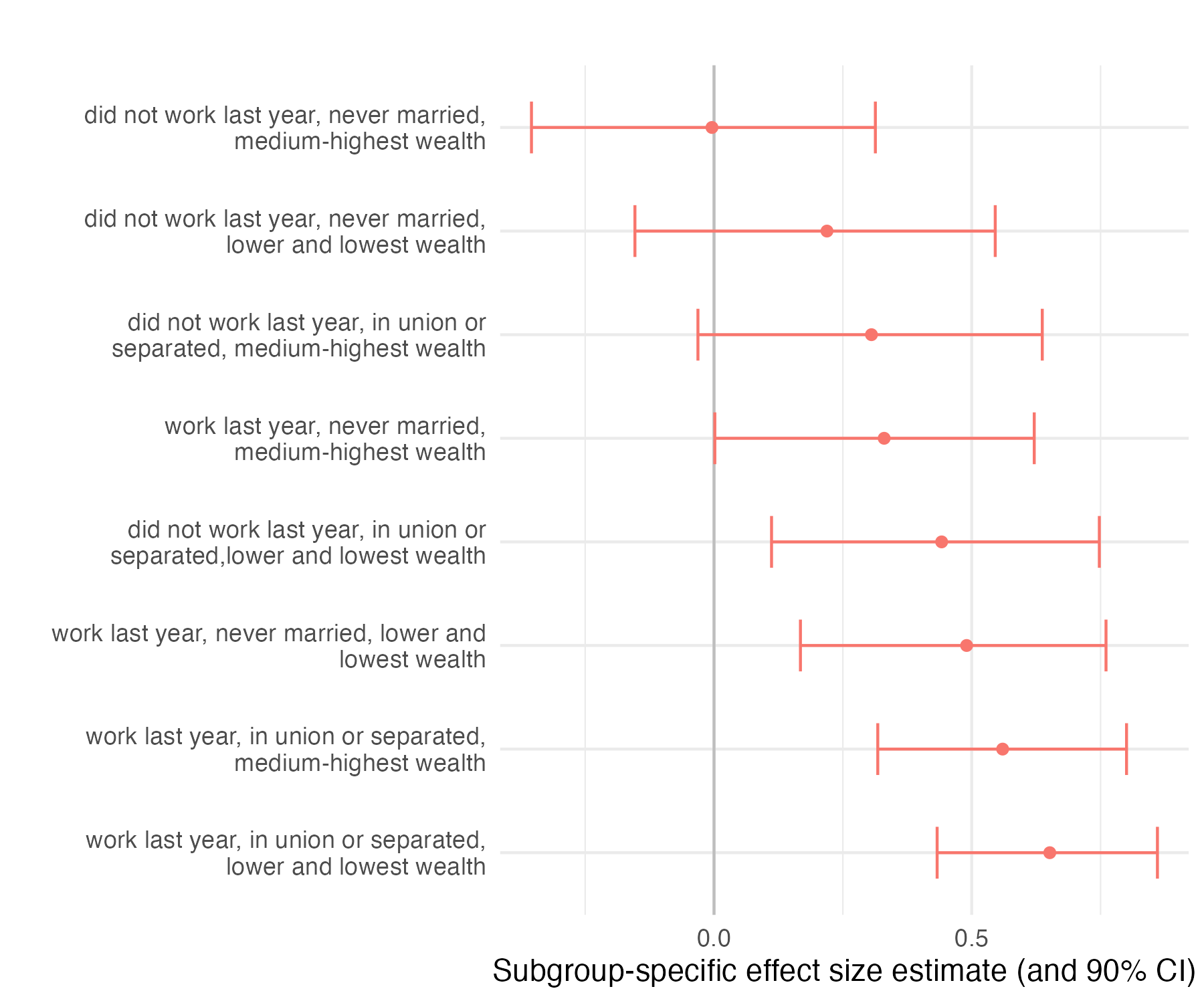
Figure 1: Effect of contraceptive use on employment as a function of selected baseline combination of covariates in the source study. Segments are mutually exclusive. They were identified with a regression tree to select those combinations of baseline covariates that best predicted differences in effect sizes (figure taken from GSA24).

We are interested in generalizing the results from the selective sample in GSA24 (the source study) to a larger population of interest, such as all women in urban areas in Nigeria who had not used contraception previously and wish to avoid or delay pregnancy. Specifically, we wonder what effect on employment could be expected four years from baseline if all women from the population of interest were to adopt modern contraceptives within the four years after baseline. Other populations of interest may include all women in Nigeria. For this target population, we note that the source study did not include women from rural areas, hence there may be issues related to unobserved differences between these populations. We return to this issue at a later point. We also note that we do not address how the adoption of contraceptives occurs in the population of interest, if at all. Instead, we focus on the effect such adoption would have.

Covariate data on the target population is available from Nigeria’s Demographic and Health Survey (DHS, Corsi et al. (2012)). The DHS is a standardized household survey conducted periodically on over 90 countries since 1984 with the support of the United States Agency for International Development (USAID). DHS is widely regarded as a reference source for population descriptive information in family planning and other health topics in low- and middle-income countries. For that reason, most variables used in GSA24 are also measured in the DHS and were operationalized in the same way. Hence the DHS contains information on the distribution in the target population of the covariates included in the source data.

We use data from the Nigeria DHS carried out in 2018 (NPC and ICF (2019)), which, following the DHS general practices, is based on a complex sampling design. Specifically, the NDHS18 is based on a stratified two-stage probabilistic sample of approximately 42,000 households. The strata are defined by dividing each of the 36 states into rural and urban regions. Independently for each stratum, a sample of compact geographic units referred as primary sample units (PSUs) is selected with probability proportional to size (PPS), were the best available information on the number of households is used as measure of size. After listing all household across the 1,400 sampled PSUs, a systematic random sample of 30 households per PSU is taken. DHS attempts to interview all women aged 15 to 49 residing in the selected households. The publicly released dataset includes sample weights computed to reflect the inclusion and response probabilities. In the case of DHS, nonresponse adjustment varies only by strata and there is poststratification or calibration.

Figure 2 shows the proportion of women in each of the eight subgroups introduced in Figure 1 among compliers in the source study and among three possible target populations. The three target populations are (1) all women residing in urban areas in the 5 states represented in the source study, (2) all women residing in urban areas, and (3) all women in Nigeria. For the target populations, the estimates of the proportion of women in each segment are based on the NDHS18 (the DHS questions used to identified these populations are listed in Appendix I). It is apparent that the distribution of effect modifiers is not the same across the four populations. In particular, groups were the effect was larger are more prevalent in the target populations than they are among compilers in the source study, while the opposite is true for groups with smaller effects.

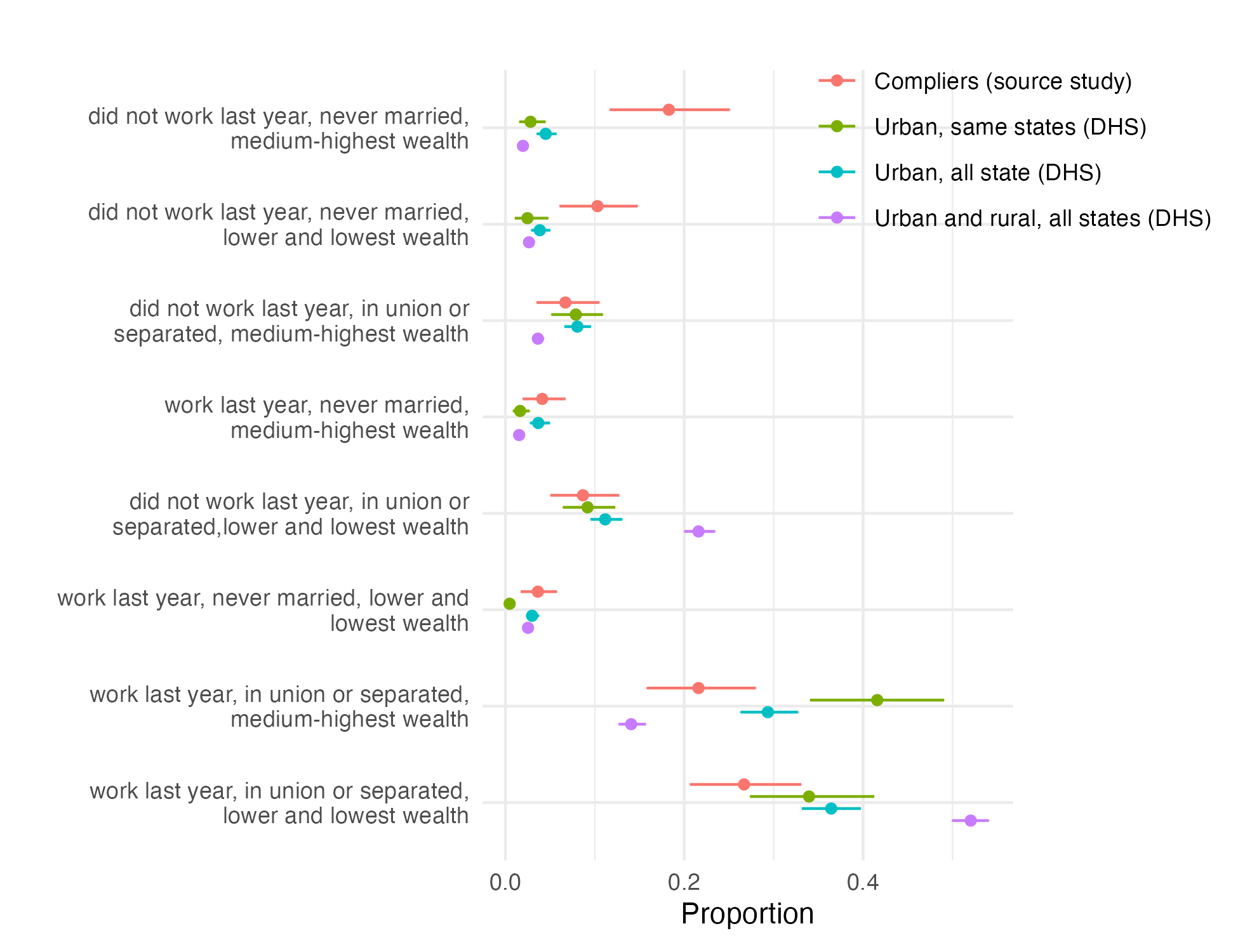
Figure 2: Proportion of women in different effect modifier subgroups for four populations: (1) compliers in the source study, and, based on the 2018 DHS information, (2) all women residing in urban areas in the 5 states represented in the source study, (3) all women residing in urban areas, and (4) all women in Nigeria. Lines represent 95% credible intervals. (Additional baseline characteristics are included in Appendix I.)

Given differences in effect modifier distributions between source and target populations, we might expect differences in average marginal effect of contraceptive use on women’s employment between source and target populations. The remainder of the paper consider approaches to produce such estimates.

3 Related literature

Our method leverages recent advances in generalizability from randomized trials to generalize findings from a source study that uses principal stratification for identification. Specifically, we estimate the population average treatment effect (PATE) for the target population from conditional average treatment effects (CATEs) obtained from a source study.

The large and growing body of literature on generalizing or transporting results from randomized trials considers the issue that participants are rarely a probabilistic sample from the population of interest. Recent reviews include Degtiar and Rose (2023) and Colnet et al. (2023). The topic is also discussed in Li, Ding and Mealli (2022) from a Bayesian perspective. Most of the this work has focused on addressing observed discrepancies in the distribution of potential effect modifiers between the source study and target population, leveraging information on the target population from additional studies (e.g., cole_generalizing_2010). Our approach is aligned with this literature; we combine covariate information from the target population with CATEs from the source study.

Prior literature has considered how to generalize from studies that use principal stratification or instrumental variables to identify the causal effect of interest, including trials with imperfect compliance or randomized encouragement designs (Angrist and Fernandez-Val (2010); Aronow and Carnegie (2013); Hernán and Robins (2006); Rudolph and Laan (2017); Wang and Tchetgen Tchetgen (2018)). Collectively, this work has clarified the assumptions required for generalization from such studies. Further, both Angrist and Fernandez-Val (2010) and Rudolph and Laan (2017) consider ways to address observed covariates shifts across populations. Our setting and approach are somewhat different from existing work, however, in two ways. Firstly, we only assume access to covariate information from the target population. In particular, we do not assume any information on the instrument in the population. Secondly, we leverage flexibly estimated CATEs from the source study, i.e., CATEs that were estimated from combining principle stratification with Bayesian Additive Regression Trees (BART).

We use a Bayesian bootstrap to combine CATEs with external information on the distribution of covariates in the target population. An early proposal to combine CATEs with covariate information from the target population is discussed in Hill, (2011, Appendix A). Hill proposed to either ignore the additional estimation uncertainty in the covariate density (if the external sample was very large) or use a frequentist bootstrap to incorporate it. Our approach builds off several recent applications that have used the Bayesian counterpart, i.e., the Bayesian bootstrap (BB), to incorporate the uncertainty introduced by the estimation of the covariate distribution in the target population while avoiding the need to specify a full parametric model (e.g., Oganisian, Mitra and Roy (2022); Taddy et al. (2016); Wang et al. (2015); Xu, Daniels and Winterstein (2018)).

We use a modified version of the Bayesian bootstrap to account for the complex sampling design associated with the covariate data. In its original formulation, the BB as introduced by Rubin (1981) (see also Chamberlain and Imbens (2003)) assumes the data is independent and identically distributed (i.i.d.) generated. This approach is not appropriate in our application, due to the complex sampling design that was used to collect the covariate data on the target population. How to address complex sampling design in Bayesian estimation has been subject to long-standing debates (see Little (2014) for an interesting account). Some extensions of the BB to handle complex samples have been proposed, including sampling from finite population (Lo (1988)), unequal probability sampling (Cohen (1997); Rao and Wu (2010); Zangeneh and Little (2015)), and the combination of stratification and clustering (Aitkin (2008); Dong, Elliott and Raghunathan (2014); Makela, Si and Gelman (2018)). To the best of our knowledge, these innovations have not yet been applied to causal inference.

4 Methods

4.1 Set up and notation

Let $i=1,\ldots,\ n,$ index the unit in the source study and $i=n+1,\ldots,\ n+m$ the unit in the population of interest. In our application, the units are women. Denote by $\mathcal{S}$ (for source) and $\mathcal{T}$ (for target) the two sets of indices. Let $T_{i}$ indicate if a unit was part of the source study or is part of the target population, with $T_{i}=1$ if $i\in\mathcal{T}$ and zero otherwise. For each woman in the source study sample as well as for a large sample of women from the target population, we observe a set covariate characteristic, $X_{i}$, including baseline values of the outcomes of interest.

The source study generated estimates of how the causal effect of a binary variable, $W_{i}$, on an outcome of interest, $Y_{i}$, varies as a function of baseline covariates among certain subsample of units, i.e.,

$${CATE}_{c}(x)\equiv\mathbb{E}\left(Y_{i}^{*}(1)-Y_{i}^{*}(0)\middle|X_{i}=x,\ C_{i}^{*}=1\right),$$ (1)

where $Y_{i}^{*}(w)$, for w = 0, 1, denotes the potential outcome for each unit if the variable W were to take the value w (Rubin, 1974), $C_{i}^{*}$ indicates membership to the subsample from which causal estimates were obtained, with $C_{i}^{*}=1$ if the unit is in that subsample and $C_{i}^{*}=0$ if not.

While for a RCT with perfect compliance the value of $C_{i}^{*}$ is known, i.e., $C_{i}^{*}=\left(1-T_{i}\right)$, for a source study that used principal stratification, $C_{i}^{*}$ is a latent variable that refers to those units that complied with the treatment assignment, referred to as compliers. In either case, the subpopulation with $C_{i}^{*}=1$ (members of a latent stratum or participants in an RCT) may not correspond to the population of interest, and additional assumption are required to generalize or transport the results to the later one. In our application, the compliers are those women who started using modern contraceptive methods because a FP program was rolled out early, as well as those women who did not start using modern contraceptive methods but would have, if contrary to fact they had also been exposed to the early roll out. We note that, regardless of the latent nature of $C_{i}^{*}$, it is still possible to estimate any aspect of the covariate distribution among compliers, which allows to examine covariate overlap with the target population, for example.

4.2 Estimand

We are interested in the average effect of contraceptive use on employment in the target population. The population average treatment effect (PATE) for this population is defined as

$$PATE\equiv\mathbb{E}\left(Y_{i}^{*}(1)-Y_{i}^{*}(0)\mid T_{i}=1\right),$$ (2)

where the expectation is taken over the entire target population of interest. For the application, for example, the population of interest are women residing in urban Nigeria who have not used modern contraception (i.e., the inclusion criteria for GSA24) and wish to avoid or delay pregnancy (i.e., may benefit from adopting modern contraceptives).

An equivalent expression for the PATE is,

$$PATE=\mathbb{E}_{X\mid T=1}\left(CATE(X_{i})\right)=\int CATE(x)dP_{X\mid T=1}(x),$$ (3)

where $CATE(x)\mathbb{\equiv\ E}\left(Y_{i}^{*}(1)-Y_{i}^{*}(0)\middle|X_{i}=x\ \right)$ is the conditional average treatment effect and $P_{X|T=1}(x)$ the distribution of covariates in the population of interest.

4.3 Identifying assumptions

To be able to generalize the results from the source study the following two assumptions are sufficient.

Assumption 1.

(conditional transportability)

$$\mathbb{E}\left(Y_{i}^{*}(1)-Y_{i}^{*}(0)\middle|X_{i},\ C_{i}^{*}=1\right)\mathbb{=E}\left(Y_{i}^{*}(1)-Y_{i}^{*}(0)\middle|X_{i}\right),$$

where $C_{i}^{*}=1$ indicates membership to the latent stratum from which causal estimates were obtained, i.e., the compliers. This assumption is discussed in by Angrist and Fernandez-Val (2010), under the rubric ”conditional effect ignorability”, and Aronow and Carnegie (2013), who termed it ”latent ignorability of compliance with respect to treatment effect heterogeneity”. We note that the assumption is formally similar to one used to generalize or transport results from an RCT with perfect compliance, with $C_{i}^{*}$ set to $\left(1-T_{i}\right)$ (Colnet et al. (2022, 2023)).

As discussed by Wang and Tchetgen Tchetgen (2018), one of two conditions suffice for assumption 1 to hold. To describe these conditions, it is convenient to introduce additional notation. Let $U_{i}$ be an unobserved factor confounding the relation between W and Y, such that W is independent of the potential outcomes, only after conditioning on U in addition to the observed covariates, i.e., $W_{i}\bot Y_{i}(w)|X_{i},U_{i},$ for $w=0,\ 1$. The possibility of $U_{i}$ motivated the use of principal stratification for identification in the source study (or the use of RCT’s, when randomization of $W_{i}$ is feasible). As point out by Wang and Tchetgen Tchetgen (2018), assumption 1 would hold if either assumption 1.1 or 1.2 hold true:

Assumption 1.1.

The unobserved confounder does not predict compliance conditionally on observed covariates, i.e.,

$$\mathbb{P}\left(C_{i}^{*}=1|\ X_{i},U_{i}\right)=\mathbb{P}\left(C_{i}^{*}=1|\ X_{i}\right).$$

Assumption 1.2.

The unobserved confounder does not modify the effect conditionally on observed covariates, i.e.,

$$\mathbb{E}\left(Y_{i}^{*}(1)-Y_{i}^{*}(0)\ |X_{i},\ U_{i}\right)=\mathbb{E}\left(Y_{i}^{*}(1)-Y_{i}^{*}(0)|X_{i}\right).$$

In other words, the first condition states that, among units with the same covariate values, the compliers (or the study participants, when the source study is an RCT with perfect compliance) are a random sample of the population. The second condition states that the observed covariates are the only source of effect heterogeneity. Unlike the first one, the second condition does not rule out ”selection bias”, i.e., difference between compliers and target population with respect to unobserved confounders. It does rule out ”gain-driven selection”, i.e., selection associated with the anticipated effect size (Angrist and Fernandez-Val (2010)). Different versions of the assumption 1.2, such as limiting effect homogeneity to the subsample of women with $W_{i}=w$, are considered by Hernán and Robins (2006) - termed ”no current treatment interaction”.

In our application, assumption 1 requires that women affected by longer exposure to a FP program (i.e., compliers), differ from other women only with respect to covariates observed at baseline, unobserved characteristics that do not affect the outcomes, or unobserved characteristics that affect their probability of being employed at endline in the same way, irrespective of whether they adopt modern contraception. We introduce sensitivity checks in a later section to examine the consequences of departures from this assumption.

Assumption 2.

(included support)

$$supp\left(P_{X|T=1}(X)\right)\subseteq supp\left(P_{X|\ C^{*}=1}(X)\right)$$

In words, the combination of covariate values in the target population are also present among compliers in the source sample. Unlike assumption 1, this assumption can be checked as discussed in a later section.

In addition to the two main assumptions, we also require the standard Stable Unit Treatment Values Assumption (SUTVA), which refers to no hidden versions of the treatment, and no interference (Rubin, 1974). For the application, this implies for example that using modern contraceptives should have the same meaning across the combined source and target population and that individual effects do not result in additional community effects.

4.4 Statistical model and estimation

Given the above assumptions, expression (3) can be written as,

$$PATE=\mathbb{E}_{X|T=1}\left({CATE}_{c}\left(x\right)\ \right)=\int{{CATE}_{c}(x)dP_{X|T=1}(x)}.$$ (4)

Since CATEs are available from GSA24, estimating PATE reduces to estimating the distribution of covariates in the population of interest, $P_{X|T=1}(X)$. We prefer an approach that avoids posing a full parametric specification for the multidimensional X. In addition, the approach needs to take account of the covariate data being collected through a complex sampling design. We use an extension of Bayesian bootstrap (BB, Rubin, 1981) to accomplish these goals.

4.4.1 Overview of Bayesian bootstrap

The goal is to estimate the probability distribution, $P_{X|T=1}(x)$. We will assume that X can only take a finite number of distinct values, albeit potentially a very large number. In this setting, the goal becomes to estimate the probabilities associated with each of these values based on the target population sample.

Introducing some notation, let $d=\left(d_{1},\ldots,d_{r}\right)$ be the distinct values of X. Because X is multidimensional, each $d_{j}$ is a vector of the same dimension - in our application, for example, 47. Let $\pi=\left(\pi_{1},\ldots,\pi_{o}\right)$ be the associated vector of probabilities, such that

$$p_{X|T=1}\left(X=d_{j}\mid\pi\right)=\pi_{j},\text{ and }\sum_{j}\pi_{j}=1.$$ (5)

If the population survey was based on a simple random sample, the observed data would consist of combinations $(d_{j},\ n_{j})$ where $n_{j}$ refers to the number of times the distinct value $d_{j}$ was observed in the data. In such case, the observed counts would follow a multinomial distribution, and the likelihood function is proportional to,

$$L\left(\pi_{1},\ldots,\pi_{r}|n_{1},\ldots,n_{r}\right)\propto\prod_{j=1}^{r}\pi_{j}^{n_{j}}.$$ (6)

To obtain the posterior distribution of the $\pi^{\prime}s$, and thus of $P_{X|T=1}(x)$, we need to specify a prior for the $\pi^{\prime}s$. The Bayesian bootstrap is obtained by posing an improper Dirichlet proportional to $\prod_{j=1}^{r}\pi_{j}^{-1}$ (sometimes termed Haldane prior). This approach was termed Bayesian Bootstrap by Rubin (1981) who also describes a straightforward algorithm to sample from the $\pi^{\prime}s$ posterior. While postulating a finite support for X is not particularly restrictive, the prior does restrict analysis to the observed support, in the same way as the frequentist bootstrap.

4.4.2 Bayesian bootstrap for surveys with complex sampling

Due to the complex sampling design, the observations from DHS cannot be considered an i.i.d. sample from X. We consider a BB implementation to account for the complex DHS sampling design. While similar BB procedures have been proposed (Makela, Si and Gelman (2018); Rao and Wu (2010); Zangeneh and Little (2015)), we are unaware of a customary name for the procedure which we thus termed ”scaled” or modified BB indistinctly.

Our scaled BB is based on PSUs or clusters, which are the compact geographic areas at the first sampling stage. Let $q=1,\ldots,l$ index the sampled clusters and $j=1,\ldots,n_{q}$ the women sampled in each cluster. Let the variable $Q_{j}\in\left\{1,\ldots,l\right\}$ indicate if the $j^{th}$ woman resides in $q$ area. We can estimate PATE as

$$\widehat{PATE}=\sum_{q}\widehat{\pi}_{q}\cdot f_{q}\cdot\widehat{CATE}_{q},$$ (7)

where $\widehat{\pi}_{q}$ refers to the cluster-specific probabilities, $f_{q}=n_{q}\cdot w_{q}$ is the weighted number of observations in the cluster, and $\widehat{CATE}_{q}$ refers to the estimated average CATE in the $q$-th cluster, $\widehat{CATE}_{q}=\frac{1}{n_{q}}\sum_{j:Q_{j}=q}CATE\left(x_{j}\right)$. We obtain draws from the posterior distribution of $\pi_{q}$, say $\pi_{q}^{[d]}$, using regular BB. In this expression, by introducing the $f_{q}$, we are implicitly using a pseudo likelihood proportional to $\prod_{q}{\ \pi_{q}^{n_{q}{\cdot\ w}_{q}}\ }$ as in Rao and Wu (2010). The procedure can be also thought as adjusting for the probability of sampling clusters of different sizes (Makela, Si and Gelman (2018); Zangeneh and Little (2015)).

To obtain posterior draws from ${PATE}^{[d]}$ , we combine $\pi_{q}^{[d]}$ with posterior samples $\widehat{CATE}_{q}^{[d]}$ from GSA24.

4.5 Robustness checks

While the identifying assumption cannot be confirmed with the data, we can use sensitivity analysis to examine the impact of departures from the stated assumptions.

4.5.1 Sensitivity to lack of common support

In analogy to the propensity score (Rosenbaum and Rubin (1983)), the so called ”selection score”, can be used to assess overlap between multidimensional distributions of covariates between two populations with a single scalar (Stuart et al. (2011)). In our application, we define the selection score for the source and target populations as $\varpi_{s}(x)\equiv P(C_{i}^{*}=1,\ T_{i}=0|X_{i})$. To estimate the selection score, we factorize $\varpi_{s}(x)$ as

$$\varpi_{s}(x)\equiv P\left(C_{i}^{*}=1,\ T_{i}=0\mid X_{i}\right)=P\left(C_{i}^{*}=1\mid X_{i},\ T_{i}=0\right)\ P\left(T_{i}=0\mid X_{i}\right).$$ (8)

The first term, the ”compliance score” of Aronow and Carnegie (2013), was estimated in GSA24 using Bayesian Additive Trees (BART, Chipman, George and McCulloch (2010)). We model $P\left(T_{i}=0\middle|X_{i}\right)$ also using BART, fitted to the stacked dataset. For this analysis, we use the mean of the posterior predictive distribution of the $\varpi_{s}^{\prime}s$, ignoring estimation uncertainty. To facilitate the comparison, we used a standardized version of the selection score, defined as

$${\widetilde{e}}_{s}(x)\equiv\left(\frac{e_{s}(x)-m_{c}}{s_{c}}\right),$$ (9)

where $e_{s}(x)=\log\left(\frac{\varpi_{s}(x)}{1-\varpi_{s}(x)}\right)$, i.e., the logit transformation of the $\varpi_{s}^{\prime}s$, and
$m_{c}=\frac{1}{\sum_{i}{1(C_{i}^{*}=1)}}\sum_{i:C_{i}^{*}=1}{e_{s}\left(x_{i}\right)}$ and $s_{c}=\sqrt{\frac{1}{\sum_{i}{1(C_{i}^{*}=1)}-1}\sum_{i:C_{i}^{*}=1}\left(e_{s}\left(x_{i}\right)-m_{c}\right)^{2}}$ , are the mean and standard deviation of $e_{s}(x)$ among compliers in the source study. We use the fifth percentile value among compliers in the source study, -1.7, to flag observations in the target with low support.

4.5.2 Sensitivity to confounding

While discussing assumption 1, we introduce $U_{i}$ as a potential confounder of the relationship between W and Y. It is quite possible that assumption 1 only holds after conditioning on that unobserved factor, i.e.,

$$\mathbb{E}\left(Y_{i}^{*}(1)-Y_{i}^{*}(0)\mid X_{i},\ C_{i}^{*}=1,\ U_{i}\right)\mathbb{=E}\left(Y_{i}^{*}(1)-Y_{i}^{*}(0)\mid X_{i},\ U_{i}\right),$$ (10)

which implies that neither condition 1.1 or 1.2 holds. We do not observe $U_{i}$, which could take any of an infinite variety of forms. If we specify a joint model for the data and $U_{i}$, then we can calculate how conditioning on $U_{i}$ would change the estimated treatment effect. We conduct two such sensitivity analyses. The first analysis is based on a simple parametric model for $U_{i}$ which allows full identification of the effect under the model. The second analysis is a more flexible one, which only allows us to identify the boundaries for the effect.

Simple parametric model for U. We pose a relatively simple parametric model for the confounding variable. We assume that $U_{i}$ is a binary predictor, unrelated with $X_{i}$, that affects the CATEs additively (except near boundaries, to ensure that CATEs are kept within their range). The model set up can be summarize as follows,

$${\ddot{PATE}}^{\xi} = \mathbb{E}_{X,U|T=1}\left({CATE}^{{}^{\prime}}\left(X_{i},U_{i}\right)\right),$$ (11)

$${CATE}^{{}^{\prime}}(x,u) = h\left(\mathbb{E}\left(Y_{i}\mid W_{i}=1,X_{i}\right)\mathbb{-E}\left(Y_{i}\mid W_{i}=0,X_{i}\right)+U_{i}\cdot\kappa\right),$$ (12)

$$U_{i}|T_{i} = 1\ \sim\ Bern(\xi),$$ (13)

where $h(x)=\max\left(\min(x,1),-1\right)$ ensures that the modified CATEs remain within plausible range. We fix $\kappa$, and vary the prevalence of the confounder in the population, $\xi$. The value of $\kappa$ is set to 0.66, the difference between the segment with smallest and largest effect identified in GSA24.

A flexible model for U. For the non-parametric alternative, we adapt a proposal from Nie, Imbens and Wager (2021). Under (10) above, and provided assumption 2 extends to $U$, i.e., $supp\left(P_{X|T=1}(X,U)\right)\subseteq supp\left(P_{X|\ C^{*}=1}(X,U)\right),$ we have that,

$${\ddot{PATE}}^{\gamma} = \mathbb{E}_{X}\left(\mathbb{E}\left(Y_{i}^{*}(1)-Y_{i}^{*}(0)\mid X_{i},\ T_{i}=1\right)\mid T_{i}=1\right)$$ (14)

$$= \mathbb{E}\left(\mathbb{E}\left(z_{i}\mathbb{\cdot E}\left(Y_{i}^{*}(1)-Y_{i}^{*}(0)\mid X_{i},\ U_{i},\ C_{i}^{*}=1\right)\mid X_{i},C_{i}^{*}=1\right)\mid T_{i}=1\right),$$ (15)

where $z_{i}\equiv\frac{dP(U_{i}|X_{i},T_{i}=1)}{dP(U_{i}|X_{i},\ C_{i}^{*}=1)}$, i.e., the relative density of $U_{i}$ in the target versus source population among women with the same baseline characteristics. We cannot estimate $z_{i}$, since $U_{i}$ is not observed, but if we pose boundaries for $z_{i}$, say $\Gamma$, such that $\frac{1}{\Gamma}\leq z_{i}\leq\ \Gamma$, then we can find boundaries for the ${\ddot{PATE}}^{\gamma}$ using linear programming.

5 Simulations and comparisons for the scaled Bayesian bootstrap

We implement a simulation and comparisons to check the performance of the scaled Bayesian bootstrap in the context of the DHS complex sampling design. Specifically, we compare the performance of the proposed scaled BB approach with a conventional design-based approach, which is the standard to conduct inference accounting for DHS complex sampling Little (2014). The covariate age is used as an outcome of interest.

5.1 Simulation: DHS sample as a population

For this simulation, we take the empirical distribution of X in the DHS Nigeria 2018 sample, say $F^{*}(x)$, as if it were the distribution in the population exactly. We take repeated samples from this population using a stratified two-stage cluster procedure as the one used to obtain the DHS sample, albeit with replacement.

Specifically, for each of the 72 strata, we take a sample of PSUs (the same size as in the DHS) with probability proportional to size (PPS), using the inverse of the average DHS sampling weight as a measure of size. For each selected PSU, a sample of respondents is selected by simple random sampling (SRS), again with the size corresponding to DHS sample (ranging from 26 to 40, with a median of 28). In both stages, sampling is done with replacement assuming a small sample fraction (1%).

For each replication we estimate the average age in the hypothetical population, i.e., we aim to estimate $\mu_{a}=\int{a\ dF^{*}(a)}$. We estimate $\mu_{a}$ using the proposed BB procedure (based on 1,000 bootstrap samples) and compare the results with those from a frequentist design-based estimator (see for example, binder1983, implemented with the package survey, Lumley (2020)) with respect to bias, coverage, standard deviation and root mean square error. For reference, we also include a ”naïve” frequentist approach assuming SRS.

5.1.1 Simulation results

Table 1 show the results based on 1,000 replications. The BB procedure generates estimates that perform very similar to those generated with the standard frequentist procedure. Reducing the number of clusters or strata did not seem to alter this conclusion (see Appendix III).

Table 1: Performance of naïve (assuming SRS), standard design-based frequentist, and BB approaches for estimating the mean age in a population that is given by the DHS sample. Estimates are based on 1,000 replicated data sets using a stratified two-stage cluster sample with replacement from the true population.

Method	Bias	Coverage of	Standard	Root mean
		95% confidence	deviation	square error
		or credible intervals
Naïve (i.e., assuming SRS)	0.093	0.499	0.048	0.113
Standard frequentist	-0.003	0.954	0.065	0.064
BB	-0.003	0.968	0.073	0.064

5.2 Comparison: Estimation of population outcomes using the DHS sample

As an additional check, we compare estimation of simple quantities using DHS Nigeria 2018 using the BB procedure, a frequentist estimator assuming SRS (naïve) and a frequentist design-based estimator as in the simulation. Specifically, we focus on the average age, here defined as $\mu_{a}=\int{a\ dF(a)}$, where $F(a)$ is the distribution of age in the population, which is unknown. Unlike the case with simulation, in this case there is not a fixed value known in advance and thus we only present the different estimates.

5.2.1 Comparison results

Table 2 show the estimated quantities using different procedures. The cluster BB produces estimates that are practically identical to those obtained by the standard frequentist designed-based approach.

Table 2: Estimated mean age using naïve (assuming SRS), standard design-based frequentist, and BB approaches based on the actual DHS sample. Lower and upper bounds refer to bounds of 95% confidence or credible intervals.

Method	Estimate	Std. deviation	Lower bound	Upper bound
Naïve (assuming SRS)	32.00	0.092	31.82	32.18
Standard frequentist	31.59	0.133	31.33	31.85
BB	31.59	0.153	31.29	31.94

6 Application

6.1 Effect of contraceptive use on employment among Nigerian women

Table 3 present the estimated PATE for different subpopulations of Nigerian women who have not used modern contraception and wish to avoid or delay pregnancy (the DHS questions used to identified these populations are listed in Appendix I). Point estimates of the effect of adopting modern contraception on employment are appreciably higher among these populations (between .55 to .57) as compared to estimates for the effect among compliers in the source sample (.45), even if 95% CI largely overlap. Roughly, compared to the source study, we would expect one more woman every ten to be employed in the population if they adopted modern contraception. The estimated uncertainty also increases from source to target population.

Table 3: PATE for different target populations compared to average CATE among sample of compliers in source study.

	Employment if modern contraception is not adopted	Employment if modern contraception is adopted	Effect of adopting modern contraception on employment
Average CATE among sample of compliers in source study	0.302 (0.118)	0.747 (0.059)	0.445 (0.123)
PATE
Urban, same states	0.310 (0.138)	0.870 (0.049)	0.560 (0.143)
Urban, all states	0.305 (0.133)	0.852 (0.050)	0.547 (0.138)
Urban and rural, all states	0.300 (0.137)	0.865 (0.056)	0.565 (0.145)

6.2 Robustness checks

6.2.1 Common support

Figure 3 displays the estimated standardized selection score among four populations: (1) compliers in the source study, and, based on the 2018 DHS information, (2) all women residing in urban areas in the 5 states represented in the source study, (3) all women residing in urban areas, and (4) all women in Nigeria. Visual inspection suggests that a considerable mass of the covariate distribution in the target population(s) has little or no support in the source sample, particularly when women in rural areas are included in the target.

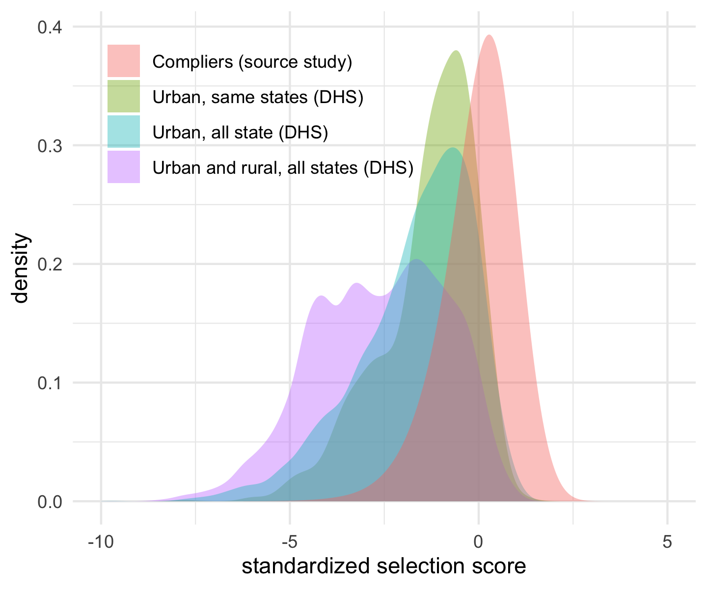
Figure 3: Estimated standardized selection score as a function of baseline covariates among four populations: (1) compliers in the source study, and (2) all women residing in urban areas in the 5 states represented in the source study, (3) all women residing in urban areas, and (4) all women in Nigeria.

To gauge the possible impact of the lack of overlap, we flag women with selection scores lower than the value of the fifth percentile in the source (-1.7) and re-compute the PATE by (i) excluding that group of women, and (ii) assuming there is no effect of contraceptive use on employment among them. The resulting PATEs are included in Table 4. Focusing on women more similar to the ones in the source study does not change the originally estimated effect, only increases the precision. When assuming a null effect for dissimilar women, the estimated PATE decreases as we target populations more distant from the source study, but remains positive. In order to nullify the estimated PATE we would need to entertain adverse effects of contraceptive use on employment for the women in the target population with combinations of characteristics poorly represented in the source study.

Table 4: PATE for different target populations, assuming different effects for women with combination of baseline characteristics not well represented among compliers in the source study.

	Proportion of women underrepresented in the target population	PATE excluding underrepresented women	PATE assuming no effect among underrepresented women
Urban, same states	0.337	.560 (.139)	0.392 (0.103)
Urban, all states	0.444	.528 (.129)	0.306 (0.076)
Urban and rural, all states	0.670	.564 (.130)	0.190 (0.045)

6.2.2 Sensitivity to confounding

Figure 4 presents the relation between the estimated PATE and population prevalence of a strong confounder. The findings suggest that a strong confounder should be present in at least 40% of the target population, for the 95% CI of the PATE to include zero. Confounder prevalence needs to exceed 80% for the 95% CI to be centered around zero.

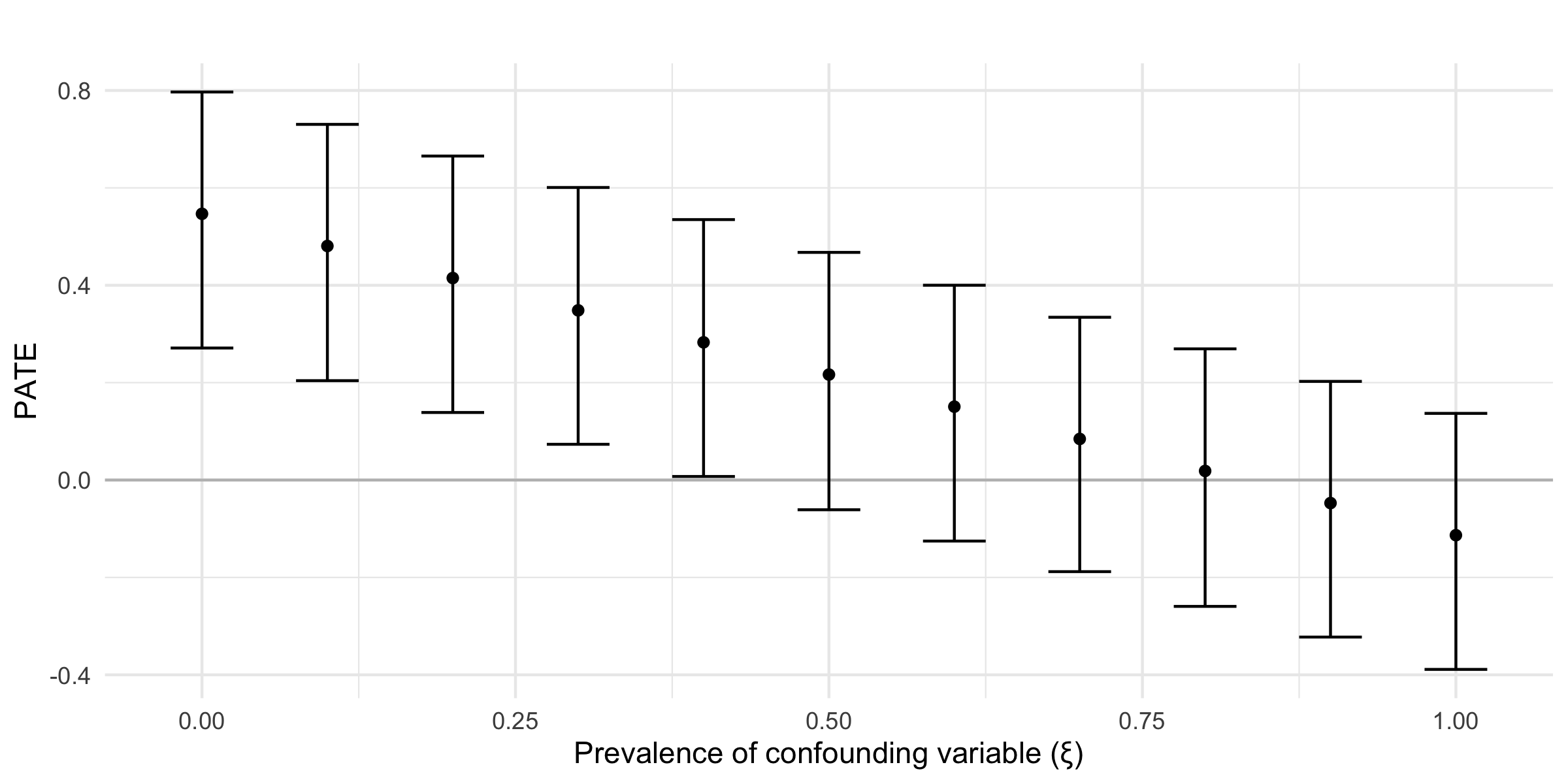
Figure 4: Sensitivity of the PATE to population prevalence of a strong of effect modifier.

Figure 5 presents the sensitivity of the PATE to a shift in the covariate distribution (between source and target) induced by an unobserved effect modifier. For the PATE’s CI to include zero, the ratio $\Gamma$ of the densities of the unmeasured covariate can be larger than 2.7. That is, if the unmeasured confounder is binary, the confounder can be more than two and a half times more prevalent in the target as compared to the source population for there still to be a positive effect.

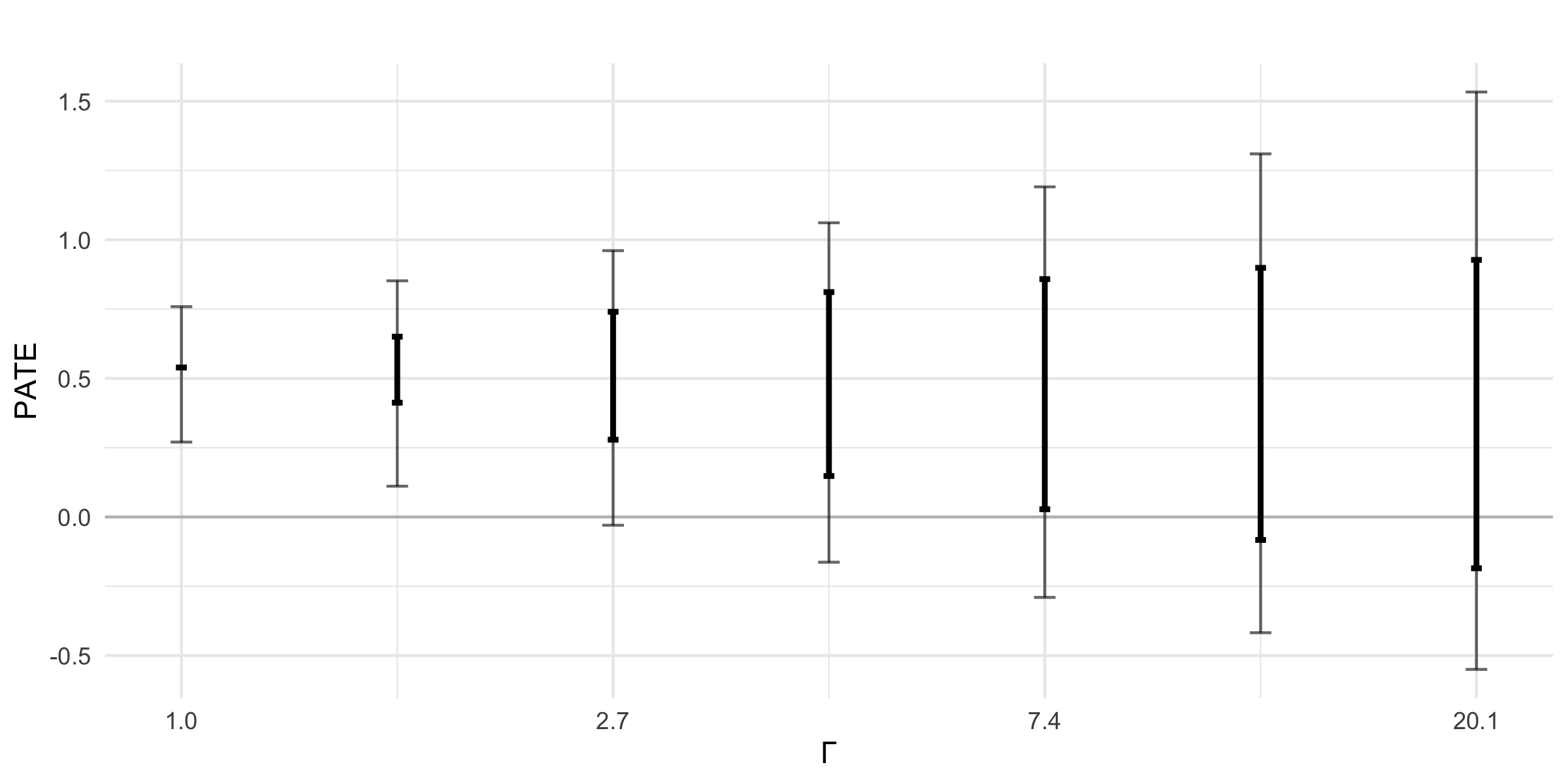
Figure 5: Sensitivity of the PATE to shift in the covariate distribution (between source and target) induced by an unobserved effect modifier (under a flexible non-parametric model for U). The x-axis quantifies the assumed bound on unobserved distributional shift (plotted on log-transformed scale). The dark gray represents the mean of the posterior distribution of the boundaries, the light gray the 95% credible intervals.

7 Discussion

Estimates of a causal effect of interest (such as the effect of adoption of modern contraception on employment) are frequently obtained from samples that are not representative of the population of interest. Participation in these studies -or compliance with the treatment assignment- is voluntary and may result in very selective samples. Our study draws on the growing body of work dealing with how to generalize from a selective sample to a larger population of interest (e.g., Degtiar and Rose (2023); Colnet et al. (2023)).

A frequent assumption that enables such generalization, is that all effect modifiers are observed -i.e., in our application, if women in the target population with the same observed characteristics as those in the source study were to adopt modern contraception, the effect would be approximately the same. Under that assumption, we used conditional average treatment effects (CATEs) obtained from the source population to estimate the population average treatment effect (PATE) for the target population. The approach requires estimates of the conditional effect (i.e., the. effect as a function of covariates) as an input from the source study but it is not limited to source studies using principal stratification or instrumental variables for identification.

We used a scaled Bayesian bootstrap approach to estimate the covariate distribution in the target population. This approach minimizes parametric assumptions, acknowledges estimation uncertainty, and considers the complex sampling design, which is common in practice. We show through simulation that a scaled BB procedure has good performance under repeated sampling that mimics the DHS complex sampling design.

In our application, we found that the average effect of adopting modern contraception in the target population is appreciably higher than in the source study based on point estimates, albeit the 95% credible intervals (CI) largely overlap. Robustness checks allowed us to identify some lack of overlap between the distribution of covariates, which increased considerably if the target population included women residing in rural areas. We examined the sensitivity of the results to the presence of an unobserved effect modifier with two different underlying models for the omitted variable. Both approaches suggested that a rather large imbalance in this hypothetical omitted variable would be required to explain away the effect in the population.

Findings should be interpreted considering the limitations of the study. We consider only DHS sampling design (stratified two-stage cluster sampling), which is commonly used in large demographic representative studies, but by no means the only one. Additional adaptation of the BB design has been proposed in the survey research literature and could be used for causal inference. Regarding the scope, the study does not address how the adoption of contraceptives occurs in the population of interest, if at all. At least for some women, that may require additional FP intervention that could enable or support that change.

In sum, we have introduced a strategy to generalize causal effects obtained from a population that may differ systematically from the population of interest, using information from a complex sample to estimate the distribution of effect modifiers in the target population. We have also showed multiple ways to check the robustness of the results when not all effect modifiers have been addressed.

[Acknowledgments] The authors would like to thank Jocelyn Finlay, Jonathan Bearak, Matt Hamilton, Onikepe Owolabi, Jennifer Seager, and John Stover, as well as Aaron Leor Sarvet, Ted Westling and Nicholas Reich for helpful comments on this work. This paper is a product of the investigator’s work within the Family Planning Impact Consortium: a multi-disciplinary partnership between the Guttmacher Institute, African Institute for Development Policy, Avenir Health, Institute for Disease Modeling of the Gates Foundation’s Global Health Division, with investigators at the University of Massachusetts Amherst, the University of North Carolina, the George Washington University, and the Institut Supérieur des Sciences de la Population de l’Université Joseph Ki-Zerbo. The Consortium seeks to generate robustestimates of how family planning affects a range of social and economic domains across the life course. Members of the Consortium have developed unique model-based approaches to generating evidence that examines relationships between family planning and empowerment-related variables. Code used for this article is available at https://github.com/AlkemaLab/general_Bayes This paper was made possible by grants from the Bill & Melinda Gates Foundation and the Children’s Investment Fund Foundation, who support the work of the Family Planning Impact Consortium. The findings and conclusions contained within do not necessarily reflect the positions or policies of the donors. Additional Funder information: Funder: Bill & Melinda Gates Foundation, Award Number: INV-018349, Grant Recipient: Guttmacher Institute; Funder: Children’s Investment Fund Foundation, Award Number: 2012-05769, Grant Recipient: Guttmacher Institute.

Appendices The supplement includes the definition of the target population in terms of DHS variables (Appendix I), additional characteristics for compliers and target population (Appendix II), and additional simulation results (Appendix III).

References

- Aitkin (2008) {barticle}[author] \bauthor\bsnmAitkin, \bfnmM.\binitsM. (\byear2008). \btitleApplications of the Bayesian Bootstrap in Finite Population Inference. \bjournalJournal of Official Statistics \bvolume24 \bpages21–51. \endbibitem
- Angrist and Fernandez-Val (2010) {bbook}[author] \bauthor\bsnmAngrist, \bfnmJ.\binitsJ. and \bauthor\bsnmFernandez-Val, \bfnmI.\binitsI. (\byear2010). \btitleExtrapoLATE-ing: External Validity and Overidentification in the LATE Framework. \bpublisherNational Bureau of Economic Research \bnotew16566. \bdoi10.3386/w16566 \endbibitem
- Aronow and Carnegie (2013) {barticle}[author] \bauthor\bsnmAronow, \bfnmP. M.\binitsP. M. and \bauthor\bsnmCarnegie, \bfnmA.\binitsA. (\byear2013). \btitleBeyond LATE: Estimation of the Average Treatment Effect with an Instrumental Variable. \bjournalPolitical Analysis \bvolume21 \bpages492–506. \bdoi10.1093/pan/mpt013 \endbibitem
- Chamberlain and Imbens (2003) {barticle}[author] \bauthor\bsnmChamberlain, \bfnmG.\binitsG. and \bauthor\bsnmImbens, \bfnmG. W.\binitsG. W. (\byear2003). \btitleNonparametric Applications of Bayesian Inference. \bjournalJournal of Business & Economic Statistics \bvolume21 \bpages12–18. \bdoi10.1198/073500102288618711 \endbibitem
- Chipman, George and McCulloch (2010) {barticle}[author] \bauthor\bsnmChipman, \bfnmH. A.\binitsH. A., \bauthor\bsnmGeorge, \bfnmE. I.\binitsE. I. and \bauthor\bsnmMcCulloch, \bfnmR. E.\binitsR. E. (\byear2010). \btitleBART: Bayesian additive regression trees. \bjournalThe Annals of Applied Statistics \bvolume4 \bpages266–298. \bdoi10.1214/09-AOAS285 \endbibitem
- Cohen (1997) {binproceedings}[author] \bauthor\bsnmCohen, \bfnmM.\binitsM. (\byear1997). \btitleThe Bayesian bootstrap and multiple imputation for unequal probability sample designs. In \bbooktitleProceedings of the Survey Research Methods Section. American Statistical Association. \endbibitem
- Colnet et al. (2022) {barticle}[author] \bauthor\bsnmColnet, \bfnmB.\binitsB., \bauthor\bsnmJosse, \bfnmJ.\binitsJ., \bauthor\bsnmVaroquaux, \bfnmG.\binitsG. and \bauthor\bsnmScornet, \bfnmE.\binitsE. (\byear2022). \btitleReweighting the RCT for generalization: Finite sample error and variable selection. \bjournalarXiv. \endbibitem
- Colnet et al. (2023) {barticle}[author] \bauthor\bsnmColnet, \bfnmB.\binitsB., \bauthor\bsnmMayer, \bfnmI.\binitsI., \bauthor\bsnmChen, \bfnmG.\binitsG., \bauthor\bsnmDieng, \bfnmA.\binitsA., \bauthor\bsnmLi, \bfnmR.\binitsR., \bauthor\bsnmVaroquaux, \bfnmG.\binitsG., \bauthor\bsnmVert, \bfnmJ. P.\binitsJ. P., \bauthor\bsnmJosse, \bfnmJ.\binitsJ. and \bauthor\bsnmYang, \bfnmS.\binitsS. (\byear2023). \btitleCausal inference methods for combining randomized trials and observational studies: A review. \bjournalarXiv. \endbibitem
- Corsi et al. (2012) {barticle}[author] \bauthor\bsnmCorsi, \bfnmD. J.\binitsD. J., \bauthor\bsnmNeuman, \bfnmM.\binitsM., \bauthor\bsnmFinlay, \bfnmJ. E.\binitsJ. E. and \bauthor\bsnmSubramanian, \bfnmS.\binitsS. (\byear2012). \btitleDemographic and health surveys: A profile. \bjournalInternational Journal of Epidemiology \bvolume41 \bpages1602–1613. \bdoi10.1093/ije/dys184 \endbibitem
- Degtiar and Rose (2023) {barticle}[author] \bauthor\bsnmDegtiar, \bfnmI.\binitsI. and \bauthor\bsnmRose, \bfnmS.\binitsS. (\byear2023). \btitleA Review of Generalizability and Transportability. \bjournalAnnual Review of Statistics and Its Application \bvolume10. \bdoi10.1146/annurev-statistics-042522-103837 \endbibitem
- Dong, Elliott and Raghunathan (2014) {barticle}[author] \bauthor\bsnmDong, \bfnmQ.\binitsQ., \bauthor\bsnmElliott, \bfnmM. R.\binitsM. R. and \bauthor\bsnmRaghunathan, \bfnmT. E.\binitsT. E. (\byear2014). \btitleA nonparametric method to generate synthetic populations to adjust for complex sampling design features. \bjournalSurvey Methodology \bvolume40 \bpages29–46. \endbibitem
- Garraza, Speizer and Alkema (2024) {barticle}[author] \bauthor\bsnmGarraza, \bfnmL. G.\binitsL. G., \bauthor\bsnmSpeizer, \bfnmI.\binitsI. and \bauthor\bsnmAlkema, \bfnmL.\binitsL. (\byear2024). \btitleCombining BART and Principal Stratification to estimate the effect of intermediate on primary outcomes with application to estimating the effect of family planning on employment in sub-Saharan Africa. \bjournalarXiv. \endbibitem
- Hernán and Robins (2006) {barticle}[author] \bauthor\bsnmHernán, \bfnmM. A.\binitsM. A. and \bauthor\bsnmRobins, \bfnmJ. M.\binitsJ. M. (\byear2006). \btitleInstruments for Causal Inference: An Epidemiologist’s Dream? \bjournalEpidemiology \bvolume17 \bpages360–372. \bdoi10.1097/01.ede.0000222409.00878.37 \endbibitem
- Hill (2011) {barticle}[author] \bauthor\bsnmHill, \bfnmJ. L.\binitsJ. L. (\byear2011). \btitleBayesian Nonparametric Modeling for Causal Inference. \bjournalJournal of Computational and Graphical Statistics \bvolume20 \bpages217–240. \bdoi10.1198/jcgs.2010.08162 \endbibitem
- Li, Ding and Mealli (2022) {barticle}[author] \bauthor\bsnmLi, \bfnmF.\binitsF., \bauthor\bsnmDing, \bfnmP.\binitsP. and \bauthor\bsnmMealli, \bfnmF.\binitsF. (\byear2022). \btitleBayesian Causal Inference: A Critical Review. \bjournalarXiv. \endbibitem
- Little (2014) {bincollection}[author] \bauthor\bsnmLittle, \bfnmR. J. A.\binitsR. J. A. (\byear2014). \btitleSurvey sampling: Past controversies, current orthodoxy, and future paradigm. In \bbooktitlePast, Present, and Future of Statistical Science (\beditor\bfnmX.\binitsX. \bsnmLin, \beditor\bfnmC.\binitsC. \bsnmGenest, \beditor\bfnmD. L.\binitsD. L. \bsnmBanks, \beditor\bfnmG.\binitsG. \bsnmMolenberghs, \beditor\bfnmD. W.\binitsD. W. \bsnmScott and \beditor\bfnmJ. L.\binitsJ. L. \bsnmWang, eds.) \bpublisherChapman and Hall/CRC. \bdoi10.1201/b16720 \endbibitem
- Lo (1988) {barticle}[author] \bauthor\bsnmLo, \bfnmA. Y.\binitsA. Y. (\byear1988). \btitleA Bayesian Bootstrap for a Finite Population. \bjournalThe Annals of Statistics \bvolume16. \bdoi10.1214/aos/1176351061 \endbibitem
- Lumley (2020) {bmanual}[author] \bauthor\bsnmLumley, \bfnmT.\binitsT. (\byear2020). \btitlesurvey: Analysis of complex survey samples \bnoteVersion R package version 4.0. \endbibitem
- Makela, Si and Gelman (2018) {barticle}[author] \bauthor\bsnmMakela, \bfnmS.\binitsS., \bauthor\bsnmSi, \bfnmY.\binitsY. and \bauthor\bsnmGelman, \bfnmA.\binitsA. (\byear2018). \btitleBayesian inference under cluster sampling with probability proportional to size. \bjournalStatistics in Medicine \bvolume37 \bpages3849–3868. \bdoi10.1002/sim.7892 \endbibitem
- Nie, Imbens and Wager (2021) {barticle}[author] \bauthor\bsnmNie, \bfnmX.\binitsX., \bauthor\bsnmImbens, \bfnmG.\binitsG. and \bauthor\bsnmWager, \bfnmS.\binitsS. (\byear2021). \btitleCovariate Balancing Sensitivity Analysis for Extrapolating Randomized Trials across Locations. \bjournalarXiv. \endbibitem
- NPC and ICF (2019) {bmanual}[author] \bauthor\bsnmNPC, \bfnmNational Population Commission\binitsN. P. C. and \bauthor\bsnmICF (\byear2019). \btitleNigeria Demographic and Health Survey 2018—Final Report. \endbibitem
- Oganisian, Mitra and Roy (2022) {barticle}[author] \bauthor\bsnmOganisian, \bfnmA.\binitsA., \bauthor\bsnmMitra, \bfnmN.\binitsN. and \bauthor\bsnmRoy, \bfnmJ.\binitsJ. (\byear2022). \btitleHierarchical Bayesian Bootstrap for Heterogeneous Treatment Effect Estimation. \bjournalThe International Journal of Biostatistics \bvolume0. \bdoi10.1515/ijb-2022-0051 \endbibitem
- Rao and Wu (2010) {barticle}[author] \bauthor\bsnmRao, \bfnmJ. N. K.\binitsJ. N. K. and \bauthor\bsnmWu, \bfnmC.\binitsC. (\byear2010). \btitleBayesian Pseudo-Empirical-Likelihood Intervals for Complex Surveys. \bjournalJournal of the Royal Statistical Society Series B: Statistical Methodology \bvolume72 \bpages533–544. \bdoi10.1111/j.1467-9868.2010.00747.x \endbibitem
- Rosenbaum and Rubin (1983) {barticle}[author] \bauthor\bsnmRosenbaum, \bfnmP. R.\binitsP. R. and \bauthor\bsnmRubin, \bfnmD. B.\binitsD. B. (\byear1983). \btitleThe central role of the propensity score in observational studies for causal effects. \bjournalBiometrika \bvolume70 \bpages41–55. \bdoi10.1093/biomet/70.1.41 \endbibitem
- Rubin (1981) {barticle}[author] \bauthor\bsnmRubin, \bfnmD. B.\binitsD. B. (\byear1981). \btitleThe Bayesian Bootstrap. \bjournalThe Annals of Statistics \bvolume9. \bdoi10.1214/aos/1176345338 \endbibitem
- Rudolph and Laan (2017) {barticle}[author] \bauthor\bsnmRudolph, \bfnmK. E.\binitsK. E. and \bauthor\bsnmLaan, \bfnmM. J.\binitsM. J. (\byear2017). \btitleRobust Estimation of Encouragement Design Intervention Effects Transported Across Sites. \bjournalJournal of the Royal Statistical Society Series B: Statistical Methodology \bvolume79 \bpages1509–1525. \bdoi10.1111/rssb.12213 \endbibitem
- Stuart et al. (2011) {barticle}[author] \bauthor\bsnmStuart, \bfnmE. A.\binitsE. A., \bauthor\bsnmCole, \bfnmS. R.\binitsS. R., \bauthor\bsnmBradshaw, \bfnmC. P.\binitsC. P. and \bauthor\bsnmLeaf, \bfnmP. J.\binitsP. J. (\byear2011). \btitleThe Use of Propensity Scores to Assess the Generalizability of Results from Randomized Trials. \bjournalJournal of the Royal Statistical Society Series A: Statistics in Society \bvolume174 \bpages369–386. \bdoi10.1111/j.1467-985X.2010.00673.x \endbibitem
- Taddy et al. (2016) {barticle}[author] \bauthor\bsnmTaddy, \bfnmM.\binitsM., \bauthor\bsnmGardner, \bfnmM.\binitsM., \bauthor\bsnmChen, \bfnmL.\binitsL. and \bauthor\bsnmDraper, \bfnmD.\binitsD. (\byear2016). \btitleA Nonparametric Bayesian Analysis of Heterogenous Treatment Effects in Digital Experimentation. \bjournalJournal of Business & Economic Statistics \bvolume34 \bpages661–672. \bdoi10.1080/07350015.2016.1172013 \endbibitem
- Wang and Tchetgen Tchetgen (2018) {barticle}[author] \bauthor\bsnmWang, \bfnmL.\binitsL. and \bauthor\bsnmTchetgen Tchetgen, \bfnmE.\binitsE. (\byear2018). \btitleBounded, Efficient and Multiply Robust Estimation of Average Treatment Effects Using Instrumental Variables. \bjournalJournal of the Royal Statistical Society Series B: Statistical Methodology \bvolume80 \bpages531–550. \bdoi10.1111/rssb.12262 \endbibitem
- Wang et al. (2015) {barticle}[author] \bauthor\bsnmWang, \bfnmC.\binitsC., \bauthor\bsnmDominici, \bfnmF.\binitsF., \bauthor\bsnmParmigiani, \bfnmG.\binitsG. and \bauthor\bsnmZigler, \bfnmC. M.\binitsC. M. (\byear2015). \btitleAccounting for uncertainty in confounder and effect modifier selection when estimating average causal effects in generalized linear models. \bjournalBiometrics \bvolume71 \bpages654–665. \bdoi10.1111/biom.12315 \endbibitem
- Xu, Daniels and Winterstein (2018) {barticle}[author] \bauthor\bsnmXu, \bfnmD.\binitsD., \bauthor\bsnmDaniels, \bfnmM. J.\binitsM. J. and \bauthor\bsnmWinterstein, \bfnmA. G.\binitsA. G. (\byear2018). \btitleA Bayesian Nonparametric Approach to Causal Inference on Quantiles. \bjournalBiometrics \bvolume74 \bpages986–996. \bdoi10.1111/biom.12863 \endbibitem
- Zangeneh and Little (2015) {barticle}[author] \bauthor\bsnmZangeneh, \bfnmS. Z.\binitsS. Z. and \bauthor\bsnmLittle, \bfnmR. J. A.\binitsR. J. A. (\byear2015). \btitleBayesian Inference for the Finite Population Total from a Heteroscedastic Probability Proportional to Size Sample. \bjournalJournal of Survey Statistics and Methodology \bvolume3 \bpages162–192. \bdoi10.1093/jssam/smv002 \endbibitem