Dependence of convective precipitation extremes on near-surface relative humidity
Abstract
Precipitation extremes produced by convection have been found to intensify with near-surface temperatures at a Clausius-Clapeyron rate of to K-1 in simulations of radiative-convective equilibrium (RCE). However, these idealized simulations are typically performed over an ocean surface with a high near-surface relative humidity (RH) that stays roughly constant with warming. Over land, near-surface RH is lower than over ocean and is projected to decrease by global climate models. Here, we investigate the dependence of precipitation extremes on near-surface RH in convection-resolving simulations of RCE. We reduce near-surface RH by increasing surface evaporative resistance while holding free-tropospheric temperatures fixed by increasing surface temperature. This “top-down” approach produces an RCE state with a deeper, drier boundary layer, which weakens convective precipitation extremes in three distinct ways. First, the lifted condensation level is higher, leading to a small thermodynamic weakening of precipitation extremes. Second, the higher lifted condensation level also reduces positive buoyancy in the lower troposphere, leading to a dynamic weakening of precipitation extremes. Third, precipitation re-evaporates more readily when falling through a deeper, drier boundary layer, leading to a substantial decrease in precipitation efficiency. These three effects all follow from changes in near-surface relative humidity and are physically distinct from the mechanism that underpins the Clausius-Clapeyron scaling rate. Overall, our results suggest that changes in relative humidity must be taken into account when seeking to understand and predict changes in convective precipitation extremes over land.
Thunderstorms and other types of convection produce very heavy rainfall in many regions on Earth. In this paper, we ran a computer model to show that when relative humidity near the surface is reduced, convection produces weaker rainfall rates. This happens for three reasons: the updrafts in the storms are weaker, there is less cloud-water because the cloud base is higher, and less of that cloud-water makes it to the surface as rainfall. This is an important finding because we expect that relative humidity will decrease over many land regions as the climate warms, possibly seasonally offsetting some of the impact on rainfall extremes of increases in the absolute amount of water vapor.
1 Introduction
The heaviest of precipitation events are affected by climate change through a “thermodynamic contribution” related to increasing water vapor, a “dynamic” contribution related to changes in vertical velocities, and by changes in “precipitation efficiency,” the fraction of condensed water vapor that actually reaches the surface as precipitation (O’Gorman, 2015). For convective precipitation extremes, the thermodynamic contribution approximately follows a Clausius-Clapeyron scaling rate of to per K of surface warming (Muller et al., 2011; Romps, 2011; Abbott et al., 2020). Precipitation extremes scale near the Clausius-Clapeyron rate in global climate model (GCM) projections at the global scale, albeit with large uncertainties in the tropics (e.g., O’Gorman and Schneider, 2009; Kharin et al., 2013), in some regional studies with convection-resolving models (CRMs) (e.g., Ban et al., 2015; Prein et al., 2017), and in globally-aggregated observations over land (Westra et al., 2013). Evidence exists, however, from observations (Fowler et al., 2021), GCM projections (Pfahl et al., 2017; Williams and O’Gorman, 2022), and regional CRM studies (Lenderink et al., 2021) that precipitation extremes may regionally and seasonally respond to climate change at a rate that deviates from Clausius-Clapeyron scaling.
Williams and O’Gorman (2022), in particular, found a seasonal contrast in the scaling rates of precipitation extremes with climate warming across simulations from the Coupled Model Intercomparison Project, Phase 5 (CMIP5) (Taylor et al., 2012). They found that over midlatitude land in the Northern Hemisphere, dynamic contributions to precipitation extremes were near-zero in the winter but negative in the summer. This negative dynamic contribution is likely related to convection, since convective precipitation extremes are common in the summer. Williams and O’Gorman (2022) further found a correlation between these summertime negative dynamical contributions and a decrease in summertime near-surface relative humidity (RH), suggesting that convective precipitation extremes respond dynamically to decreases in near-surface RH.
Near-surface RH is often thought to influence precipitation extremes and their response to climate change through the Clausius-Clapeyron rate. Only when RH stays constant will near-surface specific humidity scale one-to-one with saturation specific humidity and follow the Clausius-Clapeyron rate. With this in mind, a number of papers have opted to scale precipitation extremes against dew-point temperature instead of temperature, arguing that a direct measure of atmospheric moisture content should produce a scaling, absent other effects, that follows the Clausius-Clapeyron rate (Lenderink and van Meijgaard, 2010; Lenderink et al., 2011; Lepore et al., 2015; Barbero et al., 2018; Lenderink et al., 2021). However, arguments in favor of such a “dew-point scaling” approach over a more traditional “temperature scaling” implicitly assume that RH only matters for its influence on the thermodynamic contribution to changes in precipitation extremes. By finding a relationship between RH and a dynamic contribution, Williams and O’Gorman (2022) have called this assumption into question.
Near-surface RH is expected to decrease over land in response to anthropogenic climate change for several reasons. First, RH is expected to decrease over land because water vapor over land is influenced by moisture transport from over ocean, while at the same time ocean warming is weaker than the land warming. Thus, the source of water vapor from over ocean can’t keep pace with the increasing saturation vapor pressure over land (Simmons et al., 2010; Byrne and O’Gorman, 2016, 2018). In addition, surface evapotranspiration rates provide a direct control on near-surface RH. Surface evapotranspiration and thus near-surface RH is reduced by a “physiological forcing” in which plant stomata close in response to higher atmospheric CO2 levels (Cao et al., 2010), and this stomatal closure has been found to decrease mean precipitation in summer over the northern midlatitudes (Skinner et al., 2017). Lastly, decreases in soil moisture are also expected to influence near-surface RH (Berg et al., 2016; Zhou et al., 2023). Comparison between observed and simulated trends in RH in recent decades shows that GCMs underestimate decreases in near-surface RH in arid and semi-arid regions (Simpson et al., 2024), which means that they may also underestimate any resulting impacts on precipitation in these regions.
In this paper, we investigate the sensitivity of convective precipitation extremes to near-surface RH in the simplest possible setting: a CRM run to a state of radiative-convective equilibrium (RCE). In regional simulations, across a wide range of relative humidities, CRMs have been demonstrated to reproduce observed precipitation extremes more reliably than models that use convective parameterizations (Lenderink et al., 2024). In RCE simulations, CRMs are additionally useful because they allow for careful, controlled study of the physics underlying precipitation statistics and their response to different climate forcings. A number of studies of idealized CRM simulations of RCE have found that convective precipitation extremes scale quite close to the Clausius-Clapeyron rate in response to warming (Muller et al., 2011; Romps, 2011). Dynamic contributions to precipitation extremes remain relatively small in these idealized studies, even when convection is organized into squall lines by wind shear (Muller, 2013) or overturning structures in a channel domain (Abbott et al., 2020). These particular studies also did not find large changes in precipitation efficiency, but Singh and O’Gorman (2014) did find that precipitation efficiency decreased in colder RCE states due to microphysical effects. Several other idealized CRM studies have diagnosed the importance of various physical processes in setting the precipitation efficiency for both mean and extreme precipitation (Lutsko and Cronin, 2018; Da Silva et al., 2021; Abramian et al., 2023; Langhans et al., 2015). However, the RCE studies cited above have all used an ocean surface as a bottom boundary condition, and so the influence of near-surface RH on precipitation extremes in states of RCE has remained relatively unexplored.
We are aware of two CRM studies of the effect of overall surface dryness on convective intensity in RCE: Hansen and Back (2015) and Sarbeng (2023). These studies were motivated by observational evidence that convection is more intense over land than over ocean (Zipser et al., 2006). Both studies found that the maximum updraft velocity does not increase with a higher Bowen ratio (less evaporative surface), which suggests that the land-ocean contrast in convective intensity is not due to the contrast in surface dryness. Sarbeng (2023) even found weakening in updrafts in the lower free troposphere as the surface dries, which could be consistent with the negative dynamic contribution to precipitation extremes found by Williams and O’Gorman (2022) in response to lower near-surface RH, especially given that condensation rates are sensitive to updraft velocities in the lower troposphere where saturation vapor pressures are relatively high.
To modify near-surface RH in our simulations, we introduce a “vegetative” evaporative resistance parameter similar to Betts (2000) and inspired by the effects of stomatal closure on surface relative humidity. As the climate changes, decreases in near-surface RH occur alongside increases in near-surface temperatures, such that the near-surface moist static energy and free-tropospheric temperatures (which are convectively coupled at equilibrium and under the influence of larger-scale dynamics) tend not to change as much (e.g., Byrne and O’Gorman, 2013; Berg et al., 2016). Thus we follow the general approach of Hansen and Back (2015) and Sarbeng (2023) by holding the free-tropospheric temperature fixed as the surface dries, specifically using the relaxation procedure introduced by Sarbeng (2023). For simplicity, we do not parameterize the effects of changes in large-scale dynamics or include the diurnal cycle, both of which should be considered in future work.
Section 2 describes the vegetative resistance parameter, the relaxation procedure, and the model simulations more generally. Section 3 presents an overview of the mean RCE state achieved by varying the vegetative resistance and the fundamental result of this paper: that precipitation extremes vary substantially with near-surface RH, and that the mechanisms involves changes in dynamics and precipitation efficiency rather than the thermodynamic contribution that gives rise to the Clausius-Clapeyron scaling rate of precipitation extremes. Sections 4 and 5 explain this dependence in more detail. Specifically, Section 4 shows that a higher lifted condensation level weakens convective updrafts in the lower troposphere, while Section 5 diagnoses changes in precipitation efficiency in terms of cloud microphysics and re-evaporation. Section 6 provides a concluding discussion, highlighting the implications of a large sensitivity of precipitation extremes to near-surface RH.
2 Model and simulations
2.1 Convection-resolving model and basic setup
We use the System for Atmospheric Modeling (SAM), version 6.11 (Khairoutdinov and Randall, 2003). All simulations were run with a km horizontal grid spacing in a km2 domain, and with vertical levels. Vertical spacing starts at m near the surface and increased steadily until the model top at a height of km. Above km, atmospheric motions are damped in a sponge layer. SAM was run with its own one-moment microphysics parameterization. No diurnal cycle was simulated; instead, a constant zenith angle of was used. This zenith angle, along with a solar constant set to W/m2, produces Earth’s equatorial annual average of insolation weighted by the cosine zenith angle, following the recommendations of Cronin (2014).
2.2 Vegetative evaporative resistance and surface temperature
We modify near-surface RH by altering the rate of surface evaporation. To accomplish this, a free parameter, the “vegetative resistance” , was introduced in SAM’s equation for the surface latent heat flux:
| (1) |
where is near-surface air density, is the latent heat of vaporization, is the difference between near-surface mixing ratio and the saturation mixing ratio at surface (skin) temperature , and is an “aerodynamic resistance.” For the aerodynamic resistance, is a unitless exchange coefficient determined by Monin-Obukhov similarity theory and is the near-surface windspeed. When calculating surface heat fluxes, SAM sets to have a minimum value of m s-1 to account for unresolved gusts.
We model the surface to be horizontally homogeneous, so that there are no spatial variations in or in the surface temperature . The surface is an ocean when s m-1 and surface evaporation rates decrease as is increased (all else held equal). Modifications to evaporation through affect the surface energy budget, and so may not stay constant as is varied. An intuitive approach to determining a value for , given a value of , is to simply to solve the surface energy budget until equilibrium is achieved, as has been done by some past RCE studies (e.g., Romps (2011)). Simulations using this approach (not shown) reached a state of equilibrium with lower at large , causing the free troposphere to cool substantially.111As increased, the free troposphere in these simulations dried and cooled in order to maintain the same outgoing longwave radiation. This kind of radiative response to (and similar parameters) has been found previously in GCM studies that varied evaporation rates via fractional coverage of land continents vs. ocean (Laguë et al., 2021, 2023). Such a free-tropospheric cooling is inconsistent with the constraint of weak temperature gradients (WTG) in the tropics. Instead, we take a “top-down” perspective on the controls on land temperatures at climate equilibrium, which argues that free-tropospheric temperatures over land are strongly coupled vertically to surface temperature and moisture in convecting regions by moist adiabatic lapse rates, and also strongly coupled horizontally to free-tropospheric temperatures over ocean by horizontal advection and gravity wave dynamics. This perspective has previously been used to explain the land-ocean warming and moistening contrasts under climate change (e.g., Joshi et al., 2008; Byrne and O’Gorman, 2013), and it implies that free-tropospheric temperatures over land should not necessarily change in response to a change in surface evapotranspiration.
With this perspective in mind, we use a method devised by Sarbeng (2023), which adjusts so that horizontal-mean temperature is nudged towards a reference profile within a specified pressure layer between and . That is, we evolve forward in time using
| (2) |
where is the thickness of the layer and is a relaxation timescale. This implementation differs from Sarbeng (2023) in two ways. First, the integral was evaluated in pressure coordinates, not height coordinates, with hPa and hPa. Second, a longer relaxation timescale of days was used instead of hr. Both of these modifications dampened oscillations in that appeared in initial attempts to apply this adjustment. The reference profile was calculated from a simulation with as described in the next subsection.
An alternative approach would be to parameterize WTG dynamics by introducing a large-scale vertical velocity that prevents large changes in free-tropospheric temperature (Sobel and Bretherton, 2000; Raymond and Zeng, 2005). The role of changes in large-scale vertical velocities is an important topic for future work, but here we focus on the simplest case of RCE.
2.3 Simulations
In total, simulations were run. Each simulation is associated with a different vegetative resistance : , , , , and s m-1. The same reference profile was used to determine a surface temperature for each simulation. The reference profile was calculated by first running SAM in an “ocean RCE” configuration: s m-1 and K. This ocean RCE simulation was run for 50 days, and was calculated by averaging horizontally and over the last 10 days of the simulation.
Once was determined, the following procedure was used for every simulation (including s m-1). First, SAM was run for days, with evolved forward in time following Equation (2). If, averaged horizontally and over the last days of this simulation, the vertical average between and of temperature and the reference profile were within K, then the average value of over those days was saved. Otherwise, the simulation was run for more days and the procedure was repeated. Once a value of was saved, SAM was re-run from rest with this fixed value of for days. The last days of those fixed- simulations were used for all of the analysis presented below; during this day period, instantaneous snapshots from SAM were saved every hours. Table 1 reports the equilibrium values of , as well as the horizontal- and time-average near-surface temperature, near-surface RH, near-surface , and surface precipitation rates for all simulations. The values of were spaced further apart at large values of , so that for each increment in , increased by approximately K and RH decreased by approximately (Table 1).
| (s m) | (K) | near-sfc (K) | near-sfc RH (%) | near-sfc (g kg) | (mm day-1) |
|---|---|---|---|---|---|
3 Response to changes in surface dryness
3.1 Response of mean climate
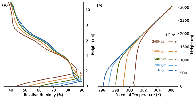
As increases, the boundary layer changes in three ways. First, near-surface RH and specific humidity decrease with increasing (Table 1 and Fig. 1a). Second, temperatures increase in the boundary layer even as temperature stays constant in the free troposphere (Table 1 and Fig. 1b). Third, the lifted condensation level (LCL), calculated analytically (Romps, 2017) using horizontal- and time-mean near-surface air properties, rises as increases (Fig. 1b). If we consider the s m-1 simulation as “ocean” and the s m-1 simulations as “land,” then these tendencies are consistent with the top-down perspective on land-ocean contrasts of Byrne and O’Gorman (2013) (c.f. their Fig. 1), since the surface temperature over land must be higher given the same free-tropospheric temperatures over land and ocean, moist- adiabatic lapse rates above the LCL and dry adiabatic lapse rates below the LCL, and a higher LCL over land. One difference is that lapse rates below the LCL in our simulations shown in Fig. 1b are not quite dry adiabatic because of precipitation-driven cold pools.
The reference temperature profile, , calculated over an ocean surface ( s/m), is closely followed through the free troposphere in simulations with s/m. Thus, in conjunction with the relaxation procedure, acts as a control on the near-surface RH without modifying free-tropospheric temperatures. Relative humidity also decreases somewhat in the free troposphere with increasing .
3.2 Response of precipitation extremes
Every horizontal gridpoint and time in a given simulation has its own value of the instantaneous precipitation rate (saved directly) and the vertically-integrated condensation rate (calculated as described below from Equation (3)). We characterize extreme precipitation by the average of over all values at and above the th percentile of . Similarly, extreme condensation is the average of over all values at and above the th percentile of . Precipitation efficiency is defined as the ratio , and thus involves different sets of gridpoints and times for and , following the approach of Singh and O’Gorman (2014), Abbott et al. (2020), and Da Silva et al. (2021) which recognizes that the different variables peak at different points in the convective lifecycle.
We find that precipitation extremes weaken substantially as the surface dries and RH decreases (Fig. 2). When increases from s m-1 to s m-1, precipitation extremes decrease from mm hr-1 to mm hr-1 (Fig. 2a), a fractional decrease. Over the same range of , near-surface RH decreases from to (Fig. 2b). This is an absolute decrease in RH of percentage points (pt), or a fractional decrease of . Thus, we calculate (following the methodology described in Section 33.3) the scaling rate between our wettest and driest simulations either as a per pt (absolute) increase in RH or as a per (fractional) increase in RH. This scaling rate is the same sign as, but half the magnitude of, the roughly per scaling rate found by Williams and O’Gorman (2022) for the dynamical contribution to changes in precipitation extremes over northern hemisphere midlatitude land in the summertime (c.f. their Fig. 3).
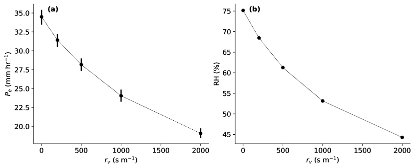
Note that this scaling rate is computed between simulations with a large difference in RH. The scaling rate against absolute changes in RH is smaller over wetter surfaces ( per pt between s m-1 and s m-1) and larger over drier surfaces ( per pt between s m-1 and s m-1). In contrast, the scaling rate against fractional changes in RH varies less between wetter surfaces ( per between s m-1 and s m-1) vs. drier surfaces ( per between s m-1 and s m-1). Given this reduced variability, we present our results in terms of scaling rates against fractional changes in RH across our full range of simulations (unless otherwise stated). This is also consistent with Williams and O’Gorman (2022), who report fractional changes in RH (A. Williams, 2024, personal communication).
Although we focus on precipitation extremes in this paper, we have also found that the fractional decrease in is nearly identical to a decrease, from mm day-1 to mm day-1, in the horizontal- and time-mean precipitation rate (Table 1). This is different from CRM and GCM simulations that either warm the surface or increase CO2 concentrations, which find that mean precipitation rates are energetically constrained to scale with warming below the CC scaling rate that precipitation extremes approximately follow (Allen and Ingram, 2002; heldsoden; O’Gorman and Schneider, 2009; Muller et al., 2011).
3.3 Decomposition of response of precipitation extremes
High percentile instantaneous surface precipitation rates are associated with deep convection wherein strong updrafts condense moisture. SAM does not explicitly calculate condensation rates, and we want to decompose changes in the condensation rate into contributions from different physical factors. Therefore, we calculate the column-integrated condensation rate as
| (3) |
where is the height of the LCL calculated following Romps (2017) using near-surface values of the column, km is a fixed upper height, is vertical velocity, is the updraft speed (i.e., excluding downdrafts), is the saturation mixing ratio (a function of only temperature and pressure ), and the subscript indicates that the derivative is calculated following a local moist adiabatic lapse rate. This definition of the condensation integral differs from the common definition (e.g., O’Gorman and Schneider, 2009). First, a lower bound of is used instead of . Second, is used instead of . Both of these choices are made on a physical basis: only upward velocities drive condensation, and convective clouds do not typically extend to the surface. The alternative choice of using instead of gives an approximate expression for net condensation (i.e., condensation from updrafts minus re-evaporation from downdrafts), but we include only updrafts so that the effect of re-evaporation is fully included in the precipitation efficiency. Also, given that the LCL rises with increasing (Fig. 1), it is important to diagnose the effect that the LCL has on condensation rates in order to correctly associate thermodynamic contributions, dynamic contributions, and changes in precipitation efficiency with the appropriate underlying mechanisms.
Letting denote the difference in a variable between two climate states and denote the average value of that variable between two climate states, then the relation allows for fractional changes in precipitation to be decomposed in terms of fractional changes in efficiency and condensation:
| (4) |
where we have neglected a nonlinear term (which is small for sufficiently close climate states). To minimize this nonlinear term, we calculate fractional changes of an extreme variable between adjacent simulations first (e.g., between s m-1 and s m-1), and then sum these together to get the total fractional change between the wettest and driest simulations.222This is, to good approximation, equal to the change in the logarithm of the extreme variable (e.g., ), which ensures that decompositions such as Equation (4) are exact (e.g., without approximation). The advantage of our approach is that the decomposition into thermodynamic and dynamic contributions, Equation (5), cannot be written in terms of the logarithm of an extreme variable. To get scaling rates, total fractional changes are normalized by the difference in the logarithm of horizontal- and time-mean between the wettest and driest simulations.
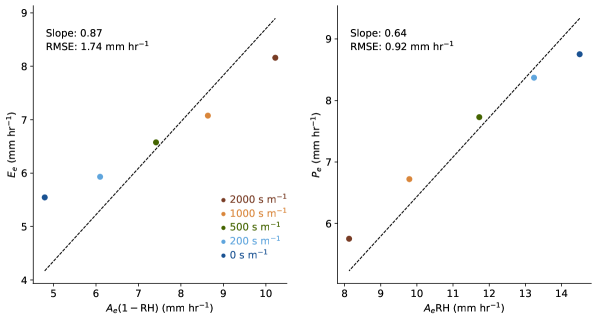
Fractional changes in condensation may, in turn, be decomposed into thermodynamic and dynamic contributions by using Equation (3). In this paper, thermodynamic contributions to condensation refer to changes in , which is a function of and , and also to changes in , which is a function of near-surface and (Romps, 2017). Dynamic contributions to condensation refer to changes in . Changes in the upper bound are neglected because and are both small in the upper troposphere. The thermodynamic and dynamic contributions to may be written succinctly by using a mask with when and when :
| (5) |
where the subscript indicates that the integrand terms are averaged at and above the th percentile of .
For extreme variables, sampling error was quantified using a block bootstrapping method. First, the samples were split into blocks of size km x km x time snapshot. Next, the set of blocks were resampled times with replacement to give new datasets of the same size. Finally, the extreme statistics (averages above a percentile) for each variable were computed for each resampling. Drawing blocks, instead of individual gridpoints, accounts for the spatially-correlated nature of heavy precipitation: convection has a larger footprint than a km x km gridbox.
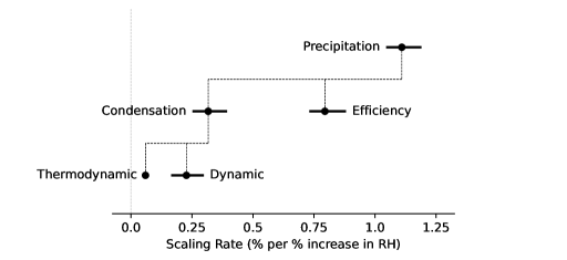
Figure 3 shows the resulting decomposition of the per scaling rate of with near-surface RH. Precipitation efficiency contributes the most to this scaling rate ( per ) although fractional changes in ( per ) are also substantial. Changes in are further decomposed into a dynamic contribution ( per ) and a small thermodynamic contribution ( per ). Thus, all three of the thermodynamic, dynamic and precipitation efficiency changes contribute positively to the increase in with increasing near-surface RH.
4 Understanding the thermodynamic contribution
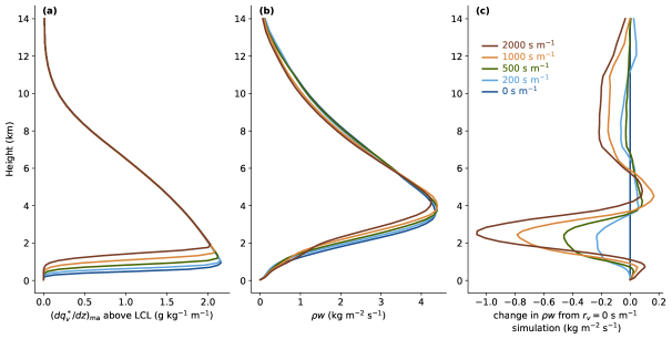
While small, the thermodynamic contribution of per in Fig. 3 is robust with a very small error bar. Free-tropospheric temperatures are relatively horizontally homogeneous and are constrained to not change in the horizontal mean as the surface dries, and thus the thermodynamic contribution must be explained by changes in the LCL rather than changes in free-tropospheric temperatures. To illustrate this, Fig. 4 plots the vertical structure of the factors composing the integrand in Equation (3). The moist-adiabatic moisture gradient is identical above 2 km across all values of (Fig. 4a): temperatures above this height are held fixed by the relaxation procedure described in Section 2.2, and so , which depends on temperature and pressure, stays approximately constant with increasing . However, since the condensation integral is not evaluated below and the LCL rises appreciably with increasing (as the near-surface air dries and warms), there is some negative thermodynamic contribution below km. This contribution is small because of relatively weak values of this close to the surface (Fig. 4b).
The thermodynamic contribution may be estimated by approximating that in the layer between LCLs, a) the cloud temperature follows a moist adiabat so that , and b) the upward mass flux is approximately constant with height so that where is a constant. Using the definition of the LCL as the height at which lifted near-surface air becomes saturated, the thermodynamic term in Equation (5) is approximately
| (6) |
where is the near-surface mixing ratio and and are the LCLs in the two climate states. Per Table 1, decreases from g kg-1 when s m-1 to g/kg when s m-1: a fractional change of per change in RH. However, with an average upward mass flux between the LCLs of kg m-2 s-1, mm hr-1 is roughly a quarter of the size of the condensation rate, mm hr-1.333, as defined in Equation (3), has units of kg m-2 s-1 but can be converted to mm/hr by dividing by the density of water, kg m-3, and multiplying by 1000 to convert from m to mm. Thus, Equation (6) predicts a thermodynamic contribution of per increase in RH, which is double the actual thermodynamic contribution. This difference can be explained by the fact that in the layer between LCLs, is about half as large as (not shown). Regardless, from Equation 6, we see that the thermodynamic contribution scales at a weaker rate than the near-surface mixing ratio because the water vapor flux at cloud base () is much smaller than the column-integrated condensation rate.
5 Understanding the dynamic contribution
The dynamic contribution to of per increase in RH is larger than the thermodynamic contribution. With increasing , Updrafts weaken the most in the lower troposphere, around to km (Figure 4b). Since this is above the LCL for each simulation and is large in the lower-troposphere, the dynamic contribution is more substantial than the thermodynamic contribution.
To understand what causes this dynamic contribution, we begin by inspecting buoyancy profiles, , averaged over columns exceeding the th-percentile value of . Buoyancy is defined in SAM as
| (7) |
where is the accelaration due to gravity, is the ratio of water and dry air gas constants minus one, is the mixing ratio for non-precipitating condensates, is the mixing ratio for falling precipitation, and quantities with the “env” subscript are horizontal- and time-mean “environmental” profiles. SAM uses horizontal-mean environmental profiles that are time-dependent. We simplify Equation (7) by neglecting time variations of the environmental profiles. We also neglect and in our calculation of buoyancy, even though can contribute substantial negative buoyancy within the cloud and in the boundary layer. We justify this simplification by assuming that in columns exceeding the th percentile of , this negative buoyancy primarily acts to form and strengthen downdrafts in the lower troposphere. Just as we considered only updrafts in Equation (3) and in calculating the dynamic contribution, here we consider only the buoyancy that generates those updrafts.
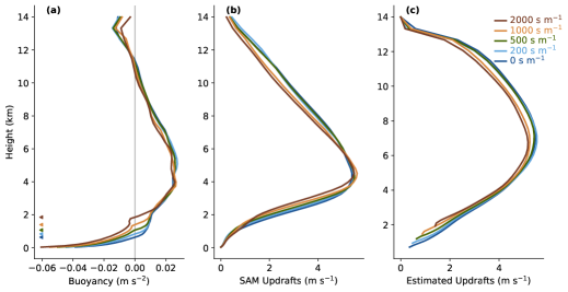
The changes in updrafts in the free troposphere can be broken into three distinct layers. Updrafts are weaker in drier simulations in the lower free troposphere (Fig. 5b), consistent with the loss of positive buoyancy. In a region between roughly and km, updrafts are roughly equal across all simulations. Above km, updrafts are once again weaker in drier simulations.
The buoyancy profiles in Fig. 5a suggest that the dynamic contribution is, like the thermodynamic contribution, mainly caused by changes in the LCL. To further investigate how buoyancy determines the updraft profiles, Fig. 5b compares profiles in high-percentile columns with given by solving
| (8) |
following the recommendation of Jeevanjee and Romps (2016). The parameter corresponds to the back-reaction from the environment on the parcel as it accelerates. The parameter represents the effect of different types of drag on a buoyant parcel besides the entrainment of momentum. Entrainment rates are inferred from values of moist static energy in columns exceeding the th percentile of , and different entrainment profiles were used for each simulation. For the other two parameters, the same constant values of and km-1 were used for all simulations. The methodology for determining the entrainment rate, , and is described in the Appendix.
| (s m-1) | |||||
|---|---|---|---|---|---|
| LCL (m) | |||||
| LFC (m) | |||||
| (m s-1) |
Equation (8) neglects mechanical lifting (e.g., from cold pools in the boundary layer), and so to estimate we integrate Equation (8) upwards from the level of free convection (LFC), defined as the height where in high-percentile columns (marked by triangles in Fig. 5a). Integrating Equation (8) below the LFC introduces negative buoyancy which would decrease our estimate of with height in the lower troposphere. Furthermore, the LFC largely follows the LCL: the LFC is only m above the LCL in the s m-1 simulation and m above the LCL in the s m-1 simulation (Table 2). Estimated profiles are initialized with an updraft velocity equal to at that simulation’s LFC. Values for the LCL, LFC, and in each simulation are reported in Table 2.
Updraft profiles calculated from Equation (8) capture the decreasing updraft velocities in the lower troposphere as increases (Fig. 5c). The value of does increase with increasing , but Fig. 5c shows that this is overcome by the loss of buoyancy as the LCL rises, such that decreases in the lower troposphere. The updrafts retain a memory of the loss of buoyancy from the rising LCL over a depth of no more than km, and as a result differences between estimated gradually shrink and are smallest around km (Fig. 5b). Above this height, a small decrease in with drier simulations causes profiles to diverge from one another again. This pattern mirrors the three-layer structure observed in , although profiles estimated using Equation (8) are more top-heavy than found in high-percentile columns. This may be related to using constant values of and with height, whereas in reality these parameters may change due to e.g., a change in a buoyant parcel’s aspect ratio (Jeevanjee and Romps, 2016). This may also be related to assumptions in the entrainment rate, as discussed in the Appendix.
Using estimated from Equation (8) in place of (except between the LCL and LFC) yields a dynamic contribution to changes in precipitation extremes of per change in RH, which is, surprisingly, identical to the actual dynamic contribution. If we repeat the plume calculation but only allow the LFC to change (holding the buoyancy profile and at its s m-1 value), the dynamic contribution is per demonstrating that the loss of positive buoyancy from the rising LCL is more than enough to explain the dynamical contribution. Increases in , which may be related to stronger turbulent eddies in a deeper boundary layer with a larger surface sensible heat flux, somewhat offset this loss of positive buoyancy.
6 Understanding changes in precipitation efficiency
6.1 Diagnosing contributions to precipitation efficiency
Precipitation efficiency is nearly three times as sensitive to near-surface RH as the condensation rate (Fig. 3). To understand what sets the precipitation efficiency, we take a similar approach to recent studies (Lutsko and Cronin, 2018; Da Silva et al., 2021) that have estimated as the product of two efficiencies that respectively describe conversion of cloud condensates to precipitation () and the extent to which precipitation reaches the surface without re-evaporating ():
| (9) |
The “conversion efficiency” compares the vertically integrated rate that precipitation is generated in the cloud, , to the vertically integrated rate of condensation, . In SAM’s one-moment microphysics scheme (Khairoutdinov and Randall, 2003), two processes generate precipitation. The first process, autoconversion, activates when the mixing ratio of non-precipitating condensates exceeds a Kessler threshold , and takes the form444SAM defines different coefficients for different condensate phases (liquid and ice) and for different precipitation types (rain, snow, and graupel). By the phrase “takes the form,” we mean that SAM calculates many similar terms with and partitioned by phase and type, using the appropriate coefficients in each case, that are then summed together.
| (10) |
The second process, collection of condensates by falling precipitation, takes the form
| (11) |
where is the mixing ratio for precipitating water and is an exponent unique to the precipitation type. We directly saved SAM’s microphysics tendencies from Equations (10) and (11), and used those tendencies to calculate :
| (12) |
A similar approach was taken for the “sedimentation efficiency” , where measures the proportion of the generated precipitation that re-evaporates in the column at a rate and thus doesn’t contribute to the surface precipitation rate . In SAM’s one-moment microphysics scheme, re-evaporation only occurs in locations where and takes the form
| (13) |
Note that in Equation (13) is evaluated at a given height (whereas elsewhere in this paper RH refers specifically to the near-surface value).
We directly saved SAM’s microphysics calculation of Equation (13) and used that value to calculate :
| (14) |
The relation is exact if all precipitation generated either evaporates or reaches the surface (i.e., if ). However, this is only the case if we average the different terms horizontally and over a sufficiently long time (as done by Lutsko and Cronin (2018)) because (a) precipitation can be transported or detrained horizontally prior to reaching the surface and (b) condensation, conversion to precipitation, evaporation, and precipitation reaching the surface can all occur at different times in a given convective lifecycle. The issue of non-locality in time is exacerbated by the use of instantaneous snapshots to calculate and , since that involves no time averaging at all.
To mitigate the effects of non-locality in time, in this section we use -hourly averaged output (instead of instantaneous snapshots) to calculate , , , and . We calculate as an average above the th percentile of , as done in Da Silva et al. (2021). , however, is calculated in columns that exceed the th percentile of under the assumption that re-evaporation occurs just before precipitation reaches the surface. Figure 6a shows the residual is about to mm hr-1 across the full range of simulations, which is roughly a quarter the size of .
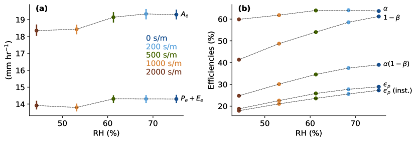
6.2 Re-evaporation explains efficiency increase with increasing relative humidity
Precipitation efficiency based on -hourly averaged values of and closely matches the instantaneous precipitation efficiency, with both spanning about to across the full range of simulations (Fig. 6b). Figure 6b also shows the -hourly averaged conversion efficiency , and the sedimentation efficiency as a function of RH. The sedimentation efficiency increases steadily with RH while the conversion efficiency is relatively constant with RH. The combination is close to but consistently larger than . Much like the residual , the ratio between and is an indirect measure of processes not accounted for in Equation (9), such as horizontal detrainment of falling precipitation.
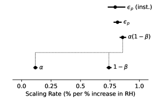
With the use of Equation (9), fractional changes in may be decomposed into fractional changes in and ,
| (15) |
and this decomposition is plotted in Fig. 7. Changes in both the conversion and sedimentation efficiencies contribute, but changes in the sedimentation efficiency are much larger. The estimate increases with RH at a rate of per , close to per fractional increase in -hourly averaged , implying our decomposition is reasonably accurate.
We focus on the sedimentation efficiency since its contribution is much larger. Fractional changes in sedimentation efficiency can, in turn, be attributed to fractional changes in and :
| (16) |
where we have substituted in and . Equation (16) is approximate because both of these substitutions assume that exactly. Equation (16) states that the fractional change in is set by a balance between fractional changes in the amount of precipitation generated, , and the amount of precipitation that re-evaporates while falling, .
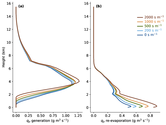
The contributions to and at different vertical levels across simulations with various are shown in Fig. 8. As increases, the contribution to increases in the mid-troposphere but decreases in the lower free troposphere, while the contribution to increases throughout the boundary layer and lower free troposphere. Increases in with are a direct result of a deeper and drier boundary layer at high , since re-evaporation is proportional to per Equation (13) and is only non-zero outside of the cloud. When integrated vertically, these profiles yield an that decreases relatively slowly with increasing and an that increases with increasing . Thus changes in both and contribute to a decrease in as is increased.
Finally, we derive some scalings that show how sedimentation efficiency might be related to changes in near-surface RH. Given that evaporation in the subcloud layer will roughly scale with the amount of precipitation generated at higher vertical levels, and given the dependence of Equation (13) on , we approximate such that . Substituting this into Equation (16) gives that
| (17) |
which directly relates changes in the sedimentation efficiency to changes in RH. The approximation underestimates changes in (Fig. 9a), likely because it neglects the vertical variations of and the precipitation generation rate, as well as the detailed dependence of evaporation rate on terminal velocity and other microphysical factors.
An alternate but related scaling is .555In the special case that these two scalings have slopes of , i.e. that and , these two scalings are identical so long as . This scaling is simple and intuitive: states that precipitation at the surface a) is directly proportional to the amount of condensation converted into precipitation aloft, and b) that drier boundary layers reduce surface precipitation (implicitly by increasing re-evaporation). Figure 9 shows that is a better empirical fit than is to . Using we have the simple prediction that and
| (18) |
i.e., that scales with RH at a rate of per . Equation (18) is a modest overestimate of the actual scaling rate of sedimentation efficiency at per .
Overall, these simple scalings are approximate but help by showing how the sedimentation efficiency and precipitation rate can be related to near-surface RH.
7 Conclusions
Using a CRM run to states of RCE, we found that convective precipitation extremes are sensitive to near-surface RH: between our wettest and driest simulations, instantaneous precipitation extremes fractionally decrease by for every fractional decrease in near-surface RH. When normalized by absolute rather than fractional changes in RH, precipitation extremes are more sensitive to near-surface RH over drier surfaces. Specifically, scaling rates range from per pt between our two wettest simulations () to per pt between our two driest simulations ().
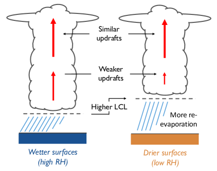
Three distinct physical mechanisms, all associated with changes in near-surface RH, explain these scaling rates. First, a weak thermodynamic contribution is found in direct response to changes in the LCL, which follow from changes in near-surface RH (Section 4). Second, a dynamic contribution also depends on changes in the LCL because positive buoyancy is only realized above the cloud base (Section 5). Third, re-evaporation is proportional to a factor of , and so precipitation efficiency is much lower in simulations with deeper, drier boundary layers (Section 6). These effects are illustrated schematically in Fig. 10.
The above three physical mechanisms– involving changes in the LCL and changes in re-evaporation– are all distinct from mechanisms that have been used to explain the Clausius-Clapeyron scaling of precipitation extremes with warming. Clausius-Clapeyron scaling has been explained by relating precipitation extremes to near-surface temperatures via specific humidity, either through moisture convergence arguments (Trenberth, 1999; Allen and Ingram, 2002) or through simplifications of the condensation integral (O’Gorman and Schneider, 2009; Abbott et al., 2020). All of these explanations rely on an assumption of constant RH, but the scaling rates calculated in this study suggest that a decrease in RH of over a dry surface, or a decrease in RH of over a moist surface, is sufficient to offset the effect of 1 K of warming and a Clausius-Clapeyron scaling rate of K-1. Note our simulations already include the effect of surface warming as the surface dries when the free-tropospheric temperature is held constant (Fig. 1b). This warming, explained by the top-down model of the land-ocean warming contrast (Joshi et al., 2008; Byrne and O’Gorman, 2013), would be in addition to the 1 K of surface warming mentioned above that warms the free troposphere (and thus increases in Equation (3)).
Overall, despite many differences including considering instantaneous or 3-hourly precipitation rather than daily precipitation, our study provides support, based on convection-resolving simulations, for the conclusion of Williams and O’Gorman (2022) that decreases in relative humidity are important for changes in summertime midlatitude precipitation extremes over land. Williams and O’Gorman (2022) considered whether such a correlation may be related to the dependence of convective inhibition (CIN)– negative buoyancy in the lower troposphere– on RH, since Chen et al. (2020) found that CIN increased as RH decreased and the LCL and LFC rose. While Williams and O’Gorman (2022) did find a correlation between changes in seasonal-mean CIN and the dynamical contribution to changes in precipitation extremes, the correlation was much weaker for CIN on the day of the precipitation event, casting doubt on the causality. Our results suggest an alternative cause: that updrafts weaken because of a decrease in positive buoyancy rather than an increase in negative buoyancy. However, CIN plays less of a role for convection in RCE compared to convection over midlatitude land (e.g., Markowski and Richardson, 2010; Agard and Emanuel, 2017; Emanuel, 2023), and thus further investigation of the midlatitude land case is warranted.
We find that the dynamic contribution is smaller than the contribution from changes in precipitation efficiency, whereas Williams and O’Gorman (2022) found a substantial dynamical contribution and did not consider a contribution from changes in precipitation efficiency. However, re-evaporation within downdrafts may be indirectly represented in the dynamical contribution of Williams and O’Gorman (2022) because they evaluate the condensation integral with a lower bound of instead of and allow for . Their definition is the same as the condensation integral introduced by O’Gorman and Schneider (2009), but in this paper we use a different definition (Equation (3)) that measures only condensation driven by updrafts above the cloud base. As a result of our alternate definition, we were able to separately diagnose changes in the precipitation efficiency resulting from changes in re-evaporation (Section 6).
Our finding that decreases in RH weaken precipitation extremes seems to be at odds with a scaling analysis of observed variability by Lenderink et al. (2024) which found that precipitation extremes were stronger at lower RH for a given dewpoint temperature. Part of this result of Lenderink et al. (2024) is a statistical effect related to conditioning on wet hours only, but the result still persisted more weakly when all hours were considered. One possible reason for the discrepancy is that our simulations focus on changes in horizontal- and time-mean near-surface RH in a state of RCE whereas Lenderink et al. (2024) analyze weather variability in hourly near-surface RH. Such weather variability could allow environments with lower near-surface RH to correspond to greater convective instability or greater convective organization.
Skinner et al. (2017) found in GCM simulations that stomatal closure causes widespread decreases in RH over land and decreases in mean precipitation in northern midlatitudes in summer, but that stomatal closure could actually increase mean and extreme precipitation in some regions of the deep tropics over land. These contrasting precipitation sensitivities in different regions suggest that large-scale dynamics may play an important role in the response of precipitation extremes to near-surface RH. Our results could be extended to include the influence of changing large-scale vertical velocity in future work by using a parameterization of the large-scale dynamics such as the weak-temperature gradient approximation (Sobel and Bretherton, 2000; Raymond and Zeng, 2005).
In conclusion, we have shown how changes in near-surface RH affect the intensity of precipitation in the simplest statistical-equilibrium case of RCE. In future work, we plan to address the scaling of precipitation extremes across a wide range of different temperatures and humidities in a similar RCE setting. In addition to incorporating the role of large-scale circulation as discussed earlier, future work should also include simulations with a diurnal cycle, since convection over land is heavily influenced by the diurnal cycle. It would also be interesting to consider the case of organized convection which may respond differently to changes in surface RH.
Determining parameters in the plume vertical velocity equation
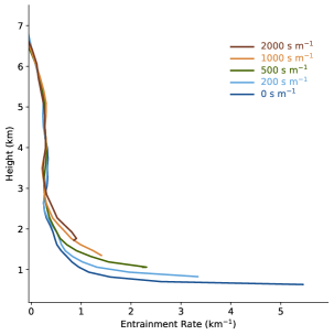
The entrainment rates used in Section (5) were estimated by assuming that within extreme columns (averaged above the 99.9th percentile), saturation frozen moist static energy (MSE) is mixed with the environmental frozen MSE following a bulk entraining plume:
| (19) |
Frozen MSE is defined following SAM thermodynamics as
| (20) |
where is the specific heat at constant pressure, is gravity, and are the latent heats of vaporization and fusion, respectively, and is a partition function that SAM uses to distinguish between liquid and ice condensates (Khairoutdinov and Randall, 2003). is defined by replacing with in Equation (20). Based on this assumption, can be computed by inverting Equation (19):
| (21) |
Figure 11 plots the entrainment rates estimated from high-percentile . Above km, increases with height in high-percentile columns, which implies an unphysical . Increasing with height cannot be explained by a single entraining plume, but it can be explained by a spectrum of plumes with different entrainment rates (Zhou and Xie, 2019). It is plausible that a spectral approach may improve upon the estimated from Equation (8), which is too strong in the region where increases with height. However, given our interest specifically in the lower free troposphere, we use a single bulk plume for its simplicity and set km-1 where it would otherwise be negative. This is a reasonable simplification to the extent that in the upper troposphere.
Constant values for the parameters and were fit to the s m-1 simulation and were determined in two steps. First, was calculated using values for , , and at the height where achieves its maximum value, . At this height, the left hand side of Equation (8) vanishes, so that
| (22) |
To determine , we solved Equation (8) for a range of values between and , using this value of . We chose the value of that matched the maximum value of to the high-percentile column’s maximum . When choosing , we did not require that achieved its maximum value at the same height as in the high-percentile column.
Acknowledgements.
We thank Tim Cronin for helpful discussions, particularly regarding the analysis of precipitation efficiency. This research is part of the MIT Climate Grand Challenge on Weather and Climate Extremes. Support was provided by Schmidt Sciences, LLC. \datastatementSAM is available at: http://rossby.msrc.sunysb.edu/SAM.html. Our code and data, including modifications to SAM, scripts to generate our simulations, post-processed data, and scripts and Jupyter notebooks to analyze data are available at: https://doi.org/10.5281/zenodo.14416632References
- Abbott et al. (2020) Abbott, T. H., T. W. Cronin, and T. Beucler, 2020: Convective dynamics and the response of precipitation extremes to warming in radiative–convective equilibrium. Journal of the Atmospheric Sciences, 77 (5), 1637–1660.
- Abramian et al. (2023) Abramian, S., C. Muller, and C. Risi, 2023: Extreme precipitation in tropical squall lines. Journal of Advances in Modeling Earth Systems, 15 (10), e2022MS003 477.
- Agard and Emanuel (2017) Agard, V., and K. Emanuel, 2017: Clausius–Clapeyron scaling of peak cape in continental convective storm environments. Journal of the Atmospheric Sciences, 74 (9), 3043–3054.
- Allen and Ingram (2002) Allen, M. R., and W. J. Ingram, 2002: Constraints on future changes in climate and the hydrologic cycle. Nature, 419 (6903), 224–232.
- Ban et al. (2015) Ban, N., J. Schmidli, and C. Schär, 2015: Heavy precipitation in a changing climate: Does short-term summer precipitation increase faster? Geophysical Research Letters, 42 (4), 1165–1172.
- Barbero et al. (2018) Barbero, R., S. Westra, G. Lenderink, and H. Fowler, 2018: Temperature-extreme precipitation scaling: A two-way causality? International Journal of Climatology, 38, e1274–e1279.
- Berg et al. (2016) Berg, A., and Coauthors, 2016: Land-atmosphere feedbacks amplify aridity increase over land under global warming. Nature Climate Change, 6 (9), 869–874.
- Betts (2000) Betts, A. K., 2000: Idealized model for equilibrium boundary layer over land. Journal of Hydrometeorology, 1 (6), 507–523.
- Byrne and O’Gorman (2013) Byrne, M. P., and P. A. O’Gorman, 2013: Link between land-ocean warming contrast and surface relative humidities in simulations with coupled climate models. Geophysical Research Letters, 40 (19), 5223–5227.
- Byrne and O’Gorman (2016) Byrne, M. P., and P. A. O’Gorman, 2016: Understanding decreases in land relative humidity with global warming: Conceptual model and gcm simulations. Journal of Climate, 29 (24), 9045–9061.
- Byrne and O’Gorman (2018) Byrne, M. P., and P. A. O’Gorman, 2018: Trends in continental temperature and humidity directly linked to ocean warming. Proceedings of the National Academy of Sciences, 115 (19), 4863–4868.
- Byrne and O’Gorman (2013) Byrne, M. P., and P. A. O’Gorman, 2013: Land–ocean warming contrast over a wide range of climates: Convective quasi-equilibrium theory and idealized simulations. Journal of Climate, 26 (12), 4000–4016.
- Cao et al. (2010) Cao, L., G. Bala, K. Caldeira, R. Nemani, and G. Ban-Weiss, 2010: Importance of carbon dioxide physiological forcing to future climate change. Proceedings of the National Academy of Sciences, 107 (21), 9513–9518.
- Chen et al. (2020) Chen, J., A. Dai, Y. Zhang, and K. L. Rasmussen, 2020: Changes in convective available potential energy and convective inhibition under global warming. Journal of Climate, 33 (6), 2025–2050.
- Cronin (2014) Cronin, T. W., 2014: On the choice of average solar zenith angle. Journal of the Atmospheric Sciences, 71 (8), 2994–3003.
- Da Silva et al. (2021) Da Silva, N. A., C. Muller, S. Shamekh, and B. Fildier, 2021: Significant amplification of instantaneous extreme precipitation with convective self-aggregation. Journal of Advances in Modeling Earth Systems, 13 (11), e2021MS002 607.
- Emanuel (2023) Emanuel, K., 2023: On the physics of high cape, under review (manuscript recieved via personal communication).
- Fowler et al. (2021) Fowler, H. J., and Coauthors, 2021: Anthropogenic intensification of short-duration rainfall extremes. Nature Reviews Earth & Environment, 2 (2), 107–122.
- Hansen and Back (2015) Hansen, Z. R., and L. E. Back, 2015: Higher surface Bowen ratios ineffective at increasing updraft intensity. Geophysical Research Letters, 42 (23), 10–503.
- Jeevanjee and Romps (2016) Jeevanjee, N., and D. M. Romps, 2016: Effective buoyancy at the surface and aloft. Quarterly Journal of the Royal Meteorological Society, 142 (695), 811–820.
- Joshi et al. (2008) Joshi, M. M., J. M. Gregory, M. J. Webb, D. M. Sexton, and T. C. Johns, 2008: Mechanisms for the land/sea warming contrast exhibited by simulations of climate change. Climate dynamics, 30, 455–465.
- Khairoutdinov and Randall (2003) Khairoutdinov, M. F., and D. A. Randall, 2003: Cloud resolving modeling of the arm summer 1997 IOP: Model formulation, results, uncertainties, and sensitivities. Journal of the Atmospheric Sciences, 60 (4), 607–625.
- Kharin et al. (2013) Kharin, V. V., F. W. Zwiers, X. Zhang, and M. Wehner, 2013: Changes in temperature and precipitation extremes in the CMIP5 ensemble. Climatic change, 119, 345–357.
- Laguë et al. (2021) Laguë, M. M., M. Pietschnig, S. Ragen, T. A. Smith, and D. S. Battisti, 2021: Terrestrial evaporation and global climate: Lessons from northland, a planet with a hemispheric continent. Journal of Climate, 34 (6), 2253–2276.
- Laguë et al. (2023) Laguë, M. M., G. R. Quetin, S. Ragen, and W. R. Boos, 2023: Continental configuration controls the base-state water vapor greenhouse effect: lessons from half-land, half-water planets. Climate Dynamics, 1–22.
- Langhans et al. (2015) Langhans, W., K. Yeo, and D. M. Romps, 2015: Lagrangian investigation of the precipitation efficiency of convective clouds. Journal of the Atmospheric Sciences, 72 (3), 1045–1062.
- Lenderink et al. (2024) Lenderink, G., N. Ban, E. Brisson, S. Berthou, V. E. Cortés-Hernández, E. Kendon, H. Fowler, and H. de Vries, 2024: Are dependencies of extreme rainfall on humidity more reliable in convection-permitting climate models? Hydrology and Earth System Sciences Discussions, 2024, 1–31.
- Lenderink et al. (2021) Lenderink, G., H. de Vries, H. J. Fowler, R. Barbero, B. van Ulft, and E. van Meijgaard, 2021: Scaling and responses of extreme hourly precipitation in three climate experiments with a convection-permitting model. Philosophical Transactions of the Royal Society A, 379 (2195), 20190 544.
- Lenderink et al. (2011) Lenderink, G., H. Mok, T. Lee, and G. Van Oldenborgh, 2011: Scaling and trends of hourly precipitation extremes in two different climate zones–hong kong and the netherlands. Hydrology and Earth System Sciences, 15 (9), 3033–3041.
- Lenderink and van Meijgaard (2010) Lenderink, G., and E. van Meijgaard, 2010: Linking increases in hourly precipitation extremes to atmospheric temperature and moisture changes. Environmental Research Letters, 5 (2), 025 208.
- Lepore et al. (2015) Lepore, C., D. Veneziano, and A. Molini, 2015: Temperature and cape dependence of rainfall extremes in the eastern united states. Geophysical Research Letters, 42 (1), 74–83.
- Lutsko and Cronin (2018) Lutsko, N. J., and T. W. Cronin, 2018: Increase in precipitation efficiency with surface warming in radiative-convective equilibrium. Journal of Advances in Modeling Earth Systems, 10 (11), 2992–3010.
- Markowski and Richardson (2010) Markowski, P., and Y. Richardson, 2010: Mesoscale meteorology in midlatitudes. John Wiley & Sons.
- Muller (2013) Muller, C., 2013: Impact of convective organization on the response of tropical precipitation extremes to warming. Journal of climate, 26 (14), 5028–5043.
- Muller et al. (2011) Muller, C. J., P. A. O’Gorman, and L. E. Back, 2011: Intensification of precipitation extremes with warming in a cloud-resolving model. Journal of Climate, 24 (11), 2784–2800.
- O’Gorman (2015) O’Gorman, P. A., 2015: Precipitation extremes under climate change. Current climate change reports, 1, 49–59.
- O’Gorman and Schneider (2009) O’Gorman, P. A., and T. Schneider, 2009: The physical basis for increases in precipitation extremes in simulations of 21st-century climate change. Proceedings of the National Academy of Sciences, 106 (35), 14 773–14 777.
- Pfahl et al. (2017) Pfahl, S., P. A. O’Gorman, and E. M. Fischer, 2017: Understanding the regional pattern of projected future changes in extreme precipitation. Nature Climate Change, 7 (6), 423–427.
- Prein et al. (2017) Prein, A. F., R. M. Rasmussen, K. Ikeda, C. Liu, M. P. Clark, and G. J. Holland, 2017: The future intensification of hourly precipitation extremes. Nature climate change, 7 (1), 48–52.
- Raymond and Zeng (2005) Raymond, D. J., and X. Zeng, 2005: Modelling tropical atmospheric convection in the context of the weak temperature gradient approximation. Quarterly Journal of the Royal Meteorological Society: A journal of the atmospheric sciences, applied meteorology and physical oceanography, 131 (608), 1301–1320.
- Romps (2011) Romps, D. M., 2011: Response of tropical precipitation to global warming. Journal of the Atmospheric Sciences, 68 (1), 123–138.
- Romps (2017) Romps, D. M., 2017: Exact expression for the lifting condensation level. Journal of the Atmospheric Sciences, 74 (12), 3891–3900.
- Sarbeng (2023) Sarbeng, E., 2023: Intense tropical thunderstorms in a future warmer climate. Ph.D. thesis, Monash University.
- Simmons et al. (2010) Simmons, A., K. Willett, P. Jones, P. Thorne, and D. Dee, 2010: Low-frequency variations in surface atmospheric humidity, temperature, and precipitation: Inferences from reanalyses and monthly gridded observational data sets. Journal of Geophysical Research: Atmospheres, 115 (D1).
- Simpson et al. (2024) Simpson, I. R., K. A. McKinnon, D. Kennedy, D. M. Lawrence, F. Lehner, and R. Seager, 2024: Observed humidity trends in dry regions contradict climate models. Proceedings of the National Academy of Sciences, 121 (1), e2302480 120.
- Singh and O’Gorman (2014) Singh, M. S., and P. A. O’Gorman, 2014: Influence of microphysics on the scaling of precipitation extremes with temperature. Geophysical Research Letters, 41 (16), 6037–6044.
- Skinner et al. (2017) Skinner, C. B., C. J. Poulsen, R. Chadwick, N. S. Diffenbaugh, and R. P. Fiorella, 2017: The role of plant CO2 physiological forcing in shaping future daily-scale precipitation. Journal of Climate, 30 (7), 2319–2340.
- Sobel and Bretherton (2000) Sobel, A. H., and C. S. Bretherton, 2000: Modeling tropical precipitation in a single column. Journal of climate, 13 (24), 4378–4392.
- Taylor et al. (2012) Taylor, K. E., R. J. Stouffer, and G. A. Meehl, 2012: An overview of CMIP5 and the experiment design. Bulletin of the American meteorological Society, 93 (4), 485–498.
- Trenberth (1999) Trenberth, K. E., 1999: Conceptual framework for changes of extremes of the hydrological cycle with climate change. Climatic change, 42 (1), 327–339.
- Westra et al. (2013) Westra, S., L. V. Alexander, and F. W. Zwiers, 2013: Global increasing trends in annual maximum daily precipitation. Journal of Climate, 26 (11), 3904–3918.
- Williams and O’Gorman (2022) Williams, A. I., and P. A. O’Gorman, 2022: Summer-winter contrast in the response of precipitation extremes to climate change over northern hemisphere land. Geophysical Research Letters, 49 (10), e2021GL096 531.
- Zhou et al. (2023) Zhou, W., L. R. Leung, and J. Lu, 2023: The role of interactive soil moisture in land drying under anthropogenic warming. Geophysical Research Letters, 50 (19), e2023GL105 308.
- Zhou and Xie (2019) Zhou, W., and S.-P. Xie, 2019: A conceptual spectral plume model for understanding tropical temperature profile and convective updraft velocities. Journal of the Atmospheric Sciences, 76 (9), 2801–2814.
- Zipser et al. (2006) Zipser, E. J., D. J. Cecil, C. Liu, S. W. Nesbitt, and D. P. Yorty, 2006: Where are the most intense thunderstorms on earth? Bulletin of the American Meteorological Society, 87 (8), 1057–1072.