Interacting dark sector with quadratic coupling: theoretical and observational viability

Abstract

Models proposing a non-gravitational interaction between dark energy (DE) and dark matter (CDM) have been extensively studied as alternatives to the standard cosmological model. A common approach to describing the DE-CDM coupling assumes it to be linearly proportional to the dark energy density. In this work, we consider the model with interaction term $Q=3H\gamma{\rho_{x}^{2}}/{(\rho_{c}+\rho_{x})}$. We show that for positive values of $\gamma$ this model predicts a future violation of the Weak Energy Condition (WEC) for the dark matter component, and for a specific range of negative values of $\gamma$ the CDM energy density can be negative in the past. We perform a parameter selection analysis for this model using data from Type Ia supernovae, Cosmic Chronometers, Baryon Acoustic Oscillations, and CMB combined with the Hubble constant $H_{0}$ prior. Imposing a prior to ensure that the WEC is not violated, our model is consistent with $\Lambda$CDM in 2$\sigma$ C.L.. In reality, the WEC prior shifts the constraints towards smaller values of $H_{0}$, highlighting an increase in the tension on the Hubble parameter. However, it significantly improves the parameter constraints, with a preference for smaller values of $\sigma_{8}$, alleviating the $\sigma_{8}$ tension between the CMB results from Planck 2018 and the weak gravitational lensing observations from the KiDS-1000 cosmic shear survey. In the case without the WEC prior, our model seems to alleviate the $H_{0}$ tension, which is related to the positive value of the interaction parameter $\gamma$.

1 Introduction

In the face of the discovery of the accelerated expansion of the Universe from observations of Type Ia Supernovae (SNe Ia) [1, 2, 3], a new model of the Universe comes into effect, containing characteristics of negative pressure energy content, referred to in the literature as dark energy (DE) [4]. Despite the great observational success of the standard $\Lambda$CDM model, where CDM stands for cold dark matter, it presents some shortcomings, such as the cosmological constant problem, the cosmic coincidence, and the Hubble constant tension. Therefore several models or approaches are attempting to obtain a better description of the nature of dark energy, which could be theoretically associated with quantum vacuum states. However, the cosmological constant still stands as the simplest candidate to be the component of dark energy [5, 6, 7, 8, 9, 10, 11, 12, 13].

In this work, we focus on a class of interacting models commonly referred to in the literature as interacting dark energy models (IDEM), with particular attention to the model designated as IDEM 2 in Ref. [10]. These models depart from the standard assumption of dark matter (DM) and dark energy (DE) as independent components by introducing a non-gravitational interaction, resulting in an energy exchange between them. Such interacting models are primarily phenomenologically motivated, reflecting our limited understanding of the fundamental physics underlying a coupling term [10, 14, 15].

A common choice for a IDEM assume that the interaction term $Q$ is linearly proportional to the DE density, i.e., $Q=3\gamma H\rho_{x}$, where $H$ and $\gamma$ represent the Hubble and interaction parameters, respectively (see, e.g., Refs. [10, 16, 17, 18, 19]). However, as demonstrated in Ref. [14], this class of models can exhibit non-physical behavior for certain parameter ranges, specifically predicting negative pressureless matter densities, thereby violating the Weak Energy Condition (WEC). In this work, we consider a model in which the interaction term is given by $Q\propto\rho_{x}^{2}/\left(\rho_{c}+\rho_{x}\right),$ deviating from the conventional linear interaction forms. The quadratic dependence on $\rho_{x}$ introduces a richer dynamical evolution, reflecting a more complex interplay between DE and CDM. Nevertheless, similar to the linear case, we show that this model also presents non-physical behavior for specific parameter values, with implications for the Universe’s background evolution and the growth of cosmic structures [20, 21].

This paper is organized as follows: In Section 2, we introduce the background dynamics for the cosmological model in analysis. In Section 3, we present the linear perturbation theory for interacting perfect fluids, while in Section 4 we detail the observational data used, the methodology, and the statistical analysis involved. The statistical analysis is based on MontePython  and a suitable modified version of Cosmic Linear Anisotropy Solving System (CLASS)  codes. In Section 5, we discuss the main results obtained. Finally, we present our conclusions in Section 6.

2 Background Dynamics

Let’s consider the energy balance equations, without fixing the state equation parameter at $\omega_{x}=-1$, but leaving it as a constant parameter. Thus, the energy conservation law for baryons, CDM, and DE are given, respectively, by

$$\dot{\rho}_{b}+3H\rho_{b} =0\,,$$ (1)

$$\dot{\rho}_{c}+3H\rho_{c} =-Q\,,$$ (2)

$$\dot{\rho}_{x}+3H\rho_{x}\left(1+\omega_{x}\right) =Q\,,$$ (3)

where $\rho_{c}$, $\rho_{x}$, and $\rho_{b}$ are respectively the densities of CDM, DE, and conserved baryons. The term $\omega_{x}$ is the DE equation-of-state (EoS) parameter. In this work, we are interested in the energy exchange between DM and DE described by the IDEM 2 in Ref. [10], which is characterized by the interaction term given by

$$Q=3H\gamma\dfrac{\rho_{x}^{2}}{\rho_{c}+\rho_{x}},$$ (4)

where $H$ and $\gamma$ are respectively the Hubble factor and interaction parameter.

The background solution for the densities of dark matter and dark energy are derived from the resolutions of equations (2) and (3) and are expressed as follows:

$$\rho_{c} ={\frac{3H_{0}^{2}}{8\pi G}}\ a^{-\frac{3\left(\omega_{x}+\omega_{x}^{2}+\gamma\right)}{\omega_{x}+\gamma}}$$

$$\times\left[\frac{\Omega_{x0}\left(\omega_{x}+\gamma\right)+\left(\Omega_{c0}\omega_{x}-\Omega_{x0}\gamma\right)a^{3\omega_{x}}}{\left(\Omega_{c0}+\Omega_{x0}\right)\omega_{x}}\right]^{-\frac{\gamma}{\omega_{x+\gamma}}}$$

$$\times\left[\Omega_{\mathrm{c0}}a^{3\omega_{x}}+\Omega_{x0}\frac{\gamma}{\omega_{x}}\left(1-a^{3\omega_{x}}\right)\right]$$ (5)

and

$$\rho_{x} ={\frac{3H_{0}^{2}}{8\pi G}\Omega_{x0}}\ a^{-\frac{3\left(\omega_{x}+\omega_{x}^{2}+\gamma\right)}{\omega_{x}+\gamma}}$$

$$\times\left[\frac{\Omega_{x0}\left(\omega_{x}+\gamma\right)+\left(\Omega_{c0}\omega_{x}-\Omega_{x0}\gamma\right)a^{3\omega_{x}}}{\left(\Omega_{c0}+\Omega_{x0}\right)\omega_{x}}\right]^{-\frac{\gamma}{\omega_{x+\gamma}}}\,$$ (6)

where $\Omega_{x0}$ and $\Omega_{c0}$ are the current DE and DM density parameters. It is possible to express it in a unified way,

$$r\left(a\right)=r_{0}\,a^{3\omega_{x}}+\dfrac{\gamma}{\omega_{x}}\left(1-a^{3\omega_{x}}\right)\,,$$ (7)

where $r(a)$ is defined as the ratio between the dark matter density and the dark energy density, $r(a)\equiv\rho_{c}/\rho_{x}$. In this case, when $\omega_{x}<0$, and in the limit where the scale factor $a(t)$ tends to infinity, $r(a)$ approaches a constant value, which differs from the standard $\Lambda$CDM model that tends to zero. Figure 1 shows curves of $r(a)$ for different values of the interaction parameter $\gamma$, while Figure 2 shows the density parameter of the energy components, both with the EoS parameter fixed respectively at $\omega_{x}=-0.8$, $\omega_{x}=-1$, and $\omega_{x}=-1.2$.

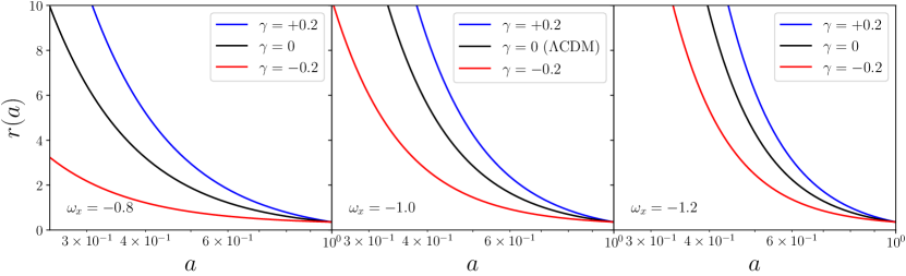
Figure 1: Ratio between the dark matter density and the dark energy density. Left panel: The black line represents the model with $\gamma=0$, the red lines have $\gamma=-0.2$, and the blue lines have $\gamma=+0.2$, with the EoS parameter fixed at $\omega_{x}=-0.8$. Central panel: The black line represents the model with $\gamma=0$ (non-interacting case, i.e., reduces to the $\Lambda$CDM model), the red lines have $\gamma=-0.2$, and the blue lines have $\gamma=+0.2$, with the EoS parameter fixed at $\omega_{x}=-1$. Right panel: The black line represents the model with $\gamma=0$, the red lines have $\gamma=-0.2$, and the blue lines have $\gamma=+0.2$, with the EoS parameter fixed at $\omega_{x}=-1.2$. In all panels, DE density parameter was fixed at $\Omega_{x0}=0.7$.

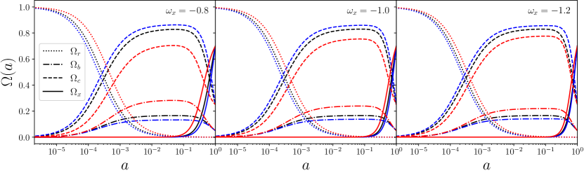
Figure 2: Evolution of the density parameters of the Universe’s components as a function of the scale factor. The EoS parameter was fixed respectively at $\omega_{x}=-0.8$ (left panel), $\omega_{x}=-1$ (central panel), and $\omega_{x}=-1.2$ (right panel). In all panels, the dotted line represents the radiation component, the dashed line represents dark matter, the dash-dotted line represents baryons, and the solid line represents the dark energy component. The black lines represent the model with $\gamma=0$, the red lines have $\gamma=-0.2$, and the blue lines have $\gamma=+0.2$.

We are interested in determining the regions where the densities $\rho_{x}$ and $\rho_{c}$ are greater than or equal to zero. Specifically, we want to find the allowed regions for the DE and DM densities during their cosmic evolution, as only these have physical significance. Given the definition $r(a)=\rho_{c}/\rho_{x}$, it is sufficient to evaluate only one of the pairs: $\rho_{x},\rho_{c}$ or $\rho_{x},r(a)$ or $\rho_{c},r(a)$. To ensure that the curves have values greater than or equal to zero, from the initial scale factor $a=0$ to $a\rightarrow\infty$, it is suitable to introduce a variable transformation of the type:

$$y=\frac{2}{\pi}\arctan(\bar{y}),$$ (8)

where $\bar{y}$ can be: $\rho_{c}$, $\rho_{x}$, $r$, or $a$. The x-axis, used for the scale factor, assumes the finite interval $x=[0,1]$, while y, being used for $\rho_{x}$, or $r$, assumes the finite interval $y=[-1,1]$.

To ensure that equation (2) satisfies $\rho_{x}\geq 0$, in Figure 3, was plotted $({2}/{\pi})\arctan(\rho_{x})$ versus $({2}/{\pi})\arctan(a)$ from a computation with 30000 of generated curves with the parameters $\omega_{x},~\gamma,~\Omega_{m0}$, and $h$ (where $h$ is $H/100$ km$/$s$/$Mpc) randomly varying between the intervals of $\omega_{x}=[-2,2]$, $\gamma=[-2,2]$, $\Omega_{m0}=[-1,1]$, and $h=[0.5,1]$, respectively.

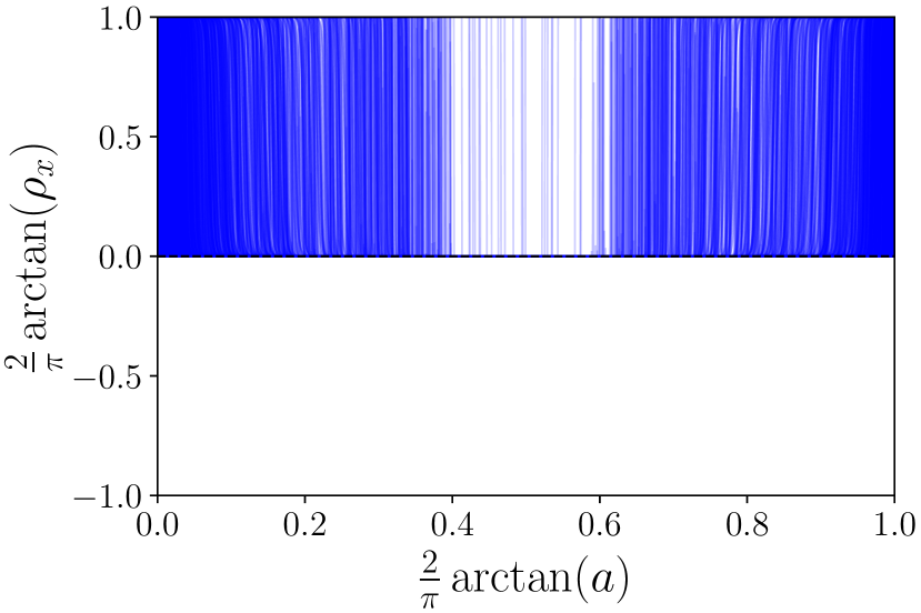
Figure 3: Computation with 30000 of curves of $\rho_{x}(a)$. The blue lines represent curves with values $\rho_{x}(a)\geq 0$. There were no curves for $\rho_{x}(a)<0$. The graph represents the largest possible scale for $\rho_{x}$ and $a$ ($\rho_{x}=[-\infty,\infty]$, $a=[0,\infty]$), with the parameters $\omega_{x},~\gamma,~\Omega_{m0}$, and $h$ randomly varying between the intervals of $\omega_{x}=[-2,2]$, $\gamma=[-2,2]$, $\Omega_{m0}=[-1,1]$, and $h=[0.5,1]$, respectively.

Meanwhile, Figure 4 shows the plot of $({2}/{\pi})\arctan(r)$ versus $({2}/{\pi})\arctan(a)$, built with the generation of 5000 curves, with the same random choice of the parameters $\omega_{x},~\gamma,~\Omega_{m0}$. In this figure, the dark matter density can assume negative values ($\rho_{c}<0$) for certain time intervals (in the past or in the future), thereby violating the WEC.

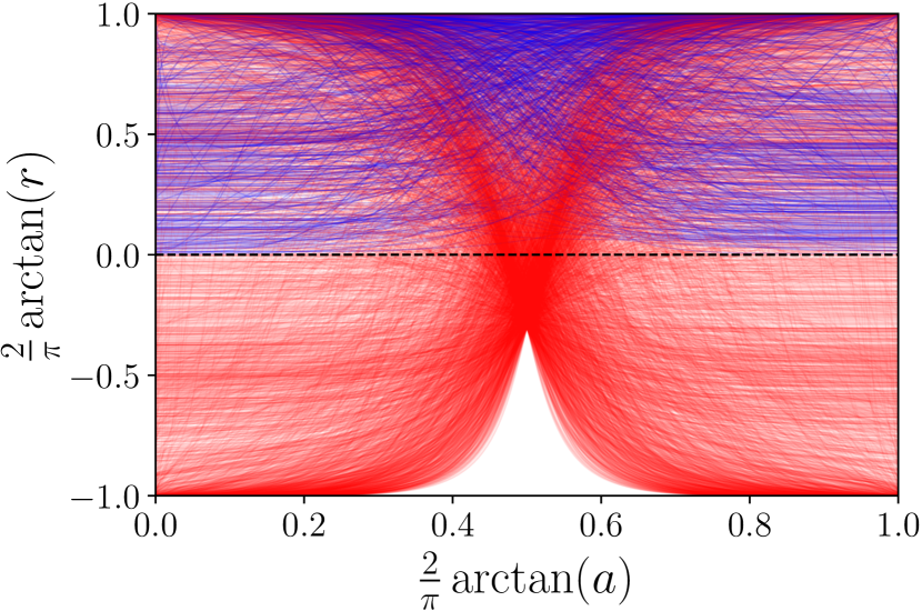
Figure 4: Computation with 5000 of curves of $r(a)$. The blue lines represent curves with values $r(a)\geq 0$, and the red lines represent curves with values that, at some point, have $r<0$. The graph represents the largest possible scale for $r$ and $a$ ($r=[-\infty,\infty]$, $a=[0,\infty]$), with the parameters $\omega_{x},~\gamma$, and $~\Omega_{m0}$ randomly varying between the intervals of $\omega_{x}=[-2,2]$, $\gamma=[-2,2]$, and $\Omega_{m0}=[-1,1]$, respectively.

From equation (2), it is possible to assess the conditions leading to the WEC violation. Thus, we can divide the analysis into two distinct periods: the past and the future, so that it can be observed that the energy density of matter assumes negative values at

$$a=\left[\frac{-\gamma\,\Omega_{x0}}{\omega_{x}\Omega_{c0}-\gamma\Omega_{x0}}\right]^{\frac{1}{3\,\omega_{x}}}.$$ (9)

Assuming that the value of the equation of state parameter is $\omega_{x}<0$, we straightly obtain the solution conditions for the equation (9) in the intervals $0<a<1$ (in the past) and $a>1$ (in the future). To prevent the dark matter energy density from becoming negative in the early moments of the universe, the interaction parameter must satisfy the following condition

$$\gamma>-\left|\omega_{x}\right|\frac{\Omega_{c0}}{\Omega_{x0}}.$$ (10)

However, it is likely that the density of dark matter, $\rho_{c}$, will be negative in the future, unless,

$$\gamma\leq 0,$$ (11)

that is independent of the value $\omega_{x}$. The equations (10) and (11) define the range in which the model is physically well-defined, regardless of the timescale. In Figure 5, the scale factor is depicted for the WEC violation as a function of the interaction parameter $\gamma$.

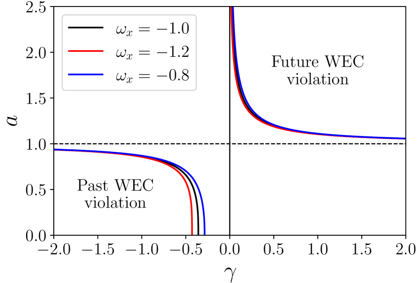
Figure 5: Plot of the scale factor $a$ that violates the WEC as a function of the interaction parameter $\gamma$. On the top right is shown the WEC violation in the future, while on the bottom left is shown the WEC violation in the past. The black line corresponds to $\omega_{x}=-1$, while the blue line corresponds to $\omega_{x}=-0.8$, and the red line corresponds to $\omega_{x}=-1.2$. Here, the dark energy density parameter was fixed at $\Omega_{x0}=0.7$.

Let’s consider, for example, $\omega_{x}=-1$, $\Omega_{x0}=0.7$ and $\gamma=0.2$ $\rho_{c}$ becomes negative with scale factor $a\approx 1.4$, where the critical density is $\rho_{cr0}=\frac{3H_{0}^{2}}{8\pi G}=1.87798\times 10^{-26}h^{2}\frac{\mathrm{kg}}{\mathrm{m}^{3}}$, with $h=0.7324$ [22]. Figure 6 shows how the universe evolves with the Hubble function, DE, and matter densities as a function of the scale factor.

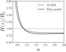
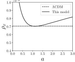
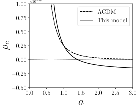
Figure 6: Background solutions of this model and the $\Lambda$CDM model as a function of the scale factor $a$. Left panel: Shows the Hubble function $H(z)/H_{0}$. Central panel: Dark energy density. Right panel: Dark matter density. In all panels, the solid line corresponds to the model, with $\omega_{x}=-1$, $\Omega_{x0}=0.7$, $\gamma=0.2$ and $h=0.7324$, and the dashed lines correspond to the $\Lambda$CDM model, with the same values of $\Omega_{x0}$ and $h$.

3 Perturbations

The description of the dark sector interaction for an interacting model, assuming a phenomenological nature, can be given through a covariant derivative of the energy-momentum tensor, where the equations for conserved baryons, DM and DE are

$$T_{b;\,\nu}^{\mu\nu}=0,$$ (12)

$$T_{c;\,\nu}^{\mu\nu}=Q^{\mu},$$ (13)

and

$$T_{x\,;\nu}^{\mu\nu}=-Q^{\mu}.$$ (14)

The term $Q^{\mu}$ is a four-vector that acts as a source for the energy-momentum tensor; the terms $T_{c}^{\mu\nu}$ and $T_{x}^{\mu\nu}$ are the energy-momentum tensors for dark matter and dark energy, respectively. In a perfect fluid, the spatial components for a covariant derivative of the energy-momentum tensor are zero. Consequently, in the background, the interaction term is given by a scalar function is $Q^{\mu}=(Q,\vec{0})$ in an unperturbed case (as seen in the previous section) [10, 15, 23, 24]. On the other hand, for a perturbed case and assuming scalar perturbations responsible for the formation of structures in the universe, the perturbed Friedmann-Lemaître-Robertson-Walker metric in a spatially flat universe considering the Newtonian gauge is given by [10, 25]

$$ds^{2}=a^{2}\left(\tau\right)\left[-\left(1+2\psi\right)d\tau^{2}+\left(1-2\phi\right)dx^{i}dx_{i}\right]$$ (15)

with the scalar degrees of freedom being $\psi$ and $\phi$, and using conformal time $\tau$ instead of cosmic time $t$.

In describing structure formation at the linear level, it is necessary to solve all the perturbation equations for each component of the universe. The temperature anisotropies of the CMB are derived by solving the Boltzmann equations for all components [25]. However, assuming that the baryon and radiation components are similar to those in the $\Lambda$CDM model, they interact with each other via Thomson scattering before recombination and are not directly connected to the dark sector [10, 25, 26].

Assuming a fluid dynamic description to represent the dark sector components, the perturbed fluid equations must incorporate the contribution of the interaction term. Thus, we can consider at the linear level the perturbative contribution divided into two components, one parallel and one orthogonal to the four-velocity,

$$Q^{\mu}=Qu^{\mu}+F^{\mu},$$ (16)

with $F^{\mu}u_{\mu}=0$. The first term on the right-hand side $Q$ is a scalar function with background components defined in equations (2) and (3). The perturbative contribution will be denoted by $\hat{Q}$ and has the form $\hat{Q}=\hat{\Theta}\gamma R+3H\gamma\hat{R}$, where $\hat{R}$ is model dependent and can be obtained by linearizing the expansion scalar $\Theta\equiv u^{\mu}_{\,;\mu}$, in Newtonian gauge it is expressed by

$$\hat{\Theta}=\dfrac{1}{a}\left(\theta_{tot}-\Theta\psi-3\phi^{\prime}\right),$$ (17)

where $\theta_{tot}$ is the divergence of the interacting fluid for the entire cosmic medium. The ideal fluid description of the dark sector components requires that the term $F^{\mu}$ has only a spatial perturbative contribution. Therefore, the total perturbative interaction term can be written as $\hat{Q}^{\mu}=a\left(Q\psi+\hat{Q},Q\hat{u}^{i}+F^{i}\right)$.

In considering the basic equations of the energy balance defined in Eqs. (13) and (14), taking into account a general interacting fluid with constant EoS $p=\omega\rho$ and perturbed four-velocity $\hat{u}^{\mu}=a^{-1}\left(-\psi,\partial^{i}v\right)$, where $v$ is its peculiar velocity. The conservation of energy and momentum in the Newtonian gauge is given by

$$\delta^{\prime} +3\mathcal{H}\left(c_{s}^{2}-\omega\right)\delta+9\mathcal{H}^{2}\left(1+\omega\right)\left(c_{s}^{2}-c_{a}^{2}\right)\dfrac{\theta}{k^{2}}$$

$$+\left(1+\omega\right)\left(\theta-3\phi^{\prime}\right)$$

$$=\dfrac{Qa}{\rho}\left[\dfrac{\hat{Q}}{Q}-\delta+\psi+3\mathcal{H}\left(c_{s}^{2}-c_{a}^{2}\right)\dfrac{\theta}{k^{2}}\right]\,,$$ (18)

$$\theta^{\prime}+\mathcal{H}\left(1-3c_{s}^{2}\right)\theta-\dfrac{k^{2}c_{s}^{2}}{1+\omega}\,\delta-k^{2}\psi$$

$$=\dfrac{a}{\rho\left(1+\omega\right)}\left[Q\theta_{tot}-k^{2}f-\left(1+c_{s}^{2}\right)Q\theta\right]\,.$$ (19)

In the above equations, primes denote derivatives with respect to conformal time, where $\mathcal{H}$ is the Hubble parameter in conformal time, defined as $\mathcal{H}=aH$. In equation (18) the density contrast $\delta\equiv\hat{\rho}/\rho$ is introduced, where $\hat{\rho}$ is the perturbative energy density and $\rho$ is the background energy density. In equation (19), the dynamical quantity of interest is the divergence of the interacting fluid $\theta\equiv i\,k^{a}\partial_{a}v$. Meanwhile, $\theta_{tot}$ denotes the same quantity, but for the entire cosmic medium, not limited to a single fluid. For scalar perturbations, it is useful to define the spatial contribution of the interaction term as $aF^{i}=\partial^{i}f$. Finally, $c_{a}^{2}$ and $c_{s}^{2}$ correspond to the adiabatic sound speed and the physical rest-frame sound speed for the fluid, respectively. Under the assumption of a constant EoS parameter, the adiabatic sound speed $c_{a}^{2}$ reduces to $\omega$.

Now, using the equations (18) and (19), we can write the perturbative equations for the dark sector components. For the CDM component, we have

$${\delta}_{c}^{\prime}+\theta{c}-3{\phi}^{\prime}=\dfrac{aQ}{\rho_{c}}\left(\delta_{c}-\dfrac{\hat{Q}}{Q}-\psi\right)\,,$$ (20)

$${\theta}_{c}^{\prime}+\mathcal{H}\theta_{c}-k^{2}\psi=\dfrac{aQ}{\rho_{c}}\left(\theta_{tot}-\theta_{c}\right)\,.$$ (21)

While for the DE component, it is expressed as

$${\delta}_{x}^{\prime} +\left(1+\omega_{x}\right)\left(\theta_{x}-3\phi^{\prime}\right)+3\mathcal{H}\left(c_{s}^{2}-\omega_{x}\right)\delta_{x}$$

$$=-\dfrac{aQ}{\rho_{x}}\left(\delta_{x}-\dfrac{\hat{Q}}{Q}\right)\,,$$ (22)

$$\theta_{x}^{\prime}+\mathcal{H}\left(1-3c_{s}^{2}\right)\theta_{x}-\frac{c_{s}^{2}k^{2}}{1+\omega_{x}}\delta_{x}-k^{2}\psi$$

$$= \frac{aQ}{(1+\omega_{x})\rho_{x}}\left[\theta_{tot}-(1+c_{s}^{2})\theta_{x}+(1+\omega_{x})\frac{\hat{Q}}{Q}\right].$$ (23)

To prevent instabilities, the physical speed of sound $c_{s}^{2}$ must not be negative in dynamical dark energy. Thus, we consider $c_{s}^{2}=1$, in agreement with several references [10, 26, 27, 28].

The perturbative interaction term is given by the linearization of the background interaction term (Eq. 4), which is expressed as [10]

$$\hat{Q}=Q\left(\dfrac{\hat{\Theta}}{\Theta}+\dfrac{\rho_{x}\delta_{x}+2\rho_{c}\delta_{x}-\rho_{c}\delta_{c}}{\rho_{c}+\rho_{x}}\right)\,.$$ (24)

In the background, the expansion scalar $\Theta$ simplifies to $\Theta=3H$ [10, 29].

4 Methodology

This section briefly describes the observational datasets and the statistical analysis methodology.

4.1 Observational Data

Here we will present the observational datasets.

• Type Ia Supernovae (SNe Ia): SNe Ia are considered standard candles in astronomy and have played a pivotal role in observing the Universe’s accelerated expansion [30, 1, 2, 3]. In general, the apparent magnitude and luminosity distance are related by $m=5\log\left(D_{L}\right)+25+M\,$, where $M$ is the absolute magnitude. $D_{L}(z)$ represents the luminosity distance expressed in units of Mpc. In this analysis, $1048$ measurements of apparent magnitudes from Type Ia supernovae were used, referred to as the Pantheon sample. This dataset covers the redshift range $0.01<z<2.3$ [31, 32].

• Current Value of the Hubble Expansion Rate ($H_{0}$): The Hubble expansion rate obtained by [22] provides the best estimate of $H_{0}=(73.24\pm 1.74)\,$km s^-1 Mpc^-1, from a set of observations containing more than 600 Cepheids, using both infrared and visible frequencies. This value is independent of the cosmological model.

• Cosmic Chronometers (CC): The Cosmic Chronometers are independent data from cosmological models, derived from measurements taken from ancient galaxies. There are $30$ measurements of $H(z)$ in the range $0.07<z<1.965$, as presented in Table 1 [33].

  Table 1: Measurements of $H(z)$, with their respective errors, containing the CC data.

  $z$	$H(z)$	$\sigma_{H(z)}$	References
  0.07	69.0	19.6	[34]
  0.09	69.0	12.0	[35]
  0.12	68.6	26.2	[34]
  0.17	83.0	8.0	[35]
  0.179	75.0	4.0	[36]
  0.199	75.0	5.0	[36]
  0.2	72.9	29.6	[34]
  0.27	77.0	14.0	[35]
  0.28	88.8	36.6	[34]
  0.352	83.0	14.0	[36]
  0.3802	83.0	13.5	[33]
  0.4	95.0	17.0	[35]
  0.4004	77.0	10.2	[33]
  0.4247	87.1	11.2	[33]
  0.4497	92.8	12.9	[33]
  0.4783	80.9	9.0	[33]
  0.48	97.0	62.0	[37]
  0.593	104.0	13.0	[36]
  0.68	92.0	8.0	[36]
  0.781	105.0	12.0	[36]
  0.875	125.0	17.0	[36]
  0.88	90.0	40.0	[37]
  0.9	117.0	23.0	[35]
  1.037	154.0	20.0	[36]
  1.3	168.0	17.0	[35]
  1.363	160.0	33.6	[38]
  1.43	177.0	18.0	[35]
  1.53	140.0	14.0	[35]
  1.75	202.0	40.0	[35]
  1.965	186.0	50.4	[38]

• Baryon Acoustic Oscillations (BAO): Baryon Acoustic Oscillations carry information from the pre-decoupling Universe. The baryon-photon fluid propagates with an acoustic velocity described as follows [39, 40]:

  $$c_{s}=\frac{c}{\sqrt{3(1+\mathrm{R})}},$$ (25)

  with $\mathrm{R}\equiv\frac{3\rho_{b}}{4\rho_{\gamma}}\propto\frac{\Omega_{b}}{1+z}$.

  After decoupling, photons begin to travel with a characteristic scale given by

  $$r_{s}(a_{\rm{drag}})\equiv\int_{0}^{a_{\rm drag}}\dfrac{c_{s}\left(a\right)}{Ha^{2}}\ da\,,$$ (26)

  where $c_{s}$ represents the speed of sound in the primordial plasma and $a_{\rm drag}$ is the scale factor at the drag time, referring to the moment in the early universe when photons and baryons (protons and neutrons) decoupled [41]. The isotropic BAO measurements are provided through the dimensionless ratio $D_{V}/r_{s}(a_{\rm{drag}})$, where $D_{V}$ is the geometric mean that combines the scales of the line-of-sight and transverse distances. $D_{V}$ is expressed by [42, 43]

  $$D_{V}(z)=\left[\left(1+z\right)^{2}D_{A}^{2}(z)\dfrac{cz}{H(z)}\right]^{1/3}\,,$$ (27)

  where $D_{A}(z)$ is the angular diameter distance. Here, the BAO data  is obtained from Refs. [44, 45, 46].

• CMB data (Planck): The data used here for CMB are measurements from Planck 2018, which include information on temperature, polarization, temperature polarization cross-correlation spectra, and lensing maps reconstruction, Planck (TT, TE, EE+lowE+lensing) [47]. In these analyses, the standard likelihood codes were considered: (i) COMANDER for the low-$l$ TT spectrum, with spectrum data ranging from $2\leq l<30$; (ii) SimAll for the low-$l$ EE spectrum, with spectrum data ranging from $2\leq l<30$; (iii) Plik TT, TE, EE for the TT, TE, and EE spectra, covering $30\leq l\lesssim 2500$ for TT and $30\leq l\lesssim 2000$ for TE and EE; (iv) lensing power spectrum reconstruction with $8\leq l\leq 400$. For more details on the likelihoods, see Refs. [47, 30].

4.2 Statistical analysis

Statistical analysis is performed using the MontePython code [48, 49], which utilizes the CLASS code [50, 49]. In the MontePython code, the Markov Chain Monte Carlo (MCMC) method [51, 52] is used to perform statistical analysis on the input data, comparing it with the theoretical predictions, that are provided by a suitably modified version of the CLASS code, to take into account the cosmology framework described in section 2. To use the $\Lambda$CDM and $\omega$CDM models, no modifications are necessary in the code. However, for other models, such as the interacting models, it is necessary to implement the background equations as well as the perturbed fluid equations with the linear perturbative contribution of the model in the code. For all chains, during the MCMC analysis in MontePython, it is required that the Gelman-Rubin convergence parameter satisfies the condition $\hat{R}-1<0.01$ [53, 54]. We utilized GetDist to analyze and plot the chains [55, 56]. It allows for creating contour plots, histograms, parameter correlations, among others, from datasets generated by codes such as MontePython. In this part, using the GetDist library, the samples where the parameter $\gamma$ does not satisfy the conditions of equations (10) and (11) were filtered. These equations establish specific limits for the value of $\gamma$ . Thus, only the samples that adhere to these restrictions are considered in the posterior analysis, specifically with the prior applied.

4.3 Combination of dataset

We investigate the impact of the physical or WEC prior, in the case of $\gamma\geq 0$, on the estimation of the cosmological parameters of the model under analysis. The unmodified CLASS code already automatically resolves past WEC violation. A Bayesian statistical analysis was conducted with and without the inclusion of such a prior, for five different datasets:

1. Background: Composed of SNe Ia, CC, and BAO data;

2. Background+$H_{0}$: Composed of SNe Ia, CC, BAO, and $H_{0}$ data;

3. Planck: Composed of the full CMB data from Planck, combined with Planck TTTEEE+lensing reconstruction;

4. Background+Planck: Composed of the combination of Planck+Background;

5. Background+Planck+$H_{0}$: Composed of the combination of Planck+Background, with $H_{0}$.

5 Results and discussion

When we do not include the Planck data in our analysis, we considered the following cosmological parameters: $\mathcal{P}$=$\{\omega_{c}$, $H_{0}$, $\gamma\}$ where $\omega_{c}$ is the cold dark matter density parameter, and the derived parameters: $\mathcal{P^{{}^{\prime}}}$=$\{\Omega_{m0}$, $\omega_{b}\}$ where $\omega_{b}$ and $\Omega_{m0}$ represent respectively the baryon and current matter density parameters. Otherwise when we include the data from Planck, the parameters are: $\mathcal{P}$=$\{100\theta{}_{s}$, $n_{s}$, $\ln$$(10^{10}A_{s})$, $\omega_{b}$, $\omega_{c}$, $\tau_{reio}$, $\gamma\}$ where $100\theta_{s}$, $n_{s}$, $\ln(10^{10}A_{s})$, and $\tau_{reio}$ are respectively the angular size of the sound horizon (scaled by 100), the scalar spectral index, the logarithm of the amplitude of the primordial scalar power spectrum, and the optical depth to reionization, and the derived parameters: $\mathcal{P^{{}^{\prime}}}$=$\{H_{0}$, $\Omega_{m0}$, $\sigma_{8}$, $S_{8}\}$, where $\sigma_{8}$ and $S_{8}$ are respectively the standard deviation of the density fluctuation in an 8 $h^{-1}$ Mpc radius sphere, and the structure growth parameters, with the equation of state parameter fixed at $\omega_{x}=-1$. The results of our analysis are presented in Tables 2 and 3, both with and without the WEC prior. For the background tests, the baryon density parameter was fixed at 0.05, while in the analyses that include CMB data, $\Omega_{b0}$ is a free parameter.

Table 2: Statistical analysis results at $1\sigma$ C.L., considering the analyses without and with the WEC prior, using the datasets: Background and Background+$H_{0}$.

Parameter	Background		Background+$H_{0}$
	No prior	WEC prior	No prior	WEC prior
$\gamma$	$-0.02^{+0.11}_{-0.11}$	$-0.088^{+0.071}_{-0.041}$	$-0.02^{+0.11}_{-0.11}$	$-0.095^{+0.084}_{-0.040}$
$\omega_{c}$	$0.124^{+0.017}_{-0.015}$	$0.132^{+0.010}_{-0.012}$	$0.124^{+0.017}_{-0.015}$	$0.134^{+0.010}_{-0.012}$
$H_{0}$	$69.1^{+1.7}_{-1.7}$	$68.6^{+1.3}_{-1.3}$	$69.1^{+1.7}_{-1.7}$	$68.3^{+1.4}_{-1.4}$
$\omega_{b}$	$0.0239^{+0.0012}_{-0.0012}$	$0.02352^{+0.00082}_{-0.00094}$	$0.0239^{+0.0012}_{-0.0012}$	$0.0236^{+0.00095}_{-0.00095}$
$\Omega_{m0}$	$0.310^{+0.040}_{-0.040}$	$0.334^{+0.018}_{-0.028}$	$0.310^{+0.041}_{-0.041}$	$0.338^{+0.022}_{-0.028}$

Table 3: Statistical analysis results at $1\sigma$ C.L., considering the analyses without and with the WEC prior, using the datasets: Planck, Planck+Background, and Planck+Background+$H_{0}$.

Parameter	Planck		Planck+Background		Planck+Background+$H_{0}$
	No prior	WEC prior	No prior	WEC prior	No prior	WEC prior
$\gamma$	$0.08^{+0.14}_{-0.11}$	$-0.078^{+0.070}_{-0.039}$	$0.062^{+0.070}_{-0.070}$	$-0.036^{+0.034}_{-0.020}$	$0.123^{+0.071}_{-0.071}$	$-0.031^{+0.029}_{-0.019}$
$100\theta{}_{s}$	$1.04191^{+0.00030}_{-0.00030}$	$1.04187^{+0.00030}_{-0.00030}$	$1.04197^{+0.00028}_{-0.00028}$	$1.04206^{+0.00028}_{-0.00024}$	$1.04200^{+0.00028}_{-0.00028}$	$1.04208^{+0.00027}_{-0.00027}$
$\ln 10^{10}A_{s}$	$3.045^{+0.015}_{-0.015}$	$3.044^{+0.014}_{-0.014}$	$3.046^{+0.012}_{-0.014}$	$3.048^{+0.011}_{-0.016}$	$3.047^{+0.014}_{-0.014}$	$3.049^{+0.012}_{-0.015}$
$n_{s}$	$0.9654^{+0.0041}_{-0.0041}$	$0.9647^{+0.0040}_{-0.0040}$	$0.9669^{+0.0037}_{-0.0037}$	$0.9680^{+0.0037}_{-0.0037}$	$0.9674^{+0.0037}_{-0.0037}$	$0.9693^{+0.0032}_{-0.0032}$
$\omega_{b}$	$0.02238^{+0.00014}_{-0.00014}$	$0.02236^{+0.00014}_{-0.00014}$	$0.02240^{+0.00014}_{-0.00014}$	$0.02244^{+0.00014}_{-0.00014}$	$0.02245^{+0.00014}_{-0.00014}$	$0.02251^{+0.00015}_{-0.00015}$
$\omega_{c}$	$0.104^{+0.022}_{-0.022}$	$0.1287^{+0.0054}_{-0.0054}$	$0.108^{+0.014}_{-0.011}$	$0.1238^{+0.0033}_{-0.0041}$	$0.096^{+0.014}_{-0.014}$	$0.1216^{+0.0016}_{-0.0030}$
$\tau_{reio}$	$0.0544^{+0.0076}_{-0.0076}$	$0.0539^{+0.0070}_{-0.0070}$	$0.0557^{+0.0061}_{-0.0072}$	$0.0571^{+0.0070}_{-0.0070}$	$0.0562^{+0.0073}_{-0.0073}$	$0.0583^{+0.0067}_{-0.0067}$
$H_{0}$	$68.2^{+1.5}_{-1.3}$	$66.70^{+0.70}_{-0.70}$	$68.24^{+0.62}_{-0.71}$	$67.57^{+0.43}_{-0.43}$	$68.99^{+0.65}_{-0.65}$	$67.85^{+0.42}_{-0.42}$
$\Omega_{m0}$	$0.275^{+0.058}_{-0.066}$	$0.347^{+0.020}_{-0.027}$	$0.282^{+0.034}_{-0.029}$	$0.323^{+0.013}_{-0.015}$	$0.251^{+0.033}_{-0.033}$	$0.318^{+0.010}_{-0.010}$
$\sigma_{8}$	$0.93^{+0.14}_{-0.17}$	$0.763^{+0.036}_{-0.029}$	$0.879^{+0.055}_{-0.095}$	$0.783^{+0.023}_{-0.015}$	$0.964^{+0.091}_{-0.130}$	$0.785^{+0.021}_{-0.015}$
$S_{8}$	$0.869^{+0.041}_{-0.057}$	$0.819^{+0.015}_{-0.015}$	$0.848^{+0.022}_{-0.036}$	$0.813^{+0.010}_{-0.012}$	$0.872^{+0.034}_{-0.047}$	$0.809^{+0.010}_{-0.012}$

In Figure 7, the contour curves without the implementation of the WEC constraint in the background solutions are shown. In Figure 8, the contour curves taking into account the WEC constraint are presented. Both figures display contour regions at $1\sigma$ and $2\sigma$ confidence level (C.L.), respectively.

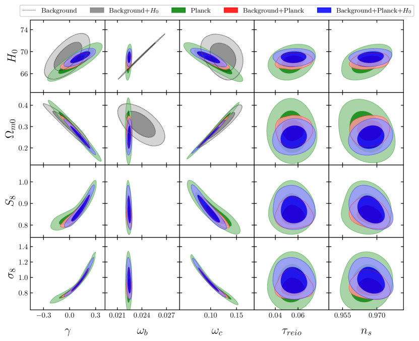
Figure 7: Rectangular plot with the free cosmological parameters, considering the analyses with WEC prior, using the datasets: Background, Background+$H_{0}$, Planck, Background+Planck and Background+Planck+$H_{0}$.

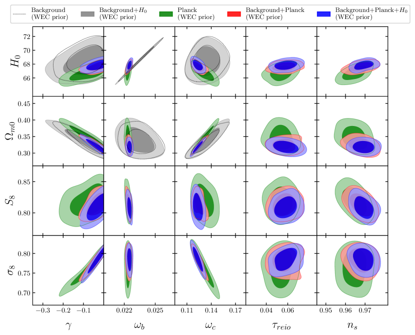
Figure 8: Rectangular plot with the free cosmological parameters, considering the analyses with WEC prior, using the datasets: Background, Background+$H_{0}$, Planck, Background+Planck and Background+Planck+$H_{0}$.

Figure 9 shows posteriors for several parameters without the use of a WEC prior. Figure 10 shows posteriors for several parameters with the use of a WEC prior.

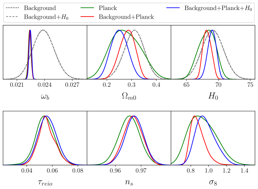
Figure 9: Posteriors for the free cosmological parameters, considering the analyses without WEC prior, using the datasets: Background, Background+$H_{0}$, Planck, Background+Planck and Background+Planck+$H_{0}$.

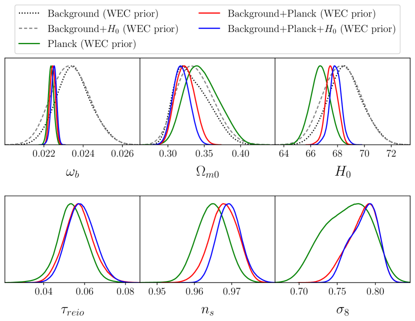
Figure 10: Posteriors for the free cosmological parameters, considering the analyses with WEC prior, using the datasets: Background, Background+$H_{0}$, Planck, Background+Planck and Background+Planck+$H_{0}$.

The confidence regions for $H_{0}$, $\Omega_{m0}$ and $\sigma_{8}$ are less restrictive without the WEC prior and more restrictive with it, being consistent with the Planck results [30] at 2$\sigma$ C.L.. Figures 7 and 8 show an anticorrelation between the interaction parameter $\gamma$ and the parameter $\Omega_{m0}$, and exhibits a correlation between the interaction parameter $\gamma$ and the parameters $\sigma_{8}$, $S_{8}$ and $H_{0}$. To interpret these correlations, it is useful to observe how the observables change as the involved parameters vary.

In Figure 11 are shown the expansion rate $H(z)$ (top panel) and the luminosity distance $D_{L}(z)$ (bottom panel) as a function of redshift for different values of $\gamma$. Even if we only consider the background, we can appreciate a compensatory effect between $\gamma$ and $\Omega_{m0}$. As $\Omega_{m0}$ increases, the growth of the Hubble parameter, which is related to the data of cosmic chronometers, decreases, since, in the absence of curvature, the contribution of dark energy increases. Since the smaller the $\gamma$ parameter, the greater the suppression of the dark matter energy density contribution (see Fig. 2), we find an anticorrelation between $\Omega_{m}$ and the interaction parameter. Consequently, the correlation between $\gamma$ and the Hubble constant is straightforward, as $H(z)$ increases with $H_{0}$. Similarly, the luminosity distance related to type Ia supernova data, since it incorporates the integral of $H(z)^{-1}$, increases with increasing $\Omega_{m0}$ parameter (or decreases with increasing $H_{0}$), just as it decreases with increasing the $\gamma$ parameter. It is possible to repeat the same evaluation for the angular distance $D_{A}$, related to the BAO data, since $D_{L}=(1+z)^{2}D_{A}$.

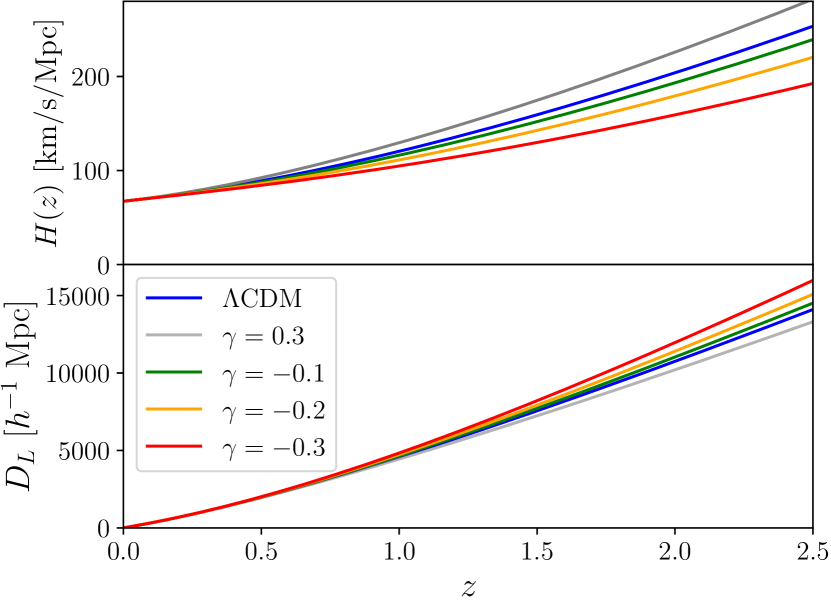
Figure 11: The top panel shows the expansion rate $H(z)$ as a function of redshift $z$ for different values of $\gamma$, while the bottom panel displays the luminosity distance $D_{L}$ for the same $\gamma$ values.

Figure 12 shows the temperature power spectrum as the parameter $\gamma$ varies, where it is possible to compare this behavior with that observed with changes in the parameter $\Omega_{m0}$ e $\sigma_{8}$. An increase in the value of $\Omega_{m0}$ brings forward the radiation epoch (see Figure 2), and through radiation driving, suppresses the power spectrum [57, 58]. Similarly, an increase in the parameter $\gamma$ also brings forward the radiation epoch, producing the same effect. Conversely, an increase in the $\sigma_{8}$ parameter corresponds to an increase in the amplitude of the scalar perturbations, or to an increase in the temperature anisotropies. This implies that in order to fit the data relating to the temperature fluctuations of the cosmic microwave background, we find an anticorrelation between the parameter $\gamma$ and the parameter $\Omega_{m0}$ and a correlation with the parameter $\sigma_{8}$ and therefore with the parameter $S_{8}$.

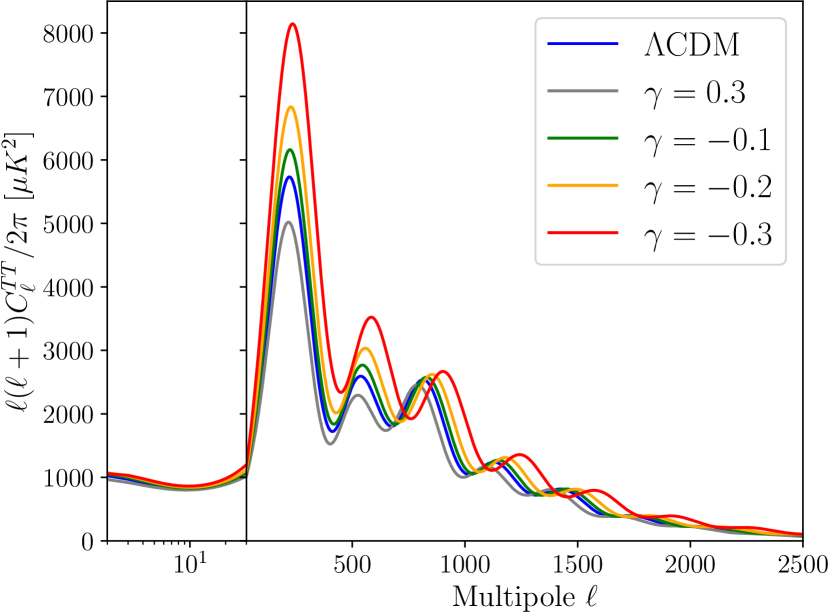
Figure 12: CMB temperature power spectra for different values of $\gamma$. We used the CLASS code, and for the $\Lambda$CDM model, we fixed the parameters $\gamma=0$, $\omega_{x}=-1$, $\omega_{c}=0.1200$, $\omega_{b}=0.02237$, and $h=0.6736$ [30], respectively.

Note that the same trends accompany other models that exhibit similar coupling physics [59, 10].

In Figure 13, the posterior results for the interaction parameter $\gamma$ are presented in two scenarios: without the use of a prior (left panel) and with the application of the WEC prior (right panel). For the case without prior, only when Planck data is not used, the mean value of $\gamma$ is negative, which prevents the violation of the WEC. On the other hand, when Planck data is used in the analysis, the mean value of $\gamma$ is slightly greater than zero, which means that the WEC will inevitably be violated in the future. In contrast, when the WEC prior is taken into account, the mean value of $\gamma$ is always negative, satisfying the WEC.

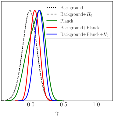
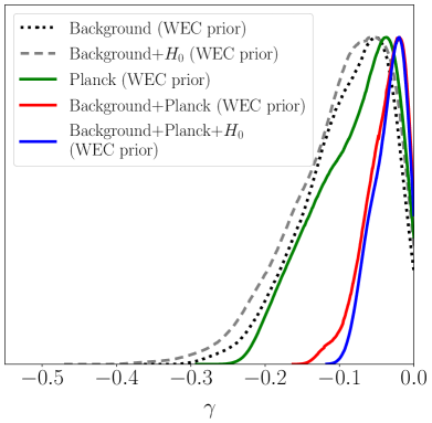
Figure 13: Posteriors for the interaction parameter $\gamma$: without the use of a WEC prior (left panel) and with the application of the WEC prior (right panel).

The results with WEC prior at $1\sigma$ C.L. for $\gamma$ do not satisfy the standard $\Lambda$CDM model. In all cases, the $\Lambda$CDM limit ($\gamma=0$) is satisfied within the $2\sigma$ C.L..

The right top panels of Figures 9 and 10 show the posteriors for $H_{0}$. Both for the case with the WEC prior and for the one without it, when the datasets Background, Background+$H_{0}$, and Planck are used there are weaker constraints on the Hubble constant, with a best-fit mean around $H_{0}\approx 68.5-68.8$ km s^-1 Mpc^-1, highlighting the need to add more data to these analyses. By combining Background data with Planck data, the constraints are improved. In Appendix A, we reproduced the $H_{0}$ tension between the analysis that includes the Planck data and the analysis that includes the background data only in the case of $\Lambda$CDM model ($\gamma=0$) (see Fig. 18). We noted that the tension is attenuated, especially in the case when the WEC prior is ignored.

In Figure 14, the plot for the plane $\sigma_{8}$ - $H_{0}$ is shown. In the case where the WEC prior was not used the constraints are weaker, while in the case the prior was adopted, the constraints are more stringent, and the estimates tend toward to lower value of $\sigma_{8}$.

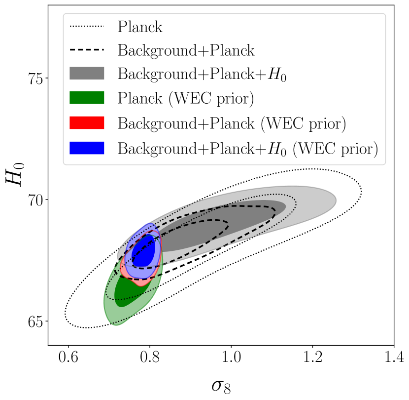
Figure 14: Plot of the parameter $\sigma_{8}$ versus the Hubble parameter $H_{0}$ without the WEC prior and with the WEC prior.

The results of the analyses with the WEC prior yield average values of approximately 67.4 and 0.78 for $H_{0}$ and $\sigma_{8}$, respectively. The preference for lower values of $\sigma_{8}$ alleviates the $\sigma_{8}$ tension between the primary CMB results from Planck 2018 [30] and the weak gravitational lensing observations from the KiDS-1000 cosmic shear survey [60].

Figure 15 shows the plot of the interaction parameter $\gamma$ versus the matter density parameter $\Omega_{m0}$ with and without the WEC prior. In the case without the WEC prior, all datasets have weak constraints on the parameters $\gamma$ and $\Omega_{m0}$, which appear to improve when the Background and $H_{0}$ data are combined with the Planck data. The inclusion of the WEC prior significantly improves the constraints of the parameters, resulting in higher values of $\Omega_{m0}$, which helps to alleviate the $S_{8}$ tension between the Planck CMB results and the estimates from the KiDS cosmic shear survey, as discussed in Refs. [30, 60, 61, 62].

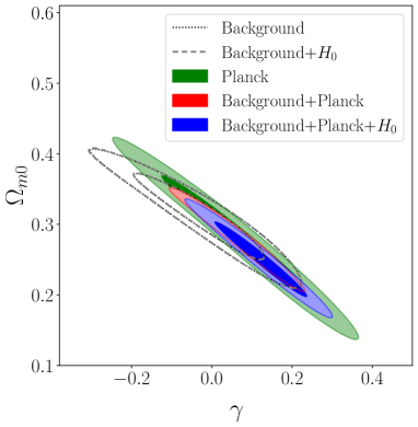
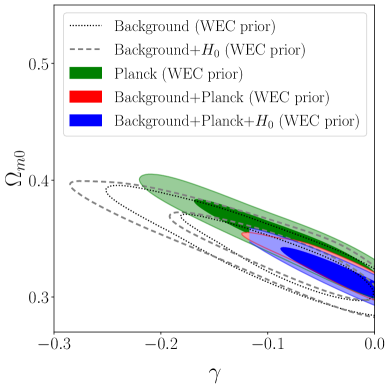
Figure 15: Plot of the interaction parameter $\gamma$ versus the matter density parameter $\Omega_{m0}$ without the WEC prior (left panel) and with the WEC prior (right panel).

Finally, in Figure 16, we present estimates of the quantity $S_{8}=\sigma_{8}\left({\Omega_{m0}}/{0.3}\right)^{1/2}$, with and without the WEC prior, using the datasets that include Planck. The results of the analyses without the WEC prior have weak constraints for $S_{8}$ and $\Omega_{m0}$. In contrast, the analyses with the WEC prior present good constraints, with mean values around 0.814 and 0.329 for $S_{8}$ and $\Omega_{m0}$, respectively. These results are in agreement at $2\sigma$ with the Planck 2018 results [30] for the $\Lambda$CDM model, and are also consistent with the results of weak gravitational lensing data from KiDS-1000 [60], as well as clustering and lensing data from the Dark Energy Survey [63, 64] at $\sim 3.5\sigma$ C.L.. The analyses with the WEC prior are also compatible with the results of the analyses for the $\Lambda$CDM model (see Appendix A, Tab. 5) at $1.2\sigma$ C.L.

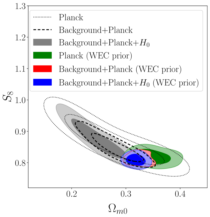
Figure 16: Plot of the matter density parameter $\Omega_{m0}$ versus the parameter $S_{8}$ without the WEC prior and with the WEC prior.

6 Conclusions

The standard model $\Lambda$CDM presents different problems, such as the cosmological constant problem, the cosmic coincidence, and the Hubble constant tension [5, 6, 7, 8, 9, 10, 11, 13], in this sense, several models and approaches have been proposed to better describe the nature of dark energy. Consequently, several interacting models have been suggested to capture possible interactions between the components of the dark sector of the universe. In this article, we explored an interacting model described by an interacting term proportional to $\rho_{x}^{2}/\left(\rho_{c}+\rho_{x}\right)$. The direction of the energy transfer depends on the sign of $Q$: when $Q<0$, the process of dark matter creation is enhanced and dark energy decays, whereas when $Q>0$, the opposite occurs. Here, we investigate the theoretical consistency of this class of cosmologies and show that for positive values of $\gamma$ ($\gamma>0$), which physically corresponds to an energy transfer from dark matter to dark energy, this particular model predicts a violation of the WEC, specifically a violation of $\rho_{c}\geq 0$, which will inevitably occur in the future evolution.

The analysis of the results was executed using the CLASS, MontePython, and GetDist codes, employing five different datasets, as described in Section 4. For all datasets, the results with the WEC prior showed negative values of $\gamma$ at 1$\sigma$ C.L, so excluding the standard $\Lambda$CDM model, which is reproduced by $\gamma=0$. However, for the 2$\sigma$ C.L. regions, the interaction parameter $\gamma=0$, hence the $\Lambda$CDM model is preferred.

Our results showed a notable anticorrelation between the interaction parameter $\gamma$ and $\Omega_{m0}$, as well as a correlation between $\gamma$ and the parameters $\sigma_{8}$, $S_{8}$, and $H_{0}$.

In the case without the WEC prior, adding the Background and $H_{0}$ data to the Planck data seems to alleviate the tension in $H_{0}$, which is related to the positive value of the interaction parameter $\gamma$. However, considering the WEC prior shifts the constraints to lower values of $H_{0}$, increasing the tension of the Hubble parameter. On the other hand, when the Background and $H_{0}$ data are combined with the Planck data, the constraints on $H_{0}$ and $\sigma_{8}$ are reasonably improved. The inclusion of the WEC prior significantly improves the parameter constraints, showing a preference for drastically lower values of $\sigma_{8}$, which alleviates the $\sigma_{8}$ tension between the results from the CMB data (Planck 2018) [30] and the weak gravitational lensing data (KiDS-1000) [60].

In the case without the WEC prior, all datasets show weak constraints on the parameters $\gamma$ and $\Omega_{m0}$, which improve when the Background and $H_{0}$ data are combined with the Planck data.

Our results show an anticorrelation between $\gamma$ and $\Omega_{m0}$. The inclusion of the WEC prior significantly improves the parameter constraints, resulting in higher values of $\Omega_{m0}$ and lower values of $\sigma_{8}$, which combined lead to a lower value of $S_{8}$, that is included between the values predicted by Planck 2018 [30], and the values predicted by the cosmic shear surveys [60, 61, 62]. In any case, our analysis exhibits that the model’s predictions are consistent with the current estimates of $\sigma_{8}$ and $S_{8}$ within $2\sigma$ C.L. regions with the Planck 2018 results.

Data availability

All data used are already publicly available and properly cited in this paper.

Appendix A Observational Results of the $\Lambda$CDM Model

Additionally, we will present a rectangular plot with the results for the $\Lambda$CDM model, as shown in Fig. 17 and the plot of posteriors in Fig. 18, along with Tables 4 and 5 displaying the main cosmological parameters within a $1\sigma$ C.L. for this model.

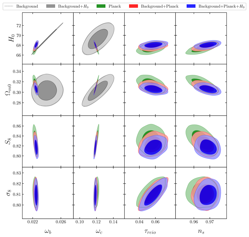
Figure 17: Rectangular plot with the free cosmological parameters in the $\Lambda$CDM model, using the datasets: Background, Background+$H_{0}$, Planck, Background+Planck and Background+Planck+$H_{0}$.

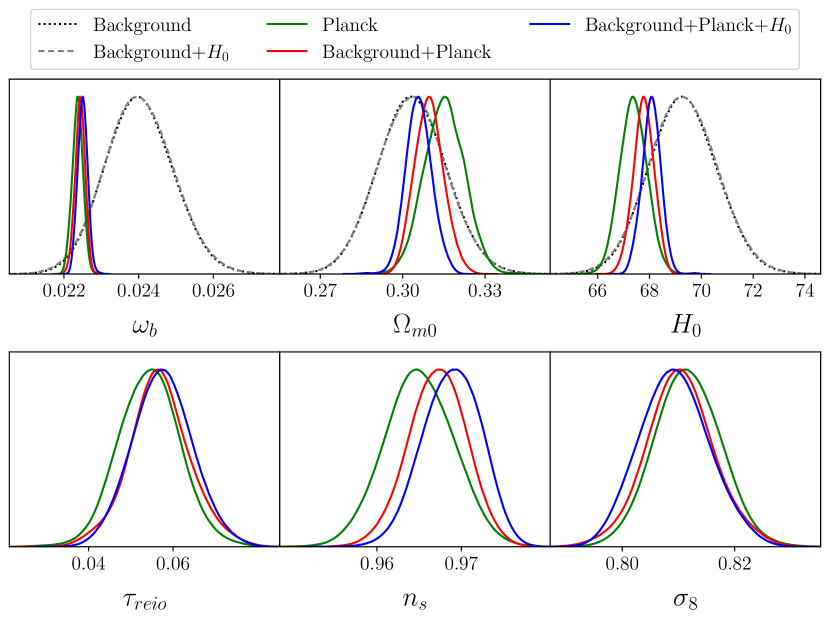
Figure 18: Posteriors for the free cosmological parameters in the $\Lambda$CDM model, using the datasets: Background, Background+$H_{0}$, Planck, Background+Planck and Background+Planck+$H_{0}$.

Table 4: Results of the statistical analysis of the $\Lambda$CDM model at $1\sigma$ C.L., using the datasets: Background, and Background+$H_{0}$.

Parameter	Background	Background+$H_{0}$
$\omega_{c}$	$0.1218^{+0.0078}_{-0.0078}$	$0.1217^{+0.0077}_{-0.0077}$
$H_{0}$	$69.3^{+1.3}_{-1.3}$	$69.3^{+1.3}_{-1.3}$
$\omega_{b}$	$0.02402^{+0.00091}_{-0.00091}$	$0.02402^{+0.00092}_{-0.00092}$
$\Omega_{m0}$	$0.304^{+0.012}_{-0.012}$	$0.303^{+0.013}_{-0.013}$

Table 5: Results of the statistical analysis of the $\Lambda$CDM model at $1\sigma$ C.L., using the datasets: Planck, Planck+Background, and Planck+Background+$H_{0}$.

Parameter	Planck	Background+Planck	Background+Planck+$H_{0}$
$100\theta{}_{s}$	$1.04189^{+0.00029}_{-0.00029}$	$1.04195^{+0.00029}_{-0.00029}$	$1.04207^{+0.00026}_{-0.00026}$
$\ln 10^{10}A_{s}$	$3.045^{+0.014}_{-0.014}$	$3.048^{+0.014}_{-0.014}$	$3.049^{+0.013}_{-0.016}$
$n_{s}$	$0.9650^{+0.0041}_{-0.0041}$	$0.9672^{+0.0035}_{-0.0035}$	$0.96889^{+0.0037}_{-0.0033}$
$\omega_{b}$	$0.02237^{+0.00014}_{-0.00014}$	$0.02243^{+0.00014}_{-0.00013}$	$0.02250^{+0.00013}_{-0.00013}$
$\omega_{c}$	$0.1200^{+0.0012}_{-0.0012}$	$0.11913^{+0.00088}_{-0.00088}$	$0.11858^{+0.00079}_{-0.00079}$
$\tau_{reio}$	$0.0544^{+0.0074}_{-0.0074}$	$0.0568^{+0.0073}_{-0.0073}$	$0.0575^{+0.0071}_{-0.0071}$
$H_{0}$	$67.38^{+0.53}_{-0.53}$	$67.78^{+0.40}_{-0.40}$	$68.08^{+0.37}_{-0.37}$
$\Omega_{m0}$	$0.3152^{+0.0073}_{-0.0073}$	$0.3096^{+0.0053}_{-0.0053}$	$0.3059^{+0.0048}_{-0.0048}$
$\sigma_{8}$	$0.8116^{+0.0059}_{-0.0059}$	$0.8103^{+0.0061}_{-0.0061}$	$0.8093^{+0.0061}_{-0.0061}$
$S_{8}$	$0.832^{+0.013}_{-0.013}$	$0.823^{+0.010}_{-0.010}$	$0.8171^{+0.0093}_{-0.0100}$

References

- Riess et al. [1998] A. G. Riess, A. V. Filippenko, P. Challis, et al., Observational evidence from supernovae for an accelerating universe and a cosmological constant, The Astronomical Journal 116 (1998) 1009–1038.
- Perlmutter et al. [1998] S. Perlmutter, G. Aldering, M. D. Valle, et al., Discovery of a supernova explosion at half the age of the universe, Nature 391 (1998) 51–54.
- Perlmutter et al. [1999] S. Perlmutter, G. Aldering, G. Goldhaber, et al., Measurements of and from 42 high-redshift supernovae, The Astrophysical Journal 517 (1999) 565–586.
- Lima [2004] J. A. S. Lima, Alternative dark energy models: an overview, Brazilian Journal of Physics 34 (2004) 194 – 200.
- Ellis et al. [2011] G. F. R. Ellis, H. van Elst, J. Murugan, J.-P. Uzan, On the trace-free einstein equations as a viable alternative to general relativity, Classical and Quantum Gravity 28 (2011) 225007.
- Sami [2009] M. Sami, A primer on problems and prospects of dark energy, arXiv e-prints (2009) arXiv:0904.3445.
- Velten et al. [2014] H. E. S. Velten, R. F. vom Marttens, W. Zimdahl, Aspects of the cosmological “coincidence problem”, The European Physical Journal C 74 (2014) 3160.
- Weinberg [1989] S. Weinberg, The cosmological constant problem, Rev. Mod. Phys. 61 (1989) 1–23.
- Zlatev et al. [1999] I. Zlatev, L. Wang, P. J. Steinhardt, Quintessence, cosmic coincidence, and the cosmological constant, Phys. Rev. Lett. 82 (1999) 896–899.
- von Marttens et al. [2019] R. von Marttens, L. Casarini, D. Mota, W. Zimdahl, Cosmological constraints on parametrized interacting dark energy, Physics of the Dark Universe 23 (2019) 100248. arXiv:1807.11380 [astro-ph.CO].
- Peebles and Ratra [2003] P. J. E. Peebles, B. Ratra, The cosmological constant and dark energy, Rev. Mod. Phys. 75 (2003) 559–606.
- Hou et al. [2017] S. Q. Hou, J. J. He, A. Parikh, et al., Non-extensive statistics to the cosmological lithium problem, The Astrophysical Journal 834 (2017) 165.
- Capozziello et al. [2024] S. Capozziello, G. Sarracino, G. De Somma, A critical discussion on the h0 tension, Universe 10 (2024).
- von Marttens et al. [2020] R. von Marttens, H. A. Borges, S. Carneiro, J. S. Alcaniz, W. Zimdahl, Unphysical properties in a class of interacting dark energy models, The European Physical Journal C 80 (2020) 1110.
- von Marttens et al. [2023] R. von Marttens, D. Barbosa, J. Alcaniz, One-parameter dynamical dark-energy from the generalized chaplygin gas, Journal of Cosmology and Astroparticle Physics 2023 (2023) 052.
- Di Valentino et al. [2020] E. Di Valentino, A. Melchiorri, O. Mena, S. Vagnozzi, Interacting dark energy in the early 2020s: A promising solution to the and cosmic shear tensions, Phys. Dark Univ. 30 (2020) 100666.
- Nunes et al. [2022] R. C. Nunes, S. Vagnozzi, S. Kumar, E. Di Valentino, O. Mena, New tests of dark sector interactions from the full-shape galaxy power spectrum, Phys. Rev. D 105 (2022) 123506.
- Kumar [2021] S. Kumar, Remedy of some cosmological tensions via effective phantom-like behavior of interacting vacuum energy, Physics of the Dark Universe 33 (2021) 100862.
- Di Valentino et al. [2020] E. Di Valentino, A. Melchiorri, O. Mena, S. Vagnozzi, Nonminimal dark sector physics and cosmological tensions, Phys. Rev. D 101 (2020) 063502.
- Rowland and Whittingham [2008] D. Rowland, I. B. Whittingham, Models of interacting dark energy, Monthly Notices of the Royal Astronomical Society 390 (2008) 1719–1726.
- Mishra et al. [2023] K. R. Mishra, S. K. J. Pacif, R. Kumar, K. Bamba, Cosmological implications of an interacting model of dark matter & dark energy, Physics of the Dark Universe 40 (2023) 101211.
- Riess et al. [2016] A. G. Riess, et al., A 2.4% Determination of the Local Value of the Hubble Constant, Astrophys. J. 826 (2016) 56.
- von Marttens et al. [2020] R. von Marttens, L. Lombriser, M. Kunz, V. Marra, L. Casarini, J. Alcaniz, Dark degeneracy i: Dynamical or interacting dark energy?, Physics of the Dark Universe 28 (2020) 100490.
- von Marttens et al. [2021] R. von Marttens, J. E. Gonzalez, J. Alcaniz, V. Marra, L. Casarini, Model-independent reconstruction of dark sector interactions, Phys. Rev. D 104 (2021) 043515.
- Ma and Bertschinger [1995] C.-P. Ma, E. Bertschinger, Cosmological perturbation theory in the synchronous and conformal Newtonian gauges, Astrophys. J. 455 (1995) 7–25.
- Majerotto et al. [2010] E. Majerotto, J. Väliviita, R. Maartens, Adiabatic initial conditions for perturbations in interacting dark energy models, Monthly Notices of the Royal Astronomical Society 402 (2010) 2344–2354.
- Yang et al. [2017] W. Yang, S. Pan, D. F. Mota, Novel approach toward the large-scale stable interacting dark-energy models and their astronomical bounds, Phys. Rev. D96 (2017) 123508.
- Caldera-Cabral et al. [2009] G. Caldera-Cabral, R. Maartens, B. M. Schaefer, The Growth of Structure in Interacting Dark Energy Models, JCAP 0907 (2009) 027.
- Kolb et al. [2006] E. W. Kolb, S. Matarrese, A. Riotto, On cosmic acceleration without dark energy, New Journal of Physics 8 (2006) 322.
- Planck Collaboration et al. [2020] Planck Collaboration, N. Aghanim, Y. Akrami, M. Ashdown, et al., Planck 2018 results - vi. cosmological parameters, A&A 641 (2020) A6.
- Scolnic et al. [2018] D. M. Scolnic, D. O. Jones, A. Rest, et al., The complete light-curve sample of spectroscopically confirmed SNe ia from pan-STARRS1 and cosmological constraints from the combined pantheon sample, The Astrophysical Journal 859 (2018) 101.
- Betoule et al. [2014] M. Betoule, R. Kessler, J. Guy, et al., Improved cosmological constraints from a joint analysis of the sdss-ii and snls supernova samples, Astronomy and Astrophysics 568 (2014) A22.
- Moresco et al. [2016] M. Moresco, L. Pozzetti, A. Cimatti, R. Jimenez, C. Maraston, L. Verde, D. Thomas, A. Citro, R. Tojeiro, D. Wilkinson, A 6% measurement of the hubble parameter atz0.45: direct evidence of the epoch of cosmic re-acceleration, Journal of Cosmology and Astroparticle Physics 2016 (2016) 014–014.
- Zhang et al. [2014] C. Zhang, H. Zhang, S. Yuan, S. Liu, T.-J. Zhang, Y.-C. Sun, Four new observational H(z) data from luminous red galaxies in the sloan digital sky survey data release seven, Research in Astronomy and Astrophysics 14 (2014) 1221–1233.
- Simon et al. [2005] J. Simon, L. Verde, R. Jimenez, Constraints on the redshift dependence of the dark energy potential, Phys. Rev. D71 (2005) 123001.
- Moresco et al. [2012] M. Moresco, et al., Improved constraints on the expansion rate of the Universe up to z 1.1 from the spectroscopic evolution of cosmic chronometers, JCAP 1208 (2012) 006.
- Stern et al. [2010] D. Stern, R. Jimenez, L. Verde, M. Kamionkowski, S. A. Stanford, Cosmic Chronometers: Constraining the Equation of State of Dark Energy. I: H(z) Measurements, JCAP 1002 (2010) 008.
- Moresco [2015] M. Moresco, Raising the bar: new constraints on the Hubble parameter with cosmic chronometers at , Monthly Notices of the Royal Astronomical Society, Letters 450 (2015) L16–L20.
- Bassett and Hlozek [2009] B. A. Bassett, R. Hlozek, Baryon acoustic oscillations, 2009. arXiv:0910.5224.
- Eisenstein et al. [2007] D. J. Eisenstein, H.-J. Seo, M. White, On the Robustness of the Acoustic Scale in the Low-Redshift Clustering of Matter, APJ 664 (2007) 660--674.
- Aizpuru et al. [2021] A. Aizpuru, R. Arjona, S. Nesseris, Machine learning improved fits of the sound horizon at the baryon drag epoch, Phys. Rev. D 104 (2021) 043521.
- Eisenstein et al. [2005] D. J. Eisenstein, I. Zehavi, D. W. Hogg, et al., Detection of the baryon acoustic peak in the large-scale correlation function of SDSS luminous red galaxies, The Astrophysical Journal 633 (2005) 560--574.
- Haridasu et al. [2018] B. S. Haridasu, V. V. Luković, N. Vittorio, Isotropic vs. anisotropic components of bao data: a tool for model selection, Journal of Cosmology and Astroparticle Physics 2018 (2018) 033.
- Anderson et al. [2014] L. Anderson, et al. (BOSS), The clustering of galaxies in the SDSS-III Baryon Oscillation Spectroscopic Survey: baryon acoustic oscillations in the Data Releases 10 and 11 Galaxy samples, Mon. Not. Roy. Astron. Soc. 441 (2014) 24--62.
- Ross et al. [2015] A. J. Ross, L. Samushia, C. Howlett, W. J. Percival, A. Burden, M. Manera, The clustering of the SDSS DR7 main Galaxy sample – I. A 4 per cent distance measure at , Mon. Not. Roy. Astron. Soc. 449 (2015) 835--847.
- Font-Ribera et al. [2014] A. Font-Ribera, D. Kirkby, N. Busca, et al., Quasar-lyman forest cross-correlation from boss: Baryon acoustic oscillations, Journal of Cosmology and Astroparticle Physics 2014 (2014) 027.
- Planck Collaboration et al. [2020] Planck Collaboration, Aghanim, N., Akrami, Y., Ashdown, M., et al., Planck 2018 results - v. cmb power spectra and likelihoods, A&A 641 (2020) A5.
- Brinckmann and Lesgourgues [2019] T. Brinckmann, J. Lesgourgues, Montepython 3: Boosted mcmc sampler and other features, Physics of the Dark Universe 24 (2019) 100260.
- Audren et al. [2013] B. Audren, J. Lesgourgues, K. Benabed, S. Prunet, Conservative constraints on early cosmology with monte python, Journal of Cosmology and Astroparticle Physics 2013 (2013) 001.
- Blas et al. [2011] D. Blas, J. Lesgourgues, T. Tram, The cosmic linear anisotropy solving system (CLASS). part II: Approximation schemes, Journal of Cosmology and Astroparticle Physics 2011 (2011) 034--034.
- Metropolis et al. [1953] N. Metropolis, A. W. Rosenbluth, M. N. Rosenbluth, A. H. Teller, E. Teller, Equation of state calculations by fast computing machines, The Journal of Chemical Physics 21 (1953) 1087--1092.
- Hastings [1970] W. K. Hastings, Monte Carlo sampling methods using Markov chains and their applications, Biometrika 57 (1970) 97--109.
- Vats and Knudson [2018] D. Vats, C. Knudson, Revisiting the Gelman-Rubin Diagnostic, arXiv e-prints (2018) arXiv:1812.09384.
- Gelman and Rubin [1992] A. Gelman, D. B. Rubin, Inference from iterative simulation using multiple sequences, Statist. Sci. 7 (1992) 457--472.
- Lewis [2019] A. Lewis, Getdist: a python package for analysing monte carlo samples, 2019. arXiv:1910.13970.
- Lewis [2019] A. Lewis, GetDist: Monte Carlo sample analyzer, Astrophysics Source Code Library, record ascl:1910.018, 2019.
- Hu and Dodelson [2002] W. Hu, S. Dodelson, Cosmic microwave background anisotropies, Annual Review of Astronomy and Astrophysics 40 (2002) 171--216.
- Wands et al. [2016] D. Wands, O. F. Piattella, L. Casarini, Physics of the cosmic microwave background radiation, in: J. C. Fabris, O. F. Piattella, D. C. Rodrigues, H. E. Velten, W. Zimdahl (Eds.), The Cosmic Microwave Background, Springer International Publishing, Cham, 2016, pp. 3--39.
- vom Marttens et al. [2017] R. vom Marttens, L. Casarini, W. Zimdahl, W. Hipólito-Ricaldi, D. Mota, Does a generalized chaplygin gas correctly describe the cosmological dark sector?, Physics of the Dark Universe 15 (2017) 114--124.
- Heymans, Catherine et al. [2021] Heymans, Catherine, Tröster, Tilman, Asgari, Marika, et al., Kids-1000 cosmology: Multi-probe weak gravitational lensing and spectroscopic galaxy clustering constraints, A&A 646 (2021) A140.
- Joudaki et al. [2017a] S. Joudaki, A. Mead, C. Blake, et al., KiDS-450: testing extensions to the standard cosmological model, Monthly Notices of the Royal Astronomical Society 471 (2017a) 1259--1279.
- Joudaki et al. [2017b] S. Joudaki, C. Blake, A. Johnson, A. Amon, et al., KiDS-450 + 2dFLenS: Cosmological parameter constraints from weak gravitational lensing tomography and overlapping redshift-space galaxy clustering, Monthly Notices of the Royal Astronomical Society 474 (2017b) 4894--4924.
- Troxel et al. [2018] M. A. Troxel, N. MacCrann, J. Zuntz, et al. (Dark Energy Survey Collaboration), Dark energy survey year 1 results: Cosmological constraints from cosmic shear, Phys. Rev. D 98 (2018) 043528.
- Amon et al. [2022] A. Amon, D. Gruen, M. A. Troxel, N. MacCrann, et al. (DES Collaboration), Dark energy survey year 3 results: Cosmology from cosmic shear and robustness to data calibration, Phys. Rev. D 105 (2022) 023514.