Easy better quantum process tomography

Abstract

Quantum process tomography (QPT), used to estimate the linear map that best describes a quantum operation, is usually performed using a priori assumptions about state preparation and measurement (SPAM), which yield a biased and inconsistent estimator. This estimate can be made more accurate and less biased by incorporating SPAM-calibration data. Unobservable properties of the SPAM operations introduce a small gauge freedom that can be regularized using the a priori SPAM. We give an explicit correction procedure for standard linear-inversion QPT and overcomplete linear-inversion QPT, and describe how to extend it to statistically principled estimators like maximum likelihood estimation.

Quantum process tomography (QPT) Chuang and Nielsen (1997); O’Brien et al. (2004); Hashim et al. (2024) is used to estimate the linear map that best describes a quantum operation. Standard QPT is vulnerable to state preparation and measurement or “SPAM” Magesan et al. (2012) error Quesada et al. (2013); Merkel et al. (2013); Stark (2014); Blume-Kohout et al. (2013); Greenbaum (2015). Unless the tomographer knows and uses exactly correct models for the initial states and final measurements used to probe the unknown operation, QPT will yield biased, inaccurate estimates. Gate set tomography (GST) Merkel et al. (2013); Greenbaum (2015); Blume-Kohout et al. (2017); Nielsen et al. (2021) was developed to eliminate this problem, but because GST requires more experimental effort and more complicated analysis than QPT, it is sometimes viewed as “too much work”. QPT is still commonly used despite its known flaws.

This paper shows how to eliminate QPT’s SPAM-induced inaccuracy with minimal extra effort. This “better QPT” algorithm requires only $2\times$ as much experimental data and is just as simple as standard QPT. It uses the essential idea behind GST but applies it to estimate a single operation. It acknowledges the gauge freedom Blume-Kohout et al. (2017); Proctor et al. (2017); Rudnicki et al. (2018); Lin et al. (2019); Chen et al. (2023); Nielsen et al. (2021) associated with GST (and ignored by QPT), but deals with it in the simplest possible way. If the a priori SPAM operations were rank-1 (perfect), then the corrected estimate will be not just more accurate, but less noisy.

I Standard QPT

QPT estimates an unknown operation $G$ on a quantum system with $d$-dimensional Hilbert space $\mathcal{H}$ by

1. choosing a set of known quantum states, described by $d\times d$ density matrices $\{\overline{\rho}_{j}\}$, to which the unknown operation will be applied,

2. choosing a set of known quantum measurements, described by positive operator-valued measures (POVMs) with outcomes described by $d\times d$ positive semi-definite “effects” $\{\overline{E}_{i}\}$, to perform on the transformed states,

3. repeatedly preparing each $\overline{\rho}_{j}$, applying $G$, and performing each of the various measurements, so that for every $(i,j)$, the probability $P_{i,j}$ of observing effect $\overline{E}_{i}$ given $G[\overline{\rho}_{j}]$ can be estimated to reasonable precision.

The resulting data can be analyzed by representing each density matrix $\overline{\rho}_{j}$ as a column vector $\left|\overline{\rho}_{j}\right\rrangle$ in the $d^{2}$-dimensional Hilbert-Schmidt space $\mathcal{B}(\mathcal{H})$ of operators and each effect $\overline{E}_{i}$ as a row vector $\left\llangle\overline{E}_{i}\right|$ in $\mathcal{B}(\mathcal{H})$, and then arranging the probabilities $P_{i,j}$ into a matrix that can be written using Born’s rule ($\mathrm{Pr}(E|\rho)=\mathrm{Tr}[E\rho]$) and the Hilbert-Schmidt inner product ($\left\llangle A|B\right\rrangle=\mathrm{Tr}[A^{\dagger}B]$) as

$$P_{i,j}\equiv\mathrm{Pr}\left(\overline{E}_{i}|G[\overline{\rho}_{j}]\right)=\left\llangle\overline{E}_{i}\right|G\left|\overline{\rho}_{j}\right\rrangle.$$

An easy and elegant way to write this is by constructing two matrices,

$$M_{0} = \left(\begin{array}[]{c}\left\llangle\overline{E}_{1}\right|\\ \left\llangle\overline{E}_{2}\right|\\ \vdots\end{array}\right),$$ (4)

$$S_{0} = \left(\left|\overline{\rho}_{1}\right\rrangle\left|\overline{\rho}_{2}\right\rrangle\ldots\right),$$

so that

$$P=M_{0}GS_{0}.$$ (5)

Now, if $\hat{P}$ contains the estimated probabilities, then the “linear inversion” estimate of the unknown process is simply

$$\hat{G}_{0}=M_{0}^{-1}\hat{P}S_{0}^{-1}.$$ (6)

More sophisticated estimators like maximum likelihood estimation Hradil (1997); Banaszek et al. (1999); James et al. (2001); Wasserman (2013) tweak this simple algorithm to mitigate the effects of significant finite-sample fluctuations in $\hat{P}$, which include violation of the complete positivity constraint $\left(\hat{G}\otimes 1\!\mathrm{l}\right)[\left|\mathrm{\textsc{bell}}\right\rangle\!\!\left\langle\mathrm{\textsc{bell}}\right|]\geq 0$ and inconsistency between probabilities associated with “overcomplete” sets of states and/or effects.

II The problem with QPT

QPT works fine if the $\overline{\rho}_{j}$ and $\overline{E}_{i}$ do, in fact, represent the true states and effects used in the QPT experiment. But most QPT experiments are analyzed under the implausible assumption that each state preparation and measurement (SPAM) operation – the true $\{\rho_{j}\}$ and $\{E_{i}\}$ – is exactly equal to the rank-1 state $\overline{\rho}_{j}$ or effect $\overline{E}_{i}$ describing the experimenter’s intent. This model is obviously wrong, because experiments are noisy. It yields incorrect $M_{0}$ and $S_{0}$ matrices that (in turn) yield incorrect and potentially misleading estimates $\hat{G}_{0}$.

Some QPT experiments do better by attempting to model the SPAM operations that make up $M_{0}$ and $S_{0}$ as realistically noisy operations, inferred from data. However, the canonical way to estimate a density matrix is quantum state tomography, which relies on known POVM effects…and the canonical way to estimate a POVM is quantum measurement tomography, which relies on known states. This creates an obvious circularity, to which no really satisfactory solution is known. It is now understood that states and measurements literally can’t be fully learned or estimated, because controllable quantum systems have a gauge symmetry Blume-Kohout et al. (2017); Proctor et al. (2017); Rudnicki et al. (2018); Lin et al. (2019); Chen et al. (2023); Nielsen et al. (2021).

In principle, this gauge symmetry creates existential problems for state, measurement, and process tomography. Yet all three of these protocols are still regularly performed and their results published, suggesting the gauge problem is not as unsolvable in practice as it is in principle.

III Better QPT

QPT can be improved by learning about the SPAM operations and adjusting the estimate $\hat{G}$ with that knowledge. This can be done by performing an additional “process tomography on nothing” experiment to estimate each of the probabilities

$$I_{i,j}\equiv\mathrm{Pr}(E_{i}|\rho_{j})=\left\llangle E_{i}|\rho_{j}\right\rrangle.$$

The unknown SPAM operations are now modeled by defining two unknown matrices

$$M = \left(\begin{array}[]{c}\left\llangle E_{1}\right|\\ \left\llangle E_{2}\right|\\ \vdots\end{array}\right),$$ (10)

$$S = \left(\left|\rho_{1}\right\rrangle\left|\rho_{2}\right\rrangle\ldots\right),$$

of which $M_{0}$ and $S_{0}$ are just a priori estimates. There are now two matrices of observable probabilities,

$$I = MS,$$

$$P = MGS.$$

If the a priori guesses about the $\{\rho_{j}\}$ and $\{E_{i}\}$ were correct – i.e., $M=M_{0}$ and $S=S_{0}$, then taking data and estimating the elements of $I$ will yield $\hat{I}=M_{0}S_{0}$ to within finite-sample fluctuations (error bars). If this is observed, the assumptions of standard QPT are validated and Eq. 6 can be used directly.

Otherwise, $\hat{I}$ can be used to construct a $\hat{G}$ that is more accurate than $\hat{G}_{0}$. Writing

$$I=M_{0}\mathcal{E}S_{0},$$

defines a SPAM error superoperator $\mathcal{E}$ that captures the SPAM operations’ deviation from expectations. It can be estimated as

$$\hat{\mathcal{E}}=M_{0}^{-1}\hat{I}S_{0}^{-1}.$$

Note that $\mathcal{E}$ is not required to be a physical process (i.e., a completely positive, trace-preserving map); it merely describes the errors in the SPAM operations.

If the states $\{\rho_{j}\}$ were known to be perfect ($S=S_{0}$), then the rows of $M=M_{0}\mathcal{E}$ would reveal the noisy measurement effects $\{E_{i}\}$. Similarly, if the effects $\{E_{i}\}$ were known to be perfect ($M=M_{0}$) then the columns of $S=\mathcal{E}S_{0}$ would reveal the noisy states $\{\rho_{j}\}$.

In practice, both are noisy. The data cannot tell us how to divide the SPAM error described by $\hat{\mathcal{E}}$ between $M$ (measurements) and $S$ (states). In principle, any factorization $\hat{\mathcal{E}}=\alpha\beta$ yields a valid theory about the SPAM operations:

$$\hat{S} = \beta S_{0},$$

$$\hat{M} = M_{0}\alpha=M_{0}\mathcal{E}\beta^{-1},$$

and in turn a valid theory about $G$:

$$\hat{G} = \hat{M}^{-1}\hat{P}\hat{S}^{-1}$$

$$= \alpha^{-1}M_{0}^{-1}\hat{P}S_{0}^{-1}\beta^{-1}$$

$$= \alpha^{-1}\hat{G}_{0}\beta^{-1}$$

$$= \beta\hat{\mathcal{E}}^{-1}\hat{G}_{0}\beta^{-1}.$$

But this constitutes excessive respect for gauge freedom. We should respect the a priori estimates $M\approx M_{0}$ and $S\approx S_{0}$, while adjusting them to respect the data. By choosing $\beta=\hat{\mathcal{E}}^{1/2}$, we can divide the SPAM error $\hat{\mathcal{E}}$ equally between states and effects:

$$\hat{S} = \hat{\mathcal{E}}^{1/2}S_{0}$$

$$\hat{M} = M_{0}\hat{\mathcal{E}}^{1/2}$$ (11)

$$\Rightarrow \hat{G}=\hat{\mathcal{E}}^{-1/2}\hat{G}_{0}\hat{\mathcal{E}}^{-1/2}.$$

If there is reason to believe that either state preparation or measurement is more error-prone, then it is equally valid to divide the SPAM error unequally by choosing $\beta=\hat{\mathcal{E}}^{p}$ for some $p\in[0,1]$ so that:

$$\hat{S} = \hat{\mathcal{E}}^{p}S_{0}$$

$$\hat{M} = M_{0}\hat{\mathcal{E}}^{1-p}$$

$$\Rightarrow \hat{G}(p)=\hat{\mathcal{E}}^{p-1}\hat{G}_{0}\hat{\mathcal{E}}^{-p}.$$

If the observed SPAM error $\hat{\mathcal{E}}$ commutes with $\hat{G}_{0}$ – e.g., if it is a depolarizing channel – then these options all coincide. Even when they do not, the spectrum of $\hat{G}$ is independent of $p$, indicating that unless $\hat{\mathcal{E}}$ is very far from the identity, the choice of gauge is relatively unimportant.

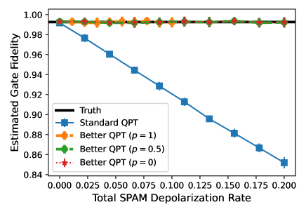
Figure 1: Comparative accuracy of standard and SPAM-corrected QPT: We compared the accuracy of standard QPT (blue) and SPAM-adjusted QPT (orange, green, red) by simulating both forms of QPT on an $X_{\pi/2}$ gate with $1\%$ depolarizing noise, with 5000 shots per circuit (see main text for details). To quantify accuracy, we used the process matrix estimated by each protocol to estimate the noisy gate’s fidelity with a noiseless $X_{\pi/2}$ unitary, and plotted the error in this estimated fidelity as a function of the strength of depolarizing SPAM noise (top panel) and coherent SPAM noise (bottom panel; see main text for details). When performing SPAM-corrected QPT, we assigned a fraction $p=0$, $p=0.5$, and $p=1$ (orange, green, and red, respectively) of the observed SPAM error to state preparation, and the remainder to measurement. This gauge choice had no effect for depolarizing SPAM error, but a weak effect for coherent SPAM errors.

IV Simulations

To demonstrate benefits of this protocol, we simulated standard and better QPT with SPAM errors on a single-qubit $X_{\pi/2}$ gate with $1\%$ uniform depolarizing noise (i.e., an ideal $X_{\pi/2}$ unitary followed by the error process $\mathcal{D}_{\gamma}[\rho]=\gamma\rho+(1-\gamma)\mathbb{I}/3$ with $\gamma=0.99$). We added two kinds of SPAM noise to an experiment in which, in the absence of noise, both the input states and the measured effects were given by Pauli eigenstates $\{\left|+_{x}\right\rangle\!\!\left\langle+_{x}\right|,\left|-_{x}\right\rangle\!\!\left\langle-_{x}\right|,\left|+_{y}\right\rangle\!\!\left\langle+_{y}\right|,\left|+_{z}\right\rangle\!\!\left\langle+_{z}\right|\}$.

The first “depolarizing” error model applied uniform depolarization ($\mathcal{D}_{\gamma}$) with varying strength $1-\gamma$ to both state preparation and measurement. The total SPAM depolarization rate is therefore $1-2\gamma$, since both states and measurements are depolarized. The second “coherent” error model left the measurement effects noise-free, but replaced each ideal input state with a positive real superposition of the intended state and the orthogonal state given by $\left|\psi_{\phi}\right\rangle=\cos\phi\left|\psi\right\rangle+\sin\phi\left|\psi_{\perp}\right\rangle$ where $\left|\psi\right\rangle$ is the intended state, $\left|\psi_{\perp}\right\rangle$ the unique orthogonal state, and $\phi$ was varied between $0$ and $0.1$ radians (producing a maximum infidelity of $\sin^{2}\phi\approx 1\%$).

We simulated 50 runs of QPT experiments with 5000 shots of each circuit (12 circuits for standard QPT, 24 for SPAM-corrected QPT). All error bars are $1\sigma$ and derived from the variance of the 50 repetitions. Because QPT is often used to estimate an as-implemented gate’s fidelity with its ideal target, we quantify the accuracy of each method by computing and reporting the difference between the true value of that fidelity and the value computed from the QPT estimate.

Figure 1 shows the accuracy of the process matrices estimated by standard and better process tomography, for both SPAM error models, as a function of SPAM error magnitude ($2\gamma$ or $\phi$). Because it depends on the tomographer’s a priori division of SPAM error between state preparation and measurement, we show the results of three different divisions, in which $p=0$, $p=0.5$, and $p=1$ of the SPAM error (respectively) is assigned to state preparation. In all cases, SPAM-corrected QPT yields better accuracy than standard QPT. For depolarizing SPAM error (top panel) it doesn’t matter how SPAM error is divided, but for the particular coherent errors considered here, guessing wrong about the division of error causes a small degradation in accuracy.

The division of SPAM error is a choice of gauge. Figure 1 shows that even when a gauge-variant quantity (fidelity) is computed, this gauge choice has a relatively minor impact when the SPAM error is small. But if we focus on gauge-invariant properties – e.g., the eigenvalues of the estimated process matrix – the impact of this gauge choice should vanish entirely. Figure 2 confirms that SPAM-corrected QPT estimates gate eigenvalues very accurately, and (unlike standard QPT) is completely immune to SPAM error. We quantified error in the estimated eigenvalues by $\delta=\frac{1}{4}\sum_{i}|\lambda_{i}-\tilde{\lambda}_{i}|$ where $\lambda_{i}$ are the true eigenvalues and $\tilde{\lambda}_{i}$ the estimates. We also found that the residual error in the eigenvalues declines to zero as the number of shots is increased (not shown).

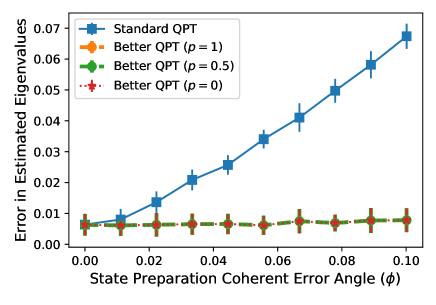
Figure 2: Error in estimated gate eigenvalues: Gauge-invariant quantities like the eigenvalues of the estimated superoperator (transfer matrix) should be independent of how SPAM error is divided. We analyzed the results of simulated standard and SPAM-corrected QPT to determine how inaccurately they estimated gate eigenvalues, using the figure of merit $\delta=\frac{1}{4}\sum_{i}|\lambda_{i}-\tilde{\lambda}_{i}|$, where $\lambda_{i}$ are the true eigenvalues and $\tilde{\lambda}_{i}$ the estimates. Standard QPT’s inaccuracy grows with SPAM error, while SPAM-corrected QPT’s accuracy is unaffected by SPAM error.

V Overcomplete data

The derivation above assumed the use of states and measurements that are informationally complete, not overcomplete. If $K>d^{2}$ states and/or effects are considered, then the matrices $M$ and/or $S$ become rectangular, and do not have inverses. In standard QPT, Eq. 5 ($P=M_{0}GS_{0}$) becomes overconstrained and has no solutions, because the rank of $M_{0}GS_{0}$ is at most $d^{2}$, while $P$ can have rank $K$.

The easiest way to deal with this is with ordinary least-squares fitting, finding the $\hat{G}$ that minimizes $\|M_{0}GS_{0}-P\|_{2}^{2}$. This admits a closed-form solution, given by replacing matrix inverses with Moore-Penrose pseudoinverses, e.g.

$$M_{0}^{+} \equiv (M_{0}^{\dagger}M_{0})^{-1}M_{0}^{\dagger}$$

$$S_{0}^{+} \equiv S_{0}^{\dagger}(S_{0}S_{0}^{\dagger})^{-1}.$$

The standard OLS QPT estimate of $G$ for overcomplete data is therefore

$$\hat{G}_{0}=M_{0}^{+}\hat{P}S_{0}^{+}.$$

This estimate can also be SPAM-corrected using the information obtained by measuring $I=MS$. However, the procedure (and its derivation) are slightly more complicated and illuminating.

Since $M$ and $S$ are (respectively) $K\times d^{2}$ and $d^{2}\times K$ matrices, the $K\times K$ matrix of empirical probabilities $I=MS$ has rank at most $d^{2}<K$. However, an experimentally estimated $\hat{I}$ will generally be full-rank because of (1) sampling error in the empirical probabilities, and/or (2) inadvertent manipulation of a larger state space than intended (a form of non-Markovian error). If $\mathrm{rank}(\hat{I})>d^{2}$, then the only way to find $M$ and $S$ satisfying $MS=\hat{I}$ is by “truncating” $\hat{I}$ to the closest rank-$d^{2}$ matrix. This can be done by performing a singular value decomposition and replacing $\hat{I}$’s smallest $K-d^{2}$ singular values with 0.

Truncation also improves accuracy, under the assumption that deviations from rank-$d^{2}$ are caused by finite-sample fluctuations. For this reason, it is advantageous (though not required) to truncate $\hat{P}$ as well.

Once truncated, $\hat{I}$ can be factored as $\hat{I}=MS$ for properly sized $M$ and $S$. But $M$ and $S$ are not unique in this factorization. If $MS=\hat{I}$ then $(MQ)(Q^{-1}S)=\hat{I}$ as well, for any invertible $d^{2}\times d^{2}$ matrix $Q$. We want one for which $M\approx M_{0}$ and $S\approx S_{0}$. We could minimize $\|M-M_{0}\|_{2}$ by choosing

$$S_{\mathrm{m-opt}} \equiv M_{0}^{+}\hat{I},$$ (12)

$$M_{\mathrm{m-opt}} \equiv \hat{I}S_{\mathrm{m-opt}}^{+}.$$ (13)

This is a valid factorization – i.e., $M_{\mathrm{m-opt}}S_{\mathrm{m-opt}}=\hat{I}S_{\mathrm{m-opt}}^{+}S_{\mathrm{m-opt}}=\hat{I}$ – because (1) $S_{\mathrm{m-opt}}^{+}S_{\mathrm{m-opt}}$ is the product of a rank-$d^{2}$ matrix and its pseudo-inverse and must therefore be a rank-$d^{2}$ projector, and (2) $S_{\mathrm{m-opt}}^{+}S_{\mathrm{m-opt}}=S_{\mathrm{m-opt}}^{+}M_{0}^{+}\hat{I}$ necessarily annihilates any vector in the orthogonal complement of $\hat{I}$’s ($d^{2}$-dimensional) row space. Therefore, $S_{\mathrm{m-opt}}^{+}S_{\mathrm{m-opt}}$ must be the projector onto the row space of $\hat{I}$.

Alternatively, we could minimize $\|S-S_{0}\|_{2}$ by choosing

$$M_{\mathrm{s-opt}} \equiv \hat{I}S_{0}^{+},$$ (14)

$$S_{\mathrm{s-opt}} \equiv M_{\mathrm{s-opt}}^{+}\hat{I}.$$ (15)

To split the difference as in the previous section, we can write

$$\hat{I}=M_{\mathrm{m-opt}}\hat{\mathcal{E}}S_{\mathrm{s-opt}},$$

where $\hat{\mathcal{E}}$ is once again a $d^{2}\times d^{2}$ matrix. We can then extract $\hat{\mathcal{E}}$ as

$$\hat{\mathcal{E}}=M_{\mathrm{m-opt}}^{+}\hat{I}S_{\mathrm{s-opt}}^{+},$$ (16)

and obtain good estimates of $M$ and $S$ as

$$\hat{M}=M_{\mathrm{m-opt}}\hat{\mathcal{E}}^{1/2},$$ (17)

$$\hat{S}=\hat{\mathcal{E}}^{1/2}S_{\mathrm{s-opt}}.$$ (18)

Finally, using these estimates of $M$ and $S$, we can analyze the process tomography data ($P$) as

$$\hat{G}=\hat{M}^{+}\hat{P}\hat{S}^{+}.$$ (19)

It is possible to expand Eq. 19 using the definition of the pseudoinverse and Eqs. 17-18 and their predecessors (Eqs. 12-16), but the nested pseudoinverses don’t simplify. However, applying the uncontrolled approximation $(AB)^{+}\approx B^{+}A^{+}$, yields the suggestive approximation

$$\hat{G}\approx\hat{\mathcal{E}}^{-1/2}M_{0}^{+}\Pi_{c}\hat{P}\Pi_{r}S_{0}\hat{\mathcal{E}}^{-1/2},$$

where $\Pi_{c}$ and $\Pi_{r}$ project (respectively) onto $\hat{I}$’s column and row spaces, respectively. This mirrors Eq. 11, but with the addition of projections onto the most active subspaces of $\hat{I}$ (and optionally also of $\hat{P}$).

VI Principled statistical estimation

The analysis above equates “estimation” with linear regression via ordinary least squares. This is an oversimplification, although a very useful one. The estimators in Eqs. 11 and 19 can absolutely be used in practice, but they will be suboptimal for at least three reasons.

1. In Eq. 19, the matrix of empirical probabilities for QPT ($\hat{P}$) is projected onto the support of $\hat{I}$ by $\hat{I}^{+}\hat{I}$, because in a previous step we used $\hat{I}$ to identify the active subspaces supporting $M$ and $S$. Since $K>d^{2}$ states or effects in a $d^{2}$-dimensional space cannot be linearly independent, some subspace restriction is necessary. But $\hat{P}$ also contains information about active subspaces, which is not used because $\hat{I}$ and $\hat{P}$ are analyzed separately.

2. The estimated probabilities in $\hat{I}$ and $\hat{P}$ have varying precisions, because the Fisher information of multinomial parameters varies with the parameter. Ordinary least squares ignores this.

3. The process estimate $\hat{G}$ and/or the SPAM estimates $\hat{M}$ and $\hat{S}$ may violate physical constraints (each $\rho_{i}$ and $E_{j}$ must be positive semidefinite, and $G$ must be completely positive and trace-preserving, or CPTP). These constraints are nontrivial, and cannot usually be enforced in closed form (except in the special case of Ref. Smolin et al. (2012)).

These deficiencies can all be addressed by replacing closed-form linear regression with numerical algorithms for statistical estimation that fit unknown parameters to data using statistical principles such as maximum likelihood estimation (MLE) Hradil (1997); Banaszek et al. (1999); James et al. (2001); Wasserman (2013). Principled statistical estimators typically yield more accurate results than least-squares regression.

There are at least three ways to integrate sophisticated statistical estimators with the “better QPT” workflow described above.

1. Independent estimation of $\mathcal{E}$ and $G_{0}$: Use a statistical principle (e.g. MLE) to estimate SPAM error $\hat{\mathcal{E}}$ from data in $\hat{I}$ and to estimate $\hat{G}_{0}$ from data in $\hat{P}$, and then compute $\hat{G}$ using Eq. 11 or 19. This is the easiest approach, but relative näive – e.g., $\hat{G}$ may not satisfy positivity.

2. Sequential estimation of SPAM and $G$: Use a statistical principle (e.g. MLE) to estimate $\hat{M}$ and $\hat{S}$ from data in $\hat{I}$, and then to estimate $\hat{G}$ from the data in $\hat{P}$ given the previously estimated $\hat{M}$ and $\hat{S}$. This approach can guarantee positivity of $\hat{G}$, but does not make optimal use of data – e.g., the active subspaces for $\hat{M}$ and $\hat{S}$ are not informed by data in $\hat{P}$.

3. Joint estimation of SPAM and $G$: Use a statistical principle (e.g. MLE) to simultaneously estimate $\hat{M}$, $\hat{S}$, and $\hat{G}$ from the data in $\hat{I}$ and $\hat{P}$. This is conceptually elegant and makes optimal use of data and constraints, but requires numerical maximization or integration of a likelihood function $\mathcal{L}(\hat{M},\hat{S},\hat{G})=\mathrm{Pr}(\hat{I},\hat{P}|\hat{M},\hat{S},\hat{G})$ that will not generally be convex. Note that in this approach, $\hat{M}$ and $\hat{S}$ are essentially “nuisance parameters” – they are not needed for the final product ($\hat{G}$), but need to be estimated jointly to remove bias from $\hat{G}$.

The comparative performance of these three approaches – e.g., whether the 1st is good enough, or whether the 3rd provides meaningful advantage over the 2nd – is an interesting question beyond the scope of this paper.

References

- Chuang and Nielsen (1997) Isaac L Chuang and M A Nielsen, “Prescription for experimental determination of the dynamics of a quantum black box,” J. Mod. Opt. 44, 2455–2467 (1997).
- O’Brien et al. (2004) J L O’Brien, G J Pryde, A Gilchrist, D F V James, N K Langford, T C Ralph, and A G White, “Quantum process tomography of a controlled-NOT gate,” Phys. Rev. Lett. 93, 080502 (2004).
- Hashim et al. (2024) Akel Hashim, Long B Nguyen, Noah Goss, Brian Marinelli, Ravi K Naik, Trevor Chistolini, Jordan Hines, J P Marceaux, Yosep Kim, Pranav Gokhale, Teague Tomesh, Senrui Chen, Liang Jiang, Samuele Ferracin, Kenneth Rudinger, Timothy Proctor, Kevin C Young, Robin Blume-Kohout, and Irfan Siddiqi, “A practical introduction to benchmarking and characterization of quantum computers,” arXiv [quant-ph] (2024), arXiv:2408.12064 .
- Magesan et al. (2012) Easwar Magesan, Jay M Gambetta, B R Johnson, Colm A Ryan, Jerry M Chow, Seth T Merkel, Marcus P da Silva, George A Keefe, Mary B Rothwell, Thomas A Ohki, Mark B Ketchen, and M Steffen, “Efficient measurement of quantum gate error by interleaved randomized benchmarking,” Phys. Rev. Lett. 109, 080505 (2012).
- Quesada et al. (2013) Nicolás Quesada, Agata M Brańczyk, and Daniel F V James, “Self-calibrating tomography for non-unitary processes,” in The Rochester Conferences on Coherence and Quantum Optics and the Quantum Information and Measurement meeting (Optica Publishing Group, 2013) p. W6.38.
- Merkel et al. (2013) Seth T Merkel, Jay M Gambetta, John A Smolin, Stefano Poletto, Antonio D Córcoles, Blake R Johnson, Colm A Ryan, and Matthias Steffen, “Self-consistent quantum process tomography,” Phys. Rev. A 87, 062119 (2013).
- Stark (2014) Cyril Stark, “Self-consistent tomography of the state-measurement gram matrix,” Phys. Rev. A 89, 052109 (2014).
- Blume-Kohout et al. (2013) Robin Blume-Kohout, John King Gamble, Erik Nielsen, Jonathan Mizrahi, Jonathan D Sterk, and Peter Maunz, “Robust, self-consistent, closed-form tomography of quantum logic gates on a trapped ion qubit,” arXiv [quant-ph] (2013), arXiv:1310.4492 [quant-ph] .
- Greenbaum (2015) Daniel Greenbaum, “Introduction to quantum gate set tomography,” arXiv [quant-ph] (2015), arXiv:1509.02921 [quant-ph] .
- Blume-Kohout et al. (2017) Robin Blume-Kohout, John King Gamble, Erik Nielsen, Kenneth Rudinger, Jonathan Mizrahi, Kevin Fortier, and Peter Maunz, “Demonstration of qubit operations below a rigorous fault tolerance threshold with gate set tomography,” Nat. Commun. 8, 14485 (2017).
- Nielsen et al. (2021) Erik Nielsen, John King Gamble, Kenneth Rudinger, Travis Scholten, Kevin Young, and Robin Blume-Kohout, “Gate set tomography,” Quantum 5, 557 (2021).
- Proctor et al. (2017) Timothy Proctor, Kenneth Rudinger, Kevin Young, Mohan Sarovar, and Robin Blume-Kohout, “What randomized benchmarking actually measures,” Phys. Rev. Lett. 119, 130502 (2017).
- Rudnicki et al. (2018) Lukasz Rudnicki, Zbigniew Puchała, and Karol Zyczkowski, “Gauge invariant information concerning quantum channels,” Quantum 2, 60 (2018).
- Lin et al. (2019) Junan Lin, Brandon Buonacorsi, Raymond Laflamme, and Joel J Wallman, “On the freedom in representing quantum operations,” New J. Phys. 21, 023006 (2019).
- Chen et al. (2023) Senrui Chen, Yunchao Liu, Matthew Otten, Alireza Seif, Bill Fefferman, and Liang Jiang, “The learnability of pauli noise,” Nat. Commun. 14, 52 (2023).
- Hradil (1997) Z Hradil, “Quantum-state estimation,” Phys. Rev. A 55, R1561–R1564 (1997).
- Banaszek et al. (1999) K Banaszek, G M D’Ariano, M G A Paris, and M F Sacchi, “Maximum-likelihood estimation of the density matrix,” Phys. Rev. A 61, 010304 (1999).
- James et al. (2001) Daniel F V James, Paul G Kwiat, William J Munro, and Andrew G White, “Measurement of qubits,” Phys. Rev. A 64, 052312 (2001).
- Wasserman (2013) Larry Wasserman, All of Statistics: A Concise Course in Statistical Inference (Springer Science & Business Media, 2013).
- Smolin et al. (2012) John A Smolin, Jay M Gambetta, and Graeme Smith, “Efficient method for computing the maximum-likelihood quantum state from measurements with additive gaussian noise,” Phys. Rev. Lett. 108, 070502 (2012).