Berry Phase and Quantum Oscillation from Multi-orbital Coadjoint-orbit Bosonization

Abstract

We develop an effective field theory for a multi-orbital fermionic system using the method of coadjoint orbits for higher-dimensional bosonization. The dynamical bosonic fields are single-particle distribution functions defined on the phase space. We show that when projecting to a single band, Berry phase effects naturally emerge. In particular, we consider the de Haas-van Alphen effect of a 2d Fermi surface, and show that the oscillation of orbital magnetization in an external field is offset by the Berry phase accumulated by the cyclotron around the Fermi surface. Beyond previously known results, we show that this phase shift holds even for interacting systems, in which the single-particle Berry phase is replaced by the static anomalous Hall conductance. Furthermore, we obtain the correction to the amplitudes of de Haas-van Alphen oscillations due to Berry curvature effects.

Abstract

In this Supplemental Material we provide details on (i) the band projection procedure for a generic Hamiltonian $\widehat{H}({\bm{x}},{\bm{p}})$ (ii) the analysis for anistropic FS’s, (iii) the derivation of the modified Lifshitz-Kosevich formula from bosonization, and (iv) the relation between $\gamma$ and anomalous Hall conductance.

Introduction.—The quantum oscillation of magnetization in the presence of an external field, or the de Haas-van Alphen effect (dHvA) plays an important role in modern condensed matter physics in characterizing the Fermi surface of gapless fermionic systems, which is commonly used to experimentally probe the size, shape, [1] and Berry phases [2, 3, 4, 5, 6, 7, 8, 9, 10, 11, 12, 13, 14, 15, 16] of the Fermi surface (FS).

For non-interacting systems, the dHvA effect can be obtained by summing over contributions from all Landau levels. An alternative, somewhat more intuitive way to understand the dHvA effect comes from a Bohr-Sommerfeld quantization of the semiclassical wavepacket moving around the FS, leading to oscillations as a periodic function of $\mathcal{A}_{\rm FS}/B$ [17, 18, 19]. From this picture, an important outcome is that, for a multi-orbital system, the Berry phase $\gamma$ accumulated around the FS enters the dHvA oscillations as a phase shift [20, 2], such that the free energy contains the components

$$F_{k}=A_{k}\cos\left[k\left(\frac{\mathcal{A}_{\rm FS}}{B}+\gamma\right)\right],~k\in\mathbb{Z},$$

from which the magnetization $M=-{\partial F}/{\partial B}$ is obtained.

To the best of our knowledge, the effect of Berry curvature on the amplitudes $A_{k}$, even for non-interacting systems, has not been fully addressed. Furthermore, the Berry-phase induced phase shift has only been obtained using a single non-interacting wave packet. A natural question is how the phase shift $\gamma$ should be interpreted and renormalized in the presence of interaction effects. For interacting systems such as Fermi liquids and non-Fermi liquids, it becomes necessary to analyze this effect in a many-body field theory. However, traditional field-theoretic techniques can be clumsy in treating dHvA. First, due to the essential singularity in the $B$ dependence of magnetization, dHvA cannot be obtained in regular linear (or nonlinear) response theory; instead one needs to directly evaluate the free energy [21], which formally requires knowledge of the system at all energy scales, even if dHvA is a low-energy phenomenon. Second, the fermionic Green’s functions requires the Landau levels as input, which only depends on dispersion and Berry curvature effects implicitly, and for a general lattice system is nontrivial to solve. Third, for interacting systems, espcially in 2d, the fermionic self-energy by itself contains oscillatory parts, whose closed-form expressions are not known [21, 22, 23]. It is thus highly desirable to develop an low-energy effective field theory in which Landau level physics near the Fermi level naturally emerge, and in which interaction effects can be further incorporated. To this end, the two of us recently developed a bosonized effective field theory for a single band [24] in a weak magnetic field, where dHvA was obtained with a topological origin nonperturbative in $B$.

In this Letter, we present a low-energy field-theoretic approach to Berry phase effects and dHvA via higher-dimensional bosonization [25, 26, 27, 28, 29, 30, 31, 32, 33, 34]. For definiteness, we focus 2d systems with a fixed chemical potential $\mu$ (e.g., via gating). We apply the method of coadjoint orbits for nonlinear bosonization [30] to multi-orbital systems. In the bosonic theory, the base manifold is the phase space of single particles and the target manifold is the single-particle distribution function $f({\bm{x}},{\bm{p}})$ (where $f$ is a matrix for a multi-orbital system) under canonical transformations, i.e., the coadjoint orbit. While in this work we focus on free fermions, the interaction effects can be incorporated in the form of Landau parameters or coupling to bosonic collective modes [30], without going beyond Gaussian level, which is a major advantange of bosonization.

We derive the multi-orbital bosonic theory from coherent-state path integral for the fermion bilinear field $\hat{f}_{\alpha\beta}=\hat{c}^{\dagger}_{\alpha}\hat{c}_{\beta}$. For our purposes, we couple the theory to an external magnetic field, and we subsequently project this action via a gradient expansion onto a single band with a FS (see Fig. 1), and analyze the Berry curvature effects to leading order in $B$. While it is tempting to postulate magnetic vector potential and the Berry connection enter as background gauge fields in real and momentum components of the phase space, it has been shown recently that it is not as simple [35]. We show that the Berry curvature modifies both the Poisson bracket and phase-space integration measure, and the bosonized action agrees with that deduced from the (approximate) symplectic mechanics [36] of a single band electron obtained in a recent work [35].

By perturbatively expanding the action, we obtain a bosonzied theory of $N_{\Phi}$ chiral bosons $\phi_{i}$, where $N_{\Phi}$ is the Landau level degeneracy, in momentum space parametrized by the angle $\theta$. As we recently pointed out in [24], the dHvA effect comes from an additional total derivative term in $\phi_{i}(\theta)$ in the action. While not entering the equation of motion, this term becomes a topological $\theta$-term upon mode expansion, and has a nonperturbative effect on the quantization of energy. For multi-orbital systems with a single FS, we show that the Berry phase $\gamma$ enters as the phase shift of dHvA oscillations. Remarkably, we argue that this holds even for interacting systems. In the bosonized action, we provide a non-perturbative proof relating the static Hall conductance $\sigma_{xy}^{H}$ to $\gamma$, and hence the phase shift in dHvA. Moreover, our field-theoretic approach allows for the calculation of the amplitudes $A_{k}$ of dHvA for all oscillatory components. By using identities of Jacobi theta functions [37], we obtain a Lifshitz-Kosevich-like formula [18] for $A_{k}$ which is modified by Berry curvature effects.

Bosonized action for a multi-orbital system.—For a non-interacting multi-orbital system, one can derive the bosonized action using coherent-state path integral [38, 39, 40, 24]. While we focus on non-interacting systems in this work, we note that as a general feature for bosonization, interacting effects can be straightforwardly incorporated at the quadratic level via Landau parameters [30]. Defining the ground state of the many-body Hamiltonian as $\ket{\Omega}$, we consider a coherent state given by $\ket{\mathcal{U}}=\hat{\mathcal{U}}\ket{\Omega}$, where $\hat{\mathcal{U}}=\exp({i}\phi_{i\alpha,j\beta}\,c^{\dagger}_{i\alpha}c_{j\beta})$ is parametrized by a bilocal field $\phi_{i\alpha,j\beta}$ that depends on both coordinates $i,j$ and orbital indices $\alpha,\beta$. The $\hat{\mathcal{U}}$’s, forming a Lie group, will be the target manifold of the field theory. Their action on the the ground state $\ket{\Omega}$ is known as the coadjoint orbit [30]. By standard derivations, the path integral is

$$Z=\int\mathcal{D}\hat{\mathcal{U}}\exp[\int dt\bra{\Omega}\hat{\mathcal{U}}^{-1}\left(-\partial_{t}-{i}\hat{\mathcal{H}}\right)\hat{\mathcal{U}}\ket{\Omega}],$$ (1)

where $\mathcal{D}\hat{\mathcal{U}}$ is the product of the Haar measure of the Lie group taken at all times, and $\hat{\mathcal{H}}$ is the multi-orbital noninteracting Hamiltonian. The operators in the action can be expanded in terms of nested commutators of fermion bilinear operators, which can be represented by first-quantized operators. The action then becomes $S=\int{d}t\Tr[\widehat{f}_{0}\widehat{U}^{-1}{i}\partial_{t}\widehat{U}-\widehat{f}\,\widehat{H}].$ where $\widehat{f}_{0}$ and $\widehat{f}$ are one-particle density matrices for the ground state and the coherent state, defined respectively as $f_{0,j\beta,i\alpha}\equiv\bra{\Omega}c^{\dagger}_{i\alpha}c_{j\beta}\ket{\Omega}$ and $f_{j\beta,i\alpha}\equiv\bra{\mathcal{U}}c^{\dagger}_{i\alpha}c_{j\beta}\ket{\mathcal{U}}$. Further, here $\widehat{U}$ and $\widehat{H}$ are first-quantized counterparts of $\hat{\mathcal{U}}$ and $\hat{\mathcal{H}}$, i.e., $\widehat{U}\equiv{e}^{{i}\widehat{\phi}}$, with $\bra{i\alpha}\widehat{\phi}\ket{j\beta}=\phi_{i\alpha,j\beta}$ and the elements of $\widehat{H}$ are given by $\hat{\mathcal{H}}=c^{\dagger}_{i\alpha}H_{i\alpha,j\beta}c_{j,\beta}$. The trace over single-particle operators can be alternatively expressed as phase-space integrals over Moyal products [41, 24] of Wigner functions, which leads to

$$S=\int{d}t\frac{d{\bm{x}}d{\bm{p}}}{(2\pi)^{2}}\Tr \left[\widehat{f}_{0}({\bm{x}},{\bm{p}})\star\widehat{U}^{-1}({\bm{x}},{\bm{p}},t)\star{i}\partial_{t}\widehat{U}({\bm{x}},{\bm{p}},t)\right.$$

$$\left.-\widehat{f}({\bm{x}},{\bm{p}})\star\widehat{H}({\bm{x}},{\bm{p}})\right]$$ (2)

where $\star\equiv\exp[{i}(\overleftarrow{\partial_{\bm{x}}}\overrightarrow{\partial_{{\bm{p}}}}-\overleftarrow{\partial_{\bm{p}}}\overrightarrow{\partial_{{\bm{x}}}})/{2}]$ is the Moyal product, and $\widehat{U}({\bm{x}},{\bm{p}})$, $\widehat{f}({\bm{x}},{\bm{p}})=\widehat{U}({\bm{x}},{\bm{p}})\star\widehat{f}_{0}({\bm{x}},{\bm{p}})\star\widehat{U}^{-1}({\bm{x}},{\bm{p}})$, and $\widehat{H}({\bm{x}},{\bm{p}})$ are the Wigner functions of the corresponding operators, which are defined via, e.g.,

$$\widehat{U}({\bm{x}},{\bm{p}})=\int d{\bm{y}}\,e^{{i}{\bm{p}}\cdot{\bm{y}}}\bra{{\bm{x}}-\frac{{\bm{y}}}{2}}\widehat{U}\ket{{\bm{x}}+\frac{{\bm{y}}}{2}}.$$

All these Wigner functions are matrices in orbital space, over which the trace is taken in Eq. (2).

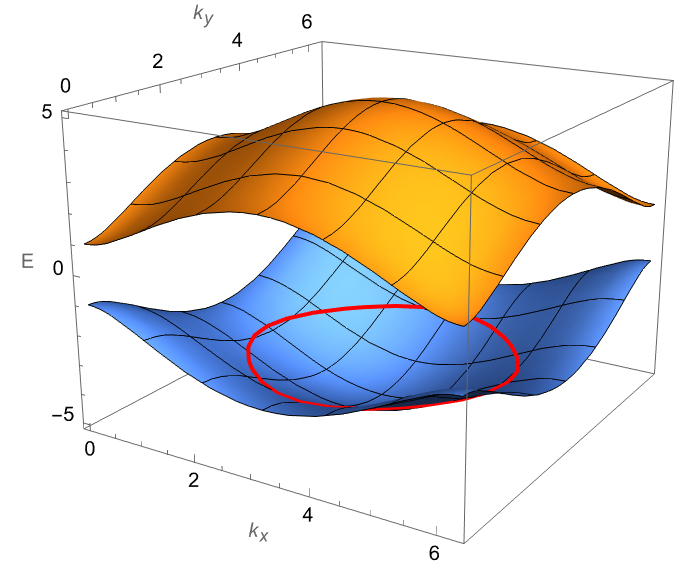
Figure 1: Illustration of the FS from a multi-orbital system, marked by the thick red line, enclosing a Fermi volume and a Berry phase.

Band projection in a weak magnetic field.—Without loss of generality, we consider a 2d multi-orbital metal with a single closed FS, skectched in Fig. 1 in the presence of a magnetic field. $\widehat{H}({\bm{x}},{\bm{p}})=\widehat{H}({\bm{\pi}}={\bm{p}}+{\bm{A}}({\bm{x}}))$, where ${\bm{\pi}}$ is the kinetic momentum following from the Peierls substitution. As a low-energy effective field theory (EFT), we can project the theory onto a single band [42, 43, 44] $\ket{v({\bm{\pi}}})$ and subsequently around the FS. Since $\widehat{H}({\bm{\pi})}$ is treated as a Wigner function instead of a quantum operator, the proper multiplication operator is $\star$ (which satisfies associativity), i.e., the energy eigenstate is given by $\widehat{H}\star\ket{v}=\ket{v}\star\epsilon$, with $\bra{v}\star\ket{v}=1$. The effective action is

$$S_{\rm eff}=\int_{t,{\bm{x}},{\bm{p}}}\bra{v}\star\left(\widehat{f}_{0}\star\widehat{U}^{-1}\star{i}\partial_{t}\widehat{U}-\widehat{f}\star\widehat{H}\right)\star\ket{v}.$$ (3)

Here $\bra{v_{{\bm{\pi}}}}\star\widehat{f}_{0}({{\bm{\pi}}})=f_{0}({{\bm{\pi}}})\star\bra{v_{{{\bm{\pi}}}}}$, where $f_{0}({{\bm{\pi}}})=\theta(\epsilon_{F}-\epsilon({\bm{\pi}}))$ and the low-energy fluctuations are restricted to intra-band ones: $\bra{u}\star\widehat{U}\star\ket{v}=U\delta_{uv}$ [37].

As pointed out in Ref. [24], it is convenient to work in the $({\bm{R}},{\bm{\pi}})$ coordinates of the phase space, where ${\bm{R}}=(x-\pi_{y}/B,y+\pi_{x}/B)$ is the guiding center, as the theory is ${\bm{R}}$-independent due to magnetic translation symmetry. In this situation, the Moyal product simplifies to $\star=\exp[-{i}(B/2){\overleftarrow{\partial_{{\bm{\pi}}}}\times\overrightarrow{\partial_{{{\bm{\pi}}}}}}]$ [24]. Noting that $\ket{v}$ is not the eigenstate of $H$ via matrix multiplication, let us assume instead $H\ket{v_{0}}=\epsilon_{0}\ket{v_{0}}$, where $\innerproduct{v_{0}}{v_{0}}=1$. We can expand $\ket{v}$ as $\ket{v_{0}}+\ket{\delta v}+\mathcal{O}(B^{2})$. We have

$$1 =\bra{v}\star\ket{v}\approx\bra{v_{0}}\star\ket{v_{0}}+2\real\innerproduct{v_{0}}{\delta v}+\mathcal{O}(B^{2})$$

$$=1-B\Omega/2+2\real\innerproduct{v_{0}}{\delta v}+\mathcal{O}(B^{2}),$$

where $\Omega({\bm{\pi}})={i}\bra{v_{0}}{\overleftarrow{\partial_{{{\bm{\pi}}}}}\times\overrightarrow{\partial_{{{{\bm{\pi}}}}}}}\ket{v_{0}}$ is the Berry curvature. We see that $\real\innerproduct{v_{0}}{\delta v}={B\Omega}/4+\mathcal{O}(B^{2}).$ Knowing the expansion of $\ket{v}$, we can then expand the projection of $\widehat{H}$, up to $\mathcal{O}(B^{2})$ corrections,

$$\!\!\!\!\!\!\!\bra{v}\star\widehat{H}({{\bm{\pi}}})\star\ket{v}=2\real\bra{v_{0}}{H}\ket{\delta v}+\bra{v_{0}}\star H\star\ket{v_{0}}$$

$$= \epsilon_{0}(\pi_{x}-B\mathcal{A}_{y},\pi_{y}+B\mathcal{A}_{x})-\mathcal{M}(\pi_{x},\pi_{y})B.$$ (4)

In the weak field limit, the cyclotron frequency $\omega_{c}=Bv_{F}/k_{F}$ is the smallest scale, and $\mathcal{O}(B^{2})$ terms are suppressed by Fermi energy or band gap, and can be safely neglected (which we do hereafter). Here $\mathcal{M}({\bm{\pi}})=-\frac{i}{2}\bra{\nabla_{{\bm{\pi}}}v_{0}}\left[H({\bm{\pi}})-\epsilon({\bm{\pi}})\right]\times\ket{\nabla_{{\bm{\pi}}}v_{0}}$ is the spontaneous orbital magnetic moment, first obtained using semiclassical wave packets [6], and $\bm{\mathcal{A}}({{\bm{\pi}}})={i}\bra{v}\partial_{{{\bm{\pi}}}}\ket{v}$ is the Berry connection. We can thus define the modified kinetic momentum as

$$k_{x,y}\equiv\pi_{x,y}\mp B\mathcal{A}_{y,x},$$ (5)

and the effects of Berry curvature enters through a Jacobian $J=1+B\Omega$ present both in the integration measure and in the Moyal product. Note that while it is tempting to treat $\bm{A}(\bm{x})$ and $\bm{\mathcal{A}}(\bm{p})$ as components of phase-space gauge fields, a direct minimal coupling procedure $({\bm{x}},{\bm{p}})\to({\bm{x}}-\bm{\mathcal{A}},{\bm{p}}+\bm{A})$ is not correct (see [37] for the complete analysis).

After the band projection, the action becomes

$$S=\int_{t,{\bm{R}},{\bm{k}}}(1+B\Omega)\left[f_{0}({\bm{k}})U^{-1}\star{i}\partial_{t}U-f\star\epsilon({\bm{k}})\right],$$ (6)

where $\star=\exp[-{i}B{\overleftarrow{\partial_{\bm{k}}}\times\overrightarrow{\partial_{{\bm{k}}}}}/2(1+B\Omega)]$ in the new coordinates, and the effective dispersion is given by

$$\epsilon({\bm{k}})=\epsilon_{0}({\bm{k}})-\mathcal{M}({\bm{k}})B.$$ (7)

The action (6) agrees with a recent effective field theory phenomenologically obtained from single-particle symplectic mechanics [35]. However, the orbital moment contributes a “Zeeman energy” $-\mathcal{M}({\bm{k}})B$ to the dispersion, which cannot be obtained using the methods there, and has to be assumed to be implicit in $\epsilon({\bm{k}})$. Notably, the saddle point of this action yields $\partial_{t}f({\bm{R}},{\bm{k}},t)=\{f({\bm{R}},{\bm{k}},t),\epsilon({\bm{k}})\}_{\rm M}$, where $\{F,G\}_{\rm M}\equiv-{i}(F\star G-G\star F)$ is the Moyal bracket [40, 24, 41] and can be approximated by the Poisson bracket $\{F,G\}=-{B\partial_{{\bm{k}}}F\times\partial_{{\bm{k}}}G}/{(1+B\Omega({\bm{k}}))}$; indeed, the corrections due to Moyal product comes at $\mathcal{O}(B^{3})$, an even higher order than the Berry curvature effcts. Going back to $({\bm{x}},{\bm{k}})$ coordinates (by the chain rule), we have for $f({\bm{x}},{\bm{k}},t)$

$$\partial_{t}f=\frac{-\bm{v}({\bm{k}})\cdot\partial_{{\bm{x}}}f-B\bm{v}({\bm{k}})\times\partial_{{\bm{k}}}f}{1+B\Omega({\bm{k}}^{\prime})},$$ (8)

where $\bm{v}=\nabla_{{\bm{k}}}\epsilon$. This is precisely the collisionless Boltzmann equation in the presence of Berry curvature and magnetic field. The $1+B\Omega$ factor was first obtained from wave packets [45], and has been shown to follow from band projection [46, 47, 43, 42], although as can be seen in [37], our derivation using $({\bm{R}},{\bm{k}})$ coordinates is significantly more straightforward.

The phase-space field can be expressed as $U({\bm{R}},{\bm{k}})=\exp({i}\phi({\bm{R}},{\bm{k}}))$, where $\phi\simeq\phi+2\pi$ is a real compact field. We expand the effective action up to quadratic order in $\phi$, and drop terms that are also higher-order in $B$. When $\phi$ is single-valued, the quadratic action in the weak field limit reads

$$S^{(2)}=\int\frac{d{\bm{R}}d{\bm{k}}}{8\pi^{2}}(1+B\Omega)\{\phi,f_{0}({\bm{k}})\}\left(\dot{\phi}-\{\epsilon({\bm{k}}),\phi\}\right).$$ (9)

Further, as shown in Ref. [24], due to magnetic translation symmetry, the integral over noncommutative (phase-space) coordinates ${\bm{R}}$ can be converted to a sum over $N_{\phi}$ magnetic Bloch states in the magnetic Brillouin zone (mBZ), where $N_{\phi}=BL^{2}/2\pi$ is the Landau level degeneracy: we have

$$\int\frac{d{\bm{R}}}{2\pi B^{-1}}...=\Tr_{\widehat{\bm{R}}}...=\sum_{\bm{K}_{i}\in\rm mBZ}\bra{\bm{K}_{i}}...\ket{\bm{K}_{i}}.$$

In addition, it suffices [24] to only include in the path integral $\phi(\widehat{\bm{R}},{\bm{k}})$ that are invariant under magnetic translation, i.e., $\bra{\bm{K}_{i}}\phi(\widehat{\bm{R}},{\bm{k}})\ket{\bm{K}_{j}}=\phi_{i}({\bm{k}})\delta_{ij}$.

Let us assume the FS is isotropic, and show the analysis for anisotropic FS’s in [37]. In terms of $\phi_{i}({\bm{k}})$’s, the effective action is given by $S_{\rm eff}=\sum_{i=1}^{N_{\phi}}(S_{\rm cb}+S_{\rm w})$, with

$$S_{\rm cb}= \int\frac{dtd\theta}{4\pi}\partial_{\theta}\phi_{i}\left(\dot{\phi}_{i}-\frac{\omega_{c}}{1+B\Omega_{\theta}}\partial_{\theta}\phi_{i}\right)$$ (10)

$$S_{\rm w}= \int\frac{dtd^{2}k}{2\pi}f_{0}({\bm{k}})\left[-\frac{1+B\Omega}{B}\dot{\phi}_{i}+\frac{1}{2}(\partial_{{\bm{k}}}\times\partial_{{\bm{k}}}\phi_{i})\dot{\phi_{i}}\right],$$

where the cyclotron frequency $\omega_{c}=Bv_{F}/k_{F}$ and $\Omega_{\theta}=\partial_{{\bm{k}}}\times\bm{\mathcal{A}}|_{k=k_{F}}$ are taken on the FS. The $S_{\rm cb}[\phi_{i}(\theta,t)]$ term directly follows from Eq. (9), where $\theta$ parametrizes the tangential direction along the Fermi surface. It describes a chiral boson propagating in 1d momentum space [48]. The additional $S_{\rm w}[\phi_{i}({\bm{k}},t)]$ term previously neglected [24] is nonzero only when $\phi_{i}$ contains winding configurations, and is topological (depending only on the winding numbers). As is well-known [49], topological terms do not enter the equation of motion (8), but they do affect the quantization of theory.

Mode expansion and quantization.—We perform a mode expansion for the compact field $\phi_{i}$ as

$$\phi_{i}(\theta)=q_{i}+p_{i}\theta+\sum_{n\neq 0}\frac{a_{i,n}}{\sqrt{|n|}}e^{{i}n\theta},~\theta\in[-\pi,\pi),$$

where $q_{i}\simeq q_{i}+2\pi$, and $p_{i}$ is a winding number. For $p_{i}\neq 0$, the $U_{i}={e}^{{i}\phi_{i}({\bm{k}})}$ field has a singular (vortex) configuration in ${\bm{k}}$, which requires an extension of the coherent states $\ket{\mathcal{U}}$ in the path integral [24]. The physical meaning of $p_{i}$ is the extra occupation number at a given $\bm{K}_{i}$. Indeed, from

$$\!\!\!\!\!\delta f_{i}=\int_{\bm{k}}(1+B\Omega)\left({e}^{{i}\phi_{i}}\star f_{0}\star{e}^{-{i}\phi_{i}}-f_{0}\right)=-\int_{\theta}\frac{\partial_{\theta}\phi_{i}}{2\pi}$$ (11)

we see that adding $p_{i}\neq 0$ configurations for each $\bm{K}_{i}$ ensures the system to be in a grand canonical ensemble (as it should for fixed $\mu$).

To quantize $S_{\rm w}$ we need to extend the mode expansion into the Fermi sea, but since the term is topological, the specific form of extension does not matter [24]. The action splits into a Fock sector and a zero-mode sector, $S_{\rm cb}[\phi]+S_{\rm w}[\phi]=S_{\rm Fock}\left[a_{n}\right]+S_{\rm zero}[p,q]$. As shown in Ref. [24], $S_{\rm Fock}$ is responsible for specific heat and Landau diamagnetism for $T\gg\omega_{c}$, which we will not discuss here.

The zero-mode action can be written as

$$\!\!\!\!\!S_{\rm zero}[p,q]=\int dt\left[\left(-\frac{\mathcal{A}_{\rm FS}}{2\pi B}-\frac{\gamma}{2\pi}\right)\dot{q}+p\dot{q}-\frac{\bar{\omega}_{c}}{2}p^{2}\right],$$ (12)

where $\gamma=\int_{\bm{k}}f_{0}({\bm{k}})\Omega({\bm{k}})$ is the Berry phase around the FS, and the effective cyclotron frequency [45] for a generic FS is [37]

$$\bar{\omega}_{c}(B,\Omega)=\frac{B}{2\pi g(\epsilon_{F},B)}\left\langle\frac{1}{1+B\Omega_{\theta}}\right\rangle_{\rm FS},$$ (13)

where $g(\epsilon_{F},B)$ is the density of states obtained from (7), and $\langle...\rangle_{\rm FS}$ denotes an average over the FS for anisotropic cases.

Interestingly, the action (12) exactly maps to a single-particle quantum mechanical problem of a charged particle moving on a ring with a flux through it, where the first term is a topological $\theta$-term [49]. At a finie temperature $1/\beta$, the partition function is

$$Z_{\rm zero}=\sum_{p^{\prime}\in\mathbb{Z}}\exp[-\frac{\beta\bar{\omega}_{c}}{2}\left(p^{\prime}+\frac{\mathcal{A}_{\rm FS}}{2\pi B}+\frac{\gamma}{2\pi}\right)^{2}].$$ (14)

We clearly see that this result is periodic in ${\mathcal{A}_{\rm FS}}/{B}+\gamma\mod 2\pi$ at low-temperatures, and becomes non-oscillatory at $T\gg\bar{\omega}_{c}$ when the summation can be replaced by integral. This is precisely the origin of dHvA.

Modified Lifshitz-Kosevich formula.—The oscialltion of orbital magnetization in an external field can be obtained by evaluating the free energy of the zero-mode partition function, $F_{\rm osc}=-T\log Z_{\rm zero}$. Using the Poisson resummation formula,

$$\!\!\!\!F_{\rm osc}= -N_{\phi}T\log\left[1+2\sum_{n=1}^{\infty}\cos\left(n\Delta\right)q^{n^{2}}\right]$$

$$= -2N_{\phi}T\real\sum_{m=1}^{\infty}\log(1+q^{2m-1}{e}^{{i}\Delta})+\textrm{non-osc.}$$

where $q=\exp(-2\pi^{2}T/\bar{\omega}_{c})$ and $\Delta=\mathcal{A}_{\rm FS}/B+\gamma$. In the first line, the argument of the log is nothing but the Jacobi theta function $\theta_{3}(\Delta/2,q)$, which also admits a product form, which we used in the second line [50, 37]. Expanding the log in the second line and performing the summation over $m$, we obtain [37]

$$F_{\rm osc} =N_{\phi}T\sum_{k=1}^{\infty}A_{k}\cos\left[k\left(\frac{\mathcal{A}_{\rm FS}}{B}+\gamma\right)\right],$$

$$\textrm{where }A_{k}=\frac{(-)^{k}}{k\sinh\left(2\pi^{2}kT/\bar{\omega}_{c}\right)}.$$ (15)

We emphasize that the periodicity is rooted in the topological $\theta$-term in (12), and survives even for interacting systems such as Fermi liquids and non-Fermi liquids [30]. While the Luttinger theorem [51, 52, 53] ensures the physical meaning of $\mathcal{A}_{\rm FS}$, a natural question is that of $\gamma$ beyond single-particle physics.

$\gamma$ and Anomalous Hall Conductance.—The canonical quantization of $S_{\rm cb}+S_{\rm w}$, leads to the Kac-Moody algebra [54, 53, 24]

$$[\hat{n}_{i}(\theta),\hat{n}_{i}(\theta^{\prime})]=\frac{-{i}}{2\pi}\delta^{\prime}(\theta-\theta^{\prime}),$$ (16)

where $n_{i}(\theta)\equiv-\partial_{\theta}\phi_{i}(\theta)/2\pi$ is the density of electrons with magnetic momentum $\bm{K}_{i}$, as can be seen from Eq. (11).

For a system without Berry phases, This algebra was used [53] to obtain a nonperturbative derivation of the Luttinger’s theorem. In our context, let’s set $N_{\phi}=1$ and consider the braiding algebra between “translation” operators generated by kinetic momentum ${\bm{\pi}}$: $\hat{\mathbb{T}}_{x,y}=\exp({i}\sum_{{\bm{\pi}}}\hat{N}_{{\bm{\pi}}}\pi_{x,y})$, where $\hat{N}_{{\bm{\pi}}}$ is the particle number operator and we set lattice constant $a=1$. From basic quantum mechanics, $\hat{\mathbb{T}}_{x}\hat{\mathbb{T}}_{y}\hat{\mathbb{T}}_{x}^{-1}\hat{\mathbb{T}}_{y}^{-1}={e}^{2\pi{i}\nu}$ [37, 53], where $\nu$ is the filling fraction of the band. In the low-energy limit, the lattice translation operators become $\hat{\mathbb{T}}_{x,y}\sim\exp{{i}\int_{\theta}\hat{n}(\theta)\left[k_{F;x,y}(\theta)\pm B\mathcal{A}_{y,x}(\theta)\right]},$ where $k_{F;x,y}$ are the components of the Fermi momentum and we have used (5). Together with (16), the same braiding algebra evaluates to [37]

$$\hat{\mathbb{T}}_{x}\hat{\mathbb{T}}_{y}\hat{\mathbb{T}}_{x}^{-1}\hat{\mathbb{T}}_{y}^{-1}=\exp[{i}\frac{\mathcal{A}_{\rm FS}}{2\pi}+{i}\frac{B\gamma}{2\pi}],$$ (17)

where $\gamma\equiv\oint\bm{\mathcal{A}}\cdot{d}{\bm{k}}$ is the same as that in (12) via Stokes theorem. Relating the right band sides, we get $4\pi^{2}\nu=\mathcal{A}_{\rm FS}+B\gamma$. The first term corresponds to the Luttinger theorem [53], while the second term describes the Streda formula $\nu=\sigma_{xy}^{H}B$ relating the linear charge response to a $B$ field to the static (anomalous) Hall conductance [55, 35]. We have (in units of $e^{2}/\hbar$)

$$\sigma_{xy}^{H}(q\to 0,\omega=0)=\frac{\gamma}{4\pi^{2}}.$$ (18)

This result was long known for free fermions [45, 56], and we emphasize that our derivation only takes input from low energies  and applies even for interacting systems (see also Ref. [58]). In particular, it is well-known that the commutation relation (16) is unaffected by interaction effects [54, 53, 30]. For Fermi liquids, $\gamma$ can be understood as the Berry phase of the quasiparticle.  Beyond, the relation (18) holds even for e.g., non-Fermi liquids.

Discussion.—The key result of this work, Eq. (15), takes a similar form of the Lifshitz-Kosevich formula [18], with two important differences. First, the phase shift $\gamma$ in the quantum oscillations goes beyond the single-particle Berry phase for free fermions, and by (18) should precisely match the static anomalous Hall conductance, which can be extracted from spatially-resolved transport [60]. Second, the Berry curvature on the FS leads to a renormalized cyclotron frequency $\bar{\omega}_{c}(B)$ in (13) that is nonlinear in $B$ (due to both Berry phase and the magnetic moment), which alters the finite-temperature suppression of the dHvA amplitudes. For $T\geq\bar{\omega}_{c}$, from (13, 15) there exists an additional $\lambda_{2}$ term in $A_{k}$:

$$A_{k}\propto\exp(-\frac{\lambda_{1}T}{B})\exp(\lambda_{2}T),$$ (19)

which can be directly tested in 2d materials with strong Berry curvature on the Fermi surface. We note that unlike the phase shift, the amplitude $A_{k}$ in general receives additional corrections from interaction effects, which we will address in an upcoming work [61]. Finally, it would be interesting to extend our results to 3d systems.

oneΔSupplemental Material to “Berry Phase and Quantum Oscillation from Multi-orbital Coadjoint-orbit Bosonization” January 7, 2025

oneΔ

I Band projection procedure for general phase space coordinates

In this section, we generalize the band projection procedure discussed in the main text (Eq. (3)) to a general set of phase space coordinates. We show that while the action derived in Eq. (6) of the main text remains the same using different choices of phase space coordinates, proper coordinates can be chosen to simplify the calculation. Furthermore, the procedure can be readily applied to electromagnetic responses, and to the leading order in the gradient expansion, the electromagnetic responses only depend on the Berry curvature.

The Moyal product in a set of phase space coordinates $\{\xi^{i}\}$ with $i=1,2,..,2d$ reads

$$F\star G=F\exp{\frac{i\hbar}{2}\mathbb{\Omega}^{ij}_{\xi}\overleftarrow{\partial}_{\xi^{i}}\overrightarrow{\partial}_{\xi^{j}}}.$$ (S1)

where $\mathbb{\Omega}^{ij}_{\xi}$ is the symplectic 2-form for the phase space coordinates ${\bm{\xi}}$. One may express Eq. (S1) as a gradient expansion with terms that are increasingly irrelevant for the low-energy effective field theory (EFT). To keep track of the order in the gradient expansion, we have introduced a dimensionless parameter $\hbar$ in Eq. (S1), whereas the Plank constant and unit charge is set to one. We then have $B=\ell_{B}^{-2}$, where $\ell_{B}$ is the magnetic length. Below, we consider $d=2$, and define ${\bm{\pi}}={\bm{p}}+{\bm{A}}$, ${\bm{R}}=\ell_{B}^{2}({\bm{p}}-{\bm{A}})\times\hat{z}$. For coordinates $\{x,y,p_{x},p_{y}\}$, $\{x,y,\pi_{x},\pi_{y}\}$ and $\{R_{x},R_{y},\pi_{x},\pi_{y}\}$, $\mathbb{\Omega}$ reads, respectively,

$$\mathbb{\Omega}_{{\bm{x}},{\bm{p}}}=\begin{pmatrix}0&0&1&0\\ 0&0&0&1\\ -1&0&0&0\\ 0&-1&0&0\\ \end{pmatrix},\quad\mathbb{\Omega}_{{{\bm{x}}},{{\bm{\pi}}}}=\begin{pmatrix}0&0&1&0\\ 0&0&0&1\\ -1&0&0&-B\\ 0&-1&B&0\\ \end{pmatrix},\quad\mathbb{\Omega}_{{\bm{R}},{\bm{\pi}}}=\begin{pmatrix}0&1/B&0&0\\ -1/B&0&0&0\\ 0&0&0&-B\\ 0&0&B&0\\ \end{pmatrix}$$ (S2)

Note that Eq. (S1) is exact for $\{{\bm{x}},{\bm{p}}\}$, $\{{\bm{x}},{\bm{\pi}}\}$, and $\{{\bm{R}},{\bm{\pi}}\}$ coordinates, but its validity to all orders in the Moyal product has not been studied well for generalized phase space coordinates projected to a single band, like Eq. (S19) we define below.

The multi-orbital coadjoint-orbit action reads

$$S=\int{d}t\frac{{d}{\bm{\xi}}}{(2\pi)^{2}}\Tr\left[\widehat{f}_{0}({\bm{\xi}})\star\widehat{U}^{-1}({\bm{\xi}},t)\star{i}\partial_{t}\widehat{U}({\bm{\xi}},t)-\widehat{f}({\bm{\xi}},t)\star\widehat{H}({\bm{\xi}})\right]$$ (S3)

where we have used $\sqrt{\mathrm{Det}\mathbb{\Omega}}=1$ from Eq. (S2). Here, we take Eq. (S1) and (S3) as the starting point, and derive the effective action projected onto a band with a Fermi surface for a generic single particle Hamiltonian $\widehat{H}({\bm{\xi}})$. In particular, for a multi-orbital system that couples to external electromagnetic fields, we choose the gauge such that $\widehat{H}({\bm{\xi}})=\widehat{H}_{0}({\bm{p}}+{\bm{A}})+A_{0}({\bm{x}})=\widehat{H}_{0}({\bm{k}})+A_{0}({\bm{x}})$, where ${\bm{\nabla}}\times{\bm{A}}=B\hat{z},-{\bm{\nabla}}A_{0}={\bm{E}}$.

I.1 Star diagonalization

As a notational convention, we use $\widehat{V}$ to denote a matrix $V$ in orbital basis. Under the Moyal star product, we define a unitary transformation $\widehat{V}({\bm{\xi}})\star\widehat{V}({\bm{\xi}})^{\dagger}=\widehat{V}({\bm{\xi}})^{\dagger}\star\widehat{V}({\bm{\xi}})=1$ such that a Hermitian matrix $\widehat{H}({\bm{\xi}})$ is star-diagoanlized [62, 44], defined as $\widehat{\mathcal{E}}=\widehat{V}\star\widehat{H}\star\widehat{V}^{\dagger}$. As the Moyal product is associative, the coadjoint orbit action Eq. (S4) can be written as

$$S=\int{d}t\frac{{d}{\bm{\xi}}}{(2\pi)^{2}}\Tr\left[\widehat{f}_{0,d}({\bm{\xi}})\star\widehat{U}_{v}^{-1}({\bm{\xi}},t)\star{i}\partial_{t}\widehat{U}_{v}({\bm{\xi}},t)-\widehat{f}_{v}({\bm{\xi}},t)\star\widehat{\mathcal{E}}({\bm{\xi}})\right]$$ (S4)

where $\widehat{f}_{0,d}({\bm{\xi}})=\widehat{V}\star\widehat{f}_{0}({\bm{\xi}})\star\widehat{V}^{\dagger}$, $\widehat{U}_{v}({\bm{\xi}})=\widehat{V}\star\widehat{U}({\bm{\xi}})\star\widehat{V}^{\dagger}$. Note that while $\widehat{f}_{0,d}$ and $\widehat{\mathcal{E}}$ are diagonal (defined as the band basis), $\widehat{U}_{v}$ and $\widehat{f}_{v}$ are not diagonal in general. However, the off-diagonal terms should be fast oscillating for band gap much greater than the EFT cutoff, and will be ignored hereafter. Projecting the action to the band (indexed by “$a$”) at the chemical potential, the action reads

$$S_{a}=\int{d}t\frac{{d}{\bm{\xi}}}{(2\pi)^{2}}\left[f_{0,a}({\bm{\xi}})\star U_{v,a}^{-1}({\bm{\xi}},t)\star{i}\partial_{t}U_{v,a}({\bm{\xi}},t)-U_{v,a}({\bm{\xi}},t)\star f_{v,a}({\bm{\xi}},t)\star U^{-1}_{v,a}({\bm{\xi}},t)\star{\mathcal{E}}_{a}({\bm{\xi}})\right]$$ (S5)

where $f_{0,a},U_{v,a},f_{v,a}$ and ${\mathcal{E}}_{a}$ are the diagonal “$aa$” elements of the corresponding matrices in the band basis. In the $({\bm{R}},{\bm{\pi}})$ basis, and for Hamiltonian $\widehat{H}({\bm{\xi}})=\widehat{H}({{\bm{\pi}}})$, we can equate the expressions in the main text with expressions here by $f_{0}({\bm{\pi}})={f}_{0,a}$, $U={U}_{v,a}$, $\epsilon({\bm{\pi}})={\mathcal{E}}_{a}$, and Eq. (S5) can be equivalently expressed as Eq. (3) in the main text. At first sight, it is equivalent to the coadjoint orbit action for a single band Hamiltonian. However, note that ${\mathcal{E}}_{a}({\bm{\xi}})$ is obtained from the star diagonalization of $\widehat{H}$, which is different from the “band dispersion” obtained via the usual matrix diagonalization. To relate the two, define a unitary transformation $\widehat{V}_{0}$ that diagonalize $\widehat{H}$, i.e. $\widehat{V}_{0}\widehat{H}\widehat{V}_{0}^{\dagger}=\widehat{\mathcal{E}}_{0}$, such that

$$\widehat{V}=(1+\widehat{V}_{1}+\widehat{V}_{2}+..)\widehat{V}_{0}\textrm{, where {\hbox{\widehat{V}_n \sim\mathcal{O}(\hbar^n)}}.}$$ (S6)

Similarly, $\widehat{\mathcal{E}}=\widehat{\mathcal{E}}_{0}+\sum_{n=1}^{\infty}\widehat{\mathcal{E}}_{n}$ where $\widehat{\mathcal{E}}_{n}\sim\mathcal{O}(\hbar^{n})$. As $\widehat{V}_{0}$ and $\widehat{\mathcal{E}}_{0}$ encodes all information in $\widehat{H}$, $\widehat{V}_{n}$ and $\widehat{\mathcal{E}}_{n}$ ($n\geq 1$) can be determined order by order in terms of $\widehat{V}_{0}$ and $\widehat{\mathcal{E}}_{0}$ given the symplectic 2-form $\mathbb{\Omega}^{ij}$.

This procedure has been introduced and applied in earlier studies [62] in terms of $\{{\bm{x}},{\bm{p}}\}$ coordinates. Below, we apply the procedure for a set of generic phase space coordinates $\{{\bm{\xi}}\}$ and obtain the leading order terms in the gradient expansion, i.e. $\widehat{V}_{1}$ and $\widehat{\mathcal{E}}_{1}$.

Using $\widehat{V}\star\widehat{V}^{\dagger}=\widehat{V}^{\dagger}\star\widehat{V}=1$ and $\widehat{V}_{0}\widehat{V}_{0}^{\dagger}=\widehat{V}_{0}\widehat{V}_{0}^{\dagger}=1$, we find

$$\widehat{V}_{1}+\widehat{V}_{1}^{\dagger}+\frac{i\hbar}{2}\mathbb{\Omega}^{ij}\widehat{\mathcal{A}}_{i}\widehat{\mathcal{A}}_{j}=0$$ (S7)

where

$$\widehat{\mathcal{A}}_{i}=i\widehat{V}_{0}\partial_{\xi^{i}}\widehat{V}_{0}^{\dagger}=\widehat{\mathcal{A}}_{i}^{\dagger}$$ (S8)

is the non-Abelian phase-space Berry connection, satisfying $(\partial_{i}\widehat{\mathcal{A}}_{j})-(\partial_{j}\widehat{\mathcal{A}}_{i})=i[\widehat{\mathcal{A}}_{i},\widehat{\mathcal{A}}_{j}]$. The last term in (S7) is Hermitian, and thus $\widehat{V}_{1}$ can be expressed via Hermitian and anti-Hermitian parts as

$$\widehat{V}_{1}=-\frac{i\hbar}{4}\mathbb{\Omega}^{ij}\widehat{\mathcal{A}}_{i}\widehat{\mathcal{A}}_{j}+\widehat{\mathcal{Y}}_{1},\text{ where }\widehat{\mathcal{Y}}_{1}^{\dagger}=-\widehat{\mathcal{Y}}_{1}.$$ (S9)

The correction to the energy eigenvalue, $\widehat{\mathcal{E}}_{1}$ can be obtained by expanding $\widehat{\mathcal{E}}=\widehat{V}\star\widehat{H}\star\widehat{V}^{\dagger}$ to the leading order in $\hbar$. We have

$$\widehat{\mathcal{E}}=(1+\widehat{V}_{1})\widehat{V}_{0}\left(1+\frac{i\hbar}{2}\mathbb{\Omega}^{ij}\overleftarrow{\partial}_{i}\overrightarrow{\partial}_{j}\right)\left[\widehat{H}\left(1+\frac{i\hbar}{2}\mathbb{\Omega}^{ij}\overleftarrow{\partial}_{i}\overrightarrow{\partial}_{j}\right)\widehat{V}_{0}^{\dagger}(1+\widehat{V}_{1}^{\dagger})\right]+\mathcal{O}(\hbar^{2})$$ (S10)

where we have made use of the associativity of the Moyal product. The left/right arrowed derivatives act on all terms to their left/right until stopped by an unpaired left/right square bracket. At order $\hbar$, we find

$$\widehat{\mathcal{E}}_{1}= \widehat{V}_{1}\widehat{\mathcal{E}}_{0}+\widehat{\mathcal{E}}_{0}\widehat{V}_{1}^{\dagger}+\frac{i\hbar}{2}\mathbb{\Omega}^{ij}\left(i\widehat{\mathcal{A}}_{i}\widehat{V}_{0}(\partial_{j}\widehat{H})\widehat{V}_{0}^{\dagger}+\widehat{\mathcal{A}}_{i}\widehat{\mathcal{E}}_{0}\widehat{\mathcal{A}}_{j}-i\widehat{V}_{0}(\partial_{i}\widehat{H})\widehat{V}_{0}^{\dagger}\widehat{\mathcal{A}}_{j}\right)$$

$$= \widehat{V}_{1}\widehat{\mathcal{E}}_{0}+\widehat{\mathcal{E}}_{0}\widehat{V}_{1}^{\dagger}-\frac{\hbar}{2}\mathbb{\Omega}^{ij}\{\widehat{\mathcal{A}}_{i},(\partial_{j}\widehat{\mathcal{E}}_{0})\}_{+}+\frac{i\hbar}{2}\mathbb{\Omega}^{ij}\{\widehat{\mathcal{A}}_{i},\left[\widehat{\mathcal{A}}_{j},\widehat{\mathcal{E}}_{0}\right]\}_{+}+\frac{i\hbar}{2}\mathbb{\Omega}^{ij}\widehat{\mathcal{A}}_{i}\widehat{\mathcal{E}}_{0}\widehat{\mathcal{A}}_{j}$$

$$= \left[\mathcal{Y}_{1},\widehat{\mathcal{E}}_{0}\right]-\frac{\hbar}{2}\mathbb{\Omega}^{ij}\{\widehat{\mathcal{A}}_{i},(\partial_{j}\widehat{\mathcal{E}}_{0})\}_{+}+\frac{i\hbar}{4}\mathbb{\Omega}^{ij}\left(\widehat{\mathcal{A}}_{i}\widehat{\mathcal{A}}_{j}\widehat{\mathcal{E}}_{0}+\widehat{\mathcal{E}}_{0}\widehat{\mathcal{A}}_{i}\widehat{\mathcal{A}}_{j}-2\widehat{\mathcal{A}}_{i}\widehat{\mathcal{E}}_{0}\widehat{\mathcal{A}}_{j}\right)$$ (S11)

From the first to the second line, we have used $\widehat{V}_{0}(\partial_{i}\widehat{H})\widehat{V}_{0}^{\dagger}=\partial_{i}\widehat{\mathcal{E}}_{0}-i\left[\widehat{\mathcal{A}}_{i},\widehat{\mathcal{E}}_{0}\right]$. From the second to the third line, we have used Eq. (S9). The dispersion projected to band “$a$” can be read off from the corresponding diagonal element. Noticing that $\left[\widehat{\mathcal{Y}}_{1},\widehat{\mathcal{E}}_{0}\right]$ is an antisymmetric matrix, we have

$${\mathcal{E}}_{a}= {\mathcal{E}}_{0,a}-\hbar\mathbb{\Omega}^{ij}\widehat{\mathcal{A}}_{i}^{aa}(\partial_{j}{\mathcal{E}}_{0,a})+\frac{i}{4}\hbar\mathbb{\Omega}^{ij}\left(\widehat{\mathcal{A}}_{i}\widehat{\mathcal{A}}_{j}\widehat{\mathcal{E}}_{0}+\widehat{\mathcal{E}}_{0}\widehat{\mathcal{A}}_{i}\widehat{\mathcal{A}}_{j}-2\widehat{\mathcal{A}}_{i}\widehat{\mathcal{E}}_{0}\widehat{\mathcal{A}}_{j}\right)^{aa}+\mathcal{O}(\hbar^{2})$$

$$= {\mathcal{E}}_{0,a}-\hbar\mathbb{\Omega}^{ij}\widehat{\mathcal{A}}_{i}^{aa}(\partial_{j}{\mathcal{E}}_{0,a})-\frac{i}{2}\hbar\mathbb{\Omega}^{ij}\left[-\left(\widehat{\mathcal{A}}_{i}\widehat{\mathcal{E}}_{0}\widehat{\mathcal{A}}_{j}\right)^{aa}+i\partial_{i}\widehat{\mathcal{A}}^{aa}_{j}{\mathcal{E}}_{0,a}\right]+\mathcal{O}(\hbar^{2})$$

$$= {\mathcal{E}}_{0,a}(\xi^{i}+\hbar\mathbb{\Omega}^{ij}{\mathcal{A}}_{j})-\frac{i}{2}\hbar\mathbb{\Omega}^{ij}\bra{\partial_{i}v_{a}}(\widehat{H}-{\mathcal{E}}_{0,a})\ket{\partial_{j}v_{a}}+\mathcal{O}(\hbar^{2})$$ (S12)

To be concise, we have defined in the last line the intra-band (Abelian) phase-space Berry connection as $\mathcal{A}_{i}=\widehat{\mathcal{A}}^{aa}_{i}$ and $\bm{\mathcal{A}}=\widehat{{\bm{\mathcal{A}}}}^{aa}$. Eq. (S12) is the main result of this subsection. It shows that there are two contributions to the dispersion at $\hbar$ order. The second term on the RHS of the first line shift the coordinate $\xi^{i}$, the third term modifies the spectrum. Below, we discuss two applications. First, we consider coupling the theory to an external perpendicular magnetic field. Second, we consider the effect of both magnetic and electric field.

I.2 Coadjoint orbit EFT in an external magnetic field

In $\{{\bm{x}},{\bm{\pi}}\}$ or $\{{\bm{R}},{\bm{\pi}}\}$ coordinates, the Hamiltonian reads $\widehat{H}({\bm{\xi}})=\widehat{H}({\bm{\pi}}={\bm{p}}+{\bm{A}})$. From Eq. (S2), the modified dispersion up to order $\hbar$ reads

$${\mathcal{E}}_{a}({\bm{\pi}})={\mathcal{E}}_{0,a}(\pi_{x}-\hbar B\mathcal{A}_{\pi_{y}},\pi_{y}+\hbar B\mathcal{A}_{\pi_{x}})+\frac{i\hbar B}{2}\bra{\partial_{{\bm{\pi}}}v_{a}}(\widehat{H}-{\mathcal{E}}_{0,a})\times\ket{\partial_{{\bm{\pi}}}v_{a}}+\mathcal{O}(\hbar^{2}).$$ (S13)

Noting that the $\pi_{x,y}$ component of the phase-space Berry connection is just the momentum-space Berry connection in the main text, this is precisely Eq. (3) we derived in the main text (after setting the expansion parameter $\hbar=1$).

In the $\{{\bm{x}},{\bm{p}}\}$ coordinates, we expect the same result. However, the calculation is more involved. The modified dispersion up to order $\hbar$ reads

$${\mathcal{E}}_{a}({\bm{p}}+{\bm{A}})= {\mathcal{E}}_{0,a}({\bm{p}}-\hbar\bm{\mathcal{\bm{A}}}_{{\bm{x}}}+{\bm{A}}({\bm{x}}+\hbar\bm{\mathcal{\bm{A}}}_{{\bm{p}}}))-\frac{i}{2}\hbar\left\{\sum_{l=x,y}\left[-\left(\widehat{\mathcal{A}}_{{\bm{x}}_{l}}\widehat{\mathcal{E}}_{0}\widehat{\mathcal{A}}_{{\bm{p}}_{l}}\right)^{aa}+i\partial_{{\bm{x}}_{l}}\mathcal{A}_{{\bm{p}}_{l}}{\mathcal{E}}_{0,a}\right]-\left({\bm{x}}\leftrightarrow{\bm{p}}\right)\right\}+\mathcal{O}(\hbar^{2})$$

$$= {\mathcal{E}}_{0,a}({\bm{p}}-\hbar\bm{\mathcal{\bm{A}}}_{{\bm{x}}}-\frac{B}{2}({\bm{x}}+\hbar\bm{\mathcal{\bm{A}}}_{{\bm{p}}})\times\hat{z})-\frac{i}{2}\hbar\left\{\sum_{l=x,y}\left[-\left(\widehat{\mathcal{A}}_{{\bm{x}}_{l}}\widehat{\mathcal{E}}_{0}\widehat{\mathcal{A}}_{{\bm{p}}_{l}}\right)^{aa}+i\partial_{{\bm{x}}_{l}}\mathcal{A}_{{\bm{p}}_{l}}{\mathcal{E}}_{0,a}\right]-\left({\bm{x}}\leftrightarrow{\bm{p}}\right)\right\}+\mathcal{O}(\hbar^{2})$$

$$= {\mathcal{E}}_{0,a}({\bm{p}}+{\bm{A}}-\hbar B\bm{\mathcal{\bm{A}}}_{{\bm{p}}}\times\hat{z})+\frac{i\hbar B}{2}\bra{\partial_{{\bm{p}}}v_{a}}(\widehat{H}-{\mathcal{E}}_{0,a})\times\ket{\partial_{{\bm{p}}}v_{a}}+\mathcal{O}(\hbar^{2})$$ (S14)

By definition,

$$\widehat{\mathcal{A}}_{{\bm{x}}_{l}}= i\widehat{V}_{0}({\bm{p}}+{\bm{A}})\partial_{{\bm{x}}_{l}}\widehat{V}_{0}^{\dagger}({\bm{p}}+{\bm{A}})$$ (S15)

$$\widehat{\mathcal{\bm{A}}}_{{\bm{p}}_{l}}= i\widehat{V}_{0}({\bm{p}}+{\bm{A}})\partial_{{\bm{p}}_{l}}\widehat{V}_{0}^{\dagger}({\bm{p}}+{\bm{A}})=\widehat{\mathcal{\bm{A}}}_{{\bm{\pi}}_{l}},$$ (S16)

To obtain the last line in Eq. (S14), we have used $\widehat{\mathcal{A}}_{{\bm{x}}_{j}}=i\widehat{V}_{0}\partial_{{\bm{x}}_{j}}\widehat{V}_{0}^{\dagger}=i\widehat{V}_{0}\partial_{{\bm{p}}_{i}}\widehat{V}_{0}^{\dagger}|_{{\bm{p}}+{\bm{A}}}\frac{\partial{\bm{A}}_{i}}{\partial{\bm{x}}_{j}}=-\frac{B}{2}\epsilon_{ij}\widehat{\mathcal{A}}_{{\bm{p}}_{i}}=-\frac{B}{2}\epsilon_{ij}\widehat{\mathcal{A}}_{{\bm{\pi}}_{i}}$, and $\partial_{{\bm{x}}_{i}}\widehat{\mathcal{A}}_{{\bm{p}}_{i}}=\partial_{{\bm{p}}_{j}}\widehat{\mathcal{A}}_{{\bm{p}}_{i}}\frac{\partial{\bm{A}}_{j}}{\partial{{\bm{x}}_{i}}}=-\frac{B}{2}\epsilon_{ij}\partial_{{\bm{p}}_{i}}\widehat{\mathcal{A}}_{{\bm{p}}_{j}}=-\frac{B}{2}\epsilon_{ij}\partial_{{\bm{\pi}}_{i}}\widehat{\mathcal{A}}_{{\bm{\pi}}_{j}}$.

It is straightforward to check that Eq. (S13) and (S14) are equivalent up to $\mathcal{O}(\hbar)$. However, from this exercise, we see that in homogeneous magnetic field, the calculation can be done more conveniently in the $\{{\bm{x}},{\bm{\pi}}\}$ or $\{{\bm{R}},{\bm{\pi}}\}$ phase space coordinates as long as the symplectic 2-form is properly chosen as in Eq. (S2).

I.3 Semiclassical Boltzmann equation in external electromagnetic fields

In this subsection, we demonstrate the band projection procedure in the presence of an additional static electric field, which is useful for, e.g., transport. In the presence of both electric and magnetic field, the Hamiltonian in Eq. (S4) reads

$$\widehat{H}({\bm{\xi}})=\widehat{H}_{0}({\bm{\pi}})+A_{0}({\bm{x}})\textrm{, where }{\bm{E}}=-\nabla_{{\bm{x}}}A_{0},\,B\hat{z}=\nabla_{{\bm{x}}}\times{\bm{A}}$$ (S17)

For simplicity, we use the $\{{\bm{x}},{\bm{\pi}}\}$ phase space coordinates. As the potential term $A_{0}({\bm{x}})$ is diagonal in the band basis, the only nonzero phase space Berry connection is $\widehat{\mathcal{A}}_{{\bm{\pi}}}=i\widehat{V}_{0}({\bm{\pi}})\partial_{{\bm{\pi}}}\widehat{V}_{0}^{\dagger}({\bm{\pi}})$, where $\widehat{V}_{0}\widehat{H}_{0}({\bm{\pi}})\widehat{V}_{0}^{\dagger}=\widehat{\mathcal{E}}_{{\rm band},0}$ gives the spectrum in zero magnetic field. Following Eq. (S12), the modified dispersion to band “$a$” reads

$${\mathcal{E}}_{a}= {\mathcal{E}}_{0,a}-\hbar\mathbb{\Omega}^{ij}\mathcal{A}_{i}(\partial_{j}{\mathcal{E}}_{0,a})-\frac{i}{2}\hbar\mathbb{\Omega}^{ij}\left(-(\widehat{\mathcal{A}}_{i}\widehat{\mathcal{E}}_{0}\widehat{\mathcal{A}}_{j})^{aa}+i\partial_{i}\mathcal{A}_{j}{\mathcal{E}}_{0,a}\right)+\mathcal{O}(\hbar^{2})$$

$$= \widehat{\mathcal{E}}_{{\rm band},0,a}({\bm{\pi}}-\hbar B\bm{\mathcal{\bm{A}}}_{{\bm{\pi}}}\times\hat{z})+A_{0}({\bm{x}}+\hbar\bm{\mathcal{\bm{A}}}_{{\bm{\pi}}})+\frac{i\hbar B}{2}\bra{\partial_{{\bm{\pi}}}v_{a}}(\widehat{H}-{\mathcal{E}}_{0,a})\times\ket{\partial_{{\bm{\pi}}}v_{a}}+\mathcal{O}(\hbar^{2})$$ (S18)

The first and second term in the last line shows that the phase space coordinate is shifted by the Berry connection, the third term is the energy shift from spontaneous orbital magnetization, same as Eq. (4) in the main text. Note that there is no energy shift due to coupling with electric-dipole for free fermion model when choosing the static electromagnetic $U(1)$ gauge, though interaction effects can introduce electric dipole terms [63, 35].

To simplify the expression, we can define the new phase space coordinate as

$${\bm{k}}={\bm{\pi}}-\hbar B\bm{\mathcal{A}}_{{\bm{\pi}}},\,{\bm{X}}={\bm{x}}+\hbar\bm{\mathcal{A}}_{{\bm{\pi}}}.$$ (S19)

The modified dispersion in Eq. (S18) can be expressed as

$${\mathcal{E}}_{a}({\bm{X}},{\bm{k}})={\mathcal{E}}_{{\rm band},0,a}({\bm{k}})+{\bm{A}}_{0}({\bm{X}})-\hbar B\mathcal{M}({\bm{k}})+\mathcal{O}(\hbar^{2}),$$ (S20)

where $\mathcal{M}$ is the spontaneous orbital magnetic moment. The symplectic 2-form in the $\{{\bm{X}},{\bm{k}}\}$ basis to the leading order in $\hbar$ reads

$$\mathbb{\Omega}_{{\bm{X}},{\bm{k}}}=\begin{pmatrix}0&\hbar\Omega&1-\hbar B\Omega&0\\ -\hbar\Omega&0&0&1-\hbar B\Omega\\ -1+\hbar B\Omega&0&0&-B(1-\hbar B\Omega)\\ 0&-1+\hbar B\Omega&B(1-\hbar B\Omega)&0\\ \end{pmatrix}+\mathcal{O}(\hbar^{2})=\frac{1}{1+\hbar B\Omega}\begin{pmatrix}0&\hbar\Omega&1&0\\ -\hbar\Omega&0&0&1\\ -1&0&0&-B\\ 0&-1&B&0\\ \end{pmatrix}+\mathcal{O}(\hbar^{2})$$ (S21)

We remind $\Omega({\bm{k}})=i\epsilon_{ij}\partial_{{\bm{k}}_{i}}\mathcal{A}_{{\bm{k}}_{j}}=i\bra{\partial_{\bm{k}}v_{a}}\times\ket{\partial_{{\bm{k}}}v_{a}}$ is the single band Berry curvature. We see that indeed the Berry curvature is analogous to a ${\bm{k}}$-space magnetic field, although we caution that $\mathbb{\Omega}_{{\bm{X}},{\bm{k}}}$ cannot define the Moyal product for ${\bm{X}},{\bm{k}}$, because careful treatments of higher order gradient expansions in $\hbar$ are needed. Nevertheless, $\mathbb{\Omega}_{{\bm{X}},{\bm{k}}}$ defines the semiclassical Poisson bracket, by expanding Eq. (S1) to order $\hbar$. Plugging it into the semiclassical Boltzmann equation $\partial_{t}f({\bm{X}},{\bm{k}})+\{f({\bm{X}},{\bm{k}}),{\mathcal{E}}_{a}({\bm{X}},{\bm{k}})\}=0$, we reproduce the Berry curvature effects on semiclassical Boltzmann equation [64]

$$\partial_{t}f+\frac{1}{1+\hbar B\Omega({\bm{k}})}\left({\bm{v}}({\bm{k}})\cdot\partial_{{\bm{X}}}f+{\bm{E}}\cdot\partial_{{\bm{k}}}f+B{\bm{v}}({{\bm{k}}})\times\partial_{{\bm{k}}}f+\hbar\Omega{\bm{E}}\times\partial_{{\bm{X}}}f\right)=0$$ (S22)

where ${\bm{v}}({\bm{k}})=\partial_{\bm{k}}({\mathcal{E}}_{{\rm band},0,a}({\bm{k}})-\hbar B\mathcal{M}({\bm{k}}))$. For free fermions, this result leads to the well-known result for Hall conductivity $\sigma_{xy}^{H}=\int_{\bm{k}}f_{0}({\bm{k}})\Omega({\bm{k}})/(4\pi^{2})$, i.e. Eq. (17) in the main text.

II Anisotropic Fermi surfaces

In the main text, we focused on the simple case with an emergent isotropy near the FS. In this section we consider the general situation of anisotropic Fermi surfaces.

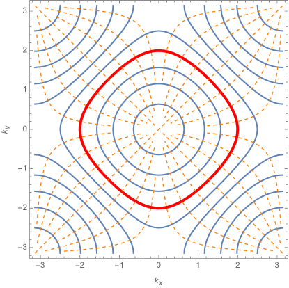
Figure S1: Orthogonal coordinates for a generic FS, denoted by red thick lines.

In this situation, polar coordinates for ${\bm{k}}$ space are no longer useful. Instead one needs to use a proper curvilinear coordinate system for each dispersion relation $\epsilon({\bm{k}})$, which we sketch in Fig. S1. A natrual choice for the radial coordinate is proportional to $\epsilon({\bm{k}})$ itself, which is a constant on the FS. The second coordinate $\tilde{\theta}\in[-\pi,\pi\}$ acts as an angular variable on each contour. For simplicity of the Moyal bracket $\star=\exp[-{i}B{\overleftarrow{\partial_{\bm{k}}}\times\overrightarrow{\partial_{{\bm{k}}}}}/2(1+B\Omega)]$, we choose the second coordinate to be orthogonal to $\epsilon({\bm{k}})$. The phase-space integration measure of $(\epsilon,\tilde{\theta})$ can be seen from the well-known relation

$$\int\frac{dk_{x}dk_{y}}{4\pi^{2}}...=\int{d\epsilon d\tilde{\theta}}\,g(\epsilon,\tilde{\theta})...$$ (S23)

where

$$\int d\tilde{\theta}g(\epsilon,\tilde{\theta})=g(\epsilon),$$ (S24)

is the density of states determined from the dispersion $\epsilon({\bm{k}})$ (not including corrections from Berry phases. [45])

One particular useful choice of $\tilde{\theta}$ is such that the distinct modes in the mode expansion

$$\phi_{i}(\tilde{\theta})=q_{i}+p_{i}\tilde{\theta}+\sum_{n\neq 0}\frac{a_{i,n}}{\sqrt{|n|}}e^{{i}n\tilde{\theta}},~\tilde{\theta}\in[-\pi,\pi),$$ (S25)

are orthogonal, e.g.,

$$\int_{-\pi}^{\pi}d\tilde{\theta}g(\epsilon_{F},\tilde{\theta})e^{{i}(n-m)\tilde{\theta}}\sim\delta_{nm}.$$ (S26)

Obviously, such a choice requires $g(\epsilon_{F},\tilde{\theta})$ to be a constant, i.e., $g(\epsilon_{F},\tilde{\theta})={g(\epsilon_{F})}/{2\pi}$. This can be done as long as the FS is away from van Hove points. We denote the angular variable $\tilde{\theta}$ of this specific coordinate system $\theta$. We emphasize that this is not to be confused with the polar angle from $\Gamma$ point of the BZ.

In the $(\epsilon,\theta)$ coordinates, the phase-space integration measure and the Moyal star product is given by

$$\int\frac{dk_{x}dk_{y}}{2\pi B}(1+B\Omega)...=\int\frac{d\epsilon d\theta}{B}\,g(\epsilon)(1+B\Omega)...,$$ (S27)

$$F\star G=F\exp[-\frac{{i}B}{4\pi}\frac{\overleftarrow{\partial_{\epsilon}}\times\overrightarrow{\partial_{\theta}}}{g(\epsilon)(1+B\Omega)}]G.$$ (S28)

In this coordinate system, Eq. (8) of the main text evaluates to $S_{\rm w}+S_{\rm cb}$, where

$$S_{\rm cb}[\phi]=\frac{1}{2}\int\frac{d\theta dt}{2\pi}\partial_{\theta}\phi\left[\dot{\phi}-\frac{B}{2\pi g(\epsilon_{F})(1+B\Omega(\theta))}\partial_{\theta}\phi\right]$$ (S29)

Focusing on the $(q,p)$ modes of (S25), integrating over $\theta$, and incorporating contributions from $S_{\rm w}$, we obtain

$$S_{\rm zero}[p,q]=\int dt\left[\left(-\frac{\mathcal{A}_{\rm FS}}{2\pi B}-\frac{\gamma}{2\pi}\right)\dot{q}+p\dot{q}-\frac{\bar{\omega}_{c}}{2}p^{2}\right],$$ (S30)

where

$$\bar{\omega}_{c}=\frac{B}{2\pi g(\epsilon_{F})}\left\langle\frac{1}{1+B\Omega(\theta)}\right\rangle_{\rm FS},$$ (S31)

which is Eq. (11) in the main text. There $g(\epsilon_{F})$ is denoted as $g(\epsilon_{F},B)$ to emphasize its dependence on $B$ due to orbital magnetic moments.

III Derivation of the modified Lifshitz-Kosevich formula

In this section, we detail the derivation of the modified Lifshitz-Kosevich formula from bosonization. We start with the part of the free energy from the zero modes

$$F_{\rm zero}=-N_{\phi}T\log\left[\sum_{p=-\infty}^{\infty}{e}^{-{\beta\bar{\omega}_{c}}(p+\Delta/2\pi)^{2}/2}\right]$$ (S32)

where $\Delta=\mathcal{A}_{\rm FS}/B+\gamma$. Using the Poisson resummation formula, it can be rewritten as

$$F_{\rm zero}= -N_{\phi}T\log\left[\int dx\,{e}^{-{\beta\bar{\omega}_{c}}(x+\Delta/2\pi)^{2}/2}+2\sum_{n=1}^{\infty}\int dx\,{e}^{-{\beta\bar{\omega}_{c}}(x+\Delta/2\pi)^{2}/2}\cos(2\pi nx)\right]$$

$$= -\frac{N_{\phi}T}{2}\log\frac{2\pi T}{\bar{\omega}_{c}}-N_{\phi}T\log\left[1+2\sum_{n=1}^{\infty}\cos\left(n\Delta\right){e}^{-{2n^{2}\pi^{2}T}/{\bar{\omega}_{c}}}\right]$$ (S33)

Only the second term contains oscillation in $\Delta$, which is denoted as $F_{\rm osc}$ in the main text.

Note that from the definition of the Jacobi elliptic $\theta$-function [50]

$$\theta_{3}(z,q)=1+2\sum_{n=1}q^{n^{2}}\cos(2nz),~~~|q|<1,$$ (S34)

we can rewrite $F_{\rm osc}$ as

$$F_{\rm osc}=-N_{\phi}T\log\left[\theta_{3}\left(\frac{\Delta}{2},q\right)\right],$$ (S35)

where

$$\Delta=\frac{\mathcal{A}_{\rm FS}}{B}+\gamma,~~q=\exp(-\frac{2n^{2}\pi^{2}T}{\bar{\omega}_{c}}).$$ (S36)

It is well-known that the Jacobi function $\theta_{3}$ has a product representation [50]:

$$\theta_{3}(z,q)=\prod_{n=1}(1-q^{2n})\prod_{n=1}^{\infty}\left[1+2q^{2n-1}\cos(2z)+q^{4n-2}\right].$$ (S37)

Using this, discarding nonoscillatory terms, we get

$$F_{\rm osc}= -N_{\phi}T\sum_{n=1}^{\infty}\log\left[1+2q^{2n-1}\cos(\Delta)+q^{4n-2}\right]$$

$$= -2N_{\phi}T\real\sum_{n=1}^{\infty}\log\left[1+q^{2n-1}{e}^{{i}\Delta}\right].$$ (S38)

Expanding the log and summing over $n$, we obtain

$$F_{\rm osc}= 2N_{\phi}T\real\sum_{n=1}^{\infty}\sum_{k}^{\infty}\frac{(-)^{k}}{k}{q^{(2n-1)k}{e}^{{i}k\Delta}}$$

$$= 2N_{\phi}T\sum_{k}^{\infty}\frac{(-)^{k}}{k}\frac{q^{k}}{1-q^{2k}}\cos\left(k\Delta\right).$$ (S39)

Using (S36), we get

$$F_{\rm osc} =N_{\phi}T\sum_{k=1}^{\infty}A_{k}\cos\left[k\left(\frac{\mathcal{A}_{\rm FS}}{B}+\gamma\right)\right],~~~\textrm{where }A_{k}=\frac{(-)^{k}}{k\sinh\left(2\pi^{2}kT/\bar{\omega}_{c}\right)}.$$ (S40)

This is the modified Lifshitz-Kosevich formula, Eq. (15) in the main text.

IV Relation between $\gamma$ and anomalous Hall conductance

In this section we provide a more detailed derivation relating the Berry phase $\gamma$ around the FS to the anomalous Hall conductance $\sigma_{xy}^{H}$. As we discussed in the main text, the key ingredient of the proof is a UV/IR matching of the braiding algebra. We consider the “translation” operator (setting the lattice constant $a=1$)

$$\hat{\mathbb{T}}_{x,y}=\exp({i}\sum_{{\bm{\pi}}}\hat{N}_{{\bm{\pi}}}\pi_{x,y}),$$ (S41)

and evaluate the braiding algebra $\hat{\mathbb{T}}_{x}\hat{\mathbb{T}}_{y}\hat{\mathbb{T}}_{x}^{-1}\hat{\mathbb{T}}_{y}^{-1}$.

In the UV (lattice scale), we have

$$\hat{\mathbb{T}}_{x,y}=\exp({i}\sum_{i=1}^{N}\widehat{\pi}_{i;x,y}),$$ (S42)

where $N$ is the total particle number and $\widehat{\pi}_{i}$ is the first-quantized kinetic momentum operator for the $i$-th particle. Using the fact that $[\widehat{\pi}_{x},\widehat{\pi}_{y}]=-{i}B$, and the fact that $BL^{2}=2\pi$ (since $N_{\phi}=1$), we obtain

$$\hat{\mathbb{T}}_{x}\hat{\mathbb{T}}_{y}\hat{\mathbb{T}}_{x}^{-1}\hat{\mathbb{T}}_{y}^{-1}=\prod_{i}^{N}\exp(\frac{2\pi{i}}{L^{2}})={e}^{2\pi{i}\nu},$$ (S43)

where $\nu=N/L^{2}$.

In the IR (low energy limit), the translation operator is represented by operators that act near the FS. We have

$$\hat{\mathbb{T}}_{x,y}\sim\exp{{i}\int_{\theta}\hat{n}(\theta)\left[k_{F;x,y}(\theta)\pm B\mathcal{A}_{y,x}(\theta)\right]},$$ (S44)

where $k_{F;x,y}$ are the components of the Fermi momentum and we have used

$$k_{x,y}\equiv\pi_{x,y}\mp B\mathcal{A}_{y,x}.$$ (S45)

Via the Baker-Campbell-Hausdorff formula ${e}^{A}{e}^{B}{e}^{-A}{e}^{-B}=e^{[A,B]}\cdots$, we then have

$$\hat{\mathbb{T}}_{x}\hat{\mathbb{T}}_{y}\hat{\mathbb{T}}_{x}^{-1}=\hat{\mathbb{T}}_{y}\exp{-\int_{\theta,\theta^{\prime}}[\hat{n}(\theta),\hat{n}(\theta^{\prime})]\left(k_{F;x}(\theta)+B\mathcal{A}_{y}(\theta)\right)\left(k_{F;y}(\theta^{\prime})-B\mathcal{A}_{x}(\theta^{\prime})\right)}$$ (S46)

Applying the Kac-Moody algebra

$$[\hat{n}(\theta),\hat{n}(\theta^{\prime})]=\frac{-{i}}{2\pi}\delta^{\prime}(\theta-\theta^{\prime}),$$ (S47)

and integrating by parts we get

$$\hat{\mathbb{T}}_{x}\hat{\mathbb{T}}_{y}\hat{\mathbb{T}}_{x}^{-1}\hat{\mathbb{T}}_{y}^{-1}= \exp[\frac{{i}}{2\pi}\oint\left(k_{F;x}(\theta)+B\mathcal{A}_{y}(\theta)\right){d}\left(k_{F;y}(\theta)-B\mathcal{A}_{x}(\theta)\right)]$$

$$= \exp[\frac{{i}}{2\pi}\oint k_{F;x}(\theta){d}k_{F;y}(\theta)]\exp[\frac{{i}B}{2\pi}\oint\bm{\mathcal{A}}(\theta)\cdot{d}{\bm{k}}_{F}(\theta)],$$ (S48)

where we have kept only $\mathcal{O}(B)$ terms in the exponent, and integrated by parts again in the second factor of the last line. Preforming the integrals, we get

$$\hat{\mathbb{T}}_{x}\hat{\mathbb{T}}_{y}\hat{\mathbb{T}}_{x}^{-1}\hat{\mathbb{T}}_{y}^{-1}=\exp[{i}\frac{\mathcal{A}_{\rm FS}}{2\pi}+{i}\frac{B\gamma}{2\pi}],$$ (S49)

which is Eq. (16) of the main text. Matching UV with IR, i.e., (S43) with (S49), using the Luttinger theorem and the Streda formula, we arrive at Eq. (17) of the main text:

$$\sigma_{xy}^{H}(q\to 0,\omega=0)=\frac{\gamma}{4\pi^{2}}.$$ (S50)