The Sound of Dark Sectors in Pulsar Timing Arrays

Abstract

A phase transition in the dark sector (DS) presents a promising explanation for the stochastic gravitational wave (GW) signals detected in recent observations by Pulsar Timing Arrays (PTAs). Instead of focusing solely on fitting data with phenomenological parameters, we systematically delineate simple, underlying dark sector (DS) models at the microscopic, Lagrangian level and uncover the conditions required to yield the GW spectrum observed by PTAs. We also illustrate the possibilities of the DS cosmology, which may include a dark matter candidate with a $\displaystyle\mathcal{O}$(MeV) mass.

Introduction. Recent measurements from several Pulsar Timing Arrays (PTAs), including NANOGrav, EPTA, PPTA, and CPTA [1, 2, 3, 4, 5, 6, 7, 8], have provided strong evidence for quadrupolar Hellings-Downs correlations [9], potentially indicating the discovery of a stochastic gravitational wave background (SGWB) in the nanohertz frequency range. These findings signal a new chapter in gravitational wave (GW) cosmology and prompt the critical question of the origin of this observation. A potential origin of the signal is GW emission from a large population of coalescing supermassive black holes [10, 11, 12, 13, 14, 15, 16, 17, 18]. However, the specifics of the astrophysical mechanisms capable of generating the observed signal remain an active area of investigation [19, 20]. Alternatively, beyond the Standard Model (SM) physics offers compelling cosmological sources of the signal [21, 22, 23, 24, 25, 26, 27, 28, 29, 30], and precise measurements of the signal may open up exciting opportunities to probe the microscopic details of the underlying new physics in the near future. In this work, we focus on the generally appealing possibility that the PTA signal originates from SGWB generated during a phase transition (PT) in a dark sector (DS), and explore the connections between the specifics of the GW spectrum and the characteristics of the DS.

GWs originating from PTs [31] have been widely studied in the context of the electroweak PT, whereby beyond the Standard Model (SM) physics is required to render it strong first-order for generating detectable GWs (see, e.g., Refs. [32, 33, 34, 35, 36, 37, 38, 39, 40]). In these cases, the predicted GW signal can be within the LISA frequency range [41, 42], offering potential complementarity between related collider searches and future GW observations. Recent years have seen increasing interest in PTs occurring solely within a DS [43, 44, 45, 46, 47, 48, 49, 50], with its own scalar potentials and, potentially gauge symmetries, which allows for a strong first-order PT. GW signatures would serve as a promising means for probing such a DS, in particular when its non-gravitational interaction with the SM is absent or feeble.

Most of the existing related studies [22, 51, 52, 23] focused on parameterizing DS PTs with macroscopic quantities, such as the energy density of DS, the temperature and duration of the PT. Only a few studies [51, 53, 54, 55] have investigated microscopic details of the DS that underlie the observed PTA spectra. To address this gap, we delineate minimal DS models with perturbative dynamics that can realize a strong first-order PT, involving gauge and fermionic fields, as inspired by the electroweak sector of the SM. We perform a systematic general study of the first-order PT in such models and the resultant GW signatures, with a focus on fitting the PTA observations. We also identify potential dark matter (DM) candidates from the DS and its plausible cosmological history.

The rest of this Letter is organized as follows. We first introduce the minimal DS models of interest and demonstrate the conditions for realizing a strong first-order PT. Then, we estimate the SGWB from the benchmark models and analyze how well they fit the PTA data. Following that, we discuss the implications for the DS cosmology based on the properties of the DS model as required by fitting PTA observations. Finally, we conclude.

Dark Sector Phase Transitions. We start by systematically laying out the minimal model setup that enables us to perform a perturbative analysis and demonstrate the key characteristics of models that generate GWs consistent with the PTA observations. A PT typically originates from the spontaneous breaking of a symmetry, which immediately requires a scalar degree(s) of freedom. To realize a strong first-order PT enabling detectable GW signals, additional bosonic degrees of freedom interacting with this scalar are typically required. We therefore consider a DS with a gauged dark U$\displaystyle(1)$ symmetry, spontaneously broken when a complex scalar $\displaystyle\Phi$ acquires a vacuum expectation value (VEV). To allow for a Yukawa coupling $\displaystyle y_{D}$, we introduce a dark U$\displaystyle(1)$ charged fermion $\displaystyle(\Psi)$ and a dark U$\displaystyle(1)$ singlet fermion $\displaystyle(\chi)$. All these fields are singlets under the SM gauge group. The Lagrangian relevant to the PT is then of the form

$$\mathcal{L}_{\rm{DSPT}}\supset(D^{\mu}\Phi)^{{\dagger}}(D_{\mu}\Phi)+\mu^{2}\,\Phi^{{\dagger}}\Phi-\frac{\lambda}{2}(\Phi^{{\dagger}}\Phi)^{2}-y_{D}\,\bar{\Psi}\Phi\chi\,,$$ (1)

where the covariant derivative $\displaystyle D_{\mu}\Phi=\partial_{\mu}\Phi+ig_{D}A^{\prime}_{\mu}\Phi$ couples the scalar to the dark gauge boson $\displaystyle A^{\prime}_{\mu}$ with coupling strength $\displaystyle g_{D}$. We take $\displaystyle\mu^{2}>0$ and $\displaystyle\lambda>0$ to ensure the stability of the potential and allow $\displaystyle\Phi$ to acquire a nonzero VEV $\displaystyle v_{0}$,

$$\langle\Phi\rangle=\frac{v_{0}+\phi}{\sqrt{2}}\,.$$ (2)

Here, $\displaystyle\phi$ is the physical, dark Higgs, and $\displaystyle v_{0}=\sqrt{\mu^{2}/\lambda}$ is the VEV at $\displaystyle T=0$, and we adopt unitary gauge to gauge away the Goldstone boson. For generality, we also consider larger gauge groups such as SU$\displaystyle(N)$, by promoting $\displaystyle\Phi$ and $\displaystyle\Psi$ to multiplets in representations of SU$\displaystyle(N)$. However, in order to eliminate relic massless degrees of freedom after the PT, which can be subject to strong constraints from Big Bang Nucleosynthesis (BBN) and the Cosmic Microwave Background (CMB) observations, in particular in the form of the effective number of new relativistic neutrino degrees of freedom $\displaystyle\Delta N_{\rm{eff}}$ [56, 57, 58, 59], we assume maximal breaking of SU$\displaystyle(N)$. As an example, for SU$\displaystyle(2)$, we take $\displaystyle\Phi$ in the fundamental representation and choose the following configuration at the minimum of the scalar potential

$$\langle\Phi\rangle=\left[0,\,\frac{v_{0}+\phi}{\sqrt{2}}\right]^{T}\,,$$ (3)

which maximally breaks SU$\displaystyle(2)$, resulting in 3 massive gauge bosons. For larger $\displaystyle N$, the VEV configuration needs to be specifically tailored . We thus assume that the $\displaystyle N^{2}-1$ gauge bosons acquire equal masses from the PT when evaluating the effective potential (see App. A). Our discussion is largely insensitive to the specifics of VEV choices.

Based on the DS model presented, we can then calculate the phenomenological parameters that characterize the PT: $\displaystyle T_{*}$, the temperature at which the PT occurs; $\displaystyle\beta/H_{\ast}$, the inverse time duration of the PT; and $\displaystyle\alpha_{\ast}$, the latent heat released in the PT, normalized to the total radiation density of the universe at the time of the PT. All of these quantities are derived from the bubble nucleation rate of the true vacuum and, therefore, ultimately derived from the finite-temperature effective potential (see App. A). The GW spectrum depends on these PT parameters, which in turn depend on the underlying model parameters such as $\displaystyle\lambda$ and $\displaystyle g_{D}$. Therefore, in order to facilitate our discussion in the context of the PTA data, we systematically analyze how the phenomenological PT parameters depend on the parameters in the model’s Lagrangian.

To begin, we consider the U$\displaystyle(1)$ model with $\displaystyle y_{D}=0$, and isolate the effect of the dimensionful parameter $\displaystyle\mu$. The quartic self-coupling has a milder effect on PT, so we assume $\displaystyle\lambda=0.05$ without loss of generality and study the dependence of $\displaystyle T_{*}$ in the ($\displaystyle\mu$, $\displaystyle g_{D}$) plane. Fig. 1 shows that the $\displaystyle\mu$ parameter essentially determines the scale of $\displaystyle T_{*}$, so we set $\displaystyle\mu=2$ MeV for our further analysis. Note that for the fixed value of $\displaystyle\lambda=0.05$, above $\displaystyle g_{D}\sim 1.3$, the bubble nucleation rate never becomes comparable to the Hubble expansion rate (see Eq. A.14 of App. A), implying that the scalar field is trapped in the false minimum. Below $\displaystyle g_{D}\sim 1.1$, the PT is no longer first-order, and the high $\displaystyle T$ minimum smoothly crosses over to the true minimum at $\displaystyle T=0$. These results are nearly identical for SU$\displaystyle(2)$ and SU$\displaystyle(3)$ as, although the precise value of $\displaystyle T_{*}$ depends on the couplings and number of gauge bosons in the effective potential (c.f. App. A), its magnitude is primarily influenced by $\displaystyle\mu$.

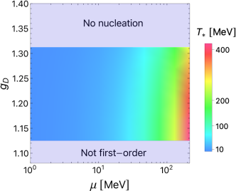
Figure 1: Density plot for $\displaystyle T_{*}$ in the plane of $\displaystyle(\mu,\,g_{D})$ for the U$\displaystyle(1)$ model with $\displaystyle y_{D}=0$ and $\displaystyle\lambda=0.05$. Analogous plots for SU$\displaystyle(2)$ and SU$\displaystyle(3)$ models are nearly identical.

We now study the dependence of the remaining PT parameters, $\displaystyle\beta/H_{*}$ and $\displaystyle\alpha_{*}$, on the bosonic couplings $\displaystyle\lambda$ and $\displaystyle g_{D}$, which we show in Fig. 2 for the example of U$\displaystyle(1)$ model. We see that $\displaystyle\beta/H_{*}$ first decreases and then increases as $\displaystyle g_{D}$ and $\displaystyle\lambda$ increase, with a minimum $\displaystyle\sim 1$. As for the PT strength $\displaystyle\alpha_{*}$, it tends to peak as it gets closer to the boundary where bubble nucleation ceases to occur. This is because the gauge coupling increases with a fixed $\displaystyle\lambda$, a potential barrier forms which requires more energy to tunnel through to the true vacuum; and beyond a certain value of $\displaystyle g_{D}$ the scalar field can no longer tunnel to the true minimum due to the barrier. We further examine the effect of enlarging the symmetry group, finding that the aforementioned trends for $\displaystyle\alpha_{*}$ and $\displaystyle\beta/H_{*}$ observed in the U$\displaystyle(1)$ model persist qualitatively for SU$\displaystyle(2)$ and SU$\displaystyle(3)$. However, the parameter space “tilts”: for the same value of $\displaystyle\lambda$, a smaller $\displaystyle g_{D}$ is required, as indicated by the boundaries in Fig. 2. This is due to the increase in the number of massive gauge bosons that appear at loop level, thereby modifying the effective potential (see App. A).

Finally, we analyze the effects of $\displaystyle y_{D}\neq 0$ on the existing parameter space. In Fig. 3, we see that by introducing $\displaystyle y_{D}$, the allowed values of $\displaystyle g_{D}$ can be extended beyond the previous limits (compared to Fig. 2). This can be understood as follows: the fermionic contribution to the effective potential carries a negative sign, in contrast to the positive contribution of bosons; therefore, a certain target of potential form may be maintained with a larger value of gauge coupling, due to the compensation from the fermionic contribution. Nevertheless, for a fixed $\displaystyle g_{D}$, as $\displaystyle y_{D}$ increases further, the negative contribution from the fermions may result in the PT becoming cross-over and beyond a certain value, the effective potential becomes unbounded.

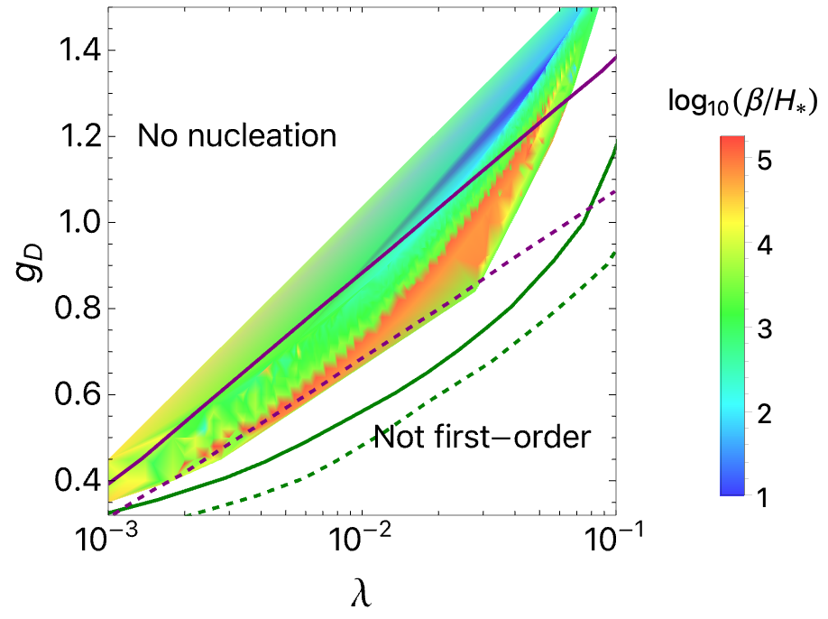
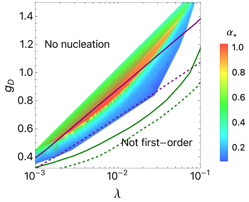
Figure 2: Density plots of PT parameters $\displaystyle\beta/H_{\ast}$ and $\displaystyle\alpha_{\ast}$ in the $\displaystyle(\lambda,\,g_{D})$ plane for the pure gauged sectors (i.e. $\displaystyle y_{D}=0$), with fixed $\displaystyle\mu=2$ MeV. Colored regions correspond to the U$\displaystyle(1)$ model. Similar features are obtained for SU$\displaystyle(2)$ and SU$\displaystyle(3)$ (uncolored). Purple lines show the edges for SU$\displaystyle(2)$ (solid) and SU$\displaystyle(3)$ (dashed) above which the nucleation criterion is not met, and dark green lines give the boundary above which the PT remains first-order for SU$\displaystyle(2)$ (solid) and SU$\displaystyle(3)$ (dashed).

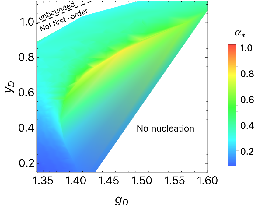
Figure 3: Density plot of $\displaystyle\alpha_{*}$ in the $\displaystyle(g_{D}\,,\,y_{D})$ plane for the U$\displaystyle(1)$ model with fixed $\displaystyle\lambda=0.05$ and $\displaystyle\mu=2$ MeV.

In summary, the PT parameters are mainly affected by bosonic couplings to the scalar driving the PT. The parameter $\displaystyle\mu$ determines the scale of the PT temperature $\displaystyle T_{*}$. We have assumed $\displaystyle\mu=2$ MeV for our discussion, as a PT in the MeV range typically results in a peak frequency of GW in the PTA regime [45, 61, 22] ($\displaystyle f_{\rm peak}\propto T_{*}$, see Eq. B.3 in the Appendix. B). Increasing the quartic and gauge couplings together first increases and then decreases the duration of the PT, with the longest PTs (with $\displaystyle\beta/H_{*}\sim 1$) featuring $\displaystyle\lambda\sim 0.05$ and $\displaystyle g_{D}\sim 1.2$. Increasing $\displaystyle g_{D}$ while keeping $\displaystyle\lambda$ fixed, the PT tends to be stronger because of the additional latent heat released, which peaks at about $\displaystyle\alpha_{*}\sim 1$ and then decreases slightly. We numerically scanned for $\displaystyle\sim 1500$ points in parameter space, within the perturbative ranges of $\displaystyle\lambda\in[10^{-3},\,10^{-1}]$ and $\displaystyle g_{D}\in[0.2,\,2.0]$. As we shall see, pairings of $\displaystyle(\lambda,\,g_{D})$ that result in a large $\displaystyle\alpha_{*}$ and a small $\displaystyle\beta/H_{*}$ are preferred to achieve the sufficient amplitude of GWs as observed by PTAs.

GW Signal for PTAs. A first-order PT proceeds through the nucleation of bubbles of the true phase, from which GWs can be generated from their collisions [62, 63, 64, 65], as well as through sound waves [66, 67, 68] and magneto-hydrodynamic turbulence [69, 70, 71] induced by the interaction of the bubbles with the surrounding plasma,

$$\Omega_{\rm{GW}}h^{2}(f)=\Omega^{\rm{bc}}_{\rm{GW}}h^{2}(f)+\Omega^{\rm{sw}}_{\rm{GW}}h^{2}(f)+\Omega^{\rm{turb}}_{\rm{GW}}h^{2}(f)\,,$$ (4)

where $\displaystyle\Omega_{\rm GW}$ is today’s GW energy density (per logarithmic momentum interval) over the critical energy density. The relative importance of the different contributions depends on the microphysics of the first-order PT. For example, if the scalar field has strong interactions with the surrounding plasma, the sound wave and turbulence contributions tend to be larger, which is our case for a strong first-order PT. We assume that the first-order PT occurs in the “detonation regime”, where the bubble wall velocity exceeds the speed of sound, $\displaystyle v_{w}>1/\sqrt{3}$. In App. B, we review the analytical expressions used to obtain the GW spectra for our analysis.

The GW spectrum depends on the PT parameters in the following manner: $\displaystyle T_{*}$ determines the peak location, while $\displaystyle\alpha_{*}$ and $\displaystyle\beta/H_{*}$ determine the size and shape of the spectrum. These, in turn, depend on the Lagrangian parameters, as discussed in the previous section, translating the dependence of the GW spectrum down to the model parameters: $\displaystyle\{\mu,\,\lambda,\,g_{D},\,y_{D},\,N\}$. We illustrate this through Fig. 4 for the simplest case of the U$\displaystyle(1)$ model, with $\displaystyle y_{D}=0$ and $\displaystyle\lambda=0.05$. Varying $\displaystyle\mu$ affects $\displaystyle T_{*}$ and thus changes the location of the peak frequency. A decrease (increase) in $\displaystyle\beta/H_{*}$ causes the spectrum to shift diagonally to the right (left), while an increase (decrease) in $\displaystyle\alpha_{*}$ directly increases (decreases) the amplitude. Therefore, the gauge coupling $\displaystyle g_{D}$ (for a fixed $\displaystyle\lambda$) essentially determines $\displaystyle\alpha_{*}$ and $\displaystyle\beta/H_{*}$ (see also Fig. 2). Finally, the turbulence effect typically leads to a component in the spectrum with a higher peak frequency (see App. B), modifying the tails of the spectra.

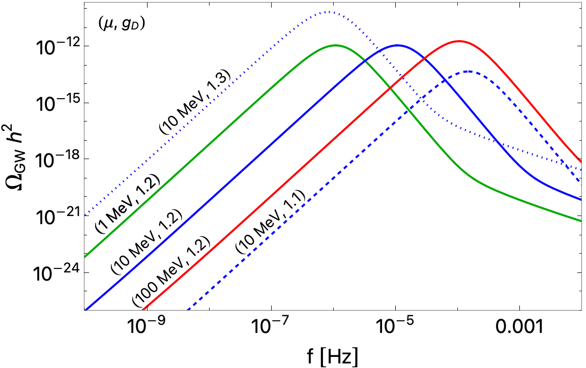
Figure 4: Examples of the GW spectrum for various parameters in the U$\displaystyle(1)$ case. Here, we have fixed $\displaystyle\lambda=0.05$ and $\displaystyle y_{D}=0$ for all curves and $\displaystyle(\mu,g_{D})$ is indicated in parentheses. The solid-colored curves have the same $\displaystyle g_{D}=1.2$, but different $\displaystyle\mu$. The dotted and dashed curves have the same $\displaystyle\mu$, but different $\displaystyle g_{D}$.

We now study the model parameter space that is consistent with the PTA data from NANOGrav [2], EPTA [4, 5] and PPTA [7]. For our analysis, we consider the mean values and $\displaystyle 1\sigma$ error bars extracted from the PTA violin plots, as computed in Ref. [23] . To quantify the compatibility of the model with the PTA data, we employ a goodness-to-fit metric $\displaystyle\chi^{2}$, defined as

$$\chi^{2}=\sum_{i}\left[\frac{\log\Omega_{\text{GW}}h^{2}(f_{i})-\log\Omega^{\rm{data}}_{\text{GW}}h^{2}(f_{i})}{\Delta\log\Omega^{\rm{data}}_{\text{GW}}h^{2}(f_{i})}\right]^{2}\,,$$ (5)

where $\displaystyle\log\equiv\log_{10}$. $\displaystyle\Omega^{\rm{data}}_{\text{GW}}(f)$ refers to the mean value of the PTA data. $\displaystyle f_{i}$ refers to the frequency of the $\displaystyle i^{\rm{th}}$ bin and we sum over the full PTA data set. As the error bars $\displaystyle\Delta\log\Omega^{\rm{data}}_{\text{GW}}(f_{i})$ are asymmetric, we use the upper or lower error value depending on whether the model prediction lies above or below the mean value.

To evaluate the significance level of the fit, we need to identify the number of degrees of freedom (d.o.f.). We do so by first noting that the sample size is given by the full PTA data set of 41 bins. The number of free parameters is determined by the model we are considering. Assuming no prior constraints on these parameters, we arrive at the d.o.f. given by

$$\displaystyle n \displaystyle=41-n_{\rm{params}}\,.$$ (6)

For a systematic study, we approach the model parameter space as follows: we fix the gauge group (i.e. $\displaystyle N$) and then consider the case with and without $\displaystyle y_{D}=0$. This is demonstrated in Fig. 5 for the U$\displaystyle(1)$ case with $\displaystyle y_{D}=0$. First, fixing $\displaystyle\mu=2$ MeV, we make use of the results of Fig. 2 to locate the minimum $\displaystyle\chi^{2}$ value (d.o.f. = 39), corresponding to $\displaystyle(\lambda,\,,g_{D})$ that leads to an optimal combination of $\displaystyle\beta/H_{*}$ and $\displaystyle\alpha_{*}$ to fix the amplitude of the signal. With these couplings determined, we then vary $\displaystyle\mu$ to find the minimum $\displaystyle\chi^{2}$ (d.o.f. = 40), which determines the $\displaystyle T_{*}$ and therefore anchors the peak frequency. For our likelihood analysis, we note that a fit at the significance level of $\displaystyle 1\sigma$ corresponds to $\displaystyle\chi^{2}\sim 45$, while $\displaystyle\chi^{2}\sim 60\,(70)$ corresponds to a fit at the level of $\displaystyle 2\sigma\,(3\sigma)$. We adopt a similar approach when analyzing the fitting in the cases of SU$\displaystyle(2)$ and SU$\displaystyle(3)$ models.

According to Fig. 5, once the phenomenological parameters $\displaystyle\alpha_{*}$ and $\displaystyle\beta_{*}/H$ are pinned down by the PTA data, the underlying model parameters are precisely defined. This is a common feature for all the models we considered in this work. In Tab. 1, we show the parameters that provide the best fit for the PTA signal, and Fig. 6 shows the corresponding GW spectra.

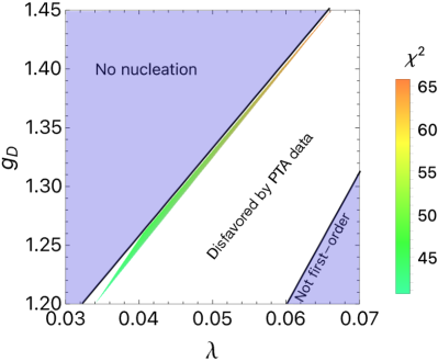
Figure 5: Fitting results for the U$\displaystyle(1)$ model with $\displaystyle y_{D}=0$. Top: $\displaystyle\chi^{2}$ values for up to a $\displaystyle 3\sigma$ fit to PTA data in the $\displaystyle(\lambda,g_{D})$ plane, with fixed $\displaystyle\mu=2$ MeV, to identify the optimal coupling. The white region is disfavored by the PTA fit. Bottom: $\displaystyle\chi^{2}$ as a function of $\displaystyle\mu$ for fixed $\displaystyle(\lambda,g_{D})=(0.034,\,1.2)$ from the top plot.

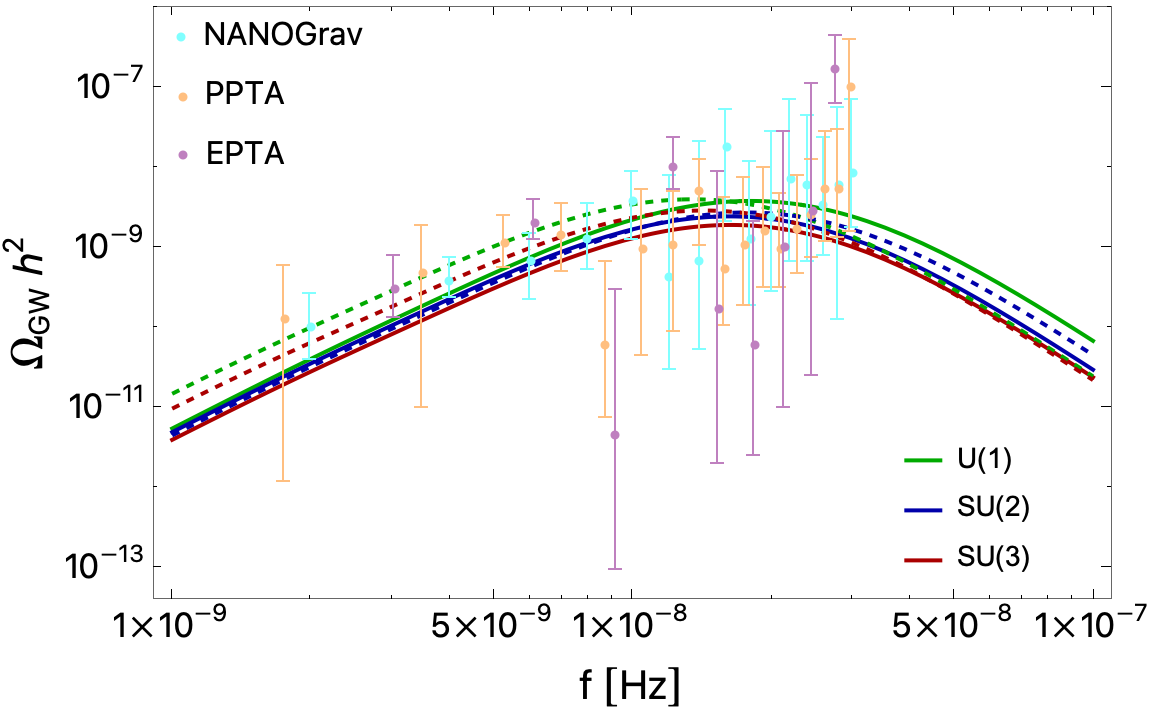
Figure 6: The best-fit GW spectra from DS PTs we consider in this work, with the NANOGrav, PPTA and EPTA datasets considered in our analysis superimposed. Colored lines indicate the gauge group, whereas dashed lines indicate the corresponding gauge sector includes fermions (i.e. $\displaystyle y_{D}\neq 0$).

MODEL	$\displaystyle(\mu,\,\lambda,\,g_{D},\,y_{D})$	$\displaystyle(T_{*},\,\alpha_{*},\,\beta/H_{*})$	$\displaystyle\chi^{2}$
U$\displaystyle(1)$	(2.4 MeV, 0.03, 1.2, 0)	(2.4 MeV, 0.96, 47)	36
	(2.7 MeV, 0.06, 1.5, 0.8)	(2.5 MeV, 0.76, 38)	29
SU$\displaystyle(2)$	(2.0 MeV, 0.05, 1.1, 0)	(1.9 MeV, 0.79, 58)	30
	(2.2 MeV, 0.05, 1.2, 0.7)	(2.0 MeV, 0.83, 54)	38
SU$\displaystyle(3)$	(1.8 MeV, 0.03, 0.7, 0)	(1.8 MeV, 1.06, 70)	40
	(2.3 MeV, 0.05, 0.9, 0.6)	(2.1 MeV, 0.85, 43)	31

Table 1: The best-fit model parameters corresponding to the GW spectra in Fig. 6, with the calculated PT parameters in the third column. The d.o.f. is on average 40 implying all these points correspond to a fit at $\displaystyle 1\sigma$ confidence level (see text for details).

Implications for the Dark Sector Cosmology. With the theoretical prior that the recently observed PTA signal originates from the DS models we consider, the PTA measurements provide precise conditions on the DS parameters for a given model, allowing us to examine in detail the thermal history of the DS and the potential dark matter (DM) candidate therein. We will focus on the U$\displaystyle(1)$ model as an example for illustration. Given that this letter primarily addresses the DS PT and GW production, we will only outline the main features of the DS cosmology after the PT and examine the viable outcomes of the residual energy density contained in the DS. The DS thermal history depends on additional model specifics (beyond what is required to explain the GW signal), and we defer a detailed investigation of the DS cosmology to future studies.

We first identify the typical DM candidate in our benchmark models by considering the mass spectrum of the new particles involved. The dark Higgs $\displaystyle\phi$ has a physical mass of $\displaystyle\sqrt{2\mu^{2}}\sim 3$ MeV. In the U$\displaystyle(1)$ model, the gauge boson $\displaystyle A^{{}^{\prime}}_{\mu}$ acquires a mass of $\displaystyle\sim 8$–$\displaystyle 15~\mathrm{MeV}$, while acquired fermion masses range from $\displaystyle\sim 5$–$\displaystyle 10~\mathrm{MeV}$ when Yukawa couplings are included. Therefore, in the absence of non-gravitational interactions with the SM, $\displaystyle\phi$ is the lightest stable particle in the DS, potentially a DM candidate.

The $\displaystyle\mathcal{O}(1-10)$ MeV scale masses and the large couplings $\displaystyle(\lambda,g_{D},y_{D})$ ensure that the $\displaystyle 2-2$ scattering and annihilation rates between DS particles well exceed the Hubble expansion rate $\displaystyle H(T\sim{\rm MeV})\sim T^{2}/M_{\rm pl}\sim 10^{-22}$ MeV at the PT time $\displaystyle T\sim$ MeV ($\displaystyle M_{\rm pl}=1.22\cdot 10^{19}$ GeV is the Planck mass). Even the number-changing process $\displaystyle 3\phi\to 2\phi$, facilitated by the $\displaystyle\lambda\phi^{4}$ and $\displaystyle\lambda v_{0}\phi^{3}$ couplings after the U$\displaystyle(1)$ breaking, has a rate $\displaystyle n_{\phi}^{2}\sigma_{3\phi\to 2\phi}\sim 10^{-12}(\lambda/10^{-2})^{4}~$MeV around $\displaystyle T\sim$ MeV, thus is highly efficient. This ensures that the DS particles remain in both kinetic and chemical equilibrium, and most of the DS energy density after the PT is stored in the lightest particle $\displaystyle\phi$.

As we have seen, to produce sufficient GW as observed by PTAs, the energy in the DS during PT (mainly in the form of latent heat) is comparable to that of the SM (as indicated by $\displaystyle\alpha_{*}\sim 1$ in our best-fit results). After the PT, latent heat is generally released through the production of dark-sector particles. If such a large DS energy remains in the DS until later times, the model is subject to strong constraints from BBN [73, 61] and CMB [59] observations (by modifying the Hubble expansion rate), which allow the DS energy density to be at most $\displaystyle\sim 10\%$ of the SM photon energy (often expressed in terms of $\displaystyle\Delta N_{\rm eff}$). Therefore, the DS cannot be fully decoupled from the SM, and its energy must be efficiently released to the SM through certain portal interactions, after the PT and before the BBN era. With the preferred $\displaystyle\alpha_{*}\sim 1$ for fitting the PTA signal, BBN observation poses a constraint of $\displaystyle T_{*}\gtrsim 2$ MeV [61]. Some of the best-fit parameters in Table 1 can, therefore, lead to potential tensions with this BBN constraint. However, this tension may be alleviated by slightly compromising the significance level of the fit: e.g. for the SU$\displaystyle(3)$ case with $\displaystyle y_{D}=0$ in Tab. 1, if $\displaystyle\mu$ increases from $\displaystyle 1.8$ MeV to 2.4 MeV, consequently giving $\displaystyle T_{*}\sim 2.3$ MeV, then the fitting would be at the level of about $\displaystyle 2\sigma$.

Given the closeness in time between $\displaystyle T_{*}$ and BBN time, as revealed from our fitting results, this requirement leads to special conditions on the DS cosmology. The possibilities may be categorized in terms of the cosmological role of $\displaystyle\phi$: first, the portal interaction enables the decay of $\displaystyle\phi$ before BBN; second, $\displaystyle\phi$ is stable or long-lived enough to be (all or a fraction of) DM while releasing excess energy through certain annihilation/freeze-out processes.

Notably, even in the case that $\displaystyle\phi$ is DM, a portal coupling to the SM is still required for viability. Assuming there is no coupling to the SM, the dominant annihilation channel for $\displaystyle\phi$ to remain in thermal equilibrium is the number-changing process $\displaystyle 3\phi\to 2\phi$ [74, 75, 76]. For $\displaystyle m_{\phi}\approx 3$ MeV and including the Boltzmann suppression $\displaystyle\exp(-m_{\phi}/T)$ in $\displaystyle n_{\phi}$, one can estimate that the freeze-out of $\displaystyle\phi$ happens around $\displaystyle T_{\rm dec}\sim 0.35$ MeV, and the relic abundance of $\displaystyle\phi$ today is $\displaystyle\Omega_{\phi}h^{2}\sim 10^{2}$, which poses an overclosure problem [59].

The above discussions clarify that effective portal couplings between the DS and the SM are required to satisfy the related cosmological constraints. However, this is not trivial to realize, given the associated laboratory bounds on the portal couplings. In the following, we discuss a few simple options.

First, the simplest option one may consider is to invoke a mixing between $\displaystyle\phi$ and the SM Higgs via the $\displaystyle|H|^{2}|\phi|^{2}$ coupling, so that $\displaystyle\phi$ decays before BBN. However, at $\displaystyle m_{\phi}=3$ MeV, constraints from collider searches require $\displaystyle\theta\>\raisebox{-2.15277pt}{$\displaystyle\stackrel{{\scriptstyle\textstyle<}}{{\sim}}$}\>10^{-5}$ [77, 78], resulting in a long lifetime of $\displaystyle\phi$ that violates the BBN bound [79].

Now, we consider other possibilities for the portal interaction where $\displaystyle\phi$ may be DM, such as the kinetic mixing between the $\displaystyle U(1)$ $\displaystyle A_{\mu}^{\prime}$ and the SM photon through $\displaystyle\epsilon F^{\prime}_{\mu\nu}F^{\mu\nu}$. In the absence of dark fermions, or if the dark fermion masses are larger than $\displaystyle m_{A^{\prime}}/2$, $\displaystyle A_{\mu}^{\prime}$ predominantly decays into SM $\displaystyle e^{+}e^{-}$. The decay can occur before BBN for $\displaystyle m_{A^{\prime}}\lesssim 10\,\mathrm{MeV}$ with $\displaystyle\epsilon\approx 10^{-9}$ that satisfies the bounds from supernova cooling [80, 81]. In this case, the depletion of $\displaystyle\phi$ energy would therefore proceed through the forbidden DM channel annihilation [83, 84], where $\displaystyle\phi\phi\to A^{\prime}A^{\prime}$ (via the $\displaystyle\phi^{2}A_{\mu}^{\prime}A^{{}^{\prime}\mu}$ coupling) annihilates the lighter $\displaystyle\phi$ into the heavier $\displaystyle A^{\prime}$ (as in our benchmarks typically $\displaystyle m_{A^{\prime}}>m_{\phi}$), followed by the subsequent $\displaystyle A^{\prime}\to e^{+}e^{-}$ decay. The freeze-out temperature $\displaystyle T_{F}$ and, consequently, the relic density of $\displaystyle\phi$ are sensitive to the model parameters such as mass splitting $\displaystyle(m_{A^{\prime}}-m_{\phi})$, with the potential to accommodate $\displaystyle\phi$ as a viable candidate for DM, e.g. with $\displaystyle m_{\phi}=3$ MeV, $\displaystyle(m_{A^{\prime}}-m_{\phi})/m_{\phi}\approx 1$ and $\displaystyle m_{\phi}/T_{F}\approx 15$. Recent studies show that models with a light scalar DM that efficiently scatter with a dark photon through $\displaystyle\epsilon F^{\prime}_{\mu\nu}F^{\mu\nu}$ may be subject to additional BBN constraints due to energy injection into SM electrons and photons, placing a constraint on the scalar mass $\displaystyle m\gtrsim 3$ MeV  [85, 86, 87].

Alternatively, a viable scenario of $\displaystyle\phi$ as DM can be realized by the ELDER mechanism [88, 89], where the DM relic abundance is determined by a combination of efficient elastic scattering with SM and self-annihilation such as $\displaystyle 3\phi\to 2\phi$. For our consideration, a sufficient portal coupling can be realized by kinetic mixing $\displaystyle\epsilon^{\prime}$ (with a much weaker constraint than the simple kinetic mixing as we discussed above) between the DS U$\displaystyle(1)$ and an anomaly-free lepton number gauge symmetry U$\displaystyle(1)_{L_{\mu}-L_{\tau}}$ (with gauge coupling $\displaystyle g_{\mu-\tau}$) [90, 91]. In particular, with $\displaystyle\epsilon^{\prime}\approx 10^{-3}$ and $\displaystyle g_{\mu-\tau}\approx 10^{-4}$ (which satisfies the current bound [92, 93, 94, 95]), the equilibrium between DS and SM can be maintained by the dark fermion scattering off SM neutrinos $\displaystyle\psi\,\nu\to\psi\,\nu$ (through the exchange of $\displaystyle A^{\prime}$) and the kinetic equilibrium between $\displaystyle\phi$ and $\displaystyle\psi$, until a freezeout temperature $\displaystyle T_{F}\sim 0.1$ MeV, thereby resulting in $\displaystyle\phi$ with the observed DM relic density . Note that this process heats SM neutrinos by $\displaystyle\mathcal{O}(10\%)$, which requires a dedicated study to assess their impact on BBN and CMB.

Conclusion. In this work, we systematically investigate the possibility of addressing the recent PTA observations with SGWB sourced by phase transitions in dark sectors. We identify minimal DS models with perturbative dynamics that can explain the signal: involving a U$\displaystyle(1)$ or SU$\displaystyle(N)$ gauge symmetry, a Higgs-like scalar, with or without Yukawa coupling to dark fermions. With the details of the underlying model identified, the PTA data reveal specific conditions of the DS properties. In particular, using a likelihood analysis to fit the predicted GW signal to the NANOGrav+EPTA+PPTA data sets, we find that the PT energy scale is pinned down at the $\displaystyle\mathcal{O}$(MeV) scale. For example, in the U$\displaystyle(1)$ model, the SM singlet dark Higgs mass lies in a $\displaystyle 2\sigma$ window of $\displaystyle m_{\phi}\approx 3\pm 0.6$ MeV, the U$\displaystyle(1)$ gauge coupling $\displaystyle g_{D}\approx 1.25\pm 0.05$, and the dark Higgs self-coupling $\displaystyle\lambda\approx 0.04\pm 0.01$. The dark Higgs is potentially a candidate for DM. This information allows us to further elucidate the thermal history of the DS following the PT. In order to produce sufficient GW signal to address the PTA data, the DS energy density around the PT must be comparable to that of the SM sector. In order to be compatible with BBN constraints in such scenarios, a portal coupling to the SM is necessary to transfer the entropy from the DS to the SM. We considered a few examples of such portal couplings and the connection with known scenarios such as forbidden DM, SIMP, and ELDER. A dedicated study of DS cosmology and the potential complementarity with other astrophysical or laboratory searches is beyond the scope of this work, yet worth future pursuit. Finally, although the study was inspired by the recent PTA observations, it is desirable to extend it by examining the DS across various energy scales, which could produce detectable GWs across a broad frequency range, a direction we plan to pursue in future work.

Acknowledgments. We thank Anish Ghoshal and Felix Kahlhoefer for useful discussions. AB is supported by the Basic Science Research Program through the National Research Foundation of Korea (NRF) funded by the Ministry of Education under grant numbers [NRF-2021R1C1C1005076, 2020R1I1A3068803]. YC is supported by the US Department of Energy under award number DE-SC0008541. YDT thanks the generous support from the LANL Director’s Fellowship. This research is partially supported by LANL’s Laboratory Directed Research and Development (LDRD) program. This research was partly supported by grant NSF PHY-2309135 to the Kavli Institute for Theoretical Physics (KITP). YT is supported by grant NSF PHY-2412701. YT would like to thank the Tom and Carolyn Marquez Chair Fund for its generous support. This work was partially performed at the Aspen Center for Physics, supported by National Science Foundation grant No. PHY-2210452.

Appendix A Thermodynamics of a first-order PT

In this appendix, we briefly review the key quantities to describe a first-order PT and determine the associated PT parameters required for the GW spectrum, from a model Lagrangian such as in Eq. 1.

We begin with the effective potential at finite temperature, which we compute at one-loop in this work. As is customary, one first promotes the VEV $\displaystyle v_{0}$ in (2) to a background field $\displaystyle\varphi$. One then obtains the following scalar potential in terms of this background field

$$V_{0}(\varphi)=-\frac{1}{2}\mu^{2}\varphi^{2}+\frac{1}{4}\lambda\varphi^{4}\,,$$ (A.1)

with the tree-level VEV occurring at the minimum of this potential, $\displaystyle v^{2}_{0}=\mu^{2}/\lambda$. The field-dependent masses for the dark Higgs, Goldstone bosons, gauge bosons, and fermions are

$$\displaystyle m^{2}_{\phi}(\varphi)=3\lambda\varphi^{2}-\mu^{2}\,,\quad m^{2}_{\eta}(\varphi)=\lambda\varphi^{2}-\mu^{2}\,,$$ (A.2)

$$\displaystyle m^{2}_{A^{\prime}}(\varphi)=\frac{1}{2}g^{2}_{D}\varphi^{2}\,,\quad m^{2}_{\psi}(\varphi)=\frac{1}{2}y^{2}_{D}\varphi^{2}\,.$$ (A.3)

The finite-temperature effective potential at one-loop is given by

$$V_{\rm{1-L}}(\varphi,T)=V_{0}(\varphi)+V_{\rm{CW}}(\varphi)+V_{T}(\varphi,T)\,.$$ (A.4)

We work in Landau gauge and employ the on-shell renormalization scheme, which preserves the tree-level relations for $\displaystyle v_{0}$ and $\displaystyle m_{\phi}(v_{0})$. However, this needs to be done carefully as the Goldstone bosons are massless at $\displaystyle v_{0}$, so one needs to use the running of the dark Higgs mass. The result for the Coleman-Weinberg potential is then [97, 98]

$$\displaystyle V_{\rm{CW}}(\varphi)=\displaystyle\sum_{i\neq\eta}\frac{\delta_{i}\,n_{i}}{64\pi^{2}}\bigg{\{}m_{i}^{4}(\varphi)\left[\ln\left(\frac{m^{2}_{i}(\varphi)}{m^{2}_{i}(v_{0})}\right)-\frac{3}{2}\right]$$

$$\displaystyle+2m^{2}_{i}(\varphi)m^{2}_{i}(v_{0})\bigg{\}}+\frac{n_{\eta}}{64\pi^{2}}m_{\eta}^{4}(\varphi)\left[\ln\left(\frac{m^{2}_{\eta}(\varphi)}{m^{2}_{\phi}(v_{0})}\right)-\frac{3}{2}\right]\,,$$ (A.5)

where for bosons (fermions), $\displaystyle\delta_{i}=+1\,\,(=-1)$, and $\displaystyle n_{i}$ refers to the degrees of freedom of the $\displaystyle i^{\rm{th}}$ particle. Next, The finite temperature corrections are given by [99, 100, 101]

$$\displaystyle V_{T}(\varphi,T)=$$

$$\displaystyle\frac{T^{4}}{2\pi^{2}}\displaystyle\sum_{i}\delta_{i}\,n_{i}\int_{0}^{\infty}dx\,x^{2}\,\ln\left[1-\delta_{i}\exp\left(\sqrt{x^{2}+\frac{m^{2}_{i}(\varphi)}{T^{2}}}\right)\right]\,.$$ (A.6)

These have the following expansions in the high-temperature limit:

$$\displaystyle V_{T}(\varphi,T)\approx\displaystyle\sum_{i\,=\,\rm{bosons}}T^{4}\left[-\frac{\pi^{2}}{90}+\frac{m^{2}_{i}(\varphi)}{24\,T^{2}}-\frac{m^{3}_{i}(\varphi)}{12\pi\,T^{3}}+...\right]$$

$$\displaystyle+\displaystyle\sum_{i\,=\,\rm{fermions}}T^{4}\left[\frac{7}{8}\frac{\pi^{2}}{90}-\frac{m^{2}_{i}(\varphi)}{48\,T^{2}}+...\right],$$ (A.7)

where we note that the cubic term from the bosons (absent for fermions) is responsible for generating a loop-induced barrier, thus rendering the PT first-order. To quantify this, we require the minima at $\displaystyle\varphi=0$ and $\displaystyle\varphi=v_{c}$ to be degenerate at the critical temperature $\displaystyle T_{c}$. We can realize these with the following conditions

$$\displaystyle V_{\rm{1-L}}(v_{c},T_{c})=V_{\rm{1-L}}(0,T_{c})\,,\quad\frac{\partial V_{\rm{1-L}}(\varphi,T)}{\partial\varphi}\bigg{|}_{v_{c},T_{c}}=0\,,$$ (A.8)

and for stable minima $\displaystyle\partial^{2}_{\varphi}V_{\rm{1-L}}(v_{c},T_{c})>0$. We use the full expression (A.6) to track the thermal evolution accurately. To account for infrared divergences arising at small field values, one needs to re-sum the bosonic masses in (A.3) by accounting for the thermal contribution from the zero Matsubara modes [101]. This is done customarily either through the re-summation of daisy diagrams [102], termed as the Arnold-Espinosa method, or using thermal masses for the bosons in (A.5) and (A.6), referred to as the Parwani approximation [103]. Both methods have been known to give similar numerical results, c.f. Refs. [104, 105]. In this work, we employ the latter, which amounts to performing the replacements for the bosonic masses $\displaystyle m^{2}_{i}(\varphi)\to m^{2}_{i}(\varphi,T)$ where

$$\displaystyle m^{2}_{\phi,\,\eta}(\varphi,T)=$$

$$\displaystyle\quad\quad m^{2}_{\phi,\,\eta}(\varphi)+\frac{((3+n_{\eta})\lambda+3n_{A}\,g_{D}^{2}+y^{2}_{D})\,T^{2}}{12}\,,$$ (A.9)

$$\displaystyle m^{2}_{A}(\varphi,T)=m^{2}_{A}(\varphi)+\frac{2}{3}g^{2}_{D}\,T^{2}\,.$$ (A.10)

Note that for fermions, no such resummation is required (at the lowest order), due to the lack of a zero Matsubara mode [101].

Below the critical temperature, the first-order phase transition proceeds through the nucleation of bubbles of the true vacuum. This is governed by the thermally-induced nucleation rate per Hubble volume is given by [106, 107, 108, 109]

$$\displaystyle\Gamma(T) \displaystyle=T^{4}\left(\frac{S_{3}}{2\pi T}\right)^{\frac{3}{2}}\exp\left(-\frac{S_{3}}{T}\right)$$ (A.11)

where $\displaystyle S_{3}$ is the O(3)-symmetric Euclidean action for the “bounce” solution

$$\displaystyle S_{3}=4\pi\int_{0}^{\infty}dr\,r^{2}\left[\frac{1}{2}\left(\frac{d\varphi_{b}}{dr}\right)^{2}+V_{\rm{1-L}}(\varphi_{b},T)\right]$$ (A.12)

$$\displaystyle\text{with}\quad\frac{d^{2}\varphi_{b}}{dr^{2}}+\frac{2}{r}\frac{d\varphi_{b}}{dr}=V^{\prime}_{\rm{1-L}}(\varphi_{b},T)\,,$$ (A.13)

with the boundary conditions $\displaystyle\varphi_{b}(\infty)=0$ and $\displaystyle\partial_{r}\varphi_{b}(0)=0$. The bubble nucleation temperature $\displaystyle T_{n}$ is determined by comparing the rate in (A.11) to the Hubble time,

$$\Gamma(T_{n})\sim H^{4}(T_{n})\,,\quad\text{where}\quad H^{2}(T)=\frac{8\pi G_{N}}{3}\,\rho_{R}(T)\,,$$ (A.14)

where the radiation density is given by

$$\displaystyle\rho_{R}(T) \displaystyle=\frac{\pi^{2}}{30}(g_{*,\,\rm SM}+g_{*,\,\rm DS})\,T^{4}\equiv\frac{\pi^{2}}{30}g_{*,\,\rm tot}\,T^{4}$$ (A.15)

and we have assumed a DS thermalized with the SM. We can then re-write the condition (A.14) as

$$\frac{S_{3}}{T}\bigg{|}_{T_{n}}\approx 197-2\ln\left(\frac{g_{*,\,\rm tot}}{10}\right)-4\ln\left(\frac{T_{n}}{1\,\text{MeV}}\right)\,,$$ (A.16)

the left-hand side of which we obtain for the various models discussed in this work, using the Mathematica package FindBounce [110]. As we have considered phase transitions that occur during radiation domination and do not encounter significant supercooling [40], in the parameter space scanned, we approximate the nucleation temperature as the temperature of the PT, that is, $\displaystyle T_{*}=T_{n}$. The PT duration and strength are then given by

$$\displaystyle\frac{\beta}{H_{\star}}\equiv T_{*}\,\left[\frac{d}{dT}\left(\frac{S_{3}}{T}\right)\right]\bigg{|}_{T_{*}}\,,$$ (A.17)

$$\displaystyle\alpha_{\ast}\equiv\frac{1}{\rho_{R}(T_{*})}\left(\Delta V\bigg{|}_{T*}-T_{*}\,\frac{\partial\Delta V}{\partial T}\bigg{|}_{T_{*}}\right)\,,$$ (A.18)

where $\displaystyle\Delta V$ is the potential difference between the true and false vacua.

Appendix B GW spectrum from a first-order PT

Here, we review the various contributions to SGWB arising from first-order PTs in (4). Starting from the analytic form of GW spectrum for sound waves, this is typically obtained by fitting to numerical simulations, and can be described by [68, 111, 112]

$$\displaystyle\Omega^{\rm{sw}}_{\rm{GW}}h^{2}(f)=\Omega^{\rm{sw,peak}}_{\rm{GW}}h^{2}\left(\frac{f}{f^{\rm{sw}}_{\rm{peak}}}\right)^{3}\left(\frac{7}{4+3\left(\frac{f}{f^{\rm{sw}}_{\rm{peak}}}\right)^{2}}\right)^{\frac{7}{2}}\,,$$ (B.1)

where the peak density and peak frequency after appropriate red-shifting to today, assuming a radiation-dominated era, are given by

$$\displaystyle\Omega^{\rm{sw,peak}}_{\rm{GW}}h^{2}=$$

$$\displaystyle\quad 5.71\times 10^{-8}\,v_{w}\,\left(\frac{10}{g_{*,\rm{tot}}}\right)^{\frac{1}{3}}\left(\frac{\beta/H_{*}}{100}\right)^{-1}\left(\frac{\kappa_{\rm{sw}}\,\alpha_{\ast}}{1+\alpha_{\ast}}\right)^{2}\,,$$ (B.2)

$$\displaystyle f^{\rm{sw}}_{\rm{peak}}=\frac{1.3\times 10^{-8}\,\text{Hz}}{v_{w}}\left(\frac{\beta/H_{*}}{100}\right)\left(\frac{g_{*,\rm{tot}}}{10}\right)^{\frac{1}{6}}\left(\frac{T_{*}}{1\,\rm{MeV}}\right)\,.$$ (B.3)

Here, $\displaystyle g_{*,\rm{tot}}$ are the total relativistic degrees of freedom at $\displaystyle T_{*}$. We work in the detonation regime, where the efficiency factor for the conversion of the latent heat to the plasma motion is given by [113, 114]

$$\kappa_{\rm{sw}}\approx\frac{\alpha_{\rm{DS},\ast}}{0.73+0.083\sqrt{\alpha_{\rm{DS},\ast}}+\alpha_{\rm{DS},\ast}}\,,$$ (B.4)

and the wall velocity can be estimated using the Jouguet velocity,

$$v_{w}\approx\frac{1/\sqrt{3}+\sqrt{\alpha_{\rm{DS},\ast}+2\alpha_{\rm{DS},\ast}/3}}{1+\alpha_{\rm{DS},\ast}}\,.$$ (B.5)

Note that these parameters depend on the DS dynamics and thus have been calculated using the latent heat normalized to the DS radiation density [115, 22]. Typically, we find that the large $\displaystyle\alpha_{\rm{DS},\ast}$, thus implying $\displaystyle v_{w}\sim 1$, is consistent with strong phase transitions [116]. Finally, we multiply (B.1) with a suppression factor,

$$\Upsilon=\min\left[1,\frac{(8\pi)^{1/3}}{(\beta/H_{*})}\sqrt{\frac{4(1+\alpha_{*})}{3\kappa_{\rm sw}\alpha_{*}}}\right]\,.$$ (B.6)

to account for the finite lifetime of the source [117, 118].

The contribution from turbulence, can be estimated as [71, 111]

$$\displaystyle\Omega^{\rm{turb}}_{\rm{GW}}h^{2}(f)=\Omega^{\rm{turb,peak}}_{\rm{GW}}h^{2}\,\frac{(f/f_{\rm{turb}})^{3}}{(1+8\pi f/h_{*})\left(1+\frac{f}{f^{\rm{turb}}_{\rm{peak}}}\right)^{11/3}}\,,$$ (B.7)

where

$$\displaystyle h_{*}=1.13\times 10^{-10}\,\text{Hz}\left(\frac{g_{*,\,\text{tot}}}{10}\right)^{\frac{1}{6}}\left(\frac{T_{*}}{1\,\rm{MeV}}\right)$$ (B.8)

is the Hubble rate at the time of the PT, red-shifted to today. This factor arises from the fact that the turbulence as a source for GWs can last several Hubble times. While the spectral shape is well-modeled, the amplitude is subject to uncertainties [69, 119, 120],

$$\displaystyle\Omega^{\rm{turb,peak}}_{\rm{GW}}h^{2}=$$

$$\displaystyle\quad 7.22\times 10^{-6}\,v_{w}\,\left(\frac{10}{g_{*,\rm{tot}}}\right)^{\frac{1}{3}}\left(\frac{\beta/H_{*}}{100}\right)^{-1}\left(\frac{\kappa_{\rm{turb}}\,\alpha_{\ast}}{1+\alpha_{\ast}}\right)^{\frac{3}{2}}\,.$$ (B.9)

The efficiency factor of the conversion of the kinetic energy to the vortical motion of the plasma is given by $\displaystyle\kappa_{\rm{turb}}\equiv\epsilon\,\kappa_{\rm sw}$ where we have the vorticity $\displaystyle\epsilon\approx 0.05$. The peak frequency, slightly higher than (B.3), is given by

$$\displaystyle f^{\rm{turb}}_{\rm{peak}}=\frac{1.84\times 10^{-8}\,\text{Hz}}{v_{w}}\left(\frac{\beta/H_{*}}{100}\right)\left(\frac{g_{*,\rm{tot}}}{10}\right)^{\frac{1}{6}}\left(\frac{T_{*}}{1\,\rm{MeV}}\right)\,.$$ (B.10)

For completeness, we also include the contribution from bubble collisions, typically 5-6 orders of magnitude smaller than the sound wave contribution in our analysis. The spectral shape obtained from employing the “envelope” approximation [62, 63, 64, 65] is given by [111, 112]

$$\displaystyle\Omega^{\rm{bc}}_{\rm{GW}}h^{2}(f)=\Omega^{\rm{bc,peak}}_{\rm{GW}}h^{2}\,\left[\frac{3.8\,(f/f^{\rm{bc}}_{\rm{peak}})^{2.8}}{1+2.8\,(f/f^{\rm{bc}}_{\rm{peak}})^{3.8}}\right]\,,$$ (B.11)

with the peak amplitude

$$\displaystyle\Omega^{\text{bc,peak}}_{\rm{GW}}h^{2}=3.6\times 10^{-9}\left(\frac{0.11\,v_{w}^{3}}{0.42+v_{w}^{2}}\right)\left(\frac{10}{g_{*,\rm{tot}}}\right)^{\frac{1}{3}}$$

$$\displaystyle\quad\times\left(\frac{\beta/H_{*}}{100}\right)^{-2}\left(\frac{\kappa_{\rm{bc}}\,\alpha}{1+\alpha}\right)^{2}\,,$$ (B.12)

suppressed by an additional factor of $\displaystyle\beta/H_{*}$ in comparison to (B.2) and (B.9). The peak frequency is given by

$$\displaystyle f^{\rm{bc}}_{\rm{peak}}=1.12\times 10^{-8}\,\text{Hz}\left(\frac{k\,\beta/H_{*}}{100}\right)\left(\frac{T_{*}}{1\,\text{MeV}}\right)\left(\frac{g_{*,\rm{tot}}}{10}\right)^{\frac{1}{6}}\,,$$ (B.13)

with $\displaystyle k=0.62/(1.8-0.1v_{w}+v_{w}^{2})$. This implies that the peak frequency is almost an order of magnitude lower than (B.3) for $\displaystyle v_{w}\sim 1$. Finally, the efficiency factor for bubble collisions is given by

$$\kappa_{\rm{bc}}\approx\frac{0.18\,\sqrt{\alpha_{\rm{DS},\ast}}+0.72\,\alpha_{\rm{DS},\ast}}{1+0.72\,\alpha_{\rm{DS},\ast}}\,.$$ (B.14)

References

- Arzoumanian et al. [2020] Z. Arzoumanian et al. (NANOGrav), The NANOGrav 12.5 yr Data Set: Search for an Isotropic Stochastic Gravitational-wave Background, Astrophys. J. Lett. 905, L34 (2020), arXiv:2009.04496 [astro-ph.HE] .
- Agazie et al. [2023a] G. Agazie et al. (NANOGrav), The NANOGrav 15 yr Data Set: Evidence for a Gravitational-wave Background, Astrophys. J. Lett. 951, L8 (2023a), arXiv:2306.16213 [astro-ph.HE] .
- Chen et al. [2021] S. Chen et al. (EPTA), Common-red-signal analysis with 24-yr high-precision timing of the European Pulsar Timing Array: inferences in the stochastic gravitational-wave background search, Mon. Not. Roy. Astron. Soc. 508, 4970 (2021), arXiv:2110.13184 [astro-ph.HE] .
- Antoniadis et al. [2023] J. Antoniadis et al. (EPTA, InPTA:), The second data release from the European Pulsar Timing Array - III. Search for gravitational wave signals, Astron. Astrophys. 678, A50 (2023), arXiv:2306.16214 [astro-ph.HE] .
- Antoniadis et al. [2024] J. Antoniadis et al. (EPTA, InPTA), The second data release from the European Pulsar Timing Array - IV. Implications for massive black holes, dark matter, and the early Universe, Astron. Astrophys. 685, A94 (2024), arXiv:2306.16227 [astro-ph.CO] .
- Goncharov et al. [2021] B. Goncharov et al., On the Evidence for a Common-spectrum Process in the Search for the Nanohertz Gravitational-wave Background with the Parkes Pulsar Timing Array, Astrophys. J. Lett. 917, L19 (2021), arXiv:2107.12112 [astro-ph.HE] .
- Reardon et al. [2023] D. J. Reardon et al., Search for an Isotropic Gravitational-wave Background with the Parkes Pulsar Timing Array, Astrophys. J. Lett. 951, L6 (2023), arXiv:2306.16215 [astro-ph.HE] .
- Xu et al. [2023] H. Xu et al., Searching for the Nano-Hertz Stochastic Gravitational Wave Background with the Chinese Pulsar Timing Array Data Release I, Res. Astron. Astrophys. 23, 075024 (2023), arXiv:2306.16216 [astro-ph.HE] .
- Hellings and Downs [1983] R. w. Hellings and G. s. Downs, UPPER LIMITS ON THE ISOTROPIC GRAVITATIONAL RADIATION BACKGROUND FROM PULSAR TIMING ANALYSIS, Astrophys. J. Lett. 265, L39 (1983).
- Haehnelt [1994] M. G. Haehnelt, Low frequency gravitational waves from supermassive black holes, Mon. Not. Roy. Astron. Soc. 269, 199 (1994), arXiv:astro-ph/9405032 .
- Rajagopal and Romani [1995] M. Rajagopal and R. W. Romani, Ultralow frequency gravitational radiation from massive black hole binaries, Astrophys. J. 446, 543 (1995), arXiv:astro-ph/9412038 .
- Jaffe and Backer [2003] A. H. Jaffe and D. C. Backer, Gravitational waves probe the coalescence rate of massive black hole binaries, Astrophys. J. 583, 616 (2003), arXiv:astro-ph/0210148 .
- Wyithe and Loeb [2003] J. S. B. Wyithe and A. Loeb, Low - frequency gravitational waves from massive black hole binaries: Predictions for LISA and pulsar timing arrays, Astrophys. J. 590, 691 (2003), arXiv:astro-ph/0211556 .
- Sesana et al. [2004] A. Sesana, F. Haardt, P. Madau, and M. Volonteri, Low - frequency gravitational radiation from coalescing massive black hole binaries in hierarchical cosmologies, Astrophys. J. 611, 623 (2004), arXiv:astro-ph/0401543 .
- Sesana et al. [2008] A. Sesana, A. Vecchio, and C. N. Colacino, The stochastic gravitational-wave background from massive black hole binary systems: implications for observations with Pulsar Timing Arrays, Mon. Not. Roy. Astron. Soc. 390, 192 (2008), arXiv:0804.4476 [astro-ph] .
- Burke-Spolaor et al. [2019] S. Burke-Spolaor et al., The Astrophysics of Nanohertz Gravitational Waves, Astron. Astrophys. Rev. 27, 5 (2019), arXiv:1811.08826 [astro-ph.HE] .
- Middleton et al. [2021] H. Middleton, A. Sesana, S. Chen, A. Vecchio, W. Del Pozzo, and P. A. Rosado, Retracted: Correction to: Massive black hole binary systems and the NANOGrav 12.5 yr results, Mon. Not. Roy. Astron. Soc. 502, L99 (2021), [Erratum: Mon.Not.Roy.Astron.Soc. 526, L34 (2023)], arXiv:2011.01246 [astro-ph.HE] .
- Agazie et al. [2023b] G. Agazie et al. (NANOGrav), The NANOGrav 15 yr Data Set: Constraints on Supermassive Black Hole Binaries from the Gravitational-wave Background, Astrophys. J. Lett. 952, L37 (2023b), arXiv:2306.16220 [astro-ph.HE] .
- Begelman et al. [1980] M. C. Begelman, R. D. Blandford, and M. J. Rees, Massive black hole binaries in active galactic nuclei, Nature (London) 287, 307 (1980).
- Milosavljevic and Merritt [2003] M. Milosavljevic and D. Merritt, The Final parsec problem, AIP Conf. Proc. 686, 201 (2003), arXiv:astro-ph/0212270 .
- Afzal et al. [2023] A. Afzal et al. (NANOGrav), The NANOGrav 15 yr Data Set: Search for Signals from New Physics, Astrophys. J. Lett. 951, L11 (2023), [Erratum: Astrophys.J.Lett. 971, L27 (2024), Erratum: Astrophys.J. 971, L27 (2024)], arXiv:2306.16219 [astro-ph.HE] .
- Bringmann et al. [2023] T. Bringmann, P. F. Depta, T. Konstandin, K. Schmidt-Hoberg, and C. Tasillo, Does NANOGrav observe a dark sector phase transition?, JCAP 11, 053, arXiv:2306.09411 [astro-ph.CO] .
- Winkler and Freese [2024] M. W. Winkler and K. Freese, Origin of the Stochastic Gravitational Wave Background: First-Order Phase Transition vs. Black Hole Mergers, (2024), arXiv:2401.13729 [astro-ph.CO] .
- Ellis and Lewicki [2021] J. Ellis and M. Lewicki, Cosmic String Interpretation of NANOGrav Pulsar Timing Data, Phys. Rev. Lett. 126, 041304 (2021), arXiv:2009.06555 [astro-ph.CO] .
- Ellis et al. [2023] J. Ellis, M. Lewicki, C. Lin, and V. Vaskonen, Cosmic superstrings revisited in light of NANOGrav 15-year data, Phys. Rev. D 108, 103511 (2023), arXiv:2306.17147 [astro-ph.CO] .
- Kume and Hindmarsh [2024] J. Kume and M. Hindmarsh, Revised bounds on local cosmic strings from NANOGrav observations, (2024), arXiv:2404.02705 [astro-ph.CO] .
- Ferreira et al. [2023] R. Z. Ferreira, A. Notari, O. Pujolas, and F. Rompineve, Gravitational waves from domain walls in Pulsar Timing Array datasets, JCAP 02, 001, arXiv:2204.04228 [astro-ph.CO] .
- Kitajima et al. [2024] N. Kitajima, J. Lee, K. Murai, F. Takahashi, and W. Yin, Gravitational waves from domain wall collapse, and application to nanohertz signals with QCD-coupled axions, Phys. Lett. B 851, 138586 (2024), arXiv:2306.17146 [hep-ph] .
- Bai et al. [2023] Y. Bai, T.-K. Chen, and M. Korwar, QCD-collapsed domain walls: QCD phase transition and gravitational wave spectroscopy, JHEP 12, 194, arXiv:2306.17160 [hep-ph] .
- Benetti et al. [2022] M. Benetti, L. L. Graef, and S. Vagnozzi, Primordial gravitational waves from NANOGrav: A broken power-law approach, Phys. Rev. D 105, 043520 (2022), arXiv:2111.04758 [astro-ph.CO] .
- Caprini et al. [2016] C. Caprini et al., Science with the space-based interferometer eLISA. II: Gravitational waves from cosmological phase transitions, JCAP 04, 001, arXiv:1512.06239 [astro-ph.CO] .
- Kamionkowski et al. [1994] M. Kamionkowski, A. Kosowsky, and M. S. Turner, Gravitational radiation from first order phase transitions, Phys. Rev. D 49, 2837 (1994), arXiv:astro-ph/9310044 .
- Apreda et al. [2002] R. Apreda, M. Maggiore, A. Nicolis, and A. Riotto, Gravitational waves from electroweak phase transitions, Nucl. Phys. B 631, 342 (2002), arXiv:gr-qc/0107033 .
- Grojean and Servant [2007] C. Grojean and G. Servant, Gravitational Waves from Phase Transitions at the Electroweak Scale and Beyond, Phys. Rev. D 75, 043507 (2007), arXiv:hep-ph/0607107 .
- Ashoorioon and Konstandin [2009] A. Ashoorioon and T. Konstandin, Strong electroweak phase transitions without collider traces, JHEP 07, 086, arXiv:0904.0353 [hep-ph] .
- Kakizaki et al. [2015] M. Kakizaki, S. Kanemura, and T. Matsui, Gravitational waves as a probe of extended scalar sectors with the first order electroweak phase transition, Phys. Rev. D 92, 115007 (2015), arXiv:1509.08394 [hep-ph] .
- Vaskonen [2017] V. Vaskonen, Electroweak baryogenesis and gravitational waves from a real scalar singlet, Phys. Rev. D 95, 123515 (2017), arXiv:1611.02073 [hep-ph] .
- Dorsch et al. [2017] G. C. Dorsch, S. J. Huber, T. Konstandin, and J. M. No, A Second Higgs Doublet in the Early Universe: Baryogenesis and Gravitational Waves, JCAP 05, 052, arXiv:1611.05874 [hep-ph] .
- Beniwal et al. [2017] A. Beniwal, M. Lewicki, J. D. Wells, M. White, and A. G. Williams, Gravitational wave, collider and dark matter signals from a scalar singlet electroweak baryogenesis, JHEP 08, 108, arXiv:1702.06124 [hep-ph] .
- Ellis et al. [2019] J. Ellis, M. Lewicki, and J. M. No, On the Maximal Strength of a First-Order Electroweak Phase Transition and its Gravitational Wave Signal, JCAP 04, 003, arXiv:1809.08242 [hep-ph] .
- Amaro-Seoane et al. [2017] P. Amaro-Seoane et al. (LISA), Laser interferometer space antenna, (2017), arXiv:1702.00786 [astro-ph.IM] .
- Arun et al. [2022] K. G. Arun et al. (LISA), New horizons for fundamental physics with LISA, Living Rev. Rel. 25, 4 (2022), arXiv:2205.01597 [gr-qc] .
- Schwaller [2015] P. Schwaller, Gravitational Waves from a Dark Phase Transition, Phys. Rev. Lett. 115, 181101 (2015), arXiv:1504.07263 [hep-ph] .
- Jaeckel et al. [2016] J. Jaeckel, V. V. Khoze, and M. Spannowsky, Hearing the signal of dark sectors with gravitational wave detectors, Phys. Rev. D 94, 103519 (2016), arXiv:1602.03901 [hep-ph] .
- Breitbach et al. [2019] M. Breitbach, J. Kopp, E. Madge, T. Opferkuch, and P. Schwaller, Dark, Cold, and Noisy: Constraining Secluded Hidden Sectors with Gravitational Waves, JCAP 07, 007, arXiv:1811.11175 [hep-ph] .
- Dent et al. [2022] J. B. Dent, B. Dutta, S. Ghosh, J. Kumar, and J. Runburg, Sensitivity to dark sector scales from gravitational wave signatures, JHEP 08, 300, arXiv:2203.11736 [hep-ph] .
- Morgante et al. [2023] E. Morgante, N. Ramberg, and P. Schwaller, Gravitational waves from dark SU(3) Yang-Mills theory, Phys. Rev. D 107, 036010 (2023), arXiv:2210.11821 [hep-ph] .
- Pasechnik et al. [2024] R. Pasechnik, M. Reichert, F. Sannino, and Z.-W. Wang, Gravitational waves from composite dark sectors, JHEP 02, 159, arXiv:2309.16755 [hep-ph] .
- Koutroulis et al. [2024] F. Koutroulis, M. McCullough, M. Merchand, S. Pokorski, and K. Sakurai, Phases of Pseudo-Nambu-Goldstone bosons, JHEP 05, 095, arXiv:2309.15749 [hep-ph] .
- Feng et al. [2024] W.-Z. Feng, J. Li, and P. Nath, Cosmologically consistent analysis of gravitational waves from hidden sectors, Phys. Rev. D 110, 015020 (2024), arXiv:2403.09558 [hep-ph] .
- Addazi et al. [2024] A. Addazi, Y.-F. Cai, A. Marciano, and L. Visinelli, Have pulsar timing array methods detected a cosmological phase transition?, Phys. Rev. D 109, 015028 (2024), arXiv:2306.17205 [astro-ph.CO] .
- Ghosh et al. [2024] T. Ghosh, A. Ghoshal, H.-K. Guo, F. Hajkarim, S. F. King, K. Sinha, X. Wang, and G. White, Did we hear the sound of the Universe boiling? Analysis using the full fluid velocity profiles and NANOGrav 15-year data, JCAP 05, 100, arXiv:2307.02259 [astro-ph.HE] .
- Di Bari and Rahat [2024] P. Di Bari and M. H. Rahat, Split Majoron model confronts the NANOGrav signal and cosmological tensions, Phys. Rev. D 110, 055019 (2024), arXiv:2307.03184 [hep-ph] .
- Han et al. [2024] C. Han, K.-P. Xie, J. M. Yang, and M. Zhang, Self-interacting dark matter implied by nano-Hertz gravitational waves, Phys. Rev. D 109, 115025 (2024), arXiv:2306.16966 [hep-ph] .
- Li and Xie [2023] S.-P. Li and K.-P. Xie, Collider test of nano-Hertz gravitational waves from pulsar timing arrays, Phys. Rev. D 108, 055018 (2023), arXiv:2307.01086 [hep-ph] .
- Kawasaki et al. [2005] M. Kawasaki, K. Kohri, and T. Moroi, Big-Bang nucleosynthesis and hadronic decay of long-lived massive particles, Phys. Rev. D 71, 083502 (2005), arXiv:astro-ph/0408426 .
- Hannestad [2004] S. Hannestad, What is the lowest possible reheating temperature?, Phys. Rev. D 70, 043506 (2004), arXiv:astro-ph/0403291 .
- Hasegawa et al. [2019] T. Hasegawa, N. Hiroshima, K. Kohri, R. S. L. Hansen, T. Tram, and S. Hannestad, MeV-scale reheating temperature and thermalization of oscillating neutrinos by radiative and hadronic decays of massive particles, JCAP 12, 012, arXiv:1908.10189 [hep-ph] .
- Aghanim et al. [2020] N. Aghanim et al. (Planck), Planck 2018 results. VI. Cosmological parameters, Astron. Astrophys. 641, A6 (2020), [Erratum: Astron.Astrophys. 652, C4 (2021)], arXiv:1807.06209 [astro-ph.CO] .
- Note [1] In SU, e.g., one possibility is that is in the adjoint representation, with unequal VEVs along the diagonal to break SU maximally.
- Bai and Korwar [2022] Y. Bai and M. Korwar, Cosmological constraints on first-order phase transitions, Phys. Rev. D 105, 095015 (2022), arXiv:2109.14765 [hep-ph] .
- Kosowsky et al. [1992] A. Kosowsky, M. S. Turner, and R. Watkins, Gravitational waves from first order cosmological phase transitions, Phys. Rev. Lett. 69, 2026 (1992).
- Kosowsky and Turner [1993] A. Kosowsky and M. S. Turner, Gravitational radiation from colliding vacuum bubbles: envelope approximation to many bubble collisions, Phys. Rev. D 47, 4372 (1993), arXiv:astro-ph/9211004 .
- Huber and Konstandin [2008] S. J. Huber and T. Konstandin, Gravitational Wave Production by Collisions: More Bubbles, JCAP 09, 022, arXiv:0806.1828 [hep-ph] .
- Weir [2016] D. J. Weir, Revisiting the envelope approximation: gravitational waves from bubble collisions, Phys. Rev. D 93, 124037 (2016), arXiv:1604.08429 [astro-ph.CO] .
- Hindmarsh et al. [2014] M. Hindmarsh, S. J. Huber, K. Rummukainen, and D. J. Weir, Gravitational waves from the sound of a first order phase transition, Phys. Rev. Lett. 112, 041301 (2014), arXiv:1304.2433 [hep-ph] .
- Hindmarsh et al. [2015] M. Hindmarsh, S. J. Huber, K. Rummukainen, and D. J. Weir, Numerical simulations of acoustically generated gravitational waves at a first order phase transition, Phys. Rev. D 92, 123009 (2015), arXiv:1504.03291 [astro-ph.CO] .
- Hindmarsh et al. [2017] M. Hindmarsh, S. J. Huber, K. Rummukainen, and D. J. Weir, Shape of the acoustic gravitational wave power spectrum from a first order phase transition, Phys. Rev. D 96, 103520 (2017), [Erratum: Phys.Rev.D 101, 089902 (2020)], arXiv:1704.05871 [astro-ph.CO] .
- Kosowsky et al. [2002] A. Kosowsky, A. Mack, and T. Kahniashvili, Gravitational radiation from cosmological turbulence, Phys. Rev. D 66, 024030 (2002), arXiv:astro-ph/0111483 .
- Dolgov et al. [2002] A. D. Dolgov, D. Grasso, and A. Nicolis, Relic backgrounds of gravitational waves from cosmic turbulence, Phys. Rev. D 66, 103505 (2002), arXiv:astro-ph/0206461 .
- Caprini et al. [2009] C. Caprini, R. Durrer, and G. Servant, The stochastic gravitational wave background from turbulence and magnetic fields generated by a first-order phase transition, JCAP 12, 024, arXiv:0909.0622 [astro-ph.CO] .
- Note [2] The full 24.7-year data set from EPTA is reported to have remnant white noise contamination [4]. We therefore use the calculated mean values and error bars for the 10.3-year data set (dubbed “EPTA1” in the same work) for our subsequent analysis.
- Nakai et al. [2021] Y. Nakai, M. Suzuki, F. Takahashi, and M. Yamada, Gravitational Waves and Dark Radiation from Dark Phase Transition: Connecting NANOGrav Pulsar Timing Data and Hubble Tension, Phys. Lett. B 816, 136238 (2021), arXiv:2009.09754 [astro-ph.CO] .
- Carlson et al. [1992] E. D. Carlson, M. E. Machacek, and L. J. Hall, Self-interacting dark matter, Astrophys. J. 398, 43 (1992).
- Hochberg et al. [2014] Y. Hochberg, E. Kuflik, T. Volansky, and J. G. Wacker, Mechanism for Thermal Relic Dark Matter of Strongly Interacting Massive Particles, Phys. Rev. Lett. 113, 171301 (2014), arXiv:1402.5143 [hep-ph] .
- Hochberg et al. [2015] Y. Hochberg, E. Kuflik, H. Murayama, T. Volansky, and J. G. Wacker, Model for Thermal Relic Dark Matter of Strongly Interacting Massive Particles, Phys. Rev. Lett. 115, 021301 (2015), arXiv:1411.3727 [hep-ph] .
- Sirunyan et al. [2019] A. M. Sirunyan et al. (CMS), Search for invisible decays of a Higgs boson produced through vector boson fusion in proton-proton collisions at 13 TeV, Phys. Lett. B 793, 520 (2019), arXiv:1809.05937 [hep-ex] .
- Ferber et al. [2024] T. Ferber, A. Grohsjean, and F. Kahlhoefer, Dark Higgs bosons at colliders, Prog. Part. Nucl. Phys. 136, 104105 (2024), arXiv:2305.16169 [hep-ph] .
- Depta et al. [2021] P. F. Depta, M. Hufnagel, and K. Schmidt-Hoberg, Updated BBN constraints on electromagnetic decays of MeV-scale particles, JCAP 04, 011, arXiv:2011.06519 [hep-ph] .
- DeRocco et al. [2019] W. DeRocco, P. W. Graham, D. Kasen, G. Marques-Tavares, and S. Rajendran, Observable signatures of dark photons from supernovae, JHEP 02, 171, arXiv:1901.08596 [hep-ph] .
- Zhou et al. [2024] T. Zhou, R. Plestid, K. J. Kelly, N. Blinov, and P. J. Fox, Long-lived vectors from electromagnetic cascades at SHiP, (2024), arXiv:2412.01880 [hep-ph] .
- Note [3] The kinetic mixing also allows to decay into or via loop-level processes or through two off-shell dark photons. However, the decay rate can be estimated as , leading to a lifetime of Gyrs for , MeV, and MeV. This is much longer than the age of the Universe.
- D’Agnolo and Ruderman [2015] R. T. D’Agnolo and J. T. Ruderman, Light Dark Matter from Forbidden Channels, Phys. Rev. Lett. 115, 061301 (2015), arXiv:1505.07107 [hep-ph] .
- Li and Tsai [2019] L. Li and Y. Tsai, Detector-size Upper Bounds on Dark Hadron Lifetime from Cosmology, JHEP 05, 072, arXiv:1901.09936 [hep-ph] .
- Boehm et al. [2013] C. Boehm, M. J. Dolan, and C. McCabe, A Lower Bound on the Mass of Cold Thermal Dark Matter from Planck, JCAP 08, 041, arXiv:1303.6270 [hep-ph] .
- Krnjaic and McDermott [2020] G. Krnjaic and S. D. McDermott, Implications of BBN Bounds for Cosmic Ray Upscattered Dark Matter, Phys. Rev. D 101, 123022 (2020), arXiv:1908.00007 [hep-ph] .
- Giovanetti et al. [2022] C. Giovanetti, M. Lisanti, H. Liu, and J. T. Ruderman, Joint Cosmic Microwave Background and Big Bang Nucleosynthesis Constraints on Light Dark Sectors with Dark Radiation, Phys. Rev. Lett. 129, 021302 (2022), arXiv:2109.03246 [hep-ph] .
- Kuflik et al. [2016] E. Kuflik, M. Perelstein, N. R.-L. Lorier, and Y.-D. Tsai, Elastically Decoupling Dark Matter, Phys. Rev. Lett. 116, 221302 (2016), arXiv:1512.04545 [hep-ph] .
- Kuflik et al. [2017] E. Kuflik, M. Perelstein, N. R.-L. Lorier, and Y.-D. Tsai, Phenomenology of ELDER Dark Matter, JHEP 08, 078, arXiv:1706.05381 [hep-ph] .
- He et al. [1991a] X. G. He, G. C. Joshi, H. Lew, and R. R. Volkas, New- phenomenology, Phys. Rev. D 43, R22 (1991a).
- He et al. [1991b] X.-G. He, G. C. Joshi, H. Lew, and R. R. Volkas, Simplest model, Phys. Rev. D 44, 2118 (1991b).
- Altmannshofer et al. [2014] W. Altmannshofer, S. Gori, M. Pospelov, and I. Yavin, Neutrino Trident Production: A Powerful Probe of New Physics with Neutrino Beams, Phys. Rev. Lett. 113, 091801 (2014), arXiv:1406.2332 [hep-ph] .
- Andreev et al. [2024] Y. M. Andreev et al. (NA64), Shedding light on Dark Sectors with high-energy muons at the NA64 experiment at the CERN SPS, (2024), arXiv:2409.10128 [hep-ex] .
- Ekhterachian et al. [2021] M. Ekhterachian, A. Hook, S. Kumar, and Y. Tsai, Bounds on gauge bosons coupled to nonconserved currents, Phys. Rev. D 104, 035034 (2021), arXiv:2103.13396 [hep-ph] .
- Airen et al. [2024] S. Airen, E. Broadberry, G. Marques-Tavares, and L. Ricci, Vector Portals at Future Lepton Colliders, (2024), arXiv:2412.09681 [hep-ph] .
- Note [4] While may decay via , its lifetime is much longer than the age of the Universe for our parameter choices.
- Anderson and Hall [1992] G. W. Anderson and L. J. Hall, The Electroweak phase transition and baryogenesis, Phys. Rev. D 45, 2685 (1992).
- Espinosa et al. [1993] J. R. Espinosa, M. Quiros, and F. Zwirner, On the nature of the electroweak phase transition, Phys. Lett. B 314, 206 (1993), arXiv:hep-ph/9212248 .
- Dolan and Jackiw [1974] L. Dolan and R. Jackiw, Symmetry Behavior at Finite Temperature, Phys. Rev. D 9, 3320 (1974).
- Quiros [1999] M. Quiros, Finite temperature field theory and phase transitions, in ICTP Summer School in High-Energy Physics and Cosmology (1999) pp. 187–259, arXiv:hep-ph/9901312 .
- Laine and Vuorinen [2016] M. Laine and A. Vuorinen, Basics of Thermal Field Theory, Vol. 925 (Springer, 2016) arXiv:1701.01554 [hep-ph] .
- Carrington [1992] M. E. Carrington, The Effective potential at finite temperature in the Standard Model, Phys. Rev. D 45, 2933 (1992).
- Parwani [1992] R. R. Parwani, Resummation in a hot scalar field theory, Phys. Rev. D 45, 4695 (1992), [Erratum: Phys.Rev.D 48, 5965 (1993)], arXiv:hep-ph/9204216 .
- Cho et al. [2021] G.-C. Cho, C. Idegawa, and E. Senaha, Electroweak phase transition in a complex singlet extension of the Standard Model with degenerate scalars, Phys. Lett. B 823, 136787 (2021), arXiv:2105.11830 [hep-ph] .
- Kainulainen and Koskivaara [2021] K. Kainulainen and O. Koskivaara, Non-equilibrium dynamics of a scalar field with quantum backreaction, JHEP 12, 190, arXiv:2105.09598 [hep-ph] .
- Coleman [1977] S. R. Coleman, The Fate of the False Vacuum. 1. Semiclassical Theory, Phys. Rev. D 15, 2929 (1977), [Erratum: Phys.Rev.D 16, 1248 (1977)].
- Callan and Coleman [1977] C. G. Callan, Jr. and S. R. Coleman, The Fate of the False Vacuum. 2. First Quantum Corrections, Phys. Rev. D 16, 1762 (1977).
- Linde [1981] A. D. Linde, Fate of the False Vacuum at Finite Temperature: Theory and Applications, Phys. Lett. B 100, 37 (1981).
- Linde [1983] A. D. Linde, Decay of the False Vacuum at Finite Temperature, Nucl. Phys. B 216, 421 (1983), [Erratum: Nucl.Phys.B 223, 544 (1983)].
- Guada et al. [2020] V. Guada, M. Nemevšek, and M. Pintar, FindBounce: Package for multi-field bounce actions, Comput. Phys. Commun. 256, 107480 (2020), arXiv:2002.00881 [hep-ph] .
- Caprini and Figueroa [2018] C. Caprini and D. G. Figueroa, Cosmological Backgrounds of Gravitational Waves, Class. Quant. Grav. 35, 163001 (2018), arXiv:1801.04268 [astro-ph.CO] .
- Caprini et al. [2020] C. Caprini et al., Detecting gravitational waves from cosmological phase transitions with LISA: an update, JCAP 03, 024, arXiv:1910.13125 [astro-ph.CO] .
- Steinhardt [1982] P. J. Steinhardt, Relativistic Detonation Waves and Bubble Growth in False Vacuum Decay, Phys. Rev. D 25, 2074 (1982).
- Espinosa et al. [2010] J. R. Espinosa, T. Konstandin, J. M. No, and G. Servant, Energy Budget of Cosmological First-order Phase Transitions, JCAP 06, 028, arXiv:1004.4187 [hep-ph] .
- Fairbairn et al. [2019] M. Fairbairn, E. Hardy, and A. Wickens, Hearing without seeing: gravitational waves from hot and cold hidden sectors, JHEP 07, 044, arXiv:1901.11038 [hep-ph] .
- Bodeker and Moore [2017] D. Bodeker and G. D. Moore, Electroweak Bubble Wall Speed Limit, JCAP 05, 025, arXiv:1703.08215 [hep-ph] .
- Ellis et al. [2020] J. Ellis, M. Lewicki, and J. M. No, Gravitational waves from first-order cosmological phase transitions: lifetime of the sound wave source, JCAP 07, 050, arXiv:2003.07360 [hep-ph] .
- Guo et al. [2021] H.-K. Guo, K. Sinha, D. Vagie, and G. White, Phase Transitions in an Expanding Universe: Stochastic Gravitational Waves in Standard and Non-Standard Histories, JCAP 01, 001, arXiv:2007.08537 [hep-ph] .
- Gogoberidze et al. [2007] G. Gogoberidze, T. Kahniashvili, and A. Kosowsky, The Spectrum of Gravitational Radiation from Primordial Turbulence, Phys. Rev. D 76, 083002 (2007), arXiv:0705.1733 [astro-ph] .
- Niksa et al. [2018] P. Niksa, M. Schlederer, and G. Sigl, Gravitational Waves produced by Compressible MHD Turbulence from Cosmological Phase Transitions, Class. Quant. Grav. 35, 144001 (2018), arXiv:1803.02271 [astro-ph.CO] .