SGAC: A Graph Neural Network Framework for Imbalanced and Structure-Aware AMP Classification

Abstract

Classifying antimicrobial peptides(AMPs) from the vast array of peptides mined from metagenomic sequencing data is a significant approach to addressing the issue of antibiotic resistance. However, current AMP classification methods, primarily relying on sequence-based data, neglect the spatial structure of peptides, thereby limiting the accurate classification of AMPs. Additionally, the number of known AMPs is significantly lower than that of non-AMPs, leading to imbalanced datasets that reduce predictive accuracy for AMPs. To alleviate these two limitations, we first employ Omegafold to predict the three-dimensional spatial structures of AMPs and non-AMPs, constructing peptide graphs based on the amino acids’ C_α positions. Building upon this, we propose a novel classification model named Spatial GNN-based AMP Classifier (SGAC). Our SGAC model employs a graph encoder based on Graph Neural Networks (GNNs) to process peptide graphs, generating high-dimensional representations that capture essential features from the three-dimensional spatial structure of amino acids. Then, to address the inherent imbalanced datasets, SGAC first incorporates Weight-enhanced Contrastive Learning, which clusters similar peptides while ensuring separation between dissimilar ones, using weighted contributions to emphasize AMP-specific features. Furthermore, SGAC employs Weight-enhanced Pseudo-label Distillation to dynamically generate high-confidence pseudo labels for ambiguous peptides, further refining predictions and promoting balanced learning between AMPs and non-AMPs. Experiments on publicly available AMP and non-AMP datasets demonstrate that SGAC significantly outperforms traditional sequence-based methods and achieves state-of-the-art performance among graph-based models, validating its effectiveness in AMP classification.

1 Introduction

The increasing prevalence of antibiotic resistance has intensified the demand for new antimicrobial drugs. Antimicrobial peptides (AMPs), which are short peptides with broad-spectrum antimicrobial activity, are predominantly 10 to 50 amino acids in length as reported in public databases. AMPs are regarded as successors that can “surpass their predecessors" due to their unique antimicrobial mechanisms and broad-spectrum activity Magana et al. (2020); Vishnepolsky et al. (2022); Yan et al. (2020). In recent years, advanced computational methods such as artificial intelligence and molecular simulation have been extensively applied in the field of AMP development, offering new opportunities for the research and development of these novel antimicrobial molecules Ma et al. (2022); Huang et al. (2023); Torres et al. (2024).

During the evolutionary process of microorganisms, they engage in mutual competition, leading to the production of numerous substances that can resist other microorganisms. The genetic fragments of microorganisms contain many potential sequences that could be encoded as antimicrobial peptides, forming a rich reservoir of antimicrobial peptide sources. Numerous studies have utilized metagenomic sequencing to mine potential antimicrobial peptides Yang et al. (2024); Kumar et al. (2024); Cui et al. (2024): beginning with the collection of metagenomic sequencing data from diverse sources to identify open reading frames (ORFs) Couso and Patraquim (2017) within these sequences—those that have the potential to encode proteins. Following this, classifiers are trained using historical data of AMPs and non-AMPs to learn the patterns characteristic of AMPs. Subsequently, these well-trained classifiers are employed to sort through the open reading frames and categorize the potential AMPs. For example,  Ma et al. (2022) integrated multiple models, including LSTM Yu et al. (2019) and BERT Devlin (2018), to construct an AMP mining pipeline. From 154,723 metagenomic sequencing data, they identified 2,349 potential AMPs and synthesized 216 of them, with 181 exhibiting antimicrobial activity. Similarly,  Torres et al. (2024) used MetaProdigal Hyatt et al. (2012), CD-Hit Fu et al. (2012), and SmORFinder Durrant and Bhatt (2021) to screen 1,773 human gut metagenomes, identifying 444,054 potential peptides, and predicted their antimicrobial activity using models such as random forests Bhadra et al. (2018) and BERT, ultimately determining 323 candidate AMPs. They selected 78 of these for synthesis and in vitro experiments, which confirmed that 55 exhibited antimicrobial activity. Compared to the previous two studies,  Santos-Júnior et al. (2024) utilized a larger dataset, leveraging 63,410 public metagenomes and 87,920 high-quality prokaryotic genomes. Initially, they employed the MetaProdigal Hyatt et al. (2012) tool to predict all ORFs within the metagenomes. Following this, they used the CD-Hit Fu et al. (2012) tool to cluster the predicted smORFs, identifying non-redundant peptide sequence families. Finally, they applied the Macrel tool Santos-Junior et al. (2020), a random forest-based machine learning pipeline, to predict potential antimicrobial peptides from large peptide datasets, resulting in 863,498 non-redundant candidate antimicrobial peptides. They selected 100 of these for synthesis and in vitro experiments, which confirmed that 79 exhibited antimicrobial activity.

From existing works, we have learned that identifying effective AMPs is a sophisticated workflow which involves extensive computational methods and subsequent in vitro experiments Liu et al. (2022); Xu et al. (2024); Arakal et al. (2023). In this paper, we focus on developing a more effective classifier that can discover AMPs from a large corpus of peptides, most of which are usually non-Antimicrobial peptides (non-AMPs). With such a classifier, we aim to accurately predict the label of each peptide sequence. By doing so, we hope to reduce the resources that are consumed for in vitro experiments. Previous efforts have been employed to leverage the sequence of peptides to distinguish the difference of characteristics between AMPs and non-AMPs Lata et al. (2007, 2010); Yan et al. (2020). As mentioned in the previous paragraph, traditional sequence-based methods LSTM Ma et al. (2022) and random forest Santos-Júnior et al. (2024) have been incorporated to develop their classifiers. However, we argue that sequence-based models cannot effectively distinguish between AMPs and non-AMPs due to the fact that sequence-based methods cannot capture the spatial structural information of peptides.

To mitigate the limitation of existing works, we first use a sequence of amino acids to represent each peptide sequence. Given those peptide sequences, we generate their corresponding 3D spatial structures using a pre-trained protein language model, i.e., Omegafold Wu et al. (2022). Building upon this, we propose a novel method, SGAC, which leverages a Graph Neural Network (GNN) as the backbone encoder to learn spatial characteristics and generate graph representations for each peptide Wang et al. (2024c, b). Subsequently, to enhance the discriminative power of SGAC, we integrate contrastive learning, emphasizing the structural and relational differences between AMPs and non-AMPs. By clustering similar peptides and separating dissimilar ones, contrastive learning ensures that the learned representations effectively capture the unique spatial characteristics of AMPs. Since most of peptides are non-AMPs, a classifier may can be dominant by the characteristics of non-AMPs. To mitigate the class imbalance issue inherent in the datasets, we introduce class-specific weights that balance the contributions of AMP and non-AMP samples, mitigating bias toward the majority class. Furthermore, we incorporate pseudo-label distillation to refine the model’s predictions and leverage unlabeled data dynamically, alleviating the scarcity of labeled AMP data by generating high-confidence pseudo-labels for ambiguous peptides. Through iterative pseudo-label generation and model refinement, SGAC ensures semantic information consistency between labeled data and unlabeled data while enhancing the representation of AMP and non-AMP classes. To further counteract class imbalance, the pseudo-label distillation process incorporates weight-enhanced loss functions, balancing the contributions of AMP and non-AMP samples and improving predictive accuracy. By combining these advanced techniques, SGAC captures the critical structural and relational information of peptides and ensures robust and balanced classification, enabling effective AMP prediction and classification.

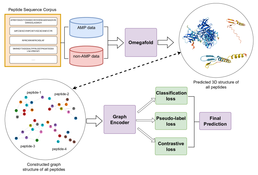
Figure 1: Overall framework of our SGAC model. The framework consists of multiple stages designed to enhance AMP classification. Initially, Omegafold is employed to predict the three-dimensional (3D) structure of peptides based on their amino acid sequences, generating peptide graphs where nodes represent C_α atoms. These graphs are then processed by a Graph Neural Network (GNN) encoder to capture structural and relational features. Then, the embeddings produced by Graph Encoder are refined using three key components: Weight-enhanced Contrastive Learning, which improves feature separation between AMPs and non-AMPs; Weight-enhanced Pseudo-label Distillation, which dynamically refines predictions using high-confidence pseudo labels; and a Classification Loss, which ensures accurate supervised learning by directly optimizing the classification performance. Finally, our SGAC model produce the final prediction results.

The contributions of our paper can be summarized as follows:

• We propose to use Omegafold to predict the 3D spatial structures of peptides, enabling the incorporation of spatial structural information into AMP classification.

• We develop SGAC, which employs GNNs to encode spatial characteristics of each peptide and integrates Weight-enhanced Contrastive Learning and Pseudo-label Distillation to address the class imbalance and improve classification accuracy.

• Experiments on publicly available AMP and non-AMP datasets demonstrate that our SGAC significantly outperforms traditional sequence-based methods and achieves state-of-the-art performance among graph-based models, validating its effectiveness in AMP classification.

2 Methodology

In this paper, we focus on improving the prediction accuracy of AMPs and non-AMPs by leveraging the spatial structural information of peptides. We first predict the 3D structures of peptides based on their amino acid sequences using Omegafold Wu et al. (2022) and construct peptide graphs from the C_α positions of the residues Yim et al. (2023); Liu et al. (2024); Watson et al. (2022). Then, we introduce a novel approach, SGAC, which leverages a Graph Neural Network (GNN) as a Graph Encoder to generate comprehensive peptide representations. To address the class imbalance issue and refine predictions, Weight-enhanced Contrastive Learning clusters similar peptides and separates dissimilar ones by assigning specific weights to positive and negative pairs. Furthermore, Weight-enhanced Pseudo-label Distillation dynamically generates reliable and high confidence pseudo labels, ensuring balanced representation of AMPs and non-AMPs while enforcing consistency with a weighted loss function. The overview of the above process is shown in Figure 1.

2.1 Graph Construction

Let $P=\{a_{1},a_{2},\dots,a_{n}\}$ represents a peptide sequence consisting of $n$ amino acids. The AMP and non-AMP data are initially provided as primary amino acid sequences without atomic-level structural details. To address this limitation, we utilize Omegafold Wu et al. (2022), a pre-trained protein language model that can infer the three-dimensional spatial coordinates of each residue from its amino acid sequence. By leveraging both AMP and non-AMP data by Omegafold, we obtain the corresponding 3D spatial structures for each amino acid residue $a_{i}$. To focus on structural analysis, we only extract the positions of the C_α atoms, which serve as representative spatial coordinates for the amino acid backbone. Such a process will generate a set of 3D coordinates denoted as $\mathbf{R}=\{\mathbf{r}_{1},\mathbf{r}_{2},\dots,\mathbf{r}_{n}\}\in\mathbb{R}^{N\times 3}$, where $\mathbf{r}_{i}\in\mathbb{R}^{3}$ corresponds to the spatial position of the C_α atom for amino acid $a_{i}$.

To represent the peptides as graphs, we use an undirected graph $G=(V,E,\mathbf{X})$ to represent each peptide, where $V$ denotes the set of nodes, $E$ the set of edges, and $\mathbf{X}$ the node feature matrix. The nodes $V$ correspond to the C_α atoms of the amino acids, defined as $V=\{v_{1},v_{2},\dots,v_{n}\}$, with each node $v_{i}$ representing the C_α atom of amino acid $a_{i}$. Edges in the graph are determined based on the Euclidean distances between C_α atoms. Specifically, an edge is established between nodes $v_{i}$ and $v_{j}$ if the distance between their corresponding C_α atoms is less than a predefined threshold $\delta$:

$$E=\left\{\left(v_{i},v_{j}\right)\mid\left\|\mathbf{r}_{i}-\mathbf{r}_{j}\right\|_{2}<\delta,i\neq j\right\},$$ (1)

where $\delta$ controls the connectivity of the graph. The node feature matrix $\mathbf{X}$ encodes the biochemical identity of each amino acid. We produce a comprehensive set of unique amino acid types from the AMP and non-AMP datasets to generate these features. Each amino acid is then represented as a one-hot encoded vector based on its sequence identity, ensuring that the feature matrix $\mathbf{X}$ captures essential sequence-based information.

The constructed graph $G$ captures the spatial relationships between amino acids within the peptide, providing a robust framework for analysing protein structure and function. Additionally, the focus on spatial connectivity through the C_α atoms ensures that the graph $G$ captures essential structural features of each peptide, which are critical for distinguishing AMPs from non-AMPs.

2.2 Graph Encoder

Peptides are intricate biomolecules whose functions are deeply influenced by their structure and spatial relationships. To accurately distinguish AMPs from non-AMPs, we transform the input peptide graphs into graph representations to capture essential structural and relational information within peptides. This approach leverages peptides’ intricate spatial patterns and connectivity to enhance predictive accuracy and biological relevance.

Given a peptide graph $G=(V,E,\mathbf{X})$, we leverage a Graph Neural Network (GNN) to encode its structure and node attributes. Let $\mathbf{h}_{v}^{(l)}$ represent the embedding for node $v$ at the $l$ th layer of the network. The initial embedding $\mathbf{h}_{v}^{(0)}$ is defined by $\mathbf{h}_{v}^{(0)}=\text{MLP}(\mathbf{x}_{v})$, where the MLP$(\cdot)$ is a learnable multi-layer perceptron that maps the node feature $\mathbf{x}_{v}$ into the latent space. Subsequently, for each node $v\in V$, the embedding $\mathbf{h}_{v}^{(l)}$ is updated iteratively through a message-passing framework. At each iteration, the embedding of $v$ is updated by aggregating information from its neighboring nodes $\mathcal{N}(v)$ from the previous layer, and this aggregated information is combined with the embedding of $v$ from the same layer. Formally, this update process is defined as:

$$\mathbf{h}_{v}^{l}=\mathcal{C}^{(l-1)}\left(\mathbf{h}_{v}^{l-1},\mathcal{A}^{(l-1)}\left(\left\{\mathbf{h}_{u}^{l-1}\right\}_{u\in\mathcal{N}(v)}\right)\right),$$ (2)

where $\mathcal{A}^{(l-1)}$ denotes the aggregation operation at the $l-1$-th layer, which aggregates embeddings from the neighbors of $v$, and $\mathcal{C}^{(l-1)}$ represents the combination operation at the $l-1$-th layer, which integrates the aggregated neighbor information with the embedding of $v$ itself. This iterative message-passing mechanism enables the GNN to effectively capture both the local structural interactions among amino acids and the global topology of the peptide graph.

After $L$ layers of iterative updates, a graph-level representation $\mathbf{z}$ is computed for each peptide graph $G$ using a readout function, which aggregates the node representations at the final layer:

$$\mathbf{z}=F\left(G\right)=\operatorname{READOUT}\left(\left\{\mathbf{h}_{v}^{L}\right\}_{v\in\mathcal{V}}\right),$$ (3)

where $\mathbf{z}$ is the graph-level representation for each peptide generated by the GNN function $F(\cdot)$. The $\operatorname{READOUT}$ function can be implemented in various strategies, such as summation, averaging, maximization of node embeddings Xu et al. (2018); Yin et al. (2023a, b) or incorporating a virtual node Li et al. (2015) to capture global graph information. The graph-level representation $\mathbf{z}$ captures the peptide’s structural and relational characteristics, providing a robust foundation for distinguishing AMPs from non-AMPs.

2.3 Weight-enhanced Contrastive Learning

Contrastive learning enhances the discriminative power of feature representations by aligning labeled similar samples while ensuring separation from dissimilar ones Chen et al. (2023); Wang et al. (2023), which is effective for distinguishing AMPs from non-AMPs by capturing their unique structural and relational differences. However, a critical challenge in AMP classification lies in the class imbalance, where non-AMP samples significantly outnumber AMP samples. This imbalance can lead standard contrastive learning methods to overemphasize the majority class (non-AMPs), thereby degrading the model’s ability to classify the minority class (AMPs) accurately.

To address this issue, we introduce Weight-enhanced Contrastive Learning, a tailored approach that incorporates class-specific weights to balance the influence of positive and negative samples during training. By appropriately weighting contributions from each class, this method mitigates the effects of class imbalance, ensuring that the learned representations reflect the distinguishing features of AMPs while maintaining robust discrimination against non-AMPs.

Assuming the Graph Encoder has $L$ message passing layers, we first extract the graph embeddings of the $L$-th layer, where $\mathbf{Z}^{L}=[\mathbf{z}_{1}^{L},\mathbf{z}_{2}^{L},\dots,\mathbf{z}_{|\mathcal{N}_{\text{label}}|}^{L}]^{T}\in\mathbb{R}^{{|\mathcal{N}_{\text{label}}|}\times d}$ for $|\mathcal{N}_{\text{label}}|$ labeled peptide graphs, where $\mathbf{z}_{i}^{L}\in\mathbb{R}^{d}$ is the $d$-dimensional embedding of the $i$-th labeled peptide, and the corresponding label vector $\mathbf{y}=[y_{1},y_{2},\dots,y_{|\mathcal{N}_{\text{label}}|}]$. Contrastive learning aims to optimize embeddings such that peptides sharing the same label are positioned closer together in the latent space. In contrast, those with different labels are pushed further apart. To achieve this, the pairwise Euclidean distance between embeddings is computed as:

$$D_{ij}=\left\|\mathbf{z}_{i}^{L}-\mathbf{z}_{j}^{L}\right\|_{2},\quad\forall i,j\in\{1,2,\ldots,{|\mathcal{N}_{\text{label}}|}\}.$$ (4)

To address the issue of class imbalance, we incorporate class-specific weights, denoted as $\omega_{cl}^{\text{pos}}$ for positive pairs (samples with the same label) and $\omega_{cl}^{\text{neg}}$ for negative pairs (samples with different labels). Specifically, $\omega_{cl}^{\text{pos }}$ is calculated as:

$$\omega_{cl}^{\text{pos}}=1-\frac{\left|\mathcal{N}_{\text{label}}^{\text{pos }}\right|}{\left|\mathcal{N}_{\text{label}}^{\text{pos }}\right|+\left|\mathcal{N}_{\text{label}}^{\text{neg}}\right|},$$ (5)

while $\omega_{cl}^{\text{neg }}$ is calculated by:

$$\omega_{cl}^{\text{neg}}=1-\frac{\left|\mathcal{N}_{\text{label}}^{\text{neg }}\right|}{\left|\mathcal{N}_{\text{label}}^{\text{pos }}\right|+\left|\mathcal{N}_{\text{label}}^{\text{neg }}\right|},$$ (6)

where $\mathcal{N}_{\text{label}}=\mathcal{N}_{\text{label}}^{\text{pos }}+\mathcal{N}_{\text{label}}^{\text{neg}}$, $\mathcal{N}_{\text{label}}^{\text{pos }}$ and $\mathcal{N}_{\text{label}}^{\text{neg }}$ denote the sets of AMP and non-AMP samples in the labeled dataset, respectively, and $\left|\mathcal{N}_{\text{label}}^{\text{pos }}\right|$ and $\left|\mathcal{N}_{\text{label}}^{\text{neg }}\right|$ represent their respective sizes.

These weights ensure that both classes contribute proportionally to the learning process. The positive contrastive loss, which encourages embeddings of peptides with the same label to cluster together, is defined as:

$$\mathcal{L}_{cl}^{\mathrm{pos}}=\omega_{cl}^{\mathrm{pos}}\sum_{i=1}^{|\mathcal{N}_{\text{label}}|}\sum_{j=1}^{|\mathcal{N}_{\text{label}}|} \mathbb{I}\left(y_{i}=y_{j}\right)D_{ij}^{2},$$ (7)

$$\forall i,j\in\left\{1,2,\ldots,\left|\mathcal{N}_{\text{label}}\right|\right\},$$

where $\mathbb{I}(\cdot)$ is an indicator function that equals 1 if $y_{i}=y_{j}$, and 0 otherwise. This formulation allows for the effective integration of class-specific contributions, improving the model’s ability to capture the intrinsic relationships within the peptide data, even when the class distribution is imbalanced.

To ensure sufficient separation between embeddings of peptides with different labels, we apply a margin $m$ for negative pairs. This margin enforces a minimum distance between dissimilar samples, thereby enhancing the discriminative power of the model. The negative contrastive loss is defined as:

$$\mathcal{L}_{cl}^{\mathrm{neg}}=\omega_{cl}^{\mathrm{neg}}\sum_{i=1}^{|\mathcal{N}_{\text{label}}|}\sum_{j=1}^{|\mathcal{N}_{\text{label}}|}\mathbb{I} \left(y_{i}\neq y_{j}\right)\max\left(0,m-D_{ij}\right)^{2},$$ (8)

$$\forall i,j\in\left\{1,2,\ldots,\left|\mathcal{N}_{\text{label}}\right|\right\},$$

where $\mathbb{I}\left(y_{i}\neq y_{j}\right)$ is an indicator function that equals 1 if $y_{i}\neq y_{j}$ and 0 otherwise. The term $\max\left(0,m-D_{ij}\right)$ ensures that negative pairs contribute to the loss only when their distance $D_{ij}$ is less than the margin $m$.

Finally, the overall Weight-enhanced Contrastive Loss, $\mathcal{L}_{\text{cl}}$, combines the positive and negative losses, normalized by the total number of sample pairs to account for the dataset size, which is defined as follows:

$$\mathcal{L}_{\text{cl}}=\frac{1}{|\mathcal{N}_{\text{label}}|*(|\mathcal{N}_{\text{label}}|-1)}\left(\mathcal{L}_{cl}^{\mathrm{pos}}+\mathcal{L}_{cl}^{\mathrm{neg}}\right).$$ (9)

This formulation ensures a balanced optimization of embeddings, effectively leveraging both positive and negative pairs while mitigating the effects of class imbalance.

2.4 Weight-enhanced Pseudo Label Distillation

Pseudo-label learning leverages unlabeled data by assigning high-confidence pseudo-labels to enable iterative refinement of the model’s understanding of the data distribution. This process ensures semantic consistency across different latent spaces and is particularly useful for addressing the scarcity of labeled AMP data while facilitating the discovery of novel AMP sequences. However, traditional pseudo-label distillation methods often suffer from the inherent class imbalance between AMP and non-AMP samples, resulting in model bias toward the majority class.

To address this issue, we propose Weight-Enhanced Pseudo-Label Distillation, a method designed to dynamically balance the contributions of AMP and non-AMP samples while aligning semantic information between labeled and unlabeled data. Additionally, this method incorporates soft-label refinement to produce accurate peptide representations, effectively mitigating the impact of class imbalance.

Assuming the Graph Encoder consists of $L$ message-passing layers, we produce pseudo-labels for unlabeled peptides using the embeddings generated from the $l$-th hidden layer. These embeddings are represented as $\mathbf{Z}^{l}=\left[\mathbf{z}_{1}^{l},\mathbf{z}_{2}^{l},\ldots,\left.\mathbf{z}_{\left|\mathcal{N}_{\text{unlabel }}\right|}^{l}\right|^{T}\in\mathbb{R}^{\left|\mathcal{N}_{\text{unlabel}}\right|\times d}\right.$, where $\left|\mathcal{N}_{\text{unlabel}}\right|$ denotes the number of unlabeled peptide graphs, and $\mathbf{z}_{i}^{l}\in\mathbb{R}^{d}$ is the $d$-dimensional embedding of the $i$-th unlabeled peptide.

We cluster these peptide embeddings into $K$ clusters using the K-Means algorithm Hartigan et al. (1979). The initial cluster centers are denoted as $\mathbf{C}=\left\{\mathbf{c}_{1},\mathbf{c}_{2},\ldots,\mathbf{c}_{K}\right\}\in\mathbb{R}^{K\times d}$. The pairwise distance $V_{ij}$ between the $i$-th peptide embedding $\mathbf{z}_{i}^{l}$ and the $j$-th cluster center $\mathbf{c}_{j}$ is computed as:

$$V_{ij} =\left\|\mathbf{z}_{i}^{l}-\mathbf{c}_{j}\right\|_{2},$$ (10)

$$\quad\forall i\in\left\{1,2,\ldots,\left|\mathcal{N}_{\text{unlabel}}\right|\right\},$$

$$\quad\forall j\in\{1,2,\ldots,K\},$$

where $V_{ij}$ denotes the Euclidean distance between $\mathbf{z}_{i}^{l}$ and $\mathbf{c}_{j}$. Then, the distances are then converted into probabilities using a softmax function:

$$p_{ij}=\frac{\exp\left(-V_{ij}\right)}{\sum_{n=1}^{K}\exp\left(-V_{in}\right)}.$$ (11)

Finally, the pseudo-label $\hat{y}_{i}$ for $i$-th unlabeled peptide is assigned to the class with the highest probability:

$$\hat{y}_{i}=\arg\max_{j}p_{ij}.$$ (12)

Moreover, to emphasize high-confidence predictions, we define the associated confidence score for each unlabeled peptide. In details, for $i$-th unlabeled peptide, the confidence score $s_{i}$ is calculated as

$$s_{i}=\max_{j}p_{ij},$$ (13)

which can reflect the model’s certainty in its prediction. We then construct the confident sets for the unlabeled peptides based on their pseudo labels and confidence scores as follows:

$$\mathcal{N}_{\mathrm{c}}^{\text{pos }} =\left\{i\mid\hat{y}_{i}=1,s_{i}>\tau\right\}$$ (14)

$$\mathcal{N}_{\mathrm{c}}^{\text{neg }} =\left\{j\mid\hat{y}_{j}=0,s_{j}>\tau\right\},$$

$$\forall i,j\in\left\{1,2,\ldots,\left|\mathcal{N}_{\text{unlabel}}\right|\right\},$$

where $\mathcal{N}_{\mathrm{c}}^{\text{pos }}$ represents the confident set of peptides with the pseudo label $\hat{y}=1$, and $\mathcal{N}_{\mathrm{c}}^{\text{neg }}$ represents the confident set of peptides with the pseudo label $\hat{y}=0$. Here, $\tau$ is a predefined threshold value, which is set to 0.5 for convenience. These confident sets form the foundation for further training and refinement in the AMP classification task.

For further adapting to evolving embedding distributions, the cluster centers are updated based on mean embeddings of the confident samples assigned to each cluster. For cluster $j$, the new cluster center $\mathbf{\hat{c}}_{j}$ is computed as:

$$\mathbf{\hat{c}}_{j}=\frac{1}{\left|\mathcal{N}_{c}^{j}\right|} \sum_{i\in\mathcal{N}_{c}^{j}}\mathbf{z}_{i}^{l},$$ (15)

$$\forall j\in\{\text{pos},\text{neg}\},$$

where $\mathcal{N}^{j}_{c}$ is the set of confident samples assigned to cluster $j$, $|\mathcal{N}^{j}_{c}|$ is the size of $\mathcal{N}^{j}_{c}$.

Next, to mitigate the class imbalance inherent in AMP and non-AMP data, class-specific weights are introduced, which are denoted as $\omega_{cl}^{\text{pos}}$ for AMP data and $\omega_{cl}^{\text{neg}}$ for non-AMP data. Specifically, $\omega_{pl}^{\text{pos }}$ is calculated as:

$$\omega_{pl}^{\text{pos }}=1-\frac{\left|\mathcal{N}_{\text{c}}^{\text{pos }}\right|}{\left|\mathcal{N}_{\text{c}}^{\text{pos }}\right|+\left|\mathcal{N}_{\text{c}}^{\text{neg }}\right|},$$ (16)

similarly, $\omega_{pl}^{\text{neg }}$ is calculated by:

$$\omega_{pl}^{\text{neg}}=1-\frac{\left|\mathcal{N}_{\text{c}}^{\text{neg }}\right|}{\left|\mathcal{N}_{\text{c}}^{\text{pos }}\right|+\left|\mathcal{N}_{\text{c}}^{\text{neg }}\right|}.$$ (17)

The positive pseudo label loss, $\mathcal{L}^{\text{pos}}_{pl}$, is calculated as:

$$\mathcal{L}_{pl}^{\mathrm{pos}}=\omega_{pl}^{\mathrm{pos}}\frac{1}{|\mathcal{N}_{c}^{\text{pos}}|}\sum_{i\in\mathcal{N}_{c}^{\text{pos}}}-\log\left(p_{i,\hat{y}=1}\right),$$ (18)

where $p_{i,\hat{y}=1}$ denotes the predicted probability of the $i$-th unlabeled peptides in $\mathcal{N}_{c}^{\text{pos}}$. Conversely, the negative pseudo label loss, $\mathcal{L}_{pl}^{\text{neg}}$, is expressed as:

$$\mathcal{L}_{pl}^{\text{neg }}=\omega_{pl}^{\text{neg }}\frac{1}{|\mathcal{N}_{c}^{\text{neg}}|}\sum_{j\in\mathcal{N}_{c}^{\text{neg}}}-\log\left(p_{j,\hat{y}=0}\right),$$ (19)

where $p_{j,\hat{y}=0}$ is the predicted probability of the $j$-th unlabeled peptides in $\mathcal{N}_{c}^{\text{neg}}$.

Furthermore, a soft-label refinement loss is introduced using Kullback-Leibler (KL) divergence to refine pseudo-labels and maintain consistency across different layers of Graph Encoder. The soft-label refinement loss is defined as:

$$\mathcal{L}_{\mathrm{soft}}=\alpha\frac{1}{\left|\mathcal{N}_{\mathrm{c}}\right|}\sum_{i=1}^{\left|\mathcal{N}_{\mathrm{c}}\right|}\sum_{j=1}^{K}{p}_{ij}\log\left(\frac{{p}_{ij}}{\hat{p}_{ij}}\right),$$ (20)

where $\mathcal{N}_{\text{c}}=\mathcal{N}_{\text{c}}^{\text{pos}}\cup\mathcal{N}_{\text{c}}^{\text{neg}}$, $|\mathcal{N}_{\text{c}}|$ is the size of $\mathcal{N}_{\text{c}}$, ${p}_{ij}$ is the probability of the $i$-th unlabeled peptides belonging to class $j$ from layer $l$, $\hat{p}_{ij}$ is the predicted probability of the $i$-th unlabeled peptides belonging to class $j$ from layer $L$, and $\alpha=1-\bar{c}$ is a dynamic weighting factor influenced by the mean confidence, which is defined as

$$\bar{c}=\frac{1}{\left|\mathcal{N}_{\mathrm{c}}\right|}\sum_{i=1}^{\left|\mathcal{N}_{\mathrm{c}}\right|}\max_{j}p_{ij}.$$ (21)

The overall Weight-enhanced Pseudo-label loss, $\mathcal{L}_{\mathrm{pl}}$, integrates the above three components:

$$\mathcal{L}_{\text{pl}}=\mathcal{L}_{pl}^{\text{pos }}+\mathcal{L}_{pl}^{\text{neg }}+\mathcal{L}_{\text{soft }}.$$ (22)

This composite loss ensures balanced pseudo-label learning, aligning the model’s predictions with true distributions while addressing class imbalances and refining pseudo-label accuracy.

2.5 Learning Framework

To ensure effective learning from supervised data, we minimize the expected error for labeled data using a classification loss. Assuming the Graph encoder has $L$ message passing layers, we extract the embeddings of the final layer, where $\mathbf{Z}^{L}=[\mathbf{z}_{1}^{L},\mathbf{z}_{2}^{L},\dots,\mathbf{z}_{|\mathcal{N}_{\text{label}}|}^{L}]^{T}\in\mathbb{R}^{{|\mathcal{N}_{\text{label}}|}\times d}$ for $|\mathcal{N}_{\text{label}}|$ labeled peptide graphs, where $\mathbf{z}_{i}^{L}\in\mathbb{R}^{d}$ is the $d$-dimensional embedding of the $i$-th peptides, and the corresponding label vector $\mathbf{y}=[y_{1},y_{2},\dots,y_{|\mathcal{N}_{\text{label}}|}]$. The classification loss is defined as:

$$\mathcal{L}_{\text{cf}}=\frac{1}{|\mathcal{N}_{\text{label}}|}\sum_{i=1}^{|\mathcal{N}_{\text{label}}|}\text{CE}(\operatorname{MLP}(\mathbf{z}^{L}_{i}),y_{i}),$$ (23)

where MLP $(\cdot)$ is a multi-layer perceptron that maps the protein embedding $\mathbf{z}^{L}_{i}$ to the predicted label space, and $\text{CE}(\cdot,\cdot)$ represents the cross-entropy loss function.

Finally, the overall training objective of SGAC combines the classification loss $\mathcal{L}_{\mathrm{cf}}$, the Weight-enhanced Contrastive Learning loss $\mathcal{L}_{\mathrm{cl}}$ and the Weight-enhanced Pseudo-label loss $\mathcal{L}_{\text{pl }}$, which is formulated as follows:

$$\mathcal{L}=\mathcal{L}_{\text{cf}}+\lambda\mathcal{L}_{\text{cl}}+\gamma\mathcal{L}_{\text{pl}},$$ (24)

where $\lambda$ and $\gamma$ are hyperparameters that balance the ratio of the Weight-enhanced Contrastive Learning loss and the Weight-enhanced Pseudo-label loss relative to the classification loss. These components enable our SGAC to effectively integrate labeled data, structural information, and pseudo-labeled samples, ensuring robust and balanced learning for AMP and non-AMP classification.

2.6 AMP Prediction

In the final stage of our framework, we predict whether a given peptide sequence belongs to the AMP class or the non-AMP class based on the learned graph representations. The AMP prediction process leverages the comprehensive features captured by the Graph Encoder, as well as the refinements provided by Weight-enhanced Contrastive Learning and Weight-enhanced Pseudo-label Distillation.

Given the graph-level representation $\mathbf{z}_{i}$ of $i$-th peptide graph generated by the Graph Encoder, we employ a Multi-Layer Perceptron (MLP) for classification. Specifically, the prediction probability $p_{ij}$ is computed as:

$$p_{ij}=\mathrm{softmax}(\mathrm{MLP}(\mathbf{z}_{i})),$$ (25)

where the MLP $(\cdot)$ maps the graph representation $\mathbf{z}_{i}$ to a probability distribution over the AMP and non-AMP classes.

The final classification decision for $i$-th peptide is determined by:

$$\overline{y}_{i}=\arg\max_{j}p_{ij},$$ (26)

where $\overline{y}_{i}$ is the predicted label for the $i$-th peptide.

Table 1: Statistics of the AMP and non-AMP datasets, which presents the number of graphs, average nodes, and average edges for the complete dataset, as well as for AMPs and non-AMPs separately.

Datasets	Graphs	Avg. Nodes	Avg. Edges	Classes
AMPs & non-AMPs	65,971	38.8	195.8	2
AMPs	7,697	23.1	118.6	2
non-AMPs	58,274	40.9	206.1	2

3 Experiments

In this section, we conduct extensive experiments to verify the effectiveness of SGAC in AMP and non-AMP classification task.

3.1 Experimental settings

Dataset. The AMP data was sourced from the DRAMP database Ma et al. (2024), which provides detailed annotations of antimicrobial peptides, while the non-AMP data was obtained from Ma et al. (2022). To ensure consistency, both AMP and non-AMP sequences were filtered to include only peptides with lengths ranging from 10 to 50 amino acids Jha et al. (2022); Wang et al. (2022). Following the graph construction methodology described in Section 2.1, these amino acid sequences are transformed into graphs using their predicted 3D structures derived from amino acid sequences. The statistics of the processed datasets are presented in Table 1.

Baselines. To validate the effectiveness of converting amino acid sequence structures into graph structures and demonstrate the performance of SGAC, we compare two categories of methods: (1) four widely used sequence-based models, including BERT (Devlin, 2018), Attention (Vaswani, 2017), LSTM (Hochreiter, 1997), Random Forest (Breiman, 2001), and Diff-AMP Wang et al. (2024a); and (2) three widely used graph neural networks (GNNs), namely GCN (Kipf and Welling, 2016), GIN (Xu et al., 2018), and GraphSAGE (Hamilton et al., 2017).

Evaluation metrics. To comprehensively evaluate the performance of SGAC, we employ three widely used metrics: F1 score, Area Under the Receiver Operating Characteristic Curve (AUC), and Precision-Recall Area Under the Curve (PR-AUC). These metrics evaluate the model’s predictive capability, especially for tasks with imbalanced datasets.

• The F1 score is a harmonic mean of precision and recall, which evaluates the balance between false positives and false negatives. It is particularly effective in imbalanced datasets and computed as follows:

  $$\mathrm{Precision}=\frac{\mathrm{True\ Positive}}{\mathrm{True\ Positive}+\mathrm{False\ Positive}},$$ (27)

  $$\mathrm{Recall}=\frac{\mathrm{True\ Positive}}{\mathrm{True\ Positive}+\mathrm{False\ Negative}},$$ (28)

  $$\mathrm{F1\ Score}=\frac{2\times\mathrm{Precision}\times\mathrm{Recall}}{\mathrm{Precision}+\mathrm{Recall}}.$$ (29)

  A higher F1 score indicates better overall model performance.

• AUC measures the performance of a binary classifier by analyzing the relationship between the True Positive Rate (TPR) and the False Positive Rate (FPR) at varying thresholds. TPR and FPR are defined as:

  $$\mathrm{TPR}=\frac{\mathrm{True\ Positive}}{\mathrm{True\ Positive}+\mathrm{False\ Negative}},$$ (30)

  $$\mathrm{FPR}=\frac{\mathrm{False\ Positive}}{\mathrm{False\ Positive}+\mathrm{True\ Negative}}.$$ (31)

  The Receiver Operating Characteristic (ROC) curve plots TPR against FPR at different thresholds. AUC is the area under the ROC curve, which summarizes the classifier’s overall performance. Higher AUC values indicate superior classification performance and better discrimination between classes.

• PR-AUC is a metric that evaluates the relationship between precision and recall across different thresholds, emphasizing performance on imbalanced datasets. It is calculated as the area under the precision-recall curve. Especially, PR-AUC is particularly useful for tasks with imbalanced datasets, as it focuses on the model’s performance in predicting the minority class. Higher PR-AUC values indicate better precision-recall trade-offs.

Table 2: Performance comparison among baselines and SGAC. Bold results indicate the best performance.

Method	F1	AUC	PR-AUC
BERT	21.95	50.00	55.85
Diff-AMP	36.36	69.87	56.33
LSTM	45.40	79.79	58.37
Attention	86.70	89.55	88.56
Random Forest	87.97	97.96	93.86
GCN	88.18 $\pm$ 0.81	99.01 $\pm$ 0.02	95.57 $\pm$ 0.10
GraphSAGE	91.26 $\pm$ 0.42	99.26 $\pm$ 0.05	96.00 $\pm$ 0.12
GIN	92.61 $\pm$ 0.81	99.13 $\pm$ 0.03	96.73 $\pm$ 0.20
SGAC	95.13 $\pm$ 0.46	99.64 $\pm$ 0.04	98.45 $\pm$ 0.09

Table 3: The performance of SGAC with different GNN architectures. Bold results indicate the best performance.

Method	F1	AUC	PR-AUC
SGAC w GCN	93.75 $\pm$ 0.47	99.31 $\pm$ 0.09	97.88 $\pm$ 0.17
SGAC w GraphSAGE	94.03 $\pm$ 0.24	99.44 $\pm$ 0.10	98.17 $\pm$ 0.12
SGAC w GIN	95.13 $\pm$ 0.46	99.64 $\pm$ 0.04	98.45 $\pm$ 0.09

Implementation details. SGAC, GNN baselines and BERT are implemented using PyTorch, while LSTM, Attention, and Random Forest are implemented using scikit-learn. For SGAC, we use GIN (Xu et al., 2018) as the backbone for the Graph Encoder introduced in Section 2.2, incorporating a mean-pooling layer as the readout function. All experiments for SGAC and baselines are conducted on NVIDIA A100 GPUs to ensure a fair comparison, where the learning rate of Adam optimizer is set to ${10^{-4}}$, hidden embedding dimension 256, weight decay ${10^{-12}}$, and GNN layers 4. For sequence-based models such as BERT, Attention, LSTM, and Diff-AMP, we use pre-trained model weights from Ma et al. (2022) and Wang et al. (2024a) for predictions, respectively. In contrast, Random Forest and GNNs, including GCN, GIN, and GraphSAGE, are trained from scratch for this evaluation. The performances of all GNN models are measured and averaged on all samples for five runs.

3.2 Performance comparisons

We present the results of the proposed SGAC and all baselines in Table 2. We can observe that (1) Random Forest demonstrates the highest performance among sequence-based methods, indicating its strong capability in extracting informative features from amino acid sequences. Nevertheless, it remains inferior to graph-based models, which emphasize the limitations of sequence-based methods in capturing the structural and relational information inherent in proteins. (2) Graph-based methods are superior to sequence-based approaches, highlighting the effectiveness of representing proteins as graph structures. Among GNNs, GIN achieves the highest performance and outperforms both GCN and GraphSAGE. This result demonstrates the ability of GNNs to effectively capture structural and relational information from graph representations of amino acid sequences. (3) SGAC outperforms all baselines across all evaluation metrics, demonstrating its superiority in AMP classification. Specifically, it achieves a relative gain of 2.52% in F1 score, 0.51% in AUC, and 1.72% in PR-AUC over GIN, emphasizing the effectiveness of its design. The superior performance of SGAC can be attributed to two core components: the Weight-enhanced Contrastive Learning module, which addresses class imbalance by balancing the contributions of AMP and non-AMP samples, and the Weight-enhanced Pseudo-label Distillation module, which dynamically refines pseudo-labels to produce balanced and accurate representations. Therefore, these modules enable SGAC to effectively capture structural and relational information of AMPs and non-AMPs, particularly in scenarios with imbalanced datasets.

We further evaluate the flexibility of the proposed SGAC by replacing different GNN architectures as the backbone of the Graph Encoder. Specifically, GIN is replaced with GCN and GraphSAGE, and the corresponding performance results are presented in Table 3. The results demonstrate that SGAC w GIN consistently achieves the best performance across all metrics. This superior performance underscores GIN’s strong representational capacity, enabling it to effectively capture the structural and relational characteristics of graph-structured data. This phenomenon also justifies using GIN as the backbone of Graph Encoder to enhance the proposed SGAC performance.

Table 4: The results of ablation studies. Bold results indicate the best performance per column.

Method	F1	AUC	PR-AUC
SGAC w/o cf	78.67	92.76	80.90
SGAC w/o pl	94.57	99.47	98.31
SGAC w/o cl	94.62	99.50	98.35
SGAC	95.13	99.64	98.45

3.3 Ablation study

We conduct ablation studies to examine the contributions of each component in the proposed SGAC: (1) SGAC w/o cf: It removes the classification loss $\mathcal{L}_{cf}$; (2) SGAC w/o cl: It removes the Weight-enhanced Contrastive Learning loss $\mathcal{L}_{cl}$ ; (3) SGAC w/o pl: It removes the Weight-enhanced Pseudo-label loss $\mathcal{L}_{pl}$.

Experimental results are shown in Table 4. From the table, we find that (1) SGAC outperforms SGAC w/o cf, SGAC w/o pl, and SGAC w/o cl across all evaluation metrics, demonstrating the critical contributions of each component to the overall performance. (2) SGAC w/o cf shows lower performance compared to SGAC, showing that $\mathcal{L}_{cf}$ is crucial in leveraging labeled data effectively. This result also indicates that $\mathcal{L}_{cf}$ is crucial in guiding the model to learn meaningful and robust graph representations. (3) The SGAC w/o pl model performs worse than SGAC, validating the significance of the Weight-enhanced Pseudo Label Distillation module. The iterative refinement of pseudo-labels enables SGAC to maintain balanced and robust feature representations. (4) SGAC is superior to SGAC w/o cl, demonstrating the importance of Weight-enhanced Contrastive Learning in balancing the contributions of AMP and non-AMP samples during training. This balance effectively enhances representation quality and addresses class imbalance.

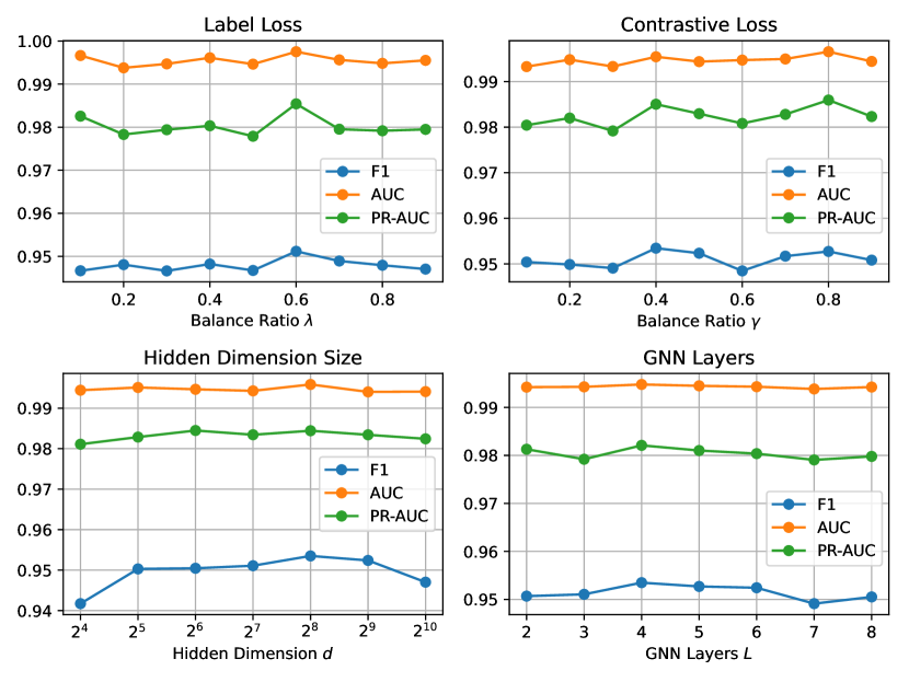
Figure 2: Hyper-parameter sensitivity analysis of $\lambda$, $\gamma$, Hidden dimension size $d$ and GNN layers $L$.

3.4 Sensitivity Analysis

We study the sensitivity analysis of SGAC with respect to the impact of its hyperparameters: balance ratio $\lambda$ and $\gamma$, hidden dimension size $d$, and GNN layers $L$, which plays a crucial role in the performance of SGAC. Especially, $\lambda$ and $\gamma$ control the relative contributions of $\mathcal{L}_{\text{cl}}$ and $\mathcal{L}_{\text{pl}}$ to the overall objective, ensuring practical trade-offs between classification, contrastive learning, and pseudo-label distillation; $d$ determines the dimension of the learned graph representations, which directly impacts the model’s capacity to capture structural and relational information; $L$ governs the depth of message passing in the GNNs, which influences the ability to aggregate information from neighbors and model higher-order relationships in the graph.

Figure 2 illustrates how $\lambda$, $\gamma$, $d$ and $L$ affects the performance of SGAC. We vary $\lambda$ and $\gamma$ within the range of $\{0.1,0.2,0.3,0.4,0.5,0.6,0.7,0.8,0.9\}$, $d$ in $\{2^{4},2^{5},2^{6},2^{7},2^{8},2^{9},2^{10}\}$, and $L$ in $\{2,3,4,5,6,7,8\}$. From the results, we observe that: (1) The performance of SGAC in Figure 2 generally stabilizes across a wide range of $\lambda$ values and $\gamma$ values. The slight variations in the F1 score indicate a potential trade-off among the contributions of $\mathcal{L}_{cf}$, $\mathcal{L}_{cl}$ and $\mathcal{L}_{pl}$. SGAC achieves optimal performance around $\lambda=0.6$ and $\gamma=0.4$, which is chosen as the default setting. (2) The performance of SGAC improves, as $d$ increases from $2^{4}$ to $2^{8}$, peaking at $d=2^{8}$. Then, the F1 score slightly declines, while AUC and PR-AUC plateau. This indicates that larger dimensions may introduce overfitting or unnecessary complexity without yielding substantial performance improvements. Therefore, $d=2^{8}$ is selected as the optimal hidden dimension size. (3) The performance of SGAC improves and then keeps stable as $L$ increases from 2 to 6, demonstrating that deeper architectures effectively capture structural information of protein graphs. However, when $L>6$, the model performance slightly drops due to over-smoothing. $L=4$ is selected as the default value to balance performance and computational efficiency.

Table 5: Statistics of the dataset used in the case study, showing the number of graphs, average nodes, and average edges for AMPs, non-AMPs, and their combined dataset.

Datasets	Graphs	Avg. Nodes	Avg. Edges	Classes
AMPs & non-AMPs	78	23.1	51.7	2
AMPs	55	23.3	52.3	2
non-AMPs	23	22.5	50.1	2

3.5 Case study

To test the practicality of SGAC, we conducted a case study utilizing the potential antimicrobial peptide data synthesized in Torres et al. (2024). They utilized MetaProdigal to identify 444,000 small open reading frames (smORFs) from 1,773 human microbiome metagenomes. Subsequently, they utilized AmPEP, a random forest classifier, to predict the antimicrobial activity of these smORFs, resulting in 323 smORF-encoded candidate antimicrobial peptides (SEPs). Through a series of selection criteria, they selected 78 high-priority antimicrobial peptides for synthesis and experimental validation. The vitro experiments indicate that 70.5% (55/78) of the synthesized SEPs exhibited antimicrobial activity against at least one pathogen. Following the preprocessing methodology detailed in Section 2.1, graphs are constructed for these peptides, where the statistics of these graphs are summarized in Table 5. These peptide graphs are then input into the trained SGAC model for inference. The experimental results show that SGAC accurately classified 40 of the true AMPs and 5 of the non-AMPs.

For this outcome, we have the following analysis: (1) The distributional characteristics of these peptide graphs help explain the prediction results of SGAC. Specifically, these samples were initially selected due to their high sequence similarity to known AMPs, resulting in intrinsic similarities between the 55 confirmed AMPs and the 23 non-AMPs. Consequently, their underlying graph structures, comprising nodes, edges, and spatial relationships, are not sufficiently distinct. This significant structural overlap introduces ambiguity in the learned representations, making it challenging for the model to confidently distinguish between AMPs and non-AMPs. (2) The distribution of these peptide graphs in the latent space learned by SGAC likely forms clusters where non-AMPs are positioned close to AMPs due to their similar biochemical properties. The weight-enhanced contrastive learning and pseudo-label distillation mechanisms in SGAC are designed to mitigate these challenges by promoting the separation between AMP and non-AMP samples. However, when non-AMPs exhibit structural patterns that closely resemble those of AMPs, the model’s ability to discriminate between the two classes becomes limited, resulting in misclassifications. (3) The limited dataset size and the class imbalance inherent in this AMP classification task increase the difficulty distinguishing these samples. Although SGAC can effectively mitigate the class imbalance issue during training, its generalization ability is hindered when confronted with ambiguous samples. The observed misclassifications arise from these borderline cases, where the model struggles to capture subtle differences between AMPs and non-AMPs within the latent space.

4 Conclusion

In this study, we introduced the Spatial GNN-based AMP Classifier (SGAC), a novel framework for distinguishing AMPs from non-AMPs using the spatial structural information of peptides. Our approach mitigates two significant challenges in AMP classification: the limited availability of labeled AMP data and the inherent class imbalance.

By incorporating three-dimensional peptide structures predicted by Omegafold, SGAC constructs graph representations that capture essential structural and relational characteristics of peptides. The graph encoder, based on Graph Neural Networks (GNNs), effectively extracts these features for classification. To enhance performance and mitigate class imbalance, we integrated Weight-enhanced Contrastive Learning and Weight-enhanced Pseudo-label Distillation into the SGAC framework. Contrastive learning improves the discriminative power by clustering similar peptides while separating dissimilar ones, whereas pseudo-label distillation refines predictions and dynamically incorporates high-confidence unlabeled data. The combined effect of these components ensures balanced representation learning and robust classification performance.

Experimental results on publicly available AMP and non-AMP datasets demonstrate that GNN-based methods significantly outperforms traditional sequence-based methods and SGAC achieves state-of-the-art performance among all baselines. The ablation study and sensitivity analysis validate the contributions of each component, emphasizing the importance of incorporating spatial information and addressing class imbalance. The case study on a biosynthetic dataset of potential antimicrobial peptides has demonstrated the superior practicality of our SGAC in the process of antimicrobial peptide discovery. Therefore, this work advances the field of AMP classification, offering a powerful tool for accelerating the discovery of novel antimicrobial peptides and supporting drug discovery efforts in the face of rising antibiotic resistance.

For future work, we plan to explore the integration of advanced geometric deep learning techniques to capture higher-order structural relationships within peptides. Additionally, expanding the dataset with experimentally verified AMPs and non-AMPs will further improve model generalization. Incorporating domain-specific knowledge, such as functional annotations or physicochemical properties, may also enhance the discriminative power of the classifier. Finally, applying the framework to other peptide-related tasks, such as protein-protein interaction prediction and peptide-drug binding analysis, represents promising directions for future research.

References

- Arakal et al. [2023] Benita S Arakal, David E Whitworth, Philip E James, Richard Rowlands, Neethu PT Madhusoodanan, Malvika R Baijoo, and Paul G Livingstone. In silico and in vitro analyses reveal promising antimicrobial peptides from myxobacteria. Probiotics and Antimicrobial Proteins, 15(1):202–214, 2023.
- Bhadra et al. [2018] Pratiti Bhadra, Jielu Yan, Jinyan Li, Simon Fong, and Shirley WI Siu. Ampep: Sequence-based prediction of antimicrobial peptides using distribution patterns of amino acid properties and random forest. Scientific reports, 8(1):1697, 2018.
- Breiman [2001] Leo Breiman. Random forests. Machine learning, 45:5–32, 2001.
- Chen et al. [2023] Xiaoru Chen, Yingxu Wang, Jinyuan Fang, Zaiqiao Meng, and Shangsong Liang. Heterogeneous graph contrastive learning with metapath-based augmentations. IEEE Transactions on Emerging Topics in Computational Intelligence, 2023.
- Couso and Patraquim [2017] Juan-Pablo Couso and Pedro Patraquim. Classification and function of small open reading frames. Nature reviews Molecular cell biology, 18(9):575–589, 2017.
- Cui et al. [2024] Meili Cui, Mengyue Wang, Xia Liu, Haoyan Sun, Zhenghua Su, Yu Zheng, Yanbing Shen, and Min Wang. Mining and characterization of novel antimicrobial peptides from the large-scale microbiome of shanxi aged vinegar based on metagenomics, molecular dynamics simulations and mechanism validation. Food Chemistry, 460:140646, 2024.
- Devlin [2018] Jacob Devlin. Bert: Pre-training of deep bidirectional transformers for language understanding. arXiv preprint arXiv:1810.04805, 2018.
- Durrant and Bhatt [2021] Matthew G Durrant and Ami S Bhatt. Automated prediction and annotation of small open reading frames in microbial genomes. Cell host & microbe, 29(1):121–131, 2021.
- Fu et al. [2012] Limin Fu, Beifang Niu, Zhengwei Zhu, Sitao Wu, and Weizhong Li. Cd-hit: accelerated for clustering the next-generation sequencing data. Bioinformatics, 28(23):3150–3152, 2012.
- Hamilton et al. [2017] Will Hamilton, Zhitao Ying, and Jure Leskovec. Inductive representation learning on large graphs. Advances in neural information processing systems, 30, 2017.
- Hartigan et al. [1979] John A Hartigan, Manchek A Wong, et al. A k-means clustering algorithm. Applied statistics, 28(1):100–108, 1979.
- Hochreiter [1997] S Hochreiter. Long short-term memory. Neural Computation MIT-Press, 1997.
- Huang et al. [2023] Junjie Huang, Yanchao Xu, Yunfan Xue, Yue Huang, Xu Li, Xiaohui Chen, Yao Xu, Dongxiang Zhang, Peng Zhang, Junbo Zhao, et al. Identification of potent antimicrobial peptides via a machine-learning pipeline that mines the entire space of peptide sequences. Nature Biomedical Engineering, 7(6):797–810, 2023.
- Hyatt et al. [2012] Doug Hyatt, Philip F LoCascio, Loren J Hauser, and Edward C Uberbacher. Gene and translation initiation site prediction in metagenomic sequences. Bioinformatics, 28(17):2223–2230, 2012.
- Jha et al. [2022] Kanchan Jha, Sriparna Saha, and Hiteshi Singh. Prediction of protein–protein interaction using graph neural networks. Scientific Reports, 12(1):8360, 2022.
- Kipf and Welling [2016] Thomas N Kipf and Max Welling. Semi-supervised classification with graph convolutional networks. arXiv preprint arXiv:1609.02907, 2016.
- Kumar et al. [2024] Naveen Kumar, Prashant Bhagwat, Suren Singh, and Santhosh Pillai. A review on the diversity of antimicrobial peptides and genome mining strategies for their prediction. Biochimie, 2024.
- Lata et al. [2007] Sneh Lata, BK Sharma, and Gajendra PS Raghava. Analysis and prediction of antibacterial peptides. BMC bioinformatics, 8:1–10, 2007.
- Lata et al. [2010] Sneh Lata, Nitish K Mishra, and Gajendra PS Raghava. Antibp2: improved version of antibacterial peptide prediction. BMC bioinformatics, 11:1–7, 2010.
- Li et al. [2015] Yujia Li, Daniel Tarlow, Marc Brockschmidt, and Richard Zemel. Gated graph sequence neural networks. arXiv preprint arXiv:1511.05493, 2015.
- Liu et al. [2024] Ce Liu, Jun Wang, Zhiqiang Cai, Yingxu Wang, Huizhen Kuang, Kaihui Cheng, Liwei Zhang, Qingkun Su, Yining Tang, Fenglei Cao, et al. Dynamic pdb: A new dataset and a se (3) model extension by integrating dynamic behaviors and physical properties in protein structures. arXiv preprint arXiv:2408.12413, 2024.
- Liu et al. [2022] Licheng Liu, Caiyun Wang, Mengyue Zhang, Zixuan Zhang, Yingying Wu, and Yixuan Zhang. An efficient evaluation system accelerates -helical antimicrobial peptide discovery and its application to global human genome mining. Frontiers in Microbiology, 13:870361, 2022.
- Ma et al. [2024] Tianyue Ma, Yanchao Liu, Bingxin Yu, Xin Sun, Huiyuan Yao, Chen Hao, Jianhui Li, Maryam Nawaz, Xun Jiang, Xingzhen Lao, et al. Dramp 4.0: an open-access data repository dedicated to the clinical translation of antimicrobial peptides. Nucleic Acids Research, page gkae1046, 2024.
- Ma et al. [2022] Yue Ma, Zhengyan Guo, Binbin Xia, Yuwei Zhang, Xiaolin Liu, Ying Yu, Na Tang, Xiaomei Tong, Min Wang, Xin Ye, et al. Identification of antimicrobial peptides from the human gut microbiome using deep learning. Nature Biotechnology, 40(6):921–931, 2022.
- Magana et al. [2020] Maria Magana, Muthuirulan Pushpanathan, Ana L Santos, Leon Leanse, Michael Fernandez, Anastasios Ioannidis, Marc A Giulianotti, Yiorgos Apidianakis, Steven Bradfute, Andrew L Ferguson, et al. The value of antimicrobial peptides in the age of resistance. The lancet infectious diseases, 20(9):e216–e230, 2020.
- Santos-Junior et al. [2020] Célio Dias Santos-Junior, Shaojun Pan, Xing-Ming Zhao, and Luis Pedro Coelho. Macrel: antimicrobial peptide screening in genomes and metagenomes. PeerJ, 8:e10555, 2020.
- Santos-Júnior et al. [2024] Célio Dias Santos-Júnior, Marcelo DT Torres, Yiqian Duan, Álvaro Rodríguez Del Río, Thomas SB Schmidt, Hui Chong, Anthony Fullam, Michael Kuhn, Chengkai Zhu, Amy Houseman, et al. Discovery of antimicrobial peptides in the global microbiome with machine learning. Cell, 2024.
- Torres et al. [2024] Marcelo DT Torres, Erin F Brooks, Angela Cesaro, Hila Sberro, Matthew O Gill, Cosmos Nicolaou, Ami S Bhatt, and Cesar de la Fuente-Nunez. Mining human microbiomes reveals an untapped source of peptide antibiotics. Cell, 187(19):5453–5467, 2024.
- Vaswani [2017] A Vaswani. Attention is all you need. Advances in Neural Information Processing Systems, 2017.
- Vishnepolsky et al. [2022] Boris Vishnepolsky, Maya Grigolava, Grigol Managadze, Andrei Gabrielian, Alex Rosenthal, Darrell E Hurt, Michael Tartakovsky, and Malak Pirtskhalava. Comparative analysis of machine learning algorithms on the microbial strain-specific amp prediction. Briefings in Bioinformatics, 23(4):bbac233, 2022.
- Wang et al. [2023] Fangye Wang, Yingxu Wang, Dongsheng Li, Hansu Gu, Tun Lu, Peng Zhang, and Ning Gu. Cl4ctr: A contrastive learning framework for ctr prediction. In Proceedings of the Sixteenth ACM International Conference on Web Search and Data Mining, pages 805–813, 2023.
- Wang et al. [2022] Guangshun Wang, Iosif I Vaisman, and Monique L van Hoek. Machine learning prediction of antimicrobial peptides. In Computational peptide science: Methods and protocols, pages 1–37. Springer, 2022.
- Wang et al. [2024a] Rui Wang, Tao Wang, Linlin Zhuo, Jinhang Wei, Xiangzheng Fu, Quan Zou, and Xiaojun Yao. Diff-amp: tailored designed antimicrobial peptide framework with all-in-one generation, identification, prediction and optimization. Briefings in Bioinformatics, 25(2):bbae078, 2024a.
- Wang et al. [2024b] Yingxu Wang, Siwei Liu, Mengzhu Wang, Shangsong Liang, and Nan Yin. Degree distribution based spiking graph networks for domain adaptation. arXiv preprint arXiv:2410.06883, 2024b.
- Wang et al. [2024c] Yingxu Wang, Nan Yin, Mingyan Xiao, Xinhao Yi, Siwei Liu, and Shangsong Liang. Dusego: Dual second-order equivariant graph ordinary differential equation. arXiv preprint arXiv:2411.10000, 2024c.
- Watson et al. [2022] Joseph L Watson, David Juergens, Nathaniel R Bennett, Brian L Trippe, Jason Yim, Helen E Eisenach, Woody Ahern, Andrew J Borst, Robert J Ragotte, Lukas F Milles, et al. Broadly applicable and accurate protein design by integrating structure prediction networks and diffusion generative models. BioRxiv, pages 2022–12, 2022.
- Wu et al. [2022] Ruidong Wu, Fan Ding, Rui Wang, Rui Shen, Xiwen Zhang, Shitong Luo, Chenpeng Su, Zuofan Wu, Qi Xie, Bonnie Berger, et al. High-resolution de novo structure prediction from primary sequence. BioRxiv, pages 2022–07, 2022.
- Xu et al. [2024] Chunming Xu, Aiping Han, Yuan Tian, and Shiguang Sun. Based on computer simulation and experimental verification: Mining and characterizing novel antimicrobial peptides from soil microbiome. Food Chemistry, page 142275, 2024.
- Xu et al. [2018] Keyulu Xu, Weihua Hu, Jure Leskovec, and Stefanie Jegelka. How powerful are graph neural networks? arXiv preprint arXiv:1810.00826, 2018.
- Yan et al. [2020] Jielu Yan, Pratiti Bhadra, Ang Li, Pooja Sethiya, Longguang Qin, Hio Kuan Tai, Koon Ho Wong, and Shirley WI Siu. Deep-ampep30: improve short antimicrobial peptides prediction with deep learning. Molecular Therapy-Nucleic Acids, 20:882–894, 2020.
- Yang et al. [2024] Bin Yang, Hongyan Yang, Jianlong Liang, Jiarou Chen, Chunhua Wang, Yuanyuan Wang, Jincai Wang, Wenhui Luo, Tao Deng, and Jialiang Guo. A review on the screening methods for the discovery of natural antimicrobial peptides. Journal of Pharmaceutical Analysis, page 101046, 2024.
- Yim et al. [2023] Jason Yim, Brian L Trippe, Valentin De Bortoli, Emile Mathieu, Arnaud Doucet, Regina Barzilay, and Tommi Jaakkola. Se (3) diffusion model with application to protein backbone generation. In International Conference on Machine Learning, pages 40001–40039. PMLR, 2023.
- Yin et al. [2023a] Nan Yin, Li Shen, Mengzhu Wang, Long Lan, Zeyu Ma, Chong Chen, Xian-Sheng Hua, and Xiao Luo. Coco: A coupled contrastive framework for unsupervised domain adaptive graph classification. In International Conference on Machine Learning, pages 40040–40053. PMLR, 2023a.
- Yin et al. [2023b] Nan Yin, Li Shen, Mengzhu Wang, Xiao Luo, Zhigang Luo, and Dacheng Tao. Omg: Towards effective graph classification against label noise. IEEE Transactions on Knowledge and Data Engineering, 35(12):12873–12886, 2023b.
- Yu et al. [2019] Yong Yu, Xiaosheng Si, Changhua Hu, and Jianxun Zhang. A review of recurrent neural networks: Lstm cells and network architectures. Neural computation, 31(7):1235–1270, 2019.