Homogenization of Ordinary Differential Equations for the Fast Prediction of Diabetes Progression

Abstract.

The impact of physical activity on a person’s progression to type 2 diabetes is multifaceted. Systems of ordinary differential equations have been crucial in simulating this progression. However, such models often operate on multiple timescales, making them computationally expensive when simulating long-term effects. To overcome this, we propose a homogenized version of a two-timescale model that captures the short- and long-term effects of physical activity on blood glucose regulation. By invoking the homogenized contribution of a physical activity session into the long-term effects, we reduce the full model from 12 to 7 state variables, while preserving its key dynamics. The homogenized model offers a computational speedup of over 1000 times, since a numerical solver can take time steps at the scale of the long-term effects. We prove that the error introduced by the homogenization is bounded over time and validate the theoretical findings through a simulation study. The significant reduction in computational time opens the door to apply the homogenized model in medical decision support systems. It supports the development of personalized physical activity plans that can effectively reduce the risk of developing type 2 diabetes.

Keywords

Homogenization, Ordinary Differential Equations, Physical Activity, Fast Approximation, Type 2 Diabetes, Disease Progression.

1. Introduction

The progression to type 2 diabetes is asymptomatic and often reversible with adequate lifestyle changes. Hence, early risk detection and personalized recommendations on modifiable risk factors, for example physical activity or diet, are crucial to preventing or delaying the disease progression [16]. While general guidelines on the recommended physical activity levels exist [5], providing patient-specific recommendations is challenging due to the complex, long-term effects of physical activity on the human body. Mathematical models of blood sugar regulation including physical activity can provide valuable insights into the progression towards type 2 diabetes and can be used for long-term risk prediction.

Ordinary differential equations (ODEs) have been widely used to model glucose-insulin interactions, capturing effects ranging from a minute scale to long-term dynamics spanning years or even decades. The minimal model by Bergman et al. [4, 3] forms the basis of many short-term modeling approaches, introducing three state variables: glucose, insulin, and remote insulin. A notable extension is the Roy & Parker model [17], initially developed for type 1 diabetes, which further accounts for the short-term effects of physical activity on the glucose-insulin dynamics. A widely used, simple model to simulate the progression to type 2 diabetes was introduced by Topp et al. [19]. This model contains glucose and insulin concentrations, together with beta-cell dynamics that account for the long-term interactions. Subsequent extensions by De Gaetano et al. [8], Ha et al. [11] and De Gaetano & Hardy [7] introduced additional state variables to better capture the progression over several years or even decades. However, these long-term models do not incorporate the effects of physical activity on the glucose-insulin dynamics.

Recently, De Paola et al. [10, 9] filled this gap and introduced a novel model capturing the long-term effects of regular physical activity on blood glucose regulation in terms of twelve ODEs on two timescales. This model allows for a mechanistic description on how physiological processes are influenced by physical activity, with the potential of deriving personalized physical activity recommendations to prevent the progression to type 2 diabetes. However, due to the multi-scale nature of the model, optimization of physical activity parameters remains computationally intensive.

A powerful approach to reducing the complexity of multi-scale differential equation models is homogenization [2, 6, 18, 15]. This technique applies to systems with dynamics across multiple scales, such as high-frequency oscillations over time or distinct spatial patterns. The goal is to replace the short-scale oscillations with a smoothed or averaged solution to yield an effective, simplified model that captures the macroscopic dynamics. While the term homogenization is typically associated with analytical methods of smoothing [1], averaging often refers to numerical techniques applied in this context [18]. Applications are mainly found in material science, where homogenization is essential for studying the behavior of composite materials for example [20], and fluid dynamics, where the flow of fluids through porous media has to be modeled [12]. While traditionally applied to partial differential equations, homogenization techniques can also be effectively applied to ODEs [21].

In this work, we derive a homogenized version of the model introduced by De Paola et al. [10, 9]. This homogenized model preserves the essential influence of physical activity on the long-term without the need of solving the model on a minute scale. We prove the boundedness of the approximation error and inspect it in a numerical simulation study. This work will lead to a fast approximation of the full model, suitable to be applied to predicting type 2 diabetes progression as a function of physical activity and assessing personalized physical activity plans for risk prevention.

The remainder of this paper is structured as follows: In Section 2, we introduce a scaled version of the original model to improve numerical stability and establish its existence and uniqueness. Section 3 focuses on the periodic homogenization of the short-term state variables, providing a proof that the homogenization error remains bounded over time. In Section 4, we present a numerical comparison of the original and homogenized models across various parameters and initial conditions. Finally, Section 5 discusses the implications and contributions of this work.

2. A scaled model of glucose-insulin dynamics

The system of ODEs we consider consists of two different timescales. The short-term equations describe how the glucose-insulin regulation mechanism is influenced during a physical activity session on a minute scale. The long-term equations describe how glucose regulation behaves over a time span of years, parametrized at a daily scale.

2.1. Model formulation

For a comprehensive model formulation, we couple and align the two timescales. Additionally, we scale the state variables to improve numerical stability [13]. The detailed technical steps to transform the original system [10, 9] into the scaled version managing the multiple scales that we present here are provided in Appendix 8.1.

We consider the system of ODEs

(1) $$\frac{\mathrm{d}}{\mathrm{d}t}\mathbf{y}(t,u)\mathrel{\mathrel{\mathop{:}}=}\frac{\mathrm{d}}{\mathrm{d}t}\begin{bmatrix}\mathbf{y_{1}}(t,u)\\ \mathbf{y_{2}}(t,\mathbf{y_{1}})\end{bmatrix}=\begin{bmatrix}\mathbf{f_{1}}(t,u,\mathbf{y_{1}})\\ \mathbf{f_{2}}(t,\mathbf{y_{1}},\mathbf{y_{2}})\end{bmatrix}\mathrel{=\mathrel{\mathop{:}}}\mathbf{f}(t,u,\mathbf{y})$$

for $0<t\leq t_{\mathrm{end}}$, together with the initial condition $\mathbf{y}(0)=\mathbf{y_{0}}$. The control $u(t)$ is a periodic continuation of a Heaviside function, defined for $n\in\mathbb{N}$ periods as

(2) $$u(t)\mathrel{\mathrel{\mathop{:}}=}\begin{cases}1&\text{for }k\nu\leq t\leq k\nu+\delta,\\ 0&\text{for }k\nu+\delta<t<(k+1)\nu,\end{cases}$$

where $k=0,\dots,n-1$ is an index, $\nu$ denotes the period length of physical activity - the length from the start of one physical activity session until the start of the next session - and $\delta$ is the duration of one physical activity session. We set $t_{\mathrm{end}}\mathrel{\mathrel{\mathop{:}}=}n\nu$, reflecting that we simulate $n$ periods. The vector $\mathbf{y_{1}}$ contains the short-term equations and comprises $5$ state variables

$$\mathbf{y_{1}}\mathrel{\mathrel{\mathop{:}}=}[V\!O_{2},G_{\mathrm{pr}},G_{\mathrm{up}},I_{\mathrm{e}},I\!L6]^{T},$$

that satisfy the following ODEs

(3) $$\frac{\mathrm{d}}{\mathrm{d}t}\mathbf{y_{1}}\mathrel{\mathrel{\mathop{:}}=}\frac{\mathrm{d}}{\mathrm{d}t}\begin{bmatrix}V\!O_{2}\\ G_{\mathrm{pr}}\\ G_{\mathrm{up}}\\ I_{\mathrm{e}}\\ I\!L6\end{bmatrix}=\begin{bmatrix}\lambda_{t}\theta(u(t)-V\!O_{2})\\ \lambda_{t}\alpha_{2}(V\!O_{2}-G_{\mathrm{pr}})\\ \lambda_{t}\alpha_{4}(V\!O_{2}-G_{\mathrm{up}})\\ \lambda_{t}\alpha_{6}(V\!O_{2}-I_{\mathrm{e}})\\ \lambda_{t}\kappa_{\mathrm{IL6}}(V\!O_{2}-I\!L6)\end{bmatrix}\mathrel{=\mathrel{\mathop{:}}}\mathbf{f_{1}}(t,u,\mathbf{y_{1}}),$$

together with the initial conditions $\mathbf{y_{1}}(0)=[0,0,0,0,0]^{T}$. Details on the scaling parameter $\lambda_{t}$ and the other parameters $\theta$, $\alpha_{2}$, $\alpha_{4}$, $\alpha_{6}$ and $\kappa_{\mathrm{IL6}}$ can be found in Appendix 8.2.

The equations for the state variables $[V\!O_{2},G_{\mathrm{pr}},G_{\mathrm{up}},I_{\mathrm{e}}]^{T}$ are inherited from the work by Roy & Parker [17]. More in detail, this set of equations describes how the glucose-insulin regulation mechanism is influenced during an exercise session due to the action of oxygen consumption $V\!O_{2}$, which in turn triggers the other variables. The state variable $I\!L6$ represents the release of Interleukin-6, an anti-inflammatory protein, during exercise and is introduced in the model by De Paola et. al. [10, 9], building on previous work by Morettini et al. [14]. The equations and parameters of the short-term equations are chosen such that the numerical solution of $\mathbf{y_{1}}$ increases as soon as physical activity starts and decays fast once it stops again. This yields a periodic pattern of the solution $\mathbf{y_{1}}$ with period $\nu$.

The vector $\mathbf{y_{2}}$ summarizes the long-term equations and comprises $7$ state variables,

$$\mathbf{y_{2}}\mathrel{\mathrel{\mathop{:}}=}[V\!L,S_{\mathrm{I}},\Sigma,\Gamma,B,I,G]^{T},$$

that satisfy the following ODEs

(4) $$\frac{\mathrm{d}}{\mathrm{d}t}\mathbf{y_{2}}\mathrel{\mathrel{\mathop{:}}=}\frac{\mathrm{d}}{\mathrm{d}t}\begin{bmatrix}V\!L\\ S_{\mathrm{I}}\\ \Gamma\\ \Sigma\\ B\\ I\\ G\end{bmatrix}=\begin{bmatrix}h_{V\!L}(V\!L,I\!L6)\\ h_{S_{\mathrm{I}}}(S_{\mathrm{I}},V\!L)\\ h_{\Gamma}(\Gamma,G)\\ h_{\Sigma}(\Sigma,\Gamma,G)\\ h_{B}(B,V\!L,\Gamma,\Sigma,G)\\ h_{I}(I,I_{\mathrm{e}},\Gamma,\Sigma,B,G)\\ h_{G}(G,G_{\mathrm{up}},G_{\mathrm{pr}},S_{\mathrm{I}},I)\end{bmatrix}\mathrel{=\mathrel{\mathop{:}}}\mathbf{f_{2}}(t,\mathbf{y_{1}},\mathbf{y_{2}}),$$

together with the scaled initial conditions

$$\mathbf{y_{2}}(0)=[0,1,\Gamma_{0\lambda},\Sigma_{0\lambda},1,1,1]^{T}.$$

The right hand side functions are defined as follows:

$$h_{V\!L}(V\!L,I\!L6) \mathrel{\mathrel{\mathop{:}}=}\lambda_{t}\kappa_{\mathrm{s}}(I\!L6-V\!L)$$

$$h_{S_{\mathrm{I}}}(S_{\mathrm{I}},V\!L) \mathrel{\mathrel{\mathop{:}}=}d_{\lambda}(V\!L)\frac{\theta_{S_{\mathrm{I}}}-\lambda_{S_{\mathrm{I}}}S_{\mathrm{I}}}{\tau_{S_{\mathrm{I}}}},$$

$$h_{\Gamma}(\Gamma,G) \mathrel{\mathrel{\mathop{:}}=}\frac{g_{\lambda}(G)-\Gamma}{\tau_{\Gamma}},$$

$$h_{\Sigma}(\Sigma,\Gamma,G) \mathrel{\mathrel{\mathop{:}}=}\frac{s_{\lambda}(\Gamma,\Sigma,G)-\Sigma}{\tau_{\Sigma}},$$

$$h_{B}(B,V\!L,\Gamma,\Sigma,G) \mathrel{\mathrel{\mathop{:}}=}\frac{p_{\lambda}(V\!L,\Gamma,\Sigma,G)-a_{\lambda}(V\!L,G)}{\tau_{B}}B,$$

$$h_{I}(I,I_{\mathrm{e}},\Gamma,\Sigma,B,G) \mathrel{\mathrel{\mathop{:}}=}r_{\lambda}(\Gamma,\Sigma,G)B-\kappa I-\lambda_{I_{\mathrm{e}}I}I_{\mathrm{e}},$$

$$h_{G}(G,G_{\mathrm{up}},G_{\mathrm{pr}},S_{\mathrm{I}},I) \mathrel{\mathrel{\mathop{:}}=}\rho_{\lambda}+\lambda_{tG}\omega(\lambda_{G_{\mathrm{pr}}}G_{\mathrm{pr}}-\lambda_{G_{\mathrm{up}}}G_{\mathrm{up}})-(\eta_{0}+\lambda_{S_{\mathrm{I}}I}S_{\mathrm{I}}I)G.$$

These functions include six auxiliary functions $d_{\lambda}$, $g_{\lambda}$, $s_{\lambda}$, $p_{\lambda}$, $a_{\lambda}$ and $r_{\lambda}$ that are written out in detail in Equation 7 in Appendix 8.1. These auxiliary functions are compositions of Hill-type functions and fractions incorporating exponential functions. Again, a list of all the parameters introduced can be found in Appendix 8.2.

The long-term equations capture the behavior of glucose regulation over a timespan of years. The core of this subset of equations lies in the variables $[V\!L,B,I,G]^{T}$, modeling the glucose-insulin ($G$ and $I$) negative feedback loop. This feedback mechanism involves the action of beta cells ($B$), responsible for insulin release. The variable $V\!L$ accounts for the long-term effects of physical activity on beta cells and insulin sensitivity ($S_{\mathrm{I}}$) promoted by Interleukin-6 ($I\!L6$), as described by De Paola et al. [10, 9]. This variable bridges the two timescales in the model. Furthermore, the state variables $\Gamma$ and $\Sigma$ model mechanisms that link the effects of $B$ on the negative feedback loop between $G$ and $I$, as introduced by Ha et al. [11].

A visualization of all the state variables, the control and their interplay can be found in Figure 1.

Figure 1. Structure of the full model $\mathbf{y}(t,u)$. The control $u$ (dotted) influences the short-term state variables grouped together in $\mathbf{y_{1}}(t,u)$ (dashed) which, in turn, influence the long-term state variables grouped together in $\mathbf{y_{2}}(t,\mathbf{y_{1}})$ (solid).

For further insights into the biological interpretation of this model, we make reference to the original publication [10, 9] and the work leading up to this [17, 11, 14].

2.2. Existence and uniqueness

This paragraph uses standard arguments from the theory of ODEs. The Picard-Lindelöf theorem requires that the right-hand side $\mathbf{f}$ in Equation (1) is continuous in $t$ and Lipschitz-continuous in the state variables and is sufficient to guarantee local existence and uniqueness of a solution given the initial condition $\mathbf{y_{0}}$.

The Lipschitz-continuity with respect to the state variables can easily be verified. In System (3), the right hand sides of the short-term equations are linear in each state variable, ensuring Lipschitz-continuity. For System (4), the Lipschitz-continuity of the auxiliary functions has been established in Appendix 8.1, which directly implies the Lipschitz-continuity of $\mathbf{f_{2}}(t,\mathbf{y_{1}},\mathbf{y_{2}})$.

The control $u(t)$, however, is discontinuous at timepoints where the Heaviside function (2) changes values, whenever $t=k\nu+\delta$ or $t=(k+1)\nu$ for $k=0,\dots,n-1$. Despite this, in the initial interval $t\in[0,\delta]$ all the conditions for the Picard-Lindelöf theorem are satisfied and there exists a unique solution given the initial condition $\mathbf{y_{0}}$. For subsequent intervals, such as $t\in(\delta,\nu)$, we restart the system using the final value for $\mathbf{y}$ from the previous interval as initial condition, again yielding existence and uniqueness in the interval. By iteratively restarting the system in this manner, we extend existence and uniqueness to the entire interval $t\in[0,t_{\mathrm{end}}]$ for a given initial condition $\mathbf{y_{0}}$.

3. Periodic homogenization of the short-term effects

When numerically solving the model introduced in Section 2, the short-term equations require the solver to take small time steps, in the order of minutes, to capture the periodic dynamics.

Instead of passing on the short-term effects encapsulated in $\mathbf{y_{1}}$ to the long-term effects described in $\mathbf{y_{2}}$, we are interested in passing on a constant value that represents the average contribution of the short-term effects to $\mathbf{y_{2}}$. Looking at Figure 1, the goal is to replace the dashed state variables of the full model by constants. In general, this procedure is known as periodic averaging [18]. In this specific case, we can invoke analytical properties of the control $u(t)$ and the oscillating equations for $\mathbf{y_{1}}$ that simplify the numerical averaging to an analytical calculation. Hence, we use the term periodic homogenization.

3.1. Homogenized solution on one period

In the interval $[0,\delta]$, where $u(t)=1$ and $\mathbf{y_{1}}(0)=\mathbf{0}$, the analytical solution for System (3) is given by:

$$\mathbf{y_{1}}(t)=\begin{bmatrix}V\!O_{2}(t)\\ G_{\mathrm{pr}}(t)\\ G_{\mathrm{up}}(t)\\ I_{\mathrm{e}}(t)\\ I\!L6(t)\end{bmatrix}=\begin{bmatrix}1-\exp(-\lambda_{t}\theta t)\\ 1+c_{1}(\alpha_{2})\exp(-\lambda_{t}\theta t)-c_{2}(\alpha_{2})\exp(-\lambda_{t}\alpha_{2}t)\\ 1+c_{1}(\alpha_{4})\exp(-\lambda_{t}\theta t)-c_{2}(\alpha_{4})\exp(-\lambda_{t}\alpha_{4}t)\\ 1+c_{1}(\alpha_{6})\exp(-\lambda_{t}\theta t)-c_{2}(\alpha_{6})\exp(-\lambda_{t}\alpha_{6}t)\\ 1+c_{1}(\kappa_{\mathrm{IL6}})\exp(-\lambda_{t}\theta t)-c_{2}(\kappa_{\mathrm{IL6}})\exp(-\lambda_{t}\kappa_{\mathrm{IL6}}t)\end{bmatrix},$$

where we define the two functions

$$c_{1}(\pi)\mathrel{\mathrel{\mathop{:}}=}\frac{\pi}{\theta-\pi}\quad\text{and}\quad c_{2}(\pi)\mathrel{\mathrel{\mathop{:}}=}\frac{\theta}{\theta-\pi}$$

in order to write the parameters more compactly.

In the interval $(\delta,\nu)$, where $u(t)=0$ and the initial condition is given by evaluating the previous solution at $t=\delta$, the analytical solution for the System (3) is given by:

$$\mathbf{y_{1}}(t)=\begin{bmatrix}V\!O_{2}(t)\\ G_{\mathrm{pr}}(t)\\ G_{\mathrm{up}}(t)\\ I_{\mathrm{e}}(t)\\ I\!L6(t)\end{bmatrix}=\begin{bmatrix}\big{(}\exp(\lambda_{t}\theta\delta)-1\big{)}\exp(-\lambda_{t}\theta t)\\ c_{4}(\alpha_{2})\exp(-\lambda_{t}\alpha_{2}t)-c_{3}(\alpha_{2})\exp(-\lambda_{t}\theta t)\\ c_{4}(\alpha_{4})\exp(-\lambda_{t}\alpha_{4}t)-c_{3}(\alpha_{4})\exp(-\lambda_{t}\theta t)\\ c_{4}(\alpha_{6})\exp(-\lambda_{t}\alpha_{6}t)-c_{3}(\alpha_{6})\exp(-\lambda_{t}\theta t)\\ c_{4}(\kappa_{\mathrm{IL6}})\exp(-\lambda_{t}\kappa_{\mathrm{IL6}}t)-c_{3}(\kappa_{\mathrm{IL6}})\exp(-\lambda_{t}\theta t)\end{bmatrix},$$

where we introduce

$$c_{3}(\pi)\mathrel{\mathrel{\mathop{:}}=}\big{(}\exp(\lambda_{t}\theta\delta)-1\big{)}c_{1}(\pi),\quad\text{and}\quad c_{4}(\pi)\mathrel{\mathrel{\mathop{:}}=}\big{(}\exp(\lambda_{t}\pi\delta)-1\big{)}c_{2}(\pi),$$

again to write the parameters in compact form. The steps leading up to these solutions are given in Appendix 8.3.

In the next interval, $[\nu,\nu+\delta]$, we proceed analogously, noting that $\mathbf{y_{1}}(\nu)$ is close to zero. Note that the four parameters $\alpha_{2}$, $\alpha_{4}$, $\alpha_{6}$ and $\kappa_{\mathrm{IL6}}$ are much smaller than $\theta$ (see Appendix 8.2), such that $0\leq\mathbf{y_{1}}(t)\leq 1$ holds for $t\in[0,T]$.

We now calculate the average $\mathbf{\mu}$ of $\mathbf{y_{1}}(t)$ in the interval $[0,\nu)$, defined as

$$\mathbf{\mu}\mathrel{\mathrel{\mathop{:}}=}\frac{1}{\nu}\int_{0}^{\nu}\mathbf{y_{1}}(t)\,\mathrm{d}t=\frac{1}{\nu}\bigg{(}\int_{0}^{\delta}\mathbf{y_{1}}(t)\,\mathrm{d}t+\int_{\delta}^{\nu}\mathbf{y_{1}}(t)\,\mathrm{d}t\bigg{)}.$$

A calculation, with details in Appendix 8.4, yields

$$\mathbf{\mu}=\begin{bmatrix}\mu_{V\!O_{2}}\\ \mu_{G_{\mathrm{pr}}}\\ \mu_{G_{\mathrm{up}}}\\ \mu_{I_{\mathrm{e}}}\\ \mu_{I\!L6}\end{bmatrix}=\frac{1}{\nu}\begin{bmatrix}\delta-\varepsilon\\ \delta+c_{5}(\alpha_{2})-c_{6}(\alpha_{2})\\ \delta+c_{5}(\alpha_{4})-c_{6}(\alpha_{4})\\ \delta+c_{5}(\alpha_{6})-c_{6}(\alpha_{6})\\ \delta+c_{5}(\kappa_{\mathrm{IL6}})-c_{6}(\kappa_{\mathrm{IL6}})\end{bmatrix},$$

where we introduce

$$\varepsilon\mathrel{\mathrel{\mathop{:}}=}\frac{\exp(-\lambda_{t}\theta\nu)}{\lambda_{t}\theta}\big{(}\exp(\lambda_{t}\theta\delta)-1\big{)},$$

and

$$c_{5}(\pi)\mathrel{\mathrel{\mathop{:}}=}\frac{\exp(-\lambda_{t}\theta\nu)}{\lambda_{t}\theta}c_{3}(\pi),\quad c_{6}(\pi)\mathrel{\mathrel{\mathop{:}}=}\frac{\exp(-\lambda_{t}\pi\nu)}{\lambda_{t}\pi}c_{4}(\pi),$$

building on the previous results.

3.2. Homogenized system

We use $\mathbf{\mu}$ to approximate the oscillating behaviour of the short-term effects described by $\mathbf{y_{1}}$ and introduce an approximation $\widehat{\mathbf{y}}$ to System (1):

(5) $$\frac{\mathrm{d}}{\mathrm{d}t}\widehat{\mathbf{y}}(t)=\frac{\mathrm{d}}{\mathrm{d}t}\begin{bmatrix}\widehat{\mathbf{y_{1}}}(t)\\ \widehat{\mathbf{y_{2}}}(t,\widehat{\mathbf{y_{1}}})\end{bmatrix}=\begin{bmatrix}\widehat{\mathbf{f_{1}}}(t,\widehat{\mathbf{y_{1}}})\\ \mathbf{f_{2}}(t,\widehat{\mathbf{y_{1}}},\widehat{\mathbf{y_{2}}})\end{bmatrix}=\widehat{\mathbf{f}}(t,\widehat{\mathbf{y}}),$$

for $0<t\leq t_{\mathrm{end}}$, together with an initial condition defined below. For $\widehat{\mathbf{y_{1}}}$, we define a mock system

$$\frac{\mathrm{d}}{\mathrm{d}t}\widehat{\mathbf{y_{1}}}(t)=\frac{\mathrm{d}}{\mathrm{d}t}\begin{bmatrix}\widehat{V\!O_{2}}\\ \widehat{G_{\mathrm{pr}}}\\ \widehat{G_{\mathrm{up}}}\\ \widehat{I_{\mathrm{e}}}\\ \widehat{I\!L6}\end{bmatrix}=\begin{bmatrix}0\\ 0\\ 0\\ 0\\ 0\\ \end{bmatrix}=\widehat{\mathbf{f_{1}}}(t,\widehat{\mathbf{y_{1}}}),$$

with the initial conditions $\widehat{\mathbf{y_{1}}}(0)\mathrel{\mathrel{\mathop{:}}=}\mathbf{\mu}$. The right hand side for $\widehat{\mathbf{y_{2}}}$ remains as written out in System (4), but now gets the inputs from $\widehat{\mathbf{y_{1}}}$:

(6) $$\frac{\mathrm{d}}{\mathrm{d}t}\widehat{\mathbf{y_{2}}}=\frac{\mathrm{d}}{\mathrm{d}t}\begin{bmatrix}\widehat{V\!L}\\ \widehat{S_{\mathrm{I}}}\\ \widehat{\Gamma}\\ \widehat{\Sigma}\\ \widehat{B}\\ \widehat{I}\\ \widehat{G}\end{bmatrix}=\begin{bmatrix}h_{V\!L}(\widehat{V\!L},\widehat{I\!L6})\\ h_{S_{\mathrm{I}}}(\widehat{S_{\mathrm{I}}},\widehat{V\!L})\\ h_{\Gamma}(\widehat{\Gamma},\widehat{G})\\ h_{\Sigma}(\widehat{\Sigma},\widehat{\Gamma},\widehat{G})\\ h_{B}(\widehat{B},\widehat{V\!L},\widehat{\Gamma},\widehat{\Sigma},\widehat{G})\\ h_{I}(\widehat{I},\widehat{I_{\mathrm{e}}},\widehat{\Gamma},\widehat{\Sigma},\widehat{B},\widehat{G})\\ h_{G}(\widehat{G},\widehat{G_{\mathrm{up}}},\widehat{G_{\mathrm{pr}}},\widehat{S_{\mathrm{I}}},\widehat{I})\end{bmatrix}=\mathbf{f_{2}}(t,\widehat{\mathbf{y_{1}}},\widehat{\mathbf{y_{2}}}),$$

with the previously given initial conditions. Note that $\widehat{\mathbf{y}}(t)$ no longer directly depends on $u(t)$, because the control only influences the system via its parameters. The existence and uniqueness of solutions to System (5) directly follows from the existence and uniqueness shown in Subsection 2.2. From a numerical perspective, it is not necessary to solve System (5) explicitly. Instead, we can directly solve System (6), using the fact that $\widehat{\mathbf{y_{1}}}(t)=\mathbf{\mu}$ for $0\leq t\leq t_{\mathrm{end}}$.

3.3. Approximation error

We now show that the error made by the periodic homogenization introduced above is bounded by a constant depending on $t_{\mathrm{end}}$. We introduce the vector-valued $L^{\infty}$ norm as follows:

$$\|\mathbf{g}\|_{L^{\infty}([0,t_{\mathrm{end}}])}=\max_{i=1,\dots,m}\bigg{\{}\mathop{\operatorname{ess\,sup}}_{t\in[0,t_{\mathrm{end}}]}|g_{i}(t)|\bigg{\}}$$

for a function $\mathbf{g}\in L^{\infty}([0,t_{\mathrm{end}}],\mathbb{R}^{m})$. This error reflects the maximal deviation at any timepoint due to the homogenization. It is an important quantity to prevent misclassification between normoglycemia and type 2 diabetes, which is based on glucose $G$.

Theorem 3.1.

Let $\mathbf{y}(t,u)$ as introduced in System (1) and $\widehat{\mathbf{y}}(t)$ as introduced in System (5). Then there exists a constant $C$ depending on $t_{\mathrm{end}}$ such that

$$\|\mathbf{y}(t,u)-\widehat{\mathbf{y}}(t)\|_{L^{\infty}([0,t_{\mathrm{end}}])}\leq C(t_{\mathrm{end}}).$$

Proof.

We can split the error as follows:

$$\|\mathbf{y}(t,u)-\widehat{\mathbf{y}}(t)\|_{L^{\infty}([0,t_{\mathrm{end}}])}=\max\big{\{} \|\mathbf{y_{1}}(t,u)-\widehat{\mathbf{y_{1}}}(t)\|_{L^{\infty}([0,t_{\mathrm{end}}])},$$

$$\|\mathbf{y_{2}}(t,\mathbf{y_{1}})-\widehat{\mathbf{y_{2}}}(t,\widehat{\mathbf{y_{1}}})\|_{L^{\infty}([0,t_{\mathrm{end}}])}\big{\}}.$$

Since $\widehat{\mathbf{y_{1}}}(t)=\mathbf{\mu}$ by construction, we can bound the first part directly:

$$\|\mathbf{y_{1}}(t,u)-\widehat{\mathbf{y_{1}}}(t)\|_{L^{\infty}([0,t_{\mathrm{end}}])}=\|\mathbf{y_{1}}(t,u)-\mathbf{\mu}\|_{L^{\infty}([0,t_{\mathrm{end}}])}=\|1-\mathbf{\mu}\|_{L^{\infty}},$$

where we used that $\mathbf{y_{1}}(t,u)\in[0,1]$ due to the scaling and that every element of $\mathbf{\mu}$ is smaller than $0.5$. In the $L^{\infty}$-norm, this error is independent of $t_{\mathrm{end}}$ by construction, but larger than it would be in $L^{2}$-norm for example.

For the second part, we first note that

$$\|\mathbf{f_{2}}(t,\mathbf{y_{1}},\mathbf{y_{2}})-\mathbf{f_{2}}(t,\widehat{\mathbf{y_{1}}},\widehat{\mathbf{y_{2}}})\|_{L^{\infty}([0,t_{\mathrm{end}}])} \leq \mathbf{L_{1}}\|\mathbf{y_{1}}-\widehat{\mathbf{y_{1}}}\|_{L^{\infty}([0,t_{\mathrm{end}}])}$$

$$+\mathbf{L_{2}}\|\mathbf{y_{2}}-\widehat{\mathbf{y_{2}}}\|_{L^{\infty}([0,t_{\mathrm{end}}])}$$

$$\leq \mathbf{L_{1}}\|1-\mathbf{\mu}\|_{L^{\infty}}$$

$$+\mathbf{L_{2}}\|\mathbf{y_{2}}-\widehat{\mathbf{y_{2}}}\|_{L^{\infty}([0,t_{\mathrm{end}}])}.$$

with Lipschitz constants $\mathbf{L_{1}}$ and $\mathbf{L_{2}}$. This holds by the definiton of the Lipschitz-continuity of $\mathbf{f_{2}}$. We now invoke the Grönwall-Lemma in its differential form to bound $\|\mathbf{y_{2}}(t,\mathbf{y_{1}})-\widehat{\mathbf{y_{2}}}(t,\widehat{\mathbf{y_{1}}})\|_{L^{\infty}([0,t_{\mathrm{end}}])}$ and get that

$$\|\mathbf{y_{2}}(t,\mathbf{y_{1}})-\widehat{\mathbf{y_{2}}}(t,\widehat{\mathbf{y_{1}}})\|_{L^{\infty}([0,t_{\mathrm{end}}])}\leq\mathbf{L_{1}}\|1-\mathbf{\mu}\|_{L^{\infty}}\int_{0}^{t}\exp\big{(}\mathbf{L_{2}}(t-s)\big{)}\,\mathrm{d}s,$$

for $t\in[0,t_{\mathrm{end}}]$. A calculation yields

$$\|\mathbf{y_{2}}(t,\mathbf{y_{1}})-\widehat{\mathbf{y_{2}}}(t,\widehat{\mathbf{y_{1}}})\|_{L^{\infty}([0,t_{\mathrm{end}}])} \leq\mathbf{L_{1}}\|1-\mathbf{\mu}\|_{L^{\infty}}\exp(\mathbf{L_{2}}t)\int_{0}^{t}\exp(-\mathbf{L_{2}}s)\,\mathrm{d}s$$

$$=\frac{\mathbf{L_{1}}}{\mathbf{L_{2}}}\|1-\mathbf{\mu}\|_{L^{\infty}}\big{(}\exp(\mathbf{L_{2}}t)-1\big{)}$$

for $t\in[0,t_{\mathrm{end}}]$. It follows that

$$\|\mathbf{y}(t,u)-\widehat{\mathbf{y}}(t)\|_{L^{\infty}([0,t_{\mathrm{end}}])}\leq C(t_{\mathrm{end}}).$$

∎

Note that a similar proof can be found in Sanders. et al. [18, Section 2.8] in a more general form.

4. Numerical results

All simulations reported here were performed using the solve_ivp implementation from the scipy package on a computing server equipped with a 64 core AMD EPYC 7763 CPU and one Nvidia GeForce RTX 4090 GPU.

4.1. Simulations

The System (1) with the standard parameters listed in Appendix 8.2 is stiff. To address this, we use an implicit solver and furthermore constrain the step size to be small enough to catch the control dynamics. In our experiments, a maximum step size of 1 hour with an implicit Runge-Kutta method was used. For a simulation over a 5-year period, this setup allows us to solve the full system in approximately 20 seconds.

The homogenized system requires no constraint on the step size, resulting in a substantial speed improvement. One simulation over a 5-year period takes approximately 0.015 seconds. This corresponds to a reduction in computational time by a factor of $1/\lambda_{t}$, reflecting the relationship between the two timescales. However, the homogenized system is still stiff, requiring an implicit solver.

An illustration of the numerical solutions for one month of the full system and the homogenized system can be found in Figure 2.

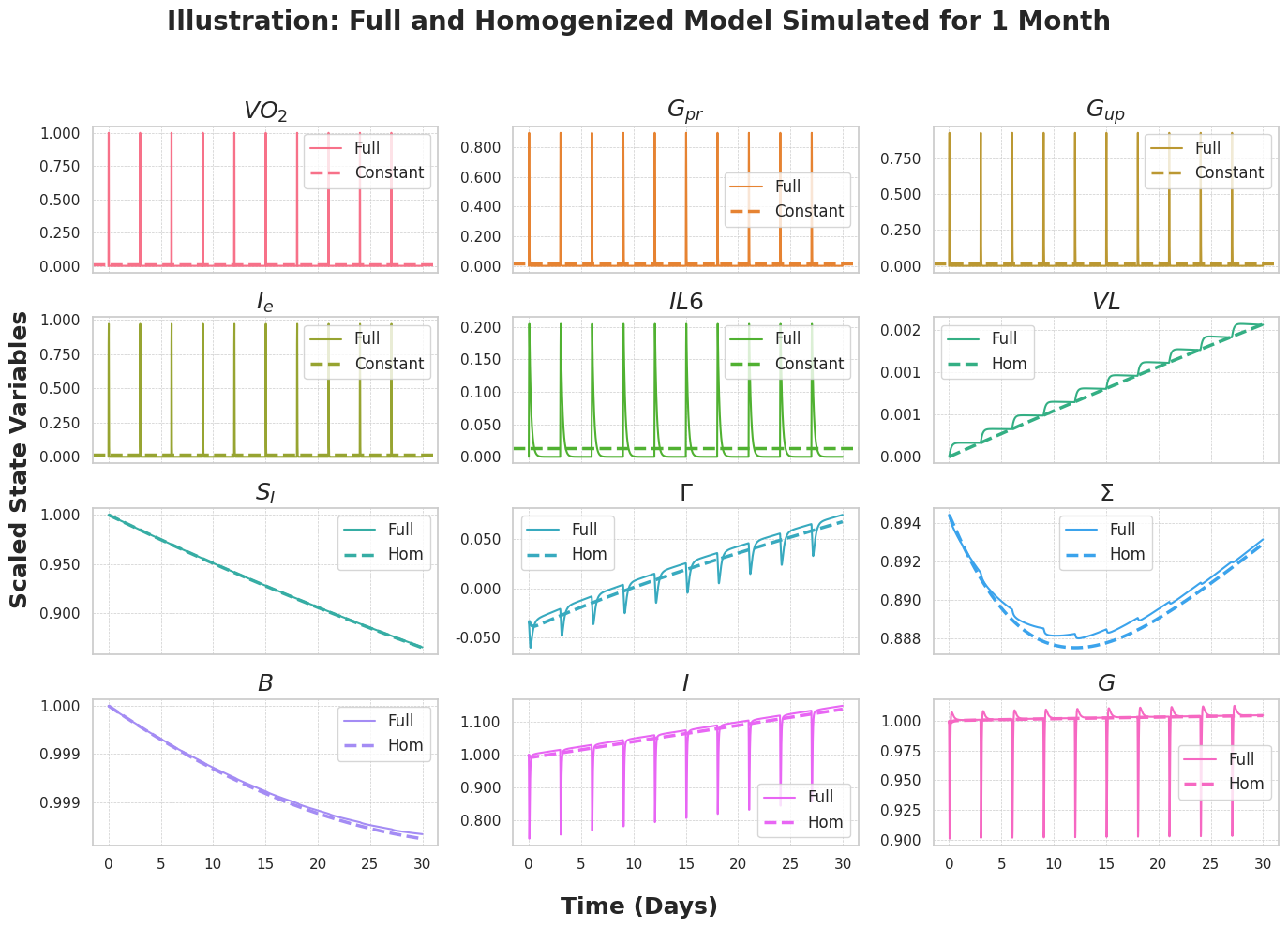
Figure 2. Illustration of the numerical solution of the full system (solid lines) and the homogenized system (dashed lines) for all 12 state variables for one month.

This figure illustrates how the short-term oscillations due to physical activity are smoothed in the homogenized system. All the parameters are chosen as outlined in Appendix 8.2.

To examine the long-term behavior of both the full and homogenized systems, we focus on the solutions at basal times, referring to the moments of the start of physical activity, i.e., at $t_{k}\mathrel{\mathrel{\mathop{:}}=}k\nu$ for $k=1,\dots,n$ with $t_{n}=t_{\mathrm{end}}$. Figure 3 presents the solutions of the full and homogenized systems at these basal times over a five-year period, again with the parameters from Appendix 8.2.

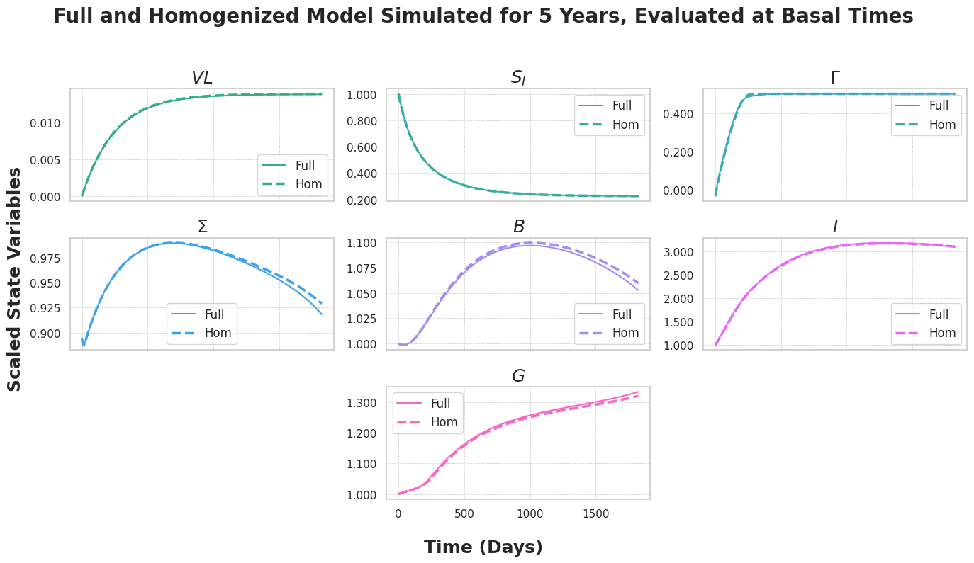
Figure 3. Solution at basal times (moments of the start of physical activity) of the full system (solid lines) and the homogenized system (dashed) for five years.

This figure demonstrates that the two systems exhibit very similar behavior over time.

4.2. Approximation error

To assess the numerical error made by homogenizing the system in practice, we vary six parameters and three initial conditions, as outlined in Table 1.

Table 1. Parameters (top) and initial conditions (bottom) that are varied for the numerical evaluation of the approximation error, resulting in $3^{9}=19\,683$ simulations.

Parameter	Values
$\nu$	2,4,6
$\delta$	30/1440,45/1440,60/1440
$\xi$	20,40,60
$\theta_{S_{\mathrm{I}}}$	0.18,0.28,0.38
$\tau_{S_{\mathrm{I}}}$	90,210,330
$\omega$	50,90,130
$B_{0}$	800,1000,1200
$I_{0}$	5,10,15
$G_{0}$	70,90,110

We denote each parameter configuration by $\Theta_{i}$, where $i=1,\dots,19\,683$, and solve the full and the homogenized systems with all possible $19\,683$ combinations for $T=1820$ days (corresponding to 5 years). The solutions are evaluated every 10 minutes, i.e., at $t_{m}\mathrel{\mathrel{\mathop{:}}=}m/144$, where $m=1,\dots,1820\cdot 144$. In correspondence with the approximation error defined in Subsection 3.3, we define the maximal deviation over 5 years between the full and the homogenized system for every simulation $i$ as

$$E_{i}\mathrel{\mathrel{\mathop{:}}=}\max_{m=1,\dots,1820\cdot 144}|\mathbf{y}(t_{m},u,\Theta_{i})-\widehat{\mathbf{y}}(t_{m},\Theta_{i})|\in\mathbb{R}^{12}.$$

A box plot summarizing the distribution of $E_{i}$ across the $19\,683$ simulations is given in Figure 4.

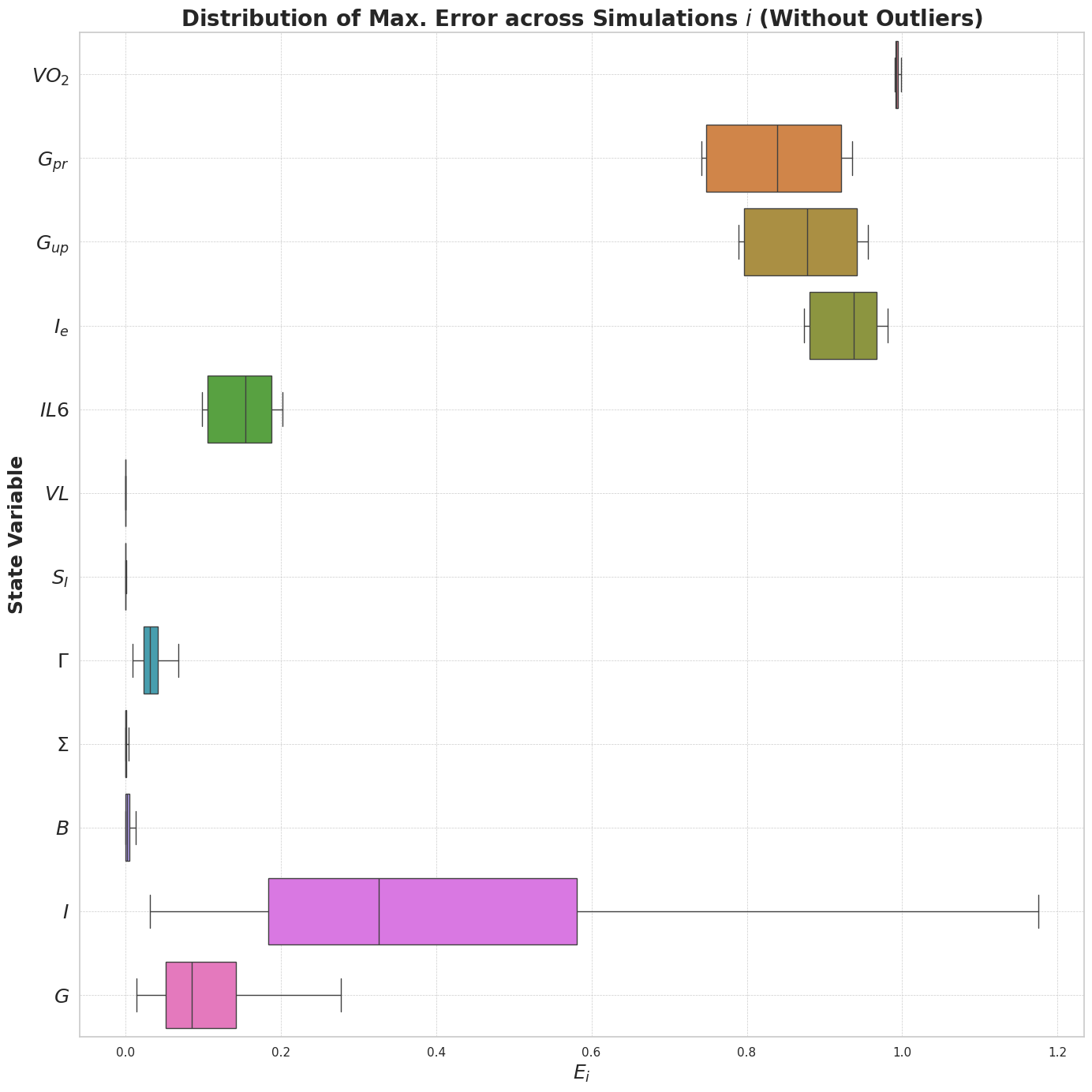
Figure 4. Box plot showing the distribution of the maximal deviation $E_{i}$ between the full and the homogenized system across $19\,683$ simulations.

Note that the maximal deviation of the state variables is made for the short-term variables $[V\!O_{2},G_{\mathrm{pr}},G_{\mathrm{up}},I_{\mathrm{e}},I\!L6]^{T}$, visualized in the upper part of Figure 4. By construction, this error is almost 1 as it accounts for the oscillations of the full system. However, it does not increase over time, unlike what would occur with a different norm. These findings underline the proof of Subsection 3.3, stating that the error is bounded by a constant depending on $t_{\mathrm{end}}$.

4.3. Point error after 5 years

The maximal deviation discussed above is a pessimistic estimate, as it is primarily influenced by the error in the oscillations At basal times, i.e., at $t_{k}$ for $k=1,\dots,n$, the error is significantly smaller. Here we illustrate the error after the simulating the system for 5 years, i.e., at $t_{\mathrm{end}}=n\nu$. Specifically, we define the point error at 5 years as

$$E_{i}^{5y}\mathrel{\mathrel{\mathop{:}}=}|\mathbf{y_{2}}(t_{\mathrm{end}},\mathbf{y_{1}},\Theta_{i})-\widehat{\mathbf{y_{2}}}(t_{\mathrm{end}},\mathbf{\mu},\Theta_{i})|\in\mathbb{R}^{7}.$$

A box plot summarizing the distribution of $E_{i}^{5y}$ across the $19\,683$ simulations is given in Figure 5.

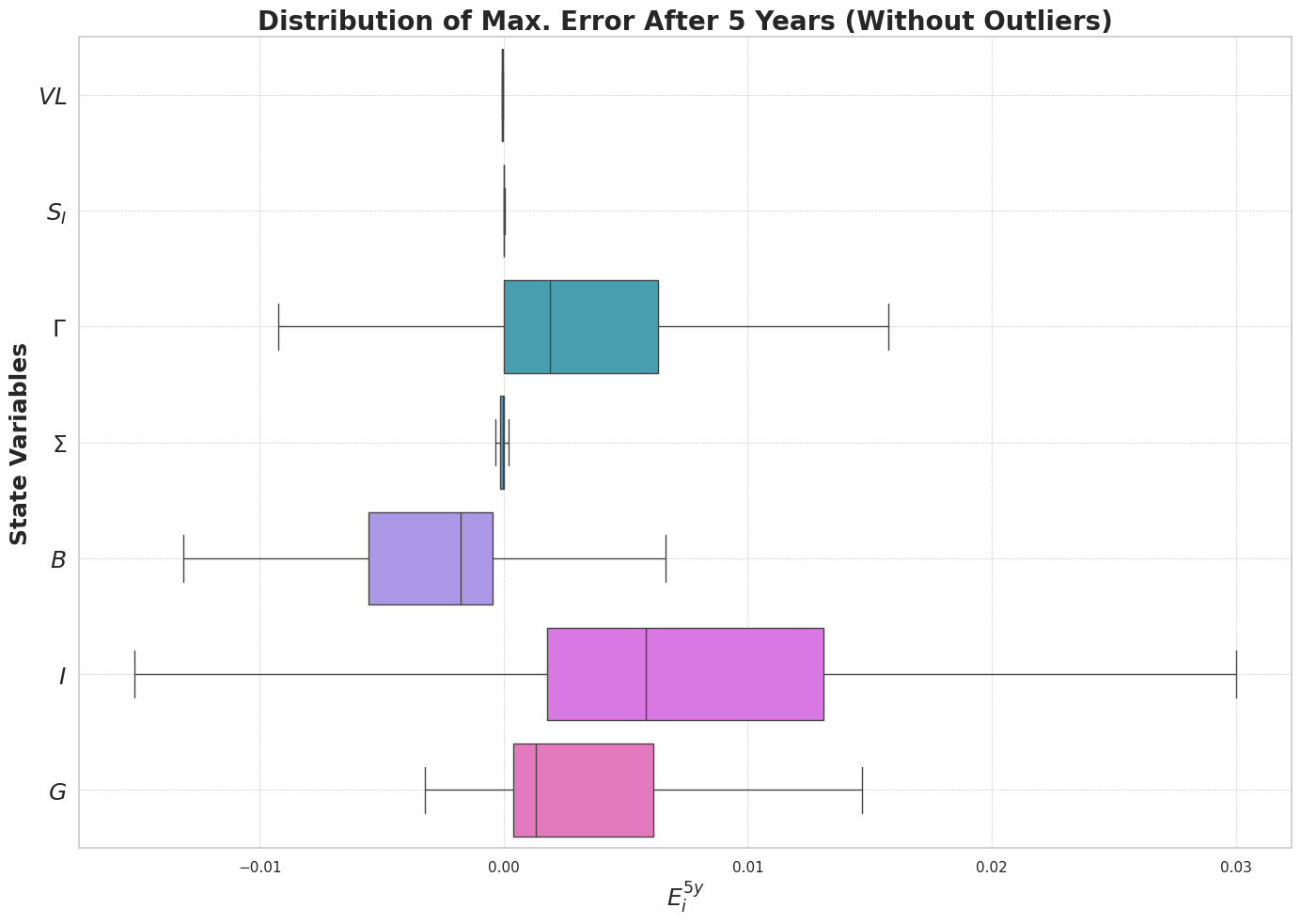
Figure 5. Box plot showing the distribution of the maximal deviation $E_{i}^{5y}$ between the full and the homogenized system across $i$ simulations after 5 years.

Note that, in comparison to Figure 4, these errors are much smaller. These results are presented with the scaling chosen in Appendix 8.1, a different scaling would yield a different comparison between the state variables. In conclusion, the final error in glucose $G$ is reasonably small and the homogenized system closely resembles the full system, achieving results $\lambda_{t}$ times faster.

5. Discussion

In this work, we have developed and analyzed a periodically homogenized version of a two-scale model capturing the long-term effects of physical activity on blood glucose regulation. The periodic nature of the physical activity control allowed us to homogenize the model analytically. This reduced model retains the essential dynamics of the original system while significantly reducing its computational cost. By treating the problem as a perturbation of the right-hand side, we have proven that the error introduced by the homogenization remains bounded over time. These theoretical results were underlined with a simulation study where we have varied nine key parameters of the model and assessed the maximal error between the two systems.

The full model, as described in Section 2 and previously published by De Paola et al. [10, 9], provides a detailed mechanistic explanation of how exercise affects glucose regulation over years. In this work, we have built upon these contributions by introducing a computationally fast version of the model, applicable under the assumption that physical activity follows a consistent periodic pattern over the years. In addition, we have introduced a mathematical perspective to the original formulation by scaling the equations for stability and by proving existence and uniqueness of both the full and the homogenized systems. This complements the previous focus on physiological mechanisms.

The homogenized model reduces the simulation time by more than a factor 1000, reflecting the shift from simulating processes on a minute scale to capturing the macro-dynamics on a day scale. This considerable reduction paves the way for the use of the homogenized model in the field of medical decision support. Personalized physical activity plans, along with the uncertainty around their impact, can be evaluated based on multiple runs of the model, for example in a Bayesian framework.

Moving forward, we are focusing on integrating the homogenized model into a causal learning framework. This will allow us to assess the effectiveness of hypothetical physical activity plans in slowing down or even preventing progression to type 2 diabetes in simulated at-risk individuals. However, the applicability of this model extends beyond diabetes prevention. From a theoretical point of view, the homogenized model offers a robust formulation of a physiological process, characterized by seven state variables and a control-like structure that introduces stiffness. We believe this model can be a valuable tool for researchers seeking to apply theoretical results to a well-studied, physiologically relevant system of ordinary differential equations.

6. Acknowledgment

This work was supported by the European Union and by the Swiss State Secretariat for Education, Research and Innovation (SERI) through project PRAESIIDIUM ”Physics informed machine learning-based prediction and reversion of impaired fasting glucose management” under Grant 101095672. Views and opinions expressed are however those of the authors only and do not necessarily reflect those of the European Union and SERI. The European Union and SERI cannot be held responsible for them.

Pierluigi Francesco De Paola is a PhD student enrolled in the National PhD Program in Autonomous Systems (DAUSY), coordinated by Politecnico of Bari, Bari, Italy.

Marta Lenatti is a PhD student enrolled in the National PhD in Artificial Intelligence, XXXVIII cycle, course on Health and life sciences, organized by Università Campus Bio-Medico di Roma.

The authors thank Fabrizio Dabbene, Alessandro Borri and Pasquale Palumbo for their valuable discussions about the full model.

7. Code availability

The code will be made publicly available upon acceptance of this manuscript.

8. Appendix

8.1. Scaling of the model

We adopt the following notation: state variables are represented by capital letters, using either Greek or Latin characters. Parameters are consistently denoted by lowercase Greek letters and may include subscripts. Functions are denoted by lowercase Latin letters, and also may include subscripts.

8.1.1. Scaling of the short-term equations

In this subsection, we rescale the original system [10, 9] based on the magnitude of the state variables and introduce a unified timescale. The short-term equations on a minute timescale read

$$\frac{\mathrm{d}}{\mathrm{d}t}V\!O_{2} =\theta u(t)-\theta V\!O_{2},$$

$$\frac{\mathrm{d}}{\mathrm{d}t}G_{\mathrm{pr}} =\alpha_{1}V\!O_{2}-\alpha_{2}G_{\mathrm{pr}},$$

$$\frac{\mathrm{d}}{\mathrm{d}t}G_{\mathrm{up}} =\alpha_{3}V\!O_{2}-\alpha_{4}G_{\mathrm{up}},$$

$$\frac{\mathrm{d}}{\mathrm{d}t}I_{\mathrm{e}} =\alpha_{5}V\!O_{2}-\alpha_{6}I_{\mathrm{e}},$$

$$\frac{\mathrm{d}}{\mathrm{d}t}I\!L6 =\kappa_{\mathrm{SR}}V\!O_{2}-\kappa_{\mathrm{IL6}}I\!L6,$$

$$\frac{\mathrm{d}}{\mathrm{d}t}V\!L =I\!L6-\kappa_{\mathrm{s}}V\!L,$$

with the initial conditions being $0$ for all the equations. The control $u(t)$ is introduced as

$$u(t)=\begin{cases}\xi&\text{for }0\leq t\leq\text{duration (min)},\\ 0&\text{for }\text{duration (min)}<t<\text{period length (min)},\end{cases}$$

where $\xi$ is the physical activity intensity. The term period length refers to the length from the start of one physical activity session until the start of the next session. Note that the state variable $V\!L$ is included in these equations because it was originally parameterized in minutes.

The original units of the state variables, along with their description, are given in Table 2.

Table 2. Short description and units of the short-term state variables in their unscaled form.

Variable	Description	Unit
$V\!O_{2}$	Oxygen consumption during exercise	given in %
$G_{\mathrm{pr}}$	Incremental hepatic glucose production	mg/(kg min)
$G_{\mathrm{up}}$	Increased glucose uptake by working tissues	mg/(kg min)
$I_{\mathrm{e}}$	Incremental insulin removal	$\mu$U/ml
$I\!L6$	Concentration of IL-6 in the muscle	pg/ml
$V\!L$	Integral effect of IL-6 released during exercise	(pg/ml) min

To solve these ODEs simultaneously with the long-term equations defined at a daily timescale, we first convert the short-term equations to days. Additionally, we scale the state variables to be dimensionless. Following standard procedures for the scaling of ODEs [13], we introduce

$$\overline{t}\mathrel{\mathrel{\mathop{:}}=}\frac{t}{\lambda_{t}}\;\text{and}\;\overline{\Omega}\mathrel{\mathrel{\mathop{:}}=}\frac{\Omega}{\lambda_{\Omega}},\;\Omega\in\{t,V\!O_{2},G_{\mathrm{pr}},G_{\mathrm{up}},I_{\mathrm{e}},I\!L6,V\!L\}.$$

Substituting this into both sides of the unscaled system and then rearranging yields

$$\frac{\mathrm{d}}{\mathrm{d}\overline{t}}\overline{V\!O_{2}} =\lambda_{t}\bigg{(}\frac{\theta}{\lambda_{V\!O_{2}}}u(\lambda_{t}\overline{t})-\theta\overline{V\!O_{2}}\bigg{)},$$

$$\frac{\mathrm{d}}{\mathrm{d}\overline{t}}\overline{G_{\mathrm{pr}}} =\lambda_{t}\bigg{(}\frac{\alpha_{1}\lambda_{V\!O_{2}}}{\lambda_{G_{\mathrm{pr}}}}\overline{V\!O_{2}}-\alpha_{2}\overline{G_{\mathrm{pr}}}\bigg{)},$$

$$\frac{\mathrm{d}}{\mathrm{d}\overline{t}}\overline{G_{\mathrm{up}}} =\lambda_{t}\bigg{(}\frac{\alpha_{3}\lambda_{V\!O_{2}}}{\lambda_{G_{\mathrm{up}}}}\overline{V\!O_{2}}-\alpha_{4}\overline{G_{\mathrm{up}}}\bigg{)},$$

$$\frac{\mathrm{d}}{\mathrm{d}\overline{t}}\overline{I_{\mathrm{e}}} =\lambda_{t}\bigg{(}\frac{\alpha_{5}\lambda_{V\!O_{2}}}{\lambda_{I_{\mathrm{e}}}}\overline{V\!O_{2}}-\alpha_{6}\overline{I_{\mathrm{e}}}\bigg{)},$$

$$\frac{\mathrm{d}}{\mathrm{d}\overline{t}}\overline{I\!L6} =\lambda_{t}\bigg{(}\frac{\kappa_{\mathrm{SR}}\lambda_{V\!O_{2}}}{\lambda_{I\!L6}}\overline{V\!O_{2}}-\kappa_{\mathrm{IL6}}\overline{I\!L6}\bigg{)},$$

$$\frac{\mathrm{d}}{\mathrm{d}\overline{t}}\overline{V\!L} =\lambda_{t}\bigg{(}\frac{\lambda_{I\!L6}}{\lambda_{V\!L}}\overline{I\!L6}-\kappa_{\mathrm{s}}\overline{V\!L}\bigg{)}.$$

The initial conditions are $0$ for all equations, hence no scaling is necessary. We now select the scaling constants as specified in Appendix 8.2. Note that the choice of $\lambda_{t}$ transforms the time from minutes to days. All the other constants are chosen to make the state variables unitless and to scale the system to take values in the interval $[0,1]$. We conclude the scaling of the short-term state variables by noting that to include these variables in the long-term equations, they need to be rescaled to their original units and, subsequently, the state variables containing minutes as units need to be transformed to days as follows

$$G_{\mathrm{pr}}^{\textrm{day}}\mathrel{\mathrel{\mathop{:}}=}\lambda_{t}G_{\mathrm{pr}},\;G_{\mathrm{up}}^{\textrm{day}}\mathrel{\mathrel{\mathop{:}}=}\lambda_{t}G_{\mathrm{up}},\;V\!L^{\textrm{day}}\mathrel{\mathrel{\mathop{:}}=}\frac{V\!L}{\lambda_{t}}.$$

8.1.2. Auxiliary functions for the long-term equations

Before presenting the long-term equations, we provide a concise overview of a set of auxiliary functions originally introduced in the appendix of the publication by Ha et al. [11].

We first define the two functions $q_{h}$ and $q_{e}$ as follows:

$$q_{h}(x;\pi_{1},\pi_{2}) \mathrel{\mathrel{\mathop{:}}=}\frac{x^{\pi_{2}}}{x^{\pi_{2}}+\pi_{1}^{\pi_{2}}},\;\text{for}\;\pi_{1}\in\mathbb{R}^{+},\;\pi_{2}\in 2\mathbb{N}^{+},$$

$$q_{e}(x;\pi_{1},\pi_{2},\pi_{3},\pi_{4}) \mathrel{\mathrel{\mathop{:}}=}\frac{\pi_{1}}{1+\pi_{4}\exp\big{(}-\frac{x-\pi_{2}}{\pi_{3}}\big{)}}\;\text{for}\;\pi_{1},\pi_{2},\pi_{3},\pi_{4}\in\mathbb{R}^{+},$$

where $x\in\mathbb{R}$. Under the listed constraints on the constants, both functions are Lipschitz-continuous and bounded in $x$. With these functions at hand, we define the following auxiliary functions, following the notation of the original publications wherever possible. A list of all the parameters introduced here can be found in Appendix 8.2. The first set of functions requires the Hill-type function $q_{h}$:

$$m(G) =q_{h}(G;\alpha_{\mathrm{M}},2),$$

$$r(\Gamma,\Sigma,G) =\Sigma q_{h}\big{(}m(G)+\Gamma;\alpha_{\mathrm{ISR}},2\big{)},$$

$$p(V\!L,\Gamma,\Sigma,G) =\phi_{\mathrm{max}}q_{h}\big{(}r(\Gamma,\Sigma,G);\alpha_{\mathrm{P}},4\big{)}\big{(}1+\zeta_{1}q_{h}(V\!L;\kappa_{\mathrm{n}},2)\big{)},$$

$$a(V\!L,G) =\Big{(}\alpha_{\mathrm{max}}q_{h}\big{(}m(G);\alpha_{\mathrm{A}},6\big{)}+\alpha_{\mathrm{B}}\Big{)}\Big{(}1-\zeta_{2}q_{h}(V\!L;\kappa_{\mathrm{n}},2)\Big{)}.$$

It is clear that all of these functions are Lipschitz-continuous with respect to all of their arguments. Furthermore, it can easily be verified that the functions $m$, $p$ and $a$ are bounded. The function $r$ is only bounded if $\Sigma$ is bounded.

The second set requires the function $q_{e}$:

$$g_{\infty}(G) =q_{e}(G;\gamma_{\mathrm{max}},\gamma_{\mathrm{S}},\gamma_{\mathrm{n}},1)-\gamma_{\theta},$$

$$s_{\mathrm{ISR\infty}}(\Gamma,\Sigma,G) =q_{e}\big{(}r(\Gamma,\Sigma,G-\kappa_{\sigma\mathrm{s}});\sigma_{\mathrm{ISRmax}},\sigma_{\mathrm{ISRs}},\sigma_{\mathrm{ISRn}},\sigma_{\mathrm{ISRk}}\big{)},$$

$$s_{\mathrm{M\infty}}(G) =1-q_{e}\big{(}m(G-\kappa_{\sigma\mathrm{s}});\sigma_{\mathrm{Mmax}},\sigma_{\mathrm{Ms}},\sigma_{\mathrm{Mn}},\sigma_{\mathrm{Mk}}\big{)},$$

$$s_{\infty}(\Gamma,\Sigma,G) =s_{\mathrm{ISR\infty}}(\Gamma,\Sigma,G)s_{\mathrm{M\infty}}(G)+\sigma_{\mathrm{B}}.$$

Again, it is clear that all of these functions are Lipschitz-continuous and bounded in all of their arguments, as long as all of the parameters are positive.

8.1.3. Scaling of the long-term equations

The long-term equations are written down in the original publication as follows:

$$\frac{\mathrm{d}}{\mathrm{d}t}S_{\mathrm{I}} =\bigg{(}\frac{\theta_{S_{\mathrm{I}}}-S_{\mathrm{I}}}{\tau_{S_{\mathrm{I}}}}\bigg{)}\bigg{(}1-\zeta_{3}\frac{V\!L^{\textrm{day}}}{k_{nS_{\mathrm{I}}}+V\!L^{\textrm{day}}}\bigg{)},$$

$$\frac{\mathrm{d}}{\mathrm{d}t}\Gamma =\frac{g_{\infty}(G)-\Gamma}{\tau_{\Gamma}},$$

$$\frac{\mathrm{d}}{\mathrm{d}t}\Sigma =\frac{s_{\infty}(\Gamma,\Sigma,G)-\Sigma}{\tau_{\Sigma}},$$

$$\frac{\mathrm{d}}{\mathrm{d}t}B =\frac{p(V\!L^{\textrm{day}},\Gamma,\Sigma,G)-a(V\!L^{\textrm{day}},G)}{\tau_{B}}B,$$

$$\frac{\mathrm{d}}{\mathrm{d}t}I =\frac{r(\Gamma,\Sigma,G)}{\upsilon}B-\kappa I-I_{\mathrm{e}},$$

$$\frac{\mathrm{d}}{\mathrm{d}t}G =\rho_{0}+\frac{\omega}{\upsilon_{g}}(G_{\mathrm{pr}}^{\textrm{day}}-G_{\mathrm{up}}^{\textrm{day}})-(\eta_{0}+S_{\mathrm{I}}I)G,$$

with initial conditions $S_{\mathrm{I}}(0)={S_{\mathrm{I}}}_{0}$, $\Gamma(0)=\Gamma_{0}$, $\Sigma(0)=\Sigma_{0}$, $B(0)=B_{0}$, $I(0)=I_{0}$ and $G(0)=G_{0}$. The five auxiliary functions $g_{\infty}$, $s_{\infty}$, $p$, $a$ and $r$ have been defined above. The original units of the introduced long-term state variables, along with their description, are given in Table 3.

Table 3. Short description and units of the long-term state variables in their unscaled form.

Variable	Description	Unit
$S_{\mathrm{I}}$	Insulin sensitivity	$\mu$U/($\mu$g day)
$\Gamma$	Shift of the glucose dependence	-
$\Sigma$	Insulin secretion capacity	$\mu$U/ ($\mu$g day)
$B$	Beta cell mass	mg
$I$	Serum insulin concentration	$\mu$U/ml
$G$	Plasma glucose concentration	mg/dl

Again, we introduce the following scaling of the state variables

$$\overline{\Omega}\mathrel{\mathrel{\mathop{:}}=}\frac{\Omega}{\lambda_{\Omega}},\;\Omega\in\{S_{\mathrm{I}},\Gamma,\Sigma,B,I,G\}.$$

The chosen scaling parameters, along with all the parameters introduced, are listed in Appendix 8.2. Note that $t$ does not require scaling since we want to solve the final system in days. For simplification, we introduce the following auxiliary functions:

(7) $$d_{\lambda}\big{(}\overline{V\!L}\big{)} \mathrel{\mathrel{\mathop{:}}=}\frac{1}{{\lambda_{S_{\mathrm{I}}}}}\Bigg{(}1-\zeta_{3}\bigg{(}\frac{(\lambda_{V\!L}/\lambda_{t})\overline{V\!L}}{\kappa_{\mathrm{n}S_{\mathrm{I}}}+(\lambda_{V\!L}/\lambda_{t})\overline{V\!L}}\bigg{)}\Bigg{)},$$

$$g_{\lambda}\big{(}\overline{G}\big{)} \mathrel{\mathrel{\mathop{:}}=}\frac{1}{\lambda_{\Gamma}}g_{\infty}\big{(}\lambda_{G}\overline{G}\big{)},$$

$$s_{\lambda}\big{(}\overline{\Gamma},\overline{\Sigma},\overline{G}\big{)} \mathrel{\mathrel{\mathop{:}}=}\frac{1}{\lambda_{\Sigma}}s_{\infty}\big{(}\lambda_{\Gamma}\overline{\Gamma},\lambda_{\Sigma}\overline{\Sigma},\lambda_{G}\overline{G}\big{)}$$

$$p_{\lambda}\big{(}\overline{V\!L},\overline{\Gamma},\overline{\Sigma},\overline{G}\big{)} \mathrel{\mathrel{\mathop{:}}=}p\big{(}(\lambda_{V\!L}/\lambda_{t})\overline{V\!L},\lambda_{\Gamma}\overline{\Gamma},\lambda_{\Sigma}\overline{\Sigma},\lambda_{G}\overline{G}\big{)},$$

$$a_{\lambda}\big{(}\overline{V\!L},\overline{G}\big{)} \mathrel{\mathrel{\mathop{:}}=}a\big{(}(\lambda_{V\!L}/\lambda_{t})\overline{V\!L},\lambda_{G}\overline{G}\big{)},$$

$$r_{\lambda}\big{(}\overline{\Gamma},\overline{\Sigma},\overline{G}\big{)} \mathrel{\mathrel{\mathop{:}}=}\frac{\lambda_{B}}{\lambda_{I}\upsilon}r\big{(}\lambda_{\Gamma}\overline{\Gamma},\lambda_{\Sigma}\overline{\Sigma},\lambda_{G}\overline{G}\big{)}.$$

We furthermore define the following constants:

$$\lambda_{I_{\mathrm{e}}I}\mathrel{\mathrel{\mathop{:}}=}\frac{\lambda_{I_{\mathrm{e}}}}{\lambda_{I}},\quad\rho_{\lambda}\mathrel{\mathrel{\mathop{:}}=}\frac{\rho_{0}}{\lambda_{G}},\quad\lambda_{tG}\mathrel{\mathrel{\mathop{:}}=}\frac{\lambda_{t}}{\lambda_{G}\upsilon_{g}},\quad\lambda_{S_{\mathrm{I}}I}\mathrel{\mathrel{\mathop{:}}=}\lambda_{S_{\mathrm{I}}}\lambda_{I}.$$

After substituting the scaling parameters and rewriting, we obtain the following system of ODEs:

$$\frac{\mathrm{d}}{\mathrm{d}t}\overline{S_{\mathrm{I}}} =d_{\lambda}\big{(}\overline{V\!L}\big{)}\bigg{(}\frac{\theta_{S_{\mathrm{I}}}-\lambda_{S_{\mathrm{I}}}\overline{S_{\mathrm{I}}}}{\tau_{S_{\mathrm{I}}}}\bigg{)},$$

$$\frac{\mathrm{d}}{\mathrm{d}t}\overline{\Gamma} =\frac{g_{\lambda}\big{(}\overline{G}\big{)}-\overline{\Gamma}}{\tau_{\Gamma}},$$

$$\frac{\mathrm{d}}{\mathrm{d}t}\overline{\Sigma} =\frac{s_{\lambda}\big{(}\overline{\Gamma},\overline{\Sigma},\overline{G}\big{)}-\overline{\Sigma}}{\tau_{\Sigma}},$$

$$\frac{\mathrm{d}}{\mathrm{d}t}\overline{B} =\frac{p_{\lambda}\big{(}\overline{V\!L},\overline{\Gamma},\overline{\Sigma},\overline{G}\big{)}-a_{\lambda}\big{(}\overline{V\!L},\overline{G}\big{)}}{\tau_{B}}\overline{B},$$

$$\frac{\mathrm{d}}{\mathrm{d}t}\overline{I} =r_{\lambda}\big{(}\overline{\Gamma},\overline{\Sigma},\overline{G}\big{)}\overline{B}-\kappa\overline{I}-\lambda_{I_{\mathrm{e}}I}\overline{I_{\mathrm{e}}},$$

$$\frac{\mathrm{d}}{\mathrm{d}t}\overline{G} =\rho_{\lambda}+\lambda_{tG}\omega\big{(}\lambda_{G_{\mathrm{pr}}}\overline{G_{\mathrm{pr}}}-\lambda_{G_{\mathrm{up}}}\overline{G_{\mathrm{up}}}\big{)}-(\eta_{0}+\lambda_{S_{\mathrm{I}}I}\overline{S_{\mathrm{I}}}\overline{I})\overline{G},$$

together with the initial conditions $S_{\mathrm{I}}(0)=1$, $\Gamma(0)=\Gamma_{0}/\gamma_{\textrm{max}}\mathrel{=\mathrel{\mathop{:}}}\Gamma_{0\lambda}$, $\Sigma(0)=\Sigma_{0}/\sigma_{\mathrm{ISRmax}}\mathrel{=\mathrel{\mathop{:}}}\Sigma_{0\lambda}$, $B(0)=1$, $I(0)=1$ and $G(0)=1$.

8.2. Parameters

A list of the parameters introduced in the short-term equations ($\mathbf{y_{1}}$) can be found in Table 4.

Table 4. Parameters related to the control $u(t)$ (top), the system of ODEs for $\mathbf{y_{1}}$ (middle) and the scaling of $\mathbf{y_{1}}$ (bottom). Standard values or the formula and the respective units are given in columns 2 and 3.

Parameter	Value or Formula	Unit
$\nu$	3	day
$\delta$	60/1440	day
$\xi$	50	%
$\theta$	0.8	1/min
$\alpha_{1}$	0.00158	mg/(kg min2)
$\alpha_{2}$	0.056	1/min
$\alpha_{3}$	0.00195	mg/(kg min2)
$\alpha_{4}$	0.0485	1/min
$\alpha_{5}$	0.00125	$\mu$U/(ml min)
$\alpha_{6}$	0.075	1/min
$\kappa_{\mathrm{SR}}$	0.045	pg/(ml min)
$\kappa_{\mathrm{IL6}}$	0.004	1/min
$\lambda_{t}$	$1440$	min/day
$\lambda_{V\!O_{2}}$	$\xi$	given in %
$\lambda_{G_{\mathrm{pr}}}$	$\lambda_{V\!O_{2}}\alpha_{1}/\alpha_{2}$	mg/(kg min)
$\lambda_{G_{\mathrm{up}}}$	$\lambda_{V\!O_{2}}\alpha_{3}/\alpha_{4}$	mg/(kg min)
$\lambda_{I_{\mathrm{e}}}$	$\lambda_{V\!O_{2}}\alpha_{5}/\alpha_{6}$	$\mu$U/ml
$\lambda_{I\!L6}$	$\lambda_{V\!O_{2}}\kappa_{\mathrm{SR}}/\kappa_{\mathrm{IL6}}$	pg/ml

The parameters related to the state variable $V\!L$ are reported below together with the long-term state variables. The physical activity parameters $\nu$ and $\delta$ need to be chosen to allow for a maximum of 400 minutes of exercise per week, the intensity parameter $\xi$ needs to lay within $[0,92]\%$.

A list of the parameters introduced for the auxiliary functions can be found in Table 5.

Table 5. Parameters used for the auxiliary functions building upon $q_{h}$ (top) and the auxiliary functions building upon $q_{e}$ (bottom). Standard values or the formula and the respective units are given in columns 2 and 3.

Parameter	Value or Formula	Unit
$\alpha_{\mathrm{M}}$	150	mg/dl
$\alpha_{\mathrm{ISR}}$	1.2	-
$\phi_{\mathrm{max}}$	4.55	1/day
$\alpha_{\mathrm{P}}$	41.77	$\mu$U/($\mu$g day)
$\zeta_{1}$	$10^{-4}$	-
$\kappa_{\mathrm{n}}$	$10^{6}/\lambda_{t}$	(pg/ml) day
$\alpha_{\mathrm{max}}$	9	1/day
$\alpha_{\mathrm{A}}$	0.44	-
$\alpha_{\mathrm{B}}$	0.8	1/day
$\zeta_{2}$	$10^{-4}$	-
$\gamma_{\mathrm{max}}$	0.2	-
$\gamma_{\mathrm{S}}$	99.9	-
$\gamma_{\mathrm{n}}$	1	-
$\gamma_{\theta}$	0.1	-
$\kappa_{\sigma\mathrm{s}}$	75	mg/dl
$\sigma_{\mathrm{ISRmax}}$	600	$\mu$U/($\mu$g day)
$\sigma_{\mathrm{ISRs}}$	0.1	-
$\sigma_{\mathrm{ISRn}}$	0.1	-
$\sigma_{\mathrm{ISRk}}$	1	-
$\sigma_{\mathrm{Mmax}}$	1	-
$\sigma_{\mathrm{Ms}}$	0.2	-
$\sigma_{\mathrm{Mn}}$	0.02	-
$\sigma_{\mathrm{Mk}}$	0.2	-
$\sigma_{\mathrm{B}}$	3	$\mu$U/($\mu$g day)

All of these parameters are constrained to be positive.

A list of the parameters introduced for the long-term equations can be found in Table 6.

Table 6. Parameters related to the system of ODEs for $\mathbf{y_{2}}$ (top), the scaling of $\mathbf{y_{2}}$ (middle) and the initial conditions for $\mathbf{y_{2}}$ (bottom). Standard values or the formula and the respective units are given in columns 2 and 3.

Parameter	Value or Formula	Unit
$\kappa_{\mathrm{s}}$	$-\log(0.8)/(8\times 7\times 1440)$	1/min
$\theta_{S_{\mathrm{I}}}$	0.18	$\mu$U/($\mu$g day)
$\tau_{S_{\mathrm{I}}}$	150	day
$\zeta_{3}$	1.4	-
$k_{nS_{\mathrm{I}}}$	$5\times 10^{6}/\lambda_{t}$	(pg/ml) day
$\tau_{\Gamma}$	2.14	day
$\tau_{\Sigma}$	249.9	day
$\tau_{B}$	8570	day
$\upsilon$	5	litre
$\kappa$	700	1/day
$\rho_{0}$	864	mg/(dl day)
$\omega$	70	kg
$\upsilon_{g}$	117	dl
$\eta_{0}$	1.44	1/day
$\lambda_{V\!L}/\lambda_{t}$	$(\lambda_{I\!L6}/\kappa_{\mathrm{s}})/\lambda_{t}$	(pg/ml)day
$\lambda_{S_{\mathrm{I}}}$	${S_{\mathrm{I}}}_{0}$	$\mu$U/($\mu$g day)
$\lambda_{\Gamma}$	$\gamma_{\mathrm{max}}$	-
$\lambda_{\Sigma}$	$\sigma_{\mathrm{ISRmax}}$	$\mu$U/($\mu$g day)
$\lambda_{B}$	$B_{0}$	mg
$\lambda_{I}$	$I_{0}$	$\mu$U/ml
$\lambda_{G}$	$G_{0}$	mg/dl
$\lambda_{I_{\mathrm{e}}I}$	$\lambda_{I_{\mathrm{e}}}/\lambda_{I}$	-
$\rho_{\lambda}$	$\rho_{0}/\lambda_{G}$	1/day
$\lambda_{tG}$	$\lambda_{t}/(\lambda_{G}\upsilon_{g})$	min/(mg day)
$\lambda_{S_{\mathrm{I}}I}$	$\lambda_{S_{\mathrm{I}}}\lambda_{I}$	$\mu\text{U}^{2}$/($\mu$g day ml)
$V\!L_{0}$	0	(pg/ml) min
${S_{\mathrm{I}}}_{0}$	0.8	$\mu$U/($\mu$g day)
$\Gamma_{0}$	-0.00666	-
$\Sigma_{0}$	536.67	$\mu$U/ ($\mu$g day)
$B_{0}$	1000.423	mg
$I_{0}$	9.025	$\mu$U/ml
$G_{0}$	99.7604	mg/dl
$\Gamma_{0\lambda}$	$\Gamma_{0}/\lambda_{\Gamma}$	-
$\Sigma_{0\lambda}$	$\Sigma_{0}/\lambda_{\Sigma}$	-

The units of some parameters in Table 6 are scaled with $\lambda_{t}$ in order to be in days. Based on expert opinion, the initial conditions should be in the following intervals: ${S_{\mathrm{I}}}_{0}\in[0,0.8]$, $\Gamma_{0}\in[-0.1,0.1]$, $\Sigma_{0}\in[3,600]$, $B_{0}\in[0,9000]$, $I_{0}\in[0,100]$, $G_{0}\in[0,600]$.

8.3. Analytical solution of the model for the first period

We calculate the analytical solution $V\!O_{2}$ from System (3) first in the interval $[0,\delta]$, where the control $u(t)=1$, then use the value at $\delta$ as initial condition to solve the ODEs analytically in the interval $(\delta,\nu)$, where $u(t)=0$:

Lemma 8.1.

The solution to $V\!O_{2}^{\prime}(t)=\lambda_{t}\theta\big{(}1-V\!O_{2}(t)\big{)}$ for $0<t\leq\delta$ with initial condition $V\!O_{2}(0)=0$ is given by

$$V\!O_{2}(t)=1-\exp(-\lambda_{t}\theta t).$$

Inserting $\delta$ yields $V\!O_{2}(\delta)=1-\exp(-\lambda_{t}\theta\delta)$, which is the initial condition for the next interval:

Lemma 8.2.

The solution to $V\!O_{2}^{\prime}(t)=-\lambda_{t}\theta V\!O_{2}(t)$ for $\delta<t<\nu$ with initial condition $V\!O_{2}(\delta)=1-\exp(-\lambda_{t}\theta\delta)$ is given by

$$V\!O_{2}(t)=\big{(}\exp(\lambda_{t}\theta\delta)-1\big{)}\exp(-\lambda_{t}\theta t).$$

Calculating the analytical solution for the other four state variables from System (3) ($G_{\mathrm{pr}}$, $G_{\mathrm{up}}$, $I_{\mathrm{e}}$, $I\!L6$) follows the same steps, additionally using the analytical solution of $V\!O_{2}$. For the sake of simplicity, we just illustrate it for $G_{\mathrm{pr}}$:

Lemma 8.3.

The solution to $G_{\mathrm{pr}}^{\prime}(t)=\lambda_{t}\alpha_{2}\big{(}1-\exp(-\lambda_{t}\theta t)-G_{\mathrm{pr}}(t)\big{)}$ for $0<t\leq\delta$ with initial condition $G_{\mathrm{pr}}(0)=0$ is given by

$$G_{\mathrm{pr}}(t)=1+\frac{\alpha_{2}}{\theta-\alpha_{2}}\exp(-\lambda_{t}\theta t)-\frac{\theta}{\theta-\alpha_{2}}\exp(-\lambda_{t}\alpha_{2}t).$$

Inserting $\delta$ yields the initial condition for the next interval:

Lemma 8.4.

The solution to

$$G_{\mathrm{pr}}^{\prime}(t)=\lambda_{t}\alpha_{2}\Big{(}\big{(}\exp(\lambda_{t}\theta\delta)-1\big{)}\exp(-\lambda_{t}\theta t)-G_{\mathrm{pr}}(t)\Big{)}$$

for $\delta<t<\nu$ with initial condition

$$G_{\mathrm{pr}}(\delta)=1+\frac{\alpha_{2}}{\theta-\alpha_{2}}\exp(-\lambda_{t}\theta\delta)-\frac{\theta}{\theta-\alpha_{2}}\exp(-\lambda_{t}\alpha_{2}\delta)$$

is given by

$$G_{\mathrm{pr}}(t)= \frac{\theta}{\theta-\alpha_{2}}\big{(}\exp(\lambda_{t}\alpha_{2}\delta)-1\big{)}\exp(-\lambda_{t}\alpha_{2}t)$$

$$-\frac{\alpha_{2}}{\theta-\alpha_{2}}\big{(}\exp(\lambda_{t}\theta\delta)-1\big{)}\exp(-\lambda_{t}\theta t).$$

8.4. Homogenization for the first period

To calculate the average $\mu_{V\!O_{2}}$ of $V\!O_{2}(t)$ in the interval $[0,\nu)$, we start with

$$\int_{0}^{\delta}V\!O_{2}(t)\,\mathrm{d}t =\int_{0}^{\delta}1-\exp(-\lambda_{t}\theta t)\,\mathrm{d}t=\delta-\frac{1}{\lambda_{t}\theta}\big{(}1-\exp(-\lambda_{t}\theta\delta)\big{)},$$

$$\int_{\delta}^{\nu}V\!O_{2}(t)\,\mathrm{d}t =\frac{1}{\lambda_{t}\theta}\big{(}\exp(\lambda_{t}\theta\delta)-1\big{)}\Big{(}\exp(-\lambda_{t}\theta\delta)-\exp(-\lambda_{t}\theta\nu)\Big{)}$$

$$=\frac{1}{\lambda_{t}\theta}\Big{(}1-\exp(-\lambda_{t}\theta\delta)+\exp(-\lambda_{t}\theta\nu)\big{(}1-\exp(\lambda_{t}\theta\delta)\big{)}\Big{)}.$$

Combining these identities yields

$$\mu_{V\!O_{2}} =\frac{1}{\nu}\int_{0}^{\nu}V\!O_{2}(t)\,\mathrm{d}t=\frac{1}{\nu}\bigg{(}\int_{0}^{\delta}V\!O_{2}(t)\,\mathrm{d}t+\int_{\delta}^{\nu}V\!O_{2}(t)\,\mathrm{d}t\bigg{)}$$

$$=\frac{1}{\nu}\bigg{(}\delta+\frac{1}{\lambda_{t}\theta}\Big{(}\exp(-\lambda_{t}\theta\nu)\big{(}1-\exp(\lambda_{t}\theta\delta)\big{)}\Big{)}\bigg{)}.$$

Note that the result is approximately equal to $\delta/\nu$, which is the average value of $u(t)$.
For $G_{\mathrm{pr}}$, it holds that

$$\int_{0}^{\delta}G_{\mathrm{pr}}(t)\,\mathrm{d}t=\delta -\frac{\theta}{\lambda_{t}\alpha_{2}(\theta-\alpha_{2})}\big{(}1-\exp(-\lambda_{t}\alpha_{2}\delta)\big{)}$$

$$+\frac{\alpha_{2}}{\lambda_{t}\theta(\theta-\alpha_{2})}\big{(}1-\exp(-\lambda_{t}\theta\delta)\big{)},$$

and

$$\int_{\delta}^{\nu}G_{\mathrm{pr}}(t)\,\mathrm{d}t= \frac{\theta}{\lambda_{t}\alpha_{2}(\theta-\alpha_{2})}\Big{(} 1-\exp(-\lambda_{t}\alpha_{2}\delta)$$

$$+\exp(-\lambda_{t}\alpha_{2}\nu)\big{(}1-\exp(\lambda_{t}\alpha_{2}\delta)\big{)}\Big{)}$$

$$-\frac{\alpha_{2}}{\lambda_{t}\theta(\theta-\alpha_{2})}\Big{(} 1-\exp(-\lambda_{t}\theta\delta)$$

$$+\exp(-\lambda_{t}\theta\nu)\big{(}1-\exp(\lambda_{t}\theta\delta)\big{)}\Big{)}.$$

And hence,

$$\mu_{G_{\mathrm{pr}}} =\frac{1}{\nu}\bigg{(} \int_{0}^{\delta}G_{\mathrm{pr}}(t)\,\mathrm{d}t+\int_{\delta}^{\nu}G_{\mathrm{pr}}(t)\,\mathrm{d}t\bigg{)}$$

$$=\frac{1}{\nu}\bigg{(} \delta+\frac{\theta}{\lambda_{t}\alpha_{2}(\theta-\alpha_{2})}\Big{(}\exp(-\lambda_{t}\alpha_{2}\nu)\big{(}1-\exp(\lambda_{t}\alpha_{2}\delta)\big{)}\Big{)}$$

$$-\frac{\alpha_{2}}{\lambda_{t}\theta(\theta-\alpha_{2})}\Big{(}\exp(-\lambda_{t}\theta\nu)\big{(}1-\exp(\lambda_{t}\theta\delta)\big{)}\Big{)}\bigg{)}.$$

The mean values for the state variables $G_{\mathrm{up}}$, $I_{\mathrm{e}}$ and $I\!L6$ are calculated analogously to $G_{\mathrm{pr}}$.

References

• [1] G. Allaire, A Brief Introduction to Homogenization and Miscellaneous Applications, ESAIM: Proceedings, 37 (2012), pp. 1–49.
• [2] N. Bakhvalov and G. Panasenko, Homogenisation: Averaging Processes in Periodic Media, vol. 36 of Mathematics and its Applications, Springer Netherlands, Dordrecht, 1989.
• [3] R. Bergman, Minimal Model: Perspective from 2005, Hormone Research in Paediatrics, 64 (2005), pp. 8–15.
• [4] R. Bergman, L. Phillips, and C. Cobelli, Physiologic Evaluation of Factors Controlling Glucose Tolerance in Man: Measurement of Insulin Sensitivity and Beta-Cell Glucose Sensitivity from the Response to Intravenous Glucose., Journal of Clinical Investigation, 68 (1981), pp. 1456–1467.
• [5] F. Bull, S. Al-Ansari, S. Biddle, K. Borodulin, M. P. Buman, G. Cardon, C. Carty, J. Chaput, S. Chastin, R. Chou, P. Dempsey, L. DiPietro, U. Ekelund, J. Firth, C. Friedenreich, L. Garcia, M. Gichu, R. Jago, P. Katzmarzyk, E. Lambert, M. Leitzmann, K. Milton, F. B. Ortega, C. Ranasinghe, E. Stamatakis, A. Tiedemann, R. Troiano, H. Van Der Ploeg, V. Wari, and J. Willumsen, World Health Organization 2020 Guidelines on Physical Activity and Sedentary Behaviour, British Journal of Sports Medicine, 54 (2020), pp. 1451–1462.
• [6] D. Cioranescu and P. Donato, An Introduction to Homogenization, no. 17 in Oxford lecture series in mathematics and its applications, Oxford University Press, Oxford ; New York, 1999.
• [7] A. De Gaetano and T. Hardy, A Novel Fast-Slow Model of Diabetes Progression: Insights into Mechanisms of Response to the Interventions in the Diabetes Prevention Program, PLOS ONE, 14 (2019), p. e0222833.
• [8] A. De Gaetano, T. Hardy, B. Beck, E. Abu-Raddad, P. Palumbo, J. Bue-Valleskey, and N. Pørksen, Mathematical Models of Diabetes Progression, American Journal of Physiology-Endocrinology and Metabolism, 295 (2008), pp. E1462–E1479.
• [9] P. De Paola, A. Borri, F. Dabbene, K. Keshavjee, P. Palumbo, and A. Paglialonga, A Novel Mathematical Model for Predicting the Benefits of Physical Activity on Type 2 Diabetes Progression, arXiv preprint, (2024).
• [10] P. De Paola, A. Paglialonga, P. Palumbo, K. Keshavjee, F. Dabbene, and A. Borri, The Long-Term Effects of Physical Activity on Blood Glucose Regulation: A Model to Unravel Diabetes Progression, IEEE Control Systems Letters, 7 (2023), pp. 2916–2921.
• [11] J. Ha, L. Satin, and A. Sherman, A Mathematical Model of the Pathogenesis, Prevention, and Reversal of Type 2 Diabetes, Endocrinology, 157 (2016), pp. 624–635.
• [12] U. Hornung, ed., Homogenization and Porous Media, vol. 6 of Interdisciplinary Applied Mathematics, Springer New York, New York, NY, 1997.
• [13] H. Langtangen and G. Pedersen, Scaling of Differential Equations, Springer International Publishing, Cham, 2016.
• [14] M. Morettini, M. Palumbo, M. Sacchetti, F. Castiglione, and C. Mazzà, A System Model of the Effects of Exercise on Plasma Interleukin-6 Dynamics in Healthy Individuals: Role of Skeletal Muscle and Adipose Tissue, PLOS ONE, 12 (2017), p. e0181224.
• [15] G. Pavliotis and A. Stuart, Multiscale Methods: Averaging and Homogenization, no. 53 in Texts in Applied Mathematics, Springer, New York, NY, 2008.
• [16] M. Rooney, M. Fang, K. Ogurtsova, B. Ozkan, J. B. Echouffo-Tcheugui, E. Boyko, D. Magliano, and E. Selvin, Global Prevalence of Prediabetes, Diabetes Care, 46 (2023), pp. 1388–1394.
• [17] A. Roy and R. Parker, Dynamic Modeling of Exercise Effects on Plasma Glucose and Insulin Levels, Journal of Diabetes Science and Technology, 1 (2007), pp. 338–347.
• [18] J. Sanders, F. Verhulst, and J. Murdock, Averaging Methods in Nonlinear Dynamical Systems, vol. 59 of Applied Mathematical Sciences, Springer New York, New York, NY, 2007.
• [19] B. Topp, K. Promislow, G. Devries, R. Miura, and D. Finegood, A Model of Beta-Cell Mass, Insulin, and Glucose Kinetics: Pathways to Diabetes, Journal of Theoretical Biology, 206 (2000), pp. 605–619.
• [20] S. Torquato, Random Heterogeneous Materials, vol. 16 of Interdisciplinary Applied Mathematics, Springer New York, New York, NY, 2002.
• [21] F. Verhulst, Methods and Applications of Singular Perturbations, vol. 50 of Texts in Applied Mathematics, Springer New York, New York, NY, 2005.