From differential convection to differential rotation in closed cavity flows :
on the emergence of concentric rolls

From annular cavity to rotor-stator flow: nonlinear dynamics of axisymmetric rolls

Abstract

Spatio-temporally complex flows are found at the onset of unsteadiness in (axisymmetric) rotor-stator turbulence in the shape of concentric rolls. The emergence of these rolls is rationalised using a homotopy approach, where the original flow configuration is continuously deformed into a simpler, better understood configuration. We deform here rotor-stator flow into an annular flow, thereby controlling curvature effects, and we investigate numerically the transition scenarios as functions of the Reynolds number. Increasing curvature starting from the planar limit reveals a clear path towards a subcritical scenario as a function of the Reynolds number. As the rotor-stator configuration is approached, supercritical branches shift to increasing Reynolds number while a subcritical branch of chaotic states takes over. Modal selection in the supercritical scenario involves the competition between two modal families. It rests on a specific radial localisation property of all eigenmodes, linked to the space-dependent convective radial velocity which intensifies as curvature is increased. A new nonlinear mechanism for the pairing of rolls is proposed based on multiple resonances. The critical point where the original rotor-stator flow loses its stability to axisymmetric perturbations is identified for the first time for the geometry under study.

I Introduction

Owing to their relevance to many engineering configurations or geophysical situations rotating flows are one of the most investigated subjects of the fluid mechanics literature [1, 2, 3]. In standard geometries they are among the simplest academic flows used to illustrate transition to unsteadiness. The main configuration of interest in this study is the incompressible flow between two disks, one rotating at a given angular speed, the other at rest. For large Reynolds numbers, the flow is confined within two thin boundary layers, a rotor boundary layer in which the fluid flows radially outwards and a stator boundary layer in which it flows inwards. In the case of disks of finite radius bounded by an external shroud, which is the precise target configuration considered here, specific parameters are needed to describe the geometrical configuration, namely the ratio of the radial expanse to the distance between the disks, and also to describe the imposed boundary conditions. Early numerical studies [4, 5, 6, 7, 8] have helped understanding the flow structure and the modifications induced by an external shroud. In particular the presence of an outer shroud has been shown to favor solutions of Batchelor’s type [9], although the core angular velocity is no longer independent of the distance to the rotation axis. This is particularly important for engineering applications since the local angular velocity of the core is directly linked to the radial pressure gradient and hence to the forces normal to the disks, a quantity of utmost interest for the design of bearings, for instance. Whether the shroud is attached to the rotor or to the stator also influences the flow structure. For a rotating shroud it was shown [10], for one given value of $Re$, that the flow is made of three zones : a similarity zone close to the rotation axis of radial expanse approximately equal to the gap width, and a second one in the form of a recirculation zone close to the shroud, the expanse of which is also of the order of the gap width. In between lies a quasi-similarity zone, called a homothetic region, in which the velocity profiles considered at homothetic distances measured from a virtual origin of the axis coincide.

From a fundamental viewpoint, we are interested in the bifurcations leading to an unsteady flow, and more generally to turbulence, as the Reynolds number increases. Generic turbulence in rotor-stator flows with moderate aspect ratio $\Gamma=R/H$ is dominated by non-axisymmetric spiral waves [11, 12, 13]. However, the first unsteady states appearing as $Re$ is increased are not spiral waves, but rather axisymmetric concentric rolls [14, 15], whose dynamics has become a subject of investigation per se. These rolls have been observed first experimentally, then captured in simulations of finite cavities with $\Gamma=5$ [16, 17] but only as short-time transients. For a cavity of aspect ratios $\Gamma=10$, branches of subcritical axisymmetric nonlinear solutions were also identified in competition with a supercritical axisymmetric instability [18, 19], yet it was concluded that this branch of subcritical solutions does not extend sufficiently low in $Re$ by comparison with those reported by experimentalists. Moreover, the rolls reported experimentally for these parameters [20] are consistent with an input-output scenario, where parasitic vibrations of the set-up are selectively amplified by non-normal effects, leading to a response of the fluid system dominated by concentric rolls [21]. This input-output formalism may give the impression that any response of the system is possible provided the right input. Yet, independently of how they are forced the rolls seem to possess their own intrinsic dynamics, which still remains to be understood. Experiments by Schouveiler [14] show indeed a well-organised sequence of merging and pairing events as the propagation travels inwards along the stator boundary-layer. This dynamics was first mentioned in numerical simulations [22]. It was also reproduced numerically in [21] in the linear receptivity regime by imposing a multi-harmonic boundary forcing. Similar dynamics was also reported for $\Gamma=5$ by Do et al. [23] in the presence of a harmonic forcing only, this time assigned to nonlinear interactions.

Figure 1: Sketch of the system parametrised by $\delta=R_{1}/R_{2}$. $\delta\rightarrow 0$ : axisymmetric rotor-stator flow, $0<\delta<1$ : axisymmetric annular swirling flow, $\delta\rightarrow 1$ : parallel Ekman boundary layer flow analog to a two-dimensional differentially heated cavity flow (DHC).

Rotor-stator cavities with $\Gamma=5$ have been extensively studied in the past as a compromise between radial extension and numerical requirements [16, 24, 25, 26, 27, 17, 23, 28, 29, 30]. Several variations have been considered depending whether the cavity extends to the axis, (in which case it is referred to as a cylindrical cavity), or whether it features an inner hub or shaft (in which case the cavity is referred to as annular). Cylindrical cavities are characterized by a single geometrical parameter whereas annular cavities require an additional geometrical parameter to characterize the degree of curvature. Note also that additional variability comes from the nature of the boundary conditions for the velocity on the inner hub and outer shroud, which have generally been assumed either attached to the rotor or to the stator, not mentioning some studies with linear profiles to avoid discontinuous boundary conditions in the corners. All these additional features have a non-negligible influence on the flow dynamics, the importance of which has clearly been overlooked in the past.

The aim of the present study is to cast light on the intrinsic dynamics of these concentric rolls. The present approach is based on the idea of homotopy where the system of interest is considered part of a larger family of flow configurations. In homotopy studies of fluid flows, a given flow configuration is deformed continuously into another potentially simpler one, by either varying a single geometric parameter $\delta$ or by adding an external body force [31, 32, 33]. Homotopy methods can be used either for the detailed continuation of exact nonlinear solutions between two different parameter values or, more loosely, as a way to track turbulent regimes as a function of a given additional parameter [34]. In the present study, restricted to an (axisymmetric) rotor-stator cavity of radial aspect ratio $\Gamma=5$, the cavity is deformed continuously by considering a central hub of growing radius while keeping $\Gamma$ constant, as sketched in Fig. 1. The part of the domain where the fluid flow occurs can thus be pushed to infinity where curvature effects are expected to vanish. Stress-free boundary conditions are imposed at the hub in order to make this homotopy concept consistent for the rotor-stator limit $\delta\rightarrow 0$.

As it turns out, because of the well known analogy between rotation and stratification mentioned by Veronis [35], the flow in a rotor stator cavity bears a close resemblance with the flow of fluid of Prandtl number unity in a differentially heated cavity (DHC), the azimuthal velocity playing the role of the temperature. In the double limit ($\delta\rightarrow 1$ and infinitesimal differential rotation) this is even an exact equivalence for the corresponding boundary conditions, i.e. a stress free boundary condition for the azimuthal velocity translating to an adiabatic condition for temperature. Since the initial instability mechanisms leading to unsteadiness and chaos in the DHC are well understood [36, 37, 38, 39, 40, 41, 42, 43, 44, 45], the high-$\delta$ rotor-stator configuration thus constitutes a good starting point to describe how the transition to unsteadiness evolves in the presence of increasing curvature as $\delta\rightarrow 0$, culminating with the original rotor-stator geometry for $\delta=0$.

Restricting this study to an axisymmetric rotor-stator configuration may make it irrelevant for the path to real turbulence, especially in view of the concomitant role of spiral modes. Nonetheless, the reported features are interesting per se and some are even relevant to other configurations. As we shall see, this is particularly true when the main radial convective velocity displays large spatial variations.

The present article is structured as follows. In Section II, we review the mathematical formulation of the problem and introduce all the parameters relevant to numerical simulation and to the homotopy concept. Section III contains the results of linear stability analysis, including a spatial description of the base flow, of the leading eigenmodes and an estimation of non-normal amplification by the base flow. In Section IV, instances of nonlinear dynamics observed as $\delta$ is lowered are reported, including an original dynamical interpretation of the pairing of rolls. Finally, in Section V, the path towards the rotor-stator configuration $\delta=0$ is described based on the numerical exploration. Conclusions and outlooks are given in Section VI.

II Equations and algorithms

II.1 Formulation

We consider the incompressible flow of a Newtonian fluid with kinematic viscosity $\nu$ inside an annular cavity formed by a hub, a shroud and two parallel disks. The geometry features an axial gap $H$, an inner radius $R_{1}$ and an outer radius $R_{2}$, as sketched in Figure 1. The fluid motion is induced by the rotation at constant angular velocity $\Omega$ of one of the two disks (the bottom one in Figure 1), the other being kept fixed. We use $H$ as the reference length scale and $\Omega R_{2}$ as the reference velocity scale, and define the Reynolds number accordingly as $Re=\Omega\,H\,R_{2}/\nu$. The aspect ratio of the cavity is defined as $\Gamma=(R_{2}-R_{1})/H$ and the radius ratio (our main homotopy parameter) as $\delta=R_{1}/R_{2}$. We use the non-dimensional radial coordinate $r$ going from the hub at $r=R_{1}/H=\frac{\Gamma\;\delta}{1-\delta}$ to the shroud at $r=R_{2}/H=\frac{\Gamma}{1-\delta}$, while the non-dimensional axial variable $z$ goes from the rotor at $z=0$ to the stator at $z=1$. Time is expressed in units of $H/\Omega R_{2}$. Throughout the whole paper we will stick to the case $\Gamma=5$, while also referring to the results obtained for $\Gamma=10$ and $\delta=0$ in [18], revisited recently in [19, 46]. Under the assumption that the flow is axisymmetric and incompressible, the non-dimensional governing equations in cylindrical coordinates $(r,z)$ are

$$\frac{\partial\mathbf{u}}{\partial t}+\nabla(\mathbf{u}\otimes\mathbf{u}) =-\mathbf{\nabla}p+\frac{1}{Re}\mathbf{\nabla}^{2}\mathbf{u}$$ (1a)

$$\mathbf{\nabla}\cdot\mathbf{u} =0$$ (1b)

where $\otimes$ denotes the tensorial product and $p$ is the non-dimensional pressure field. We assume that the disk at $z=0$ and the shroud rotate at the same speed. The no-slip boundary conditions on the disks and on the shroud are

$${\bm{v}} = {\bm{0}}\mbox{ at }z=1$$

$${\bm{v}} = H\,r/R_{2}\,{\bm{e}_{\theta}}\mbox{ at }z=0$$

$${\bm{v}} = {\bm{e}_{\theta}}\mbox{ at }r=R_{2}/H,$$

with ${\bm{e}_{\theta}}$ the unit azimuthal basis vector. At $r=R_{1}/H$ we use the stress-free condition

$$(u_{r}\,,\frac{\partial u_{\theta}}{\partial r}-\frac{u_{\theta}}{r}\,,\frac{\partial u_{z}}{\partial r})=(0,0,0)\mbox{ at }r=R_{1}/H.$$ (2)

In the specific case $\delta\rightarrow 0$, the boundary condition at $r=R_{1}/H$ becomes a condition at the axis $r=0$, which reads

$$(u_{r}\,,u_{\theta}\,,\frac{\partial u_{z}}{\partial r})=(0,0,0).$$ (3)

For increasing $\delta$ the curvature effects in the cavity decrease and at the limiting planar asymptote $\delta\rightarrow 1$ the system ruled by Eq. 1 becomes analogous to the two-dimensional flow of a virtual heat-conducting fluid with Prandtl number unity, occurring inside a rectangular cavity of length $\Gamma$ and width unity. The case $\delta\rightarrow 1$ is however excluded from the current investigation as the current work focuses on intermediate cases with $\delta<1$.

II.2 Methodology

Computational results were obtained with two main tools : time integration of the governing equations or steady state solving and computation of corresponding eigenmodes. The unsteady equations written for the velocity perturbations as primary variables are integrated in time using the classical prediction-projection fractional step algorithm [47]. The spatial discretisation is of finite volume type on staggered grids, with $N_{r}$ and $N_{z}$ respectively the number of internal pressure cells in $r$ and $z$. The prediction step computes a provisional velocity field using the second order three time-level scheme, which combines an implicit treatment of the diffusion terms using Backward Difference Formula 2 with an explicit Adams-Bashforth 2 discretisation of the convection terms [48]. This velocity field is then projected onto the space of divergence-free vector fields to yield the final velocity field. The projection step relies on solving an elliptic equation for the correction pressure. This is performed in practice by direct methods ensuring that the divergence of the velocity field at the end of the each time step is at machine accuracy, in order to avoid possible artefacts due to residual errors of iterative methods. Steady state solutions were obtained using Newton’s iterations via the use of MUMPS [49] to solve linear systems, with the Jacobian matrix stored explicitly in compressed format. The stability of the steady solutions was determined by computing their eigenspectrum using ARPACK [50] in shift-and-invert mode, requiring a few tens of eigenmodes for each value of the shift. Note also that the unsteady equations are integrated in incremental form [46]. This choice allows, when starting from a steady solution well converged using the Newton scheme, to avoid the large transient growth issues due to non-normality, that would occur if using a non-incremental form. This is due to the right hand side of the momentum equations being exactly, at the first timestep, the steady state residual of the last Newton iteration.

II.3 Numerical requirements

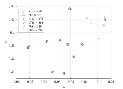
Figure 16: Sensitivity of the most unstable eigenvalues to the mesh resolution at $Re=60,000$, $\delta=0$.

As forthcoming results will show, simulating numerically this configuration near criticality becomes increasingly demanding as curvature effects grow. This difficulty culminates with the cylindrical rotor-stator configuration. A grid sensitivity test reported in Table 2 of the Appendix A shows that the leading eigenvalue responsible of the loss of stability of the base flow is very sensitive to the numerical resolution while the others are not (see fig.16). This confirms the observation made in ref.[19, 46] for a rotor-stator cavity with $\Gamma=10$. This test demonstrates that it is computationally demanding to claim spatial convergence with reasonable computing resources, whatever the spatial scheme used. Visual inspection reveals that the main difficulty deals with capturing the small vortical structures, for instance present even, quite unexpectedly, in the regular corner at $z=0,r=R_{2}$. As a compromise, all our investigations are carried out for a nominal resolution $N_{r}\times N_{z}=512\times 256$ with a uniform grid in $r$ and a cosine grid in $z$.

III Base flow, eigenmodes and linearised dynamics

III.1 Base flow

For each parameter $Re$ and $\delta$ the system of equations admits a steady axisymmetric solution denoted as the base flow. It is determined up to machine accuracy using the same standard Newton–Raphson solver as in Ref. [51]. The associated velocity field ${\bm{U}_{b}}(r,z)$ is axisymmetric but features three components. Its structure is displayed in figure 2(a,b). It combines a shear azimuthal flow with a recirculating meridional flow. For large enough $Re$ this meridional flow consists of a parallel Ekman layer next to the rotor and a spatially developing Bödewadt layer on the stator, with the flow directed respectively outwards and inwards.

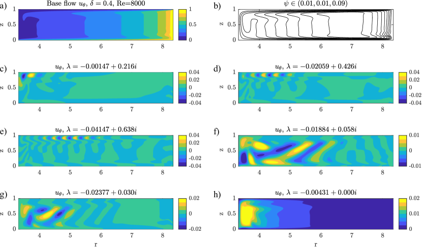
Figure 2: Base flow and related eigenvectors for $Re=8000$ and $\delta=0.4$. a) Azimuthal velocity $u_{\theta}(r,z)$ of the base flow b) corresponding meridional streamlines c) Azimuthal velocity $u_{\theta}(r,z)$ of the least stable eigenvector d)-h) other eigenvectors. In f) and g) inertial waves are visible.

III.2 Eigenspectrum and critical Reynolds number

The linear stability of this base flow can be monitored using the shift-and-invert method mentioned earlier. The eigenvalue problem involves an ansatz of the form ${\bm{u}}\sim e^{\lambda t}$, with $\lambda=\lambda_{r}+i\lambda_{i}$, so that a positive real part $\lambda_{r}>0$ indicates instability. A critical Reynolds number $Re_{c}$ can be defined where the real part of an eigenvalue (usually that with largest real part, but not only) vanishes. The critical values of $Re$ associated with the two dominant eigenvalues are shown in fig. 3(a) as a function of $\delta$ ranging from 0 to 1, with key values listed in Table 1. The corresponding imaginary part is reported in fig. 3(b), which allows one to distinguish branches. The family of eigenmodes labelled $B2$ is most unstable for all $\delta^{\prime}s$ between $\delta_{1}\approx 0.1$ and $\delta_{2}\approx 0.8$. Several points of codimension two, not studied in detail here, are visible as kinks along the branch. They suggest that branch $B2$ is not governed by a single individual branch of eigenvalues but rather consists of several of them. Near $\delta\rightarrow 0$, the data is consistent with a divergence of $Re_{c}$ as a power law of the form $Re_{c}=O(\delta^{-a})$ with $a\approx 2$. Between $\delta=0$ and $\delta<\delta_{1}$ another family of modes labelled $B1$ takes over as the most unstable. The dependence of $Re_{c}$ is affine in $\delta$, which leads to a finite value of $Re_{c}$ at $\delta=0$. In the interval $\delta\in(0,\delta_{1})$ the product $Re_{c}R_{2}$ is almost constant and equal to $3\times 10^{5}$. It is noted that Ref. [19] reports the value of $Re_{c}R_{2}=2.93\times 10^{5}$ for another aspect ratio of 10, hence this result may hold for intermediate values of $\Gamma$ too. This finite threshold is reported to our knowledge for the first time. In particular, it was not reported in previous investigations of rotor-stator flow with aspect ratio 5 in Ref. [17]. The branch B1 taking over between $\delta=\delta_{2}$ and $\delta=1$ supports frequencies vanishing linearly towards $\delta\rightarrow 1$ (we recall that time is in units of $H/R_{2}\Omega$). As $\delta\rightarrow 1$, the corresponding $Re_{c}$ diverges, at least using the current definition of $Re$.

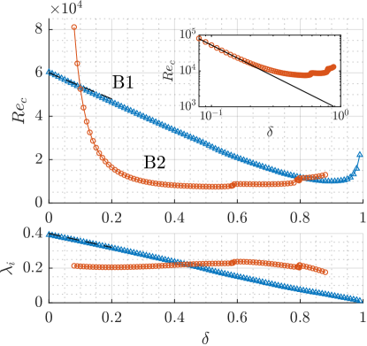
Figure 3: Critical Reynolds number $Re_{c}$ (top) and corresponding marginal eigenfrequency $\lambda_{i}$ (bottom) depending on the curvature parameter $\delta$. Branch B2 asymptotes to $Re_{c}=O(\delta^{-a})$ for $\delta\rightarrow 0$, with $a\approx 2$, which leads to a diverging threshold for the corresponding eigenmodes. On the other hand, continuation of the branch B1 leads to a finite value of $Re_{c}\approx 6\times 10^{4}$ for $\delta=0$, the corresponding eigenmode being shown in Fig. 4. Dashed lines plotted for $\delta<0.2$ and overlapping with branch B1 correspond to constant values of $ReR_{2}=3\times 10^{5}$ and $\lambda_{i}\,R_{2}=2$.

$\delta$	0.00	0.10	0.20	0.30	0.40	0.50	0.60	0.70	0.80	0.90	0.99
$\frac{R_{1}}{H}$	0.	0.55	1.25	2.14	3.33	5.	7.5	11.67	20.	45.	495.
$\frac{R_{2}}{H}$	5.	5.55	6.25	7.14	8.33	10.	12.5	16.67	25.	50.	500.
$Re_{c}$	59564	52573	16408	10054	8165	7572	8764	8646	11462	9960	22155
$\lambda_{i}$	0.392	0.211	0.205	0.209	0.218	0.226	0.238	0.226	0.216	0.042	0.011

Table 1: Values of non-dimensional inner and outer radius, critical Reynolds number $Re_{c}$ and corresponding marginal eigenfrequency $\lambda_{i}$ depending on the curvature parameter $\delta$. Approximate codimension-2 points are marked in bold. A sharp decrease of $\lambda_{i}$ at $\delta=0.1$ and $0.8$ corresponds to the switch from B1$\rightarrow$B2 and B2$\rightarrow$B1 respectively.

The azimuthal velocity of a few representative selected eigenmodes is shown in fig. 2. Azimuthal velocity fields typical of the eigenvectors from branch $B1$ are shown in fig. 4. The eigenmodes can grossly be classified into distinct categories depending on the spatial region where the velocity displays the largest amplitude :

• Bödewadt modes These modes are made of counter-rotating vortices located strictly inside the Bödewadt layer along the stator. Such modes have a non-zero phase velocity oriented inwards towards the rotation axis, hence they correspond to boundary layer modes propagating in the direction of the flow. The Bödewadt boundary layer grows spatially and the eigenfrequencies depend on the spatial localisation of the mode, as will be detailed in the next section. Such modes are shown in fig. 4(a) and also in fig. 2(c,d,e), with three frequencies forming a triad of the form $f_{1}=\pm f_{2}\pm f_{3}$

• Shift modes These steady modes are located in the bulk near the inner boundary at $r=R_{1}/H$, there where the velocity field was reported as self-similar [10]. Their importance has been noted for generic Hopf bifurcations [52], as such modes are in connection to the second order mean flow modification induced by self-interaction of the primary Hopf mode. Such a shift mode is shown in fig. 2(h)

• Shroud modes They correspond to streaks attached to the shroud. An example of a shroud mode is shown in fig. 4(c). This corner structure is analogous to the first instability mode in low aspect ratio cavities with adiabatic top and bottom walls [36, 40, 41, 42, 43, 45]

• Inertial bulk modes These modes are located exclusively in the bulk but unlike shift modes they also occur away from the rotation axis. These modes are propagating modes. They feature a patterned spatial structure with several clearly oblique wave vectors varying with radial location. Since the local rotation varies with the radius, these eigenmodes are labelled inertial by an incomplete analogy with inertial modes in a rotating fluid [1], however with locally varying angular speed [53]. When the rotation rates is spatially constant, inertial waves are known to propagate along directions making a constant angle with the rotation axis that depends only on their frequency. Large-scale gradients of rotation rate are expected to distort the wave pattern in such a way that for a given frequency the angle depends now on position. This is precisely observed in fig. 2(f), most clearly for $4\leq r\leq 7$ where the angle increases as the core rotation rate decreases with decreasing radius.

The topology and the classification of the modes of the branch $B1$ morphs, as $\delta$ moves from high values close to 1 down to 0, from shroud-localised modes to Bödewadt roll-like modes combined with inertial oscillations emitted from the roll part.

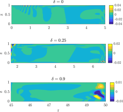
Figure 4: Azimuthal velocity of the neutrally stable eigenvector on the branch B1. Structure of the eigenvector evolves gradually from the rolls in the Bödewadt layer for $\delta=0$, through the structures of similar amplitude in two opposite corners of the cavity for $\delta=0.25$, to the corner structure near the shroud $\delta=0.9$. For the corresponding values of $Re_{c}$ and $\lambda_{i}$ see figure 3.

Unlike what fig. 3 could suggest, the competition does not involve solely $B1$ and $B2$. B1 was traced to show that it is a continuation of the same eigenmode which is most unstable at both end regions of variation of $\delta$, although, as fig. 4 shows, there seems to be little in common between the eigenmode structure at both ends. When B2 is first unstable, that is for $0.1\lesssim\delta\lesssim 0.8$, there are often many modes that become unstable before $Re$ is increased up to the value corresponding to the B1 curve. For instance, for $\delta=0.4$, the evolution of the spectrum in fig. 9 shows that for $Re=2\times 10^{4}$, there are as many as 15 other eigenmodes which are linearly unstable. This situation is common for all values of $\delta>0.3$. For $\delta<0.2$, however, B1 and B2 modes are the first ones to become unstable.

As mentioned in the introduction, additional variability comes from the nature of the boundary conditions for the velocity on the inner hub and outer shroud. The values of $Re_{c}$ are documented, for the case of $\delta=0.5$, for various types of boundary conditions. The comparison is shown in Table 3 in Appendix B.

III.3 Radial localisation

When computing the eigenspectrum of the system linearised around the steady base flow solution, an original property emerged for all $\delta<1$. It is best seen in Fig. 5 where eigenvectors, associated with the eigenvalues of largest real part, are plotted implicitly in the plane $(r,\lambda_{i})$, where $\lambda_{i}$ is the imaginary part of a complex eigenvalue $\lambda$. More precisely, the kinetic energy of each eigenvector, which is independent of its phase, is considered at axial position $z=z^{*}$ with $z^{*}=0.94$ (next to the stator) and plotted radially. In this $(r,\lambda_{i})$ representation, each eigenspectrum appears as a coherent rectilinear beam-like shape stretching from the hub towards the shroud as $\lambda_{i}$ increases.

The direct interpretation is that all eigenvectors with spatial support localised inside the Bödewadt layer see their active region localised radially at a position depending only on the value of the angular frequency $\lambda_{i}$. This makes radial localisation the signature of a given eigenmode (or rather of its natural oscillation frequency). For a subset of eigenvectors from fig. 5 corresponding to $\lambda_{i}>0.3$ the phase speed of the waves constituting the eigenvector was computed as the ratio between the oscillation angular frequency $\omega$ and the local radial wave number $k$ obtained from a spatial Fourier transform in $r$ at $z=z^{*}$. This phase speed is compared against the local maximal radial speed in the Bödewadt layer in figure 6, showing an unambiguous linear dependence between them. This correlation between wave speed and radial velocity is more marked when $\delta$ is far from 1. This is consistent with the fact that for $\delta\rightarrow 1$ there is no curvature of the base flow, and hence no large scale radial velocity gradient.

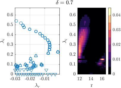
Figure 5: Spectrum of linearised Navier–Stokes operator and radial support of all (normalised) eigenmodes parametrised by their eigenfrequency $\lambda_{i}$ (amplitude of $u_{\theta}(z=z^{*})$ for $z^{*}=0.94$ ) at Re=8000 for $\delta=0.4$ (a) and at Re=8500 for $\delta=0.7$. The center of mass of the spatial support varies linearly with $\lambda_{i}$ (for $\lambda_{i}>0.2$). Eigenvectors from figure 2 correspond to red crosses in (a). Spectrum is obtained using series of shifts in Arnoldi method and plotted using different symbols.

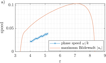
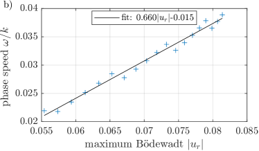
Figure 6: Comparison of the maximal radial velocity associated to the base flow and the local phase speed of the waves corresponding to the eigenvectors of the base flow (cf. fig. 5) for Re=8000 and $\delta=0.4$. In (a) both phase speed and a local radial base flow velocity are plotted as the function of $r$. In (b) the linear fit shows that in the current configuration the wave speed is a linear function of the local maximal radial base flow velocity equal $40\%\ -\ 50\%$ of the local maximal radial base flow velocity.

III.4 Non-normal amplification

Linear stability analysis of the base flow, via the listing of unstable eigenvalues, represents only partial knowledge of the stability of the problem. As is well known from investigations of shear flows, the finite-time stability of the system with respect to infinitesimal perturbations to the base flow is also of interest. In particular, if the operator resulting from the linearised equations is non-normal (i.e. it does not commute with its adjoint), finite-time amplification of the perturbation energy $E(t)=\int|{\bm{u}^{\prime}}|^{2}d^{3}x$ is possible, where ${\bm{u}^{\prime}}={\bm{u}}-{\bm{U}_{b}}$.

In principle, optimal growth can be investigated using the toolbox presented in ref. [54]. We preferred the more economical non-optimal approach of i) considering one generic enough initial condition and ii) monitoring the energy amplification associated with that initial condition (computed using standard time-stepping of the linearised equations). This is achieved using an initial condition $u^{\prime}_{\theta}$ consisting of a random field of small amplitude. The energy gain

$$G(t)=\max_{t\geq 0}\frac{E(t)}{E(0)}$$ (4)

is plotted in fig. 7 versus $Re$ and $\delta$, focusing only on the values of $\delta\leq 0.5$.

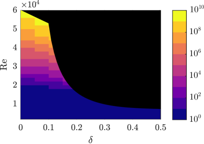
Figure 7: Energy gain $G$ in logarithmic scale as a function of $\delta$ and $Re$ (see eq.(4)), where G is the maximal energy amplification by the linearised dynamics for a given random perturbation. For low $\delta$, large gain values are a consequence of the non-normality of the underlying linear operator. The part of the ($\delta,Re$) space corresponding to a linearly unstable base flow (cf. fig. 3) is filled with black.

Fig. 7 shows clearly that $G$ increases fast with $Re$. For each individual value of $\delta$, the data is compatible with a fit of the form $G=e^{aRe}$. Between $\delta=0.5$ and $\delta=0$, the value of $G$ at $Re=Re_{c}$ increases by almost 10 decades. If we follow the neutral curve $Re_{c}(\delta)$ towards $\delta=0$, the global tendency is a sharp rise of $G$ especially for $\delta\leq 0.15$. Strong non-normal growth implies rapid Lyapunov divergence between state space trajectories. In particular, even if a stable supercritical branch of nonlinear solutions exists close to a bifurcation, strong non-normality can make the branch unreachable by time-stepping in practice, as discussed extensively in Ref. [19].

IV Nonlinear rolls dynamics

IV.1 Pairing mechanism reinterpreted

The spatial localisation property of the eigenmodes, highlighted in fig. 5, has important consequences on the dynamics of the rolls, even in nonlinear unsteady regimes. Evidence for this is analysed in detail in the case $\delta=0.4$, a parameter for which the base flow first loses stability at $Re_{c}\approx 8,165$ in favour of the mode $B2$. The instability was found to be supercritical and the flow saturates nonlinearly, for $Re\gtrsim Re_{c}$ , to a periodic flow. As the primary eigenmode saturates in amplitude, the generation of harmonics of higher frequency leads to remarkable spatial dynamics.

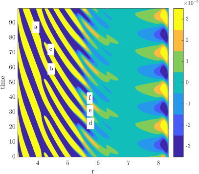
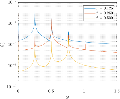
Figure 8: Space–time diagram of the fluctuation $(u_{\theta}-<u_{\theta}>)(r,z^{*},t)$ at $z=z^{*}=0.94$, for $\delta=0.4$ and $Re=13,000$. Left: snapshot of $u_{\theta}$ fluctuation velocity contour. Two structures (b,c) merge into one (a) at $r=3$ while three structures (d,e,f) merge into two (b,c) at $r=4$. Right : angular frequency amplitude spectra from azimuthal velocity probes at three positions $r=3.96,4.58,5.83$, $\tilde{r}=(r-R_{1})/(R_{2}-R_{1})$. The dashed line marks the frequency of the primary mode $\omega\approx 0.2545$.

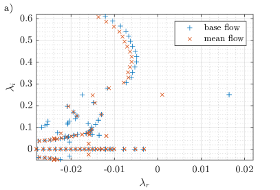
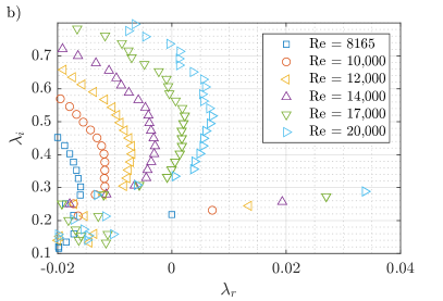
Figure 9: Spectrum of the Navier–Stokes operator linearised around the base flow and the base flow for Re=13,000 (a) and for different Re (b) at $\delta=0.4$. The real part of the most unstable eigenvalue is reduced where the linearisation point is switched from the base flow to the mean flow of nonlinearly saturate branch. This is consistent with the RZIF property.

Fig. 8 shows a space-time diagram of the azimuthal velocity fluctuation along one given radial line inside the Bödewadt layer (at $z=z^{*}$) for $Re=13,000$ where roll pairing events can be observed. At approximately mid-radius streaky structures are seen to propagate inwards, forming a front near $r\approx 6$. Between locations $r\approx 6-8$ and $r\approx 4.5-5.5$ the dominant angular frequency of the oscillations inside the front changes in a ratio 2/3 from $\omega\approx 0.76$ to $\omega=0.51$. Moving further inwards down to $r\lesssim 4$, it decreases again to $\omega\approx 0.254$, one half of the angular preceding frequency, as found from velocity spectra at various locations in fig.8. We note that for this configuration the primary, most unstable mode has an eigenvalue $0.0181+0.2545i$, which is exactly the angular frequency $\omega_{1}=0.2545$ identified closest to the axis in fig. 8. The dynamics of roll merging, as seen in fig. 8, can be explained as follows. The primary mode of angular frequency $\omega_{1}$ generates nonlinearly a second harmonic of angular frequency $2\,\omega_{1}$. This oscillation excites, among the modes in the spectrum, one of the eigenmodes with angular frequency closest to $2\,\omega_{1}$, belonging to the continuous like branch visible in fig. 9. Because of its higher frequency, that eigenmode has its spatial support located upstream of the primary mode, as shown in fig.5. The spatial coexistence of two different frequencies is interpreted as roll pairing and a pairing appears there where both modes are of comparable amplitude. The story repeats itself through the nonlinear generation of a $3\>\omega_{1}$ forcing which makes an eigenmode of frequency close to $3\>\omega_{1}$ resonate. Since the corresponding mode is located further upstream, a second pairing event appears. At the location corresponding to (d,e,f) in fig. 8, one roll out of three disappears. In general, for this phenomenological start of a cascade to become visible, the amplitude of the primary mode has to be large enough to induce second and third harmonics sufficiently large to make the corresponding modes visible. This explains why $Re$ has to be increased to a large supercritical value ($1.3\times 10^{4}$) well above $Re_{c}\approx 8,165$. We checked that, despite this large distance from criticality, the corresponding base flow has still only one unstable mode (see fig. 9(a)).

The spectrum of the operator linearised around the mean flow (computed by long time integration) was also computed, inspired by Ref. [55]. As seen in fig. 9(a), the mean flow is, in a first approximation, neutrally stable. It can thus be considered as belonging marginally to the class of flows sharing the RZIF property [56, 57], although the frequency of the mean flow is very little displaced from that of the base flow. Beyond that level of approximation, the non-strictly zero value of $\lambda_{r}$ is a signature of the non-negligible amplitudes associated with harmonics. Let us also mention that the visibility of this pairing mechanism is sensitive to the choice of boundary condition on the shroud. Pairing is more easily visible when the shroud is attached to the stator as in the experiments by Schouveiler et al. [14], or with a linear azimuthal velocity profile as in the numerical simulations reported in [22].
We again emphasize the crucial role of the radial dependence of the radial velocity in the Bödewadt layer in the reported phenomenology. Its key ingredients are the constant ratio between the phase velocity and the maximum velocity and the affine dependence of the velocity on radius. This is illustrated in fig. 6 which results in the spatial localisation of the higher frequency eigenmodes illustrated in fig. 5.

The phenomenology described above constitutes an alternative explanation to the linear multi-harmonics forcing considered in [21]. Both mechanisms are an illustration of the pairing phenomenon. They are however not in direct competition since one phenomenon occurs only at high $Re$ and for high amplitudes, whereas the other holds for all $Re$. The only difference between the two mechanisms concerns the way higher harmonics are generated : in one scenario they are a consequence of the nonlinear term in the governing equations, whereas in the other the higher harmonics are explicitly introduced as part of a multi-harmonic forcing.

IV.2 Coexistence of nonlinear regimes

The time-periodic regime described above for $\delta=0.4$ was identified as the only attractor of the system for the parameters chosen. As $\delta$ is decreased, bistability is found, meaning that the attracting state depends on the initial condition. This is illustrated in fig. 10 for the case $\delta=0.12$, $Re=55,000$. For $\delta=0.12$, $Re_{c}=37,530$, is associated with a critical angular frequency of $0.208$; for $Re=55,000$ linearisation around the base flow yields only one unstable eigenvalue $0.013+0.232i$. In the first row of fig. 10 a time-periodic regime, qualitatively similar to that for $\delta=0.4$, is uncovered. It also features a primary mode with angular frequency $\omega_{1}$ accompanied by two harmonics $2\,\omega_{1}$ and $3\,\omega_{1}$. However, pairing is not observed in the corresponding space-time diagram, which suggests that the amplitudes of these harmonics, although visible in the frequency spectrum, are not as strong as for the parameters in Subsection IV.1.

For strictly the same parameters, another attracting state is found by starting the simulation from a different initial condition, shown in the lower row of fig. 10. The corresponding frequency spectrum is broadband with no preferred frequency, the standard signature of deterministic chaos. Close to the hub, spectral amplitudes follow an exponential law. For the most outwards radii, the frequency spectrum shows most of the energy concentrated near angular frequencies $\omega=0$ and $\omega\approx 1$, but unlike the supercritical case discussed above, no simple interpretation is terms of eigenmodes can be given. No dynamical origin for this chaotic state could be found. In analogy with the attractors found in linearly stable shear flows [58], it is apparently disconnected from the base flow, meaning that it does not emerge from the amplitude saturation of an unstable eigenmode.

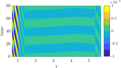
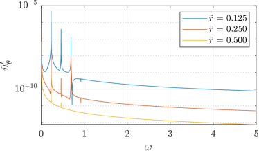
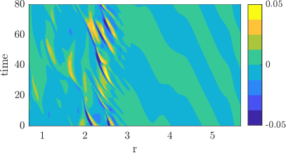
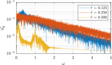
Figure 10: Space time diagrams (left) and corresponding spectra of probe signal (right) for $\delta=0.12$ at $Re=55,000$ for the periodic solution (top) and the chaotic solution (bottom). It is noteworthy that two solutions exist at exactly the same value of the governing parameters $Re$ and $\delta$. Therefore, depending on the initial condition for the time integration, either of the two states can be reached. For this configuration $Re_{c}=37530$ and the angular frequency of the neutral mode is $\lambda_{i}=0.208$. At $Re=55000$ this eigenvalue shifts to $\lambda=0.013\pm 0.232i$.

IV.3 Rotor stator case $\delta=0$.

IV.3.1 Large-amplitude branch

Our initial aim was to catch solutions belonging to the supercritical branch emanating from $Re_{c}$ by using the nonlinear timestepping code. By doing so we uncovered a disconnected branch of chaotic solutions that can be continued to $Re$ even below $Re_{c}$.

The evolution of the $L_{2}$ norm of the perturbation reported in fig. 11 shows that, starting from an initial perturbation of amplitude $10^{-10}$ and after the initial non-normal growth, the norm of the perturbation decreases to $10^{-9}$ before it starts to increase exponentially with a growth rate that agrees with the linear stability analysis. After this phase of exponential growth the solution starts to grow faster than exponential and ends up eventually on a large amplitude branch characterised by unsteady chaotic fluctuations and a broadband frequency content (not shown). The fact that the solution ends up on a chaotic branch is not due to non-normal growth, rather to the fact that the supercritical branch emanating at $Re_{c}$, if any, folds back rapidly, and does not exist for $Re=6\times 10^{4}$. This situation is exactly the same at that reported in [19] for $\Gamma=10$, where the supercritical branch was found to exist only for $(Re-Re_{c})<10^{-3}$ before folding back subcritically. Starting from this chaotic solution $Re$ was progressively decreased in order to locate the nose, in other words the tipping point of this large amplitude subcritical branch. It was found to lie in the interval $3.3\times 10^{4}<Re<3.4\times 10^{4}$. Surprisingly, just before this point, a periodic solution was identified for $Re=3.4\times 10^{4}$. Its period is $T=18,6$. The corresponding space-time diagram is shown in fig.12(a). This periodic solution might be misinterpreted as belonging to a supercritical branch, which is clearly not the case since $Re$ is below $Re_{c}$ (see Table 1).

Comparing the time-periodic regime in fig. 12(left) to the chaotic regime in fig. 12(right) at slightly higher $Re$, we see that the rolls are closer to the axis in the periodic regime. In the chaotic regime the propagation velocity fluctuates from roll to roll. Even closer to the axis for $1\leq r\leq 2$ subharmonic frequency can be observed. This chaotic regime compares favourably to the one shown in fig. 10 for non-zero $\delta$, yet higher $Re=55,000$, and without the subharmonic frequency reported at $\delta=0$ and smaller $Re$. As shown in Ref. [19] for larger $\Gamma$, the maximum amplitude of the rolls corresponds to locations where fluid is ejected from the Bödewadt layer towards the bulk. Closer examination of the velocity field suggests that these ejections contribute to the sustainment of the inertial oscillations in the bulk.

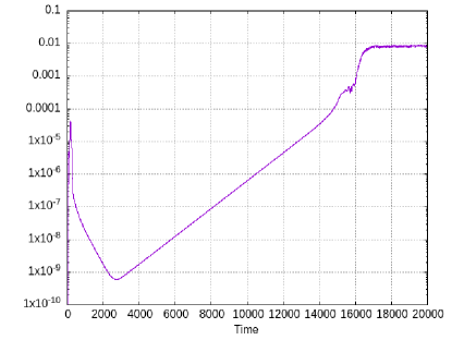
Figure 11: Time evolution of the $L_{2}$ norm of $v_{\theta}$; $Re=6\times 10^{4}$, $\delta=0$.

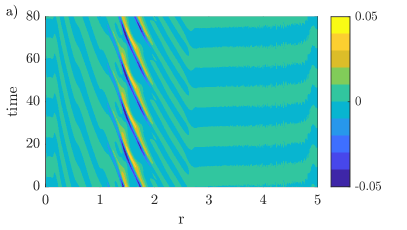
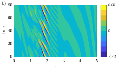
Figure 12: Space–time diagram of the fluctuation $(u_{\theta}-<u_{\theta}>)(r,z^{*},t)$ for $\delta=0$ at $z=z^{*}=0.94$. a) : periodic regime ($Re=34,000$), b) : chaotic regime ($Re=37,000$).

IV.3.2 Edge state

For the case $\delta=0$, additional nonlinear computations of edge states have been performed, with the goal to list the most important finite-amplitude states for a bifurcation diagram to be drawn. Edge states [59] are unstable states attracting the trajectories constrained on the laminar basin boundary. They exist in typically subcritical conditions, including when the top branch is disconnected from the (linearly stable) base flow solution. These edge states are computed starting from the base flow solution, to which a given and reproducible azimuthal velocity perturbation is added, whose amplitude is recursively tuned such that the simulation evolves neither towards the laminar base flow nor towards the chaotic state. For $Re=5\times 10^{4}$ the edge state is quasi-periodic in time (fig.13) with two incommensurate frequencies. This result is similar to the edge computation carried out for an aspect ratio of 10 [19]. For $Re=4\times 10^{4}$ the edge state, however, is strictly periodic in time (fig. 14) with less intense fluctuations and a period $T\approx 24.8$. These computations confirm the subcriticality of the state appearing at $Re_{SN}\approx 3.2\times 10^{4}$. The bifurcation leading from the quasi-periodic to the periodic edge state might be of Neimark-Sacker type, or might correspond to synchronisation inside an Arnold’s tongue, but this has not been investigated further.

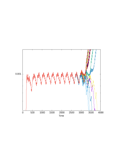
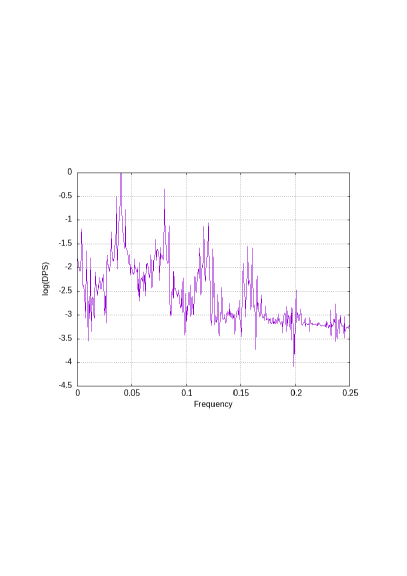
Figure 13: Trajectories bracketing an edge trajectory for $Re=5\times 10^{4}$, $\delta=0$: (left) time evolution of the $L_{2}$ norm of fluctuating $v_{\theta}$ ; (right) power spectrum of corresponding pointwise azimuthal velocity, sample of 16384 points over time length of 1634.4 starting at t=1000. The trajectories shown approximate the edge state for $1000\leq t\leq 2500$. $L_{2}$ norm of amplitude of initial noise is $7.6\times 10^{-8}$.

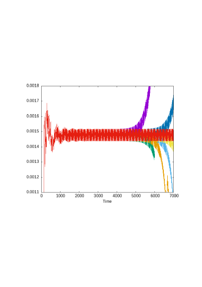
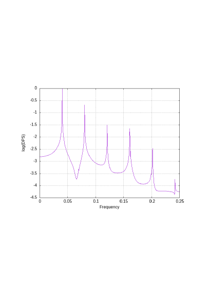
Figure 14: Trajectories bracketing an edge trajectory for $Re=4\times 10^{4}$, $\delta=0$ : (left) time evolution of the $L_{2}$ norm of fluctuating $v_{\theta}$ ; (right) power spectrum of corresponding pointwise azimuthal velocity, sample of 32768 points over time length of 3276.8. The trajectory in red approximates the edge state for $2000\leq t\leq 7000$. $L_{2}$ norm of amplitude of initial noise is $1.9\times 10^{-9}$.

V Bifurcation sequences : from supercritical to subcritical in $Re$

We now compile here the lessons learned from the computation of $Re_{c}$ for all $\delta^{\prime}s$ and from a series of numerical explorations of nonlinear regimes at various parameter values. Our observations yield a qualitative description, as $\delta$ is reduced, of the sequences of bifurcations leading to unsteadiness as $Re$ increases.

We chose to start the description of the various regimes at $\delta=0.4$ and to decrease $\delta$ from there towards the rotor-stator case at $\delta=0$. The different cases are summarized in fig. 15.

• At $\delta=0.4$, the transition to unsteadiness is supercritical : for $Re<Re_{c}$ the only stable state is the base flow while for $Re>Re_{c}$ the base flow is unstable and the system evolves towards the complex dynamics described in fig. 8 (red branch in fig. 15a) showing the ($\omega$,$2\,\omega$,$3\,\omega$) pairing as described in section IV.1. There are many secondary bifurcations points in between $Re_{c}(B2)$ and $Re_{c}(B1)$. At $Re=1.5\times 10^{4}$, the solution on the supercritical branch becomes quasiperiodic, and chaotic at larger $Re$.

• For $\delta=0.15$, the most unstable branch emerging at $Re_{c}$ and based on $B2$ (red in fig. 15b), still emerges supercritically, followed by a second destabilising branch (blue). Note that the two corresponding values of $Re_{c}$ increase as $\delta$ decreases. Attempts to find a large amplitude branch for increasing values of $Re$ up to $7\times 10^{4}$ remained unsuccessful.

• For $\delta=0.12$ the situation is relatively similar to $\delta=0.15$, except that the critical values of $Re$ have moved up in $Re$, and for the notable apparition of the disconnected branch at values of $Re$ comparable to $Re_{c}$. As a result, the complex dynamics on the upper branch is now in direct competition with the supercritical dynamics, both displayed in fig.10. There is even a properly subcritical interval for $Re>35,000$ where the disconnected branch is in competition with the stable base flow below $Re_{c}=37784$.

• The case $\delta=0$ follows from the simple continuation to lower $\delta$ of the former cases. The critical value for the mode $B1$ has moved to a relatively high value $Re_{c}\approx 6\times 10^{4}$ while that for $B2$ has diverged. A direct search for supercritical solutions at slightly supercritical value of $Re$ lead instead to the large amplitude branch, confirming the result that this branch, if supercritical, is virtually unreachable. The large amplitude branch extends to values of $Re$ around $3.2\times 10^{4}$ and ends in what appears to be a saddle node fold. Just before a time-periodic solution is found for $Re=3.5\times 10^{4}$. Edge states are found on the border of the attraction basin between the base flow and the large amplitude branch. The edge state identified ($Re=4\times 10^{4}$) close to the tipping is found to be periodic in time whereas that found for $Re=5\times 10^{4}$ is biperiodic, just like for $\Gamma=10$ [19].

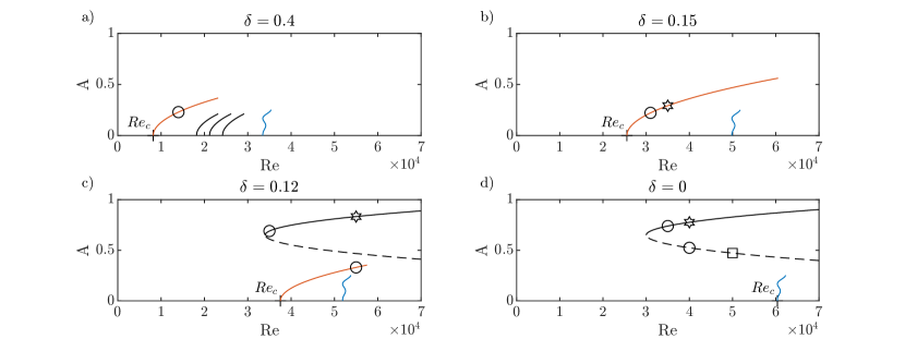
Figure 15: Sketch of the evolution of the bifurcation diagrams for selected values of $\delta$. Branches in red correspond to a B2 eigenmode while those in blue to a B1 eigenmode. Additional symbols are confirmed solutions (periodic $\circ$, quasi-periodic $\square$, chaotic $\bigstar$; two edge states at $\delta=0$, top branch state and the supercritical branch state at $\delta=0.12$, supercritical branch as in figure 8 at $\delta=0.4$). The global transition picture switches from supercritical to subcritical as $\delta$ is decreased. The amplitude $A$ is arbitrary and not to scale.

VI Conclusions

We have considered the axisymmetric flow inside an annular duct with a rotating disk, governed by a Reynolds number $Re$ and a geometric homotopy parameter $\delta$. In this system, the $\delta\rightarrow 0$ limit corresponds to axisymmetric hub-free rotor-stator flow while the $\delta\rightarrow 1$ limit corresponds to a flow analog to a two-dimensional differentially heated cavity. A description of the transition scenario in $Re$ as $\delta$ decreases is given together with results from linear stability theory as well as with quantitative estimations of non-normal amplification. A plausible scenario of minimal complexity is suggested in Fig. 15. As $\delta$ decreases towards zero, the dynamics switches from supercritical to subcritical in $Re$, both because the threshold values of $Re_{c}$ for the destabilisation of global modes increase, and because the onset $Re_{SN}$ of the competing disconnected state occurs at lower and lower values of $\delta$. For low enough $\delta$, the amplification of disturbances due to non-normal effects is strong enough so that the supercritical branches are not reachable in practice in direct simulations. The disconnected state becomes hence in practice the only attractor for $Re>Re_{SN}$.

The observations compiled above lead to a more complete picture of the axisymmetric transition scenario for the rotor-stator case at $\delta=0$ with an aspect ratio of 5. The base flow loses its stability at a finite value of $Re_{c}\approx 6\times 10^{4}$, not identified in previous numerical investigations of [17], since restrained to lower values of $Re$. Identifying this critical value would have been virtually impossible with the sole use of a nonlinear time-stepping code. Nevertheless this linear instability and the steep supercritical branch emanating at $Re_{c}$ are relatively exotic : non-normality will amplify almost any initial disturbance up to levels where they transition to the disconnected state, whether for $Re$ above or below $Re_{c}$, as soon as $Re\gtrsim Re_{SN}~(\approx 3.3\times 10^{4})$. This brings the phenomenology very close to that encountered in other shear flows such as pipe flow or plane Couette flow [58]. The disconnected state, together with the edge state as its unstable counterpart, was found to be either chaotic or time-periodic close to the tipping point, whereas the edge state was found either quasiperiodic or also time-periodic closer to the tipping point. If we compare now to the bifurcation diagram obtained recently in Ref.[19] for a rotor-stator of aspect ratio 10, many similarities can be found, notably the subcriticality of the disconnected state, but also the large non-normal amplification observed at high $Re$ values comparable to $Re_{c}$ and the associated consequences. Several interesting differences are noted however, for instance finite lifetimes of the chaotic state were not identified in the current simulations. As another difference with the case $\Gamma=10$ we reported the occurrence of coexisting time-periodic and chaotic solutions as well as of time-periodic states on both the upper stable and lower unstable disconnected branch. These periodic states should be amenable to numerical continuation using arclength techniques, which is the subject of ongoing work. It would be interesting to see which of the conclusions of the present study apply also to the description of the three-dimensional transition process.

Appendix A

$N_{r}\times N_{z}$	$\delta=0$		$\delta=0.1$
	$Re_{c}$	$\omega$	$Re_{c}$	$\omega$
512 $\times$ 256	59564	0.3924	47941	0.3942
768 $\times$ 384	58217.5	0.4052	46602	0.404
1152 $\times$ 576	57874.5	0.4116	46324.5	0.409
1728 $\times$ 864	57817	0.4146	46260.5	0.4112

Table 2: Grid convergence $\delta=0$ B1 (left) and $\delta=0.1$ B1 (right).

Appendix B

$BC_{R1}$	$BC_{R2}$	$Re_{c}$	$\lambda_{i}$
ROT	FIX	4030	0.36
LIN	LIN	5315	0.3565
STF	FIX	5833	0.211
STF	LIN	6462	0.4229
STF	STF	7666	0.2255
STF	ROT	7572	0.2266
FIX	ROT	8020	0.2108

Table 3: Critical Reynolds number $Re_{c}$ and angular frequency of most unstable eigenmode $\lambda_{i}$ for various velocity boundary conditions on the inner hub $BC_{R1}$ and outer shroud $BC_{R2}$ ; $\delta=0.5$ ; STF = stress-free ; ROT = rotating ; FIX = null velocity ; LIN = linear profile for the azimuthal velocity as a function of $z$. The reported values of $Re_{c}$ show that the most stable configuration corresponds to a steady hub and rotating shroud whereas the least stable is the rotating hub and steady shroud, with a factor two in $Re$ between these two extremes.

References

- Greenspan [1969] H. P. Greenspan, The theory of rotating fluids (Cambridge University Press, 1969).
- Pedlovski [1987] J. Pedlovski, Geophysical fluid dynamics, 2nd ed. (Springer New York, NY, 1987).
- Owen and Rogers [1989] J. Owen and R. Rogers, Flow and Heat Transfer in Rotating-Disc Systems : Rotor-stator systems, volume 1, 1st ed. (Springer-Verlag, Berlin, 1989).
- Dijkstra and Van Heijst [1983] D. Dijkstra and G. J. F. Van Heijst, The flow between two finite rotating disks enclosed by a cylinder, J. Fluid Mech. 128, 123 (1983).
- Adams and Szeri [1982] M. L. Adams and A. Z. Szeri, Incompressible flow between finite disks, J. Appl. Mech. 49, 1 (1982).
- Szeri et al. [1983] A. Z. Szeri, S. J. Schneider, F. Labbe, and H. N. Kaufman, Flow between rotating disks. Part 1. Basic flow, J. Fluid Mech. 134, 103 (1983).
- Brady and Durlofsky [1987] J. F. Brady and L. Durlofsky, On rotating disk flow, J. Fluid Mech. 175, 363 (1987).
- Oliveira et al. [1991] L. A. Oliveira, J. Pecheux, and A. O. Restivo, On the flow between a rotating and a coaxial fixed disc: numerical validation of the radial similarity hypothesis, Theoret. Comput. Fluid Dynamics 2, 211 (1991).
- Batchelor [1951] G. K. Batchelor, Note on a class of solutions of the Navier-Stokes equations representing steady rotationally-symmetric flow, Q. J. Mech. Appl. Math. 4, 29 (1951).
- Cousin-Rittemard et al. [1999] N. Cousin-Rittemard, O. Daube, and P. Le Quéré, Structuration de la solution stationnaire des écoulements interdisques en configuration rotor–stator, C. R. Acad. Sci., Ser. II b 327, 221 (1999).
- Launder et al. [2010] B. Launder, S. Poncet, and É. Serre, Laminar, transitional, and turbulent flows in rotor-stator cavities, Ann. Rev. Fluid Mech. 42, 229 (2010).
- Martinand et al. [2023] D. Martinand, E. Serre, and B. Viaud, Instabilities and routes to turbulence in rotating disc boundary layers and cavities, Philos. Trans. Royal Soc. A 381, 20220135 (2023).
- Xie et al. [2024] Y. Xie, Q. Du, L. Xie, Z. Wang, and S. Li, Onset of turbulence in rotor–stator cavity flows, J. Fluid Mech. 991, A3 (2024).
- Schouveiler et al. [1999] L. Schouveiler, P. Le Gal, M. P. Chauve, and Y. Takeda, Spiral and circular waves in the flow between a rotating and a stationary disk, Exp. Fluids 26, 179 (1999).
- Gauthier et al. [1999] G. Gauthier, P. Gondret, and M. Rabaud, Axisymmetric propagating vortices in the flow between a stationary and a rotating disk enclosed by a cylinder, J. Fluid Mech. 386, 105 (1999).
- Serre et al. [2001] É. Serre, E. Crespo Del Arco, and P. Bontoux, Annular and spiral patterns in flows between rotating and stationary discs, J. Fluid Mech. 434, 65 (2001).
- Lopez et al. [2009] J. M. Lopez, F. Marques, A. M. Rubio, and M. Avila, Crossflow instability of finite Bödewadt flows: Transients and spiral waves, Phys. Fluids 21 (2009).
- Daube and Le Quéré [2002] O. Daube and P. Le Quéré, Numerical investigation of the first bifurcation for the flow in a rotor–stator cavity of radial aspect ratio 10, Comput. Fluids 31, 481 (2002).
- Gesla et al. [2024a] A. Gesla, Y. Duguet, P. Le Quéré, and L. Martin Witkowski, Subcritical axisymmetric solutions in rotor-stator flow, Phys. Rev. Fluids 9, 083903 (2024a).
- Schouveiler et al. [2001] L. Schouveiler, P. Le Gal, and M. P. Chauve, Instabilities of the flow between a rotating and a stationary disk, J. Fluid Mech. 443, 329 (2001).
- Gesla et al. [2024b] A. Gesla, Y. Duguet, P. Le Quéré, and L. Martin Witkowski, On the origin of circular rolls in rotor-stator flow, J. Fluid Mech. 1000, A47 (2024b).
- Cousin-Rittemard [1996] N. Cousin-Rittemard, Contribution à l’étude des instabilités des écoulements axisymétriques en cavité inter-disques de type rotor-stator, Ph.D. thesis, Univ. Paris VI, Paris, France (1996).
- Do et al. [2010] Y. Do, J. M. Lopez, and F. Marques, Optimal harmonic response in a confined Bödewadt boundary layer flow, Phys. Rev. E 82, 036301 (2010).
- Serre et al. [2004] E. Serre, E. Tuliszka-Sznitko, and P. Bontoux, Coupled numerical and theoretical study of the flow transition between a rotating and a stationary disk, Phys. Fluids 16, 688 (2004).
- Tuliszka-Sznitko and Zielinski [2005] E. Tuliszka-Sznitko and A. Zielinski, Numerical investigation of the nature of the first bifurcation for the flow in an annular rotor/stator cavity, J. Theor. Applied Mech. 43, 135 (2005).
- Severac et al. [2007] E. Severac, S. Poncet, E. Serre, and M.-P. Chauve, Large eddy simulation and measurements of turbulent enclosed rotor-stator flows, Phys. Fluids 19, 1 (2007).
- Poncet et al. [2009] S. Poncet, É. Serre, and P. Le Gal, Revisiting the two first instabilities of the flow in an annular rotor-stator cavity, Phys. Fluids 21 (2009).
- Makino et al. [2015] S. Makino, M. Inagaki, and M. Nakagawa, Laminar-turbulence transition over the rotor disk in an enclosed rotor-stator cavity, Flow Turb. Comb. 95, 399 (2015).
- Bridel-Bertomeu et al. [2017] T. Bridel-Bertomeu, L. Y. M. Gicquel, and G. Staffelbach, Large scale motions of multiple limit-cycle high Reynolds number annular and toroidal rotor/stator cavities, Phys. Fluids 29, 065115 (2017).
- Queguineur et al. [2019] M. Queguineur, T. Bridel-Bertomeu, L. Gicquel, and G. Staffelbach, Large eddy simulations and global stability analyses of an annular and cylindrical rotor-stator cavity limit cycles, Phys. Fluids 31, 1 (2019).
- Nagata [1990] M. Nagata, Three-dimensional finite-amplitude solutions in plane Couette flow: bifurcation from infinity, J. Fluid Mech. 217, 519 (1990).
- Clever and Busse [1992] R. M. Clever and F. H. Busse, Three-dimensional convection in a horizontal fluid layer subjected to a constant shear, J. Fluid Mech. 234, 511 (1992).
- Faisst and Eckhardt [2000] H. Faisst and B. Eckhardt, Transition from the Couette-Taylor system to the plane Couette system, Phys. Rev. E 61, 7227 (2000).
- Ishida et al. [2017] T. Ishida, Y. Duguet, and T. Tsukahara, Turbulent bifurcations in intermittent shear flows: from puffs to oblique stripes, Phys. Rev. Fluids 2, 073902 (2017).
- Veronis [1970] G. Veronis, The analogy between rotating and stratified fluids, Ann. Rev. Fluid Mech. 2, 37 (1970).
- Le Quéré and Behnia [1998] P. Le Quéré and M. Behnia, From onset of unsteadiness to chaos in a differentially heated square cavity, J. Fluid Mech. 359, 81 (1998).
- Henkes and Hoogendoorn [1990] R. Henkes and C. Hoogendoorn, On the stability of the natural convection flow in a square cavity heated from the side, Applied Scientific Research 47, 195 (1990).
- Xin and Le Quéré [2001] S. Xin and P. Le Quéré, Linear stability analyses of natural convection flows in a differentially heated square cavity with conducting horizontal walls, Phys. Fluids 13, 2529 (2001).
- Gadoin et al. [2001] E. Gadoin, P. Le Quéré, and O. Daube, A general methodology for investigating flow instabilities in complex geometries: application to natural convection in enclosures, Int. J. Numer. Meth. Fluids 37, 175 (2001).
- Xin and Le Quéré [2002] S. Xin and P. Le Quéré, An extended Chebyshev pseudo-spectral benchmark for the 8: 1 differentially heated cavity, Int. J. Numer. Meth. Fluids 40, 981 (2002).
- Xin and Le Quéré [2006] S. Xin and P. Le Quéré, Natural-convection flows in air-filled, differentially heated cavities with adiabatic horizontal walls, Numer. Heat Transfer A 50, 437 (2006).
- Xin and Le Quéré [2012] S. Xin and P. Le Quéré, Stability of two-dimensional (2D) natural convection flows in air-filled differentially heated cavities: 2D/3D disturbances, Fluid Dyn. Res. 44, 031419 (2012).
- Oteski et al. [2015] L. Oteski, Y. Duguet, L. Pastur, and P. Le Quéré, Quasiperiodic routes to chaos in confined two-dimensional differential convection, Phys. Rev. E 92, 043020 (2015).
- Net and Sanchez Umbria [2017] M. Net and J. Sanchez Umbria, Periodic orbits in tall laterally heated rectangular cavities, Phys. Rev. E 95, 023102 (2017).
- Khoubani et al. [2024] A. Khoubani, A. V. Mohanan, P. Augier, and J. B. Flór, Vertical convection regimes in a two-dimensional rectangular cavity: Prandtl and aspect ratio dependence, J. Fluid Mech. 981, A10 (2024).
- Gesla [2024] A. Gesla, Numerical investigation of the dynamics of an axisymmetric rotor-stator flow, Ph.D. thesis, Sorbonne Université, Paris, France (2024).
- Guermond et al. [2006] J. L. Guermond, P. D. Minev, and J. Shen, An overview of projection methods for incompressible flows, Comp. Meth. Appl. Mech. Eng. 195, 6011 (2006).
- Vanel et al. [1986] J.-M. Vanel, R. Peyret, and P. Bontoux, A peusdo-spectral solution of vorticity-stream function equations using the influence matrix technique, in Numerical methods for fluid dynamics II, edited by K. Morton and M. Baines (Clarendon Press, Oxford, 1986) pp. 463–475.
- Amestoy et al. [2001] P. R. Amestoy, I. S. Duff, J. Y. L’Excellent, and J. Koster, A fully asynchronous multifrontal solver using distributed dynamic scheduling, SIAM J. Matrix Anal. Appl. 23, 15 (2001).
- Lehoucq et al. [1998] R. B. Lehoucq, D. C. Sorensen, and C. Yang, ARPACK Users’ Guide: Solution of Large-Scale Eigenvalue Problems with Implicitly Restarted Arnoldi Methods (SIAM, Philadelphia, PA, 1998).
- Faugaret et al. [2020] A. Faugaret, Y. Duguet, Y. Fraigneau, and L. Martin Witkowski, Influence of interface pollution on the linear stability of a rotating fluid, J. Fluid Mech. 900, A42 (2020).
- Noack et al. [2003] B. R. Noack, K. Afanasiev, M. Morzyński, G. Tadmor, and F. Thiele, A hierarchy of low-dimensional models for the transient and post-transient cylinder wake, Journal of Fluid Mechanics 497, 335 (2003).
- Fabre et al. [2006] D. Fabre, D. Sipp, and L. Jacquin, Kelvin waves and the singular modes of the Lamb–Oseen vortex, J. Fluid Mech. 551, 235 (2006).
- Schmid [2007] P. J. Schmid, Nonmodal stability theory, Ann. Rev. Fluid Mech. 39, 129 (2007).
- Barkley [2006] D. Barkley, Linear analysis of the cylinder wake mean flow, Europhysics Letters 75, 750 (2006).
- Sipp and Lebedev [2007] D. Sipp and A. Lebedev, Global stability of base and mean flows: a general approach and its applications to cylinder and open cavity flows, Journal of Fluid Mechanics 593, 333 (2007).
- Turton et al. [2015] S. E. Turton, L. S. Tuckerman, and D. Barkley, Prediction of frequencies in thermosolutal convection from mean flows, Phys. Rev. E 91, 043009 (2015).
- Eckhardt [2018] B. Eckhardt, Transition to turbulence in shear flows, Phys. A: Stat 504, 121 (2018).
- Skufca et al. [2006] J. D. Skufca, J. A. Yorke, and B. Eckhardt, Edge of chaos in a parallel shear flow, Phys. Rev. Lett. 96, 174101 (2006).