Astrometric constraints on stochastic gravitational wave background with neural networks

Abstract

Astrometric measurements provide a unique avenue for constraining the stochastic gravitational wave background (SGWB). In this work, we investigate the application of two neural network architectures, a fully connected network and a graph neural network, for analyzing astrometric data to detect the SGWB. Specifically, we generate mock Gaia astrometric measurements of the proper motions of sources and train two networks to predict the energy density of the SGWB, $\Omega_{\text{GW}}$. We evaluate the performance of both models under varying input datasets to assess their robustness across different configurations. Our results demonstrate that neural networks can effectively measure the SGWB, showing promise as tools for addressing systematic uncertainties and modeling limitations that pose challenges for traditional likelihood-based methods.

I Introduction

The stochastic gravitational wave background (SGWB) arises from the superposition of numerous independent gravitational wave (GW) signals coming from all directions in the sky, produced by numerous independent sources throughout the universe. These sources are categorized into cosmological and astrophysical origins, arising from various epochs in cosmic history.

Cosmological sources of the SGWB include primordial processes such as inflation [1], cosmic strings [2], phase transitions [3] in the early universe. In contrast, astrophysical sources contribute through events like compact binary mergers, supernovae, and rotating neutron stars [4]. The study of the SGWB is crucial, as it provides unique insights into the early universe, fundamental physics, and astrophysical populations and processes. Detecting and characterizing the SGWB could validate inflationary models, probe the physics of the early universe, and shed light on compact object populations across cosmic time [5, 6, 7].

Determining the origin of the SGWB is a challenging task, requiring its characterization across a broad frequency range. Given the multitude of potential contributing sources, it is crucial to probe the SGWB amplitude at various frequencies. At high frequencies, future technological advancements and missions, including space-based observatories [8, 9], ground-based detector networks [10], and ultra-high-frequency GW experiments [11], will greatly enhance sensitivity. In contrast, the low-frequency regime will be investigated using cosmological and astrophysical observations, such as the Cosmic Microwave Background (CMB) B-mode polarization measurements [12] and Pulsar Timing Arrays (PTAs) [13], with astrometry also playing a pivotal role.

Astrometry is the precise measurement of the positions and motions of celestial objects and offers a unique approach to probing the SGWB. GWs in the vicinity of Earth induce correlated distortions in the apparent positions and proper motions of distant sources. Therefore, the detection or non-detection of this coherent behavior in astrometric data enables the measurement or constraint of the SGWB [14, 15, 16, 17, 18]. By searching for quadrupole-correlated patterns in precise astrometric measurements, such as those from the Gaia mission [19], it is possible to fill the gap in the frequency spectrum between CMB polarization and PTA measurements, enabling constraints on GWs in the $10^{-16}\text{ Hz}\lesssim f\lesssim 10^{-9}\text{ Hz}$ range. Astrometric constraints on the SGWB have been continuously updated over the past decades; see Refs. [20, 21, 22, 23, 24].

However, note that currently the PTA measurements [13] (around $10^{-9}$ Hz), the joint CMB+BBN constraint on the relativistic energy density [25] (for frequencies higher than $10^{-10}$ Hz), and the CMB $\mu$-distortion constraints from COBE/FIRAS [26] (between $10^{-16}$ and $10^{-9}$ Hz) provide stronger limits on the SGWB amplitude. Nevertheless, with the anticipated high-precision proper motion measurements from the upcoming series of Gaia data release, as well as the Nancy Grace Roman Space Telescope [27, 28] and proposed upgrade mission THEIA [29, 30], astrometry has the potential to become a competitive tool for constraining the SGWB within this frequency window.

In this work, we explore the potential of neural networks (NNs) to analyze astrometric data and constrain the energy density of the SGWB. Traditional likelihood-based methods face several challenges in the analysis and do not fully leverage Gaia’s astrometric measurements. First, due to the complexities in modeling the intrinsic proper motion of stars in our galaxy, current analyses are limited to distant quasars. While quasars offer the advantage of stability in their motion, their numbers are significantly smaller than the stars within our galaxy. Moreover, even with stable quasar catalogs, systematic errors in astrometric measurements and source misidentification remain major obstacles [23].

To fully realize the potential of astrometric surveys, it is crucial to increase the number of available sources by incorporating measurements of all stars in our galaxy. Achieving this goal entails overcoming several challenges: accurately modeling galactic rotation to subtract stars’ intrinsic proper motions, establishing robust sample selection criteria, and addressing the substantial computational demands associated with analyzing billions of stars. Finally, future data releases will provide time-series measurements, offering significant advantages for constraining GWs [31]. However, this will also substantially increase the complexity of the analysis. Addressing these issues will be critical to fully utilizing the power of astrometric data.

The application of NNs to cosmological observations has rapidly developed across various experimental datasets, demonstrating significant advantages and driving revolutions in data analysis in the era of big data. The flexibility of NNs has the potential to overcome the difficulties and limitations we face with traditional methods. Our ultimate aim is to develop architectures capable of accurately measuring the SGWB using the vast amount of future astrometric data. As a first step, for the first time, we test the application of NNs to GW astrometry by using simulated Gaia quasar mock catalogs. In this preliminary study, we aim to lay the groundwork for future extensions and applications to real data.

In this work, we design two types of NNs that take astrometric data (positions, proper motions, etc.) as input and output a prediction of the SGWB amplitude, $\Omega_{\text{GW}}$. The first type is a Fully Connected Network (FCN), known for its simplicity and flexibility. The second is a Graph Neural Network (GNN), designed to process graph-structured data and capture relationships between elements. We place particular emphasis on the GNN due to the natural alignment of our dataset with a graph-based representation.

This paper is organized as follows. In Sec. II, we provide an overview of the theoretical framework underlying GW astrometry and describe the details of simulating mock datasets. In Sec. III, we outline the architectures of the FCN and GNN used in this study. In Sec. IV, we present the results of testing the performance of both architectures. First, we evaluate their performance using homogeneously distributed sources, followed by tests in inhomogeneous cases with galactic masks applied. Finally, we conclude in Sec. V.

II Theoretical formalism and creation of mock data

The amplitude of the SGWB is usually characterized by the energy density parameter [32, 33]

$$\Omega_{\text{GW}}(f)=\frac{1}{\rho_{c}}\frac{d\rho_{\text{GW}}}{d(\ln f)},$$ (1)

where $\rho_{\rm GW}$ is energy density of GWs and $\rho_{c}$ is the critical density for a flat Universe,

$$\rho_{c}=\frac{3H_{0}^{2}}{8\pi G},$$ (2)

with $H_{0}=70\,\text{km}\,\text{s}^{-1}\,\text{Mpc}^{-1}=14.76\,\mu\text{as}\,\text{yr}^{-1}$ being the Hubble constant and $G$ being Newton’s constant.

In this paper, we want to address constraints on the SGWB coming from astrometric measurements, due to the deflection caused by GWs along the light trajectories of sources in the sky. It has been shown that the expected upper bound on the energy density $\Omega_{\text{GW}}$ is

$$\Omega_{\text{GW}}\lesssim\frac{\Delta\mu^{2}}{NH_{0}^{2}},$$ (3)

where $\Delta\mu^{2}$ is the variance associated to the proper motion at a given frequency, and $N$ the total number of sources. The magnitude of the proper motion $\mu$ is often decomposed as

$$\mu^{2}=\mu_{\delta}^{2}+\mu_{\alpha}^{2}\cos{\delta}^{2},$$ (4)

where $\mu_{\delta}$ represents the component of the proper motion in the direction of declination, while $\mu_{\alpha}$ denotes the component in the direction of right ascension.

To train the NNs and evaluate their performance through testing and validation, we create quasar mock catalogs using the Python package provided by the Gaia collaboration, pygaia [34]. Quasars are a suitable choice for the first step, as they have negligible intrinsic proper motion compared to other types of sources. Assuming a homogeneous distribution of sources, we randomly generate the right ascension and declination coordinates. The errors in the astrometric measurements depend on the brightness of the sources. Therefore, we randomly assign a G-band magnitude value for each source, drawn from a uniform distribution between $16<G<20.7$. The upper value corresponds to the nominal magnitude limit of Gaia, while the lower bound is determined by the quasar catalog presented in [35]. Then the proper_motion_uncertainty function from pygaia.errors.astrometric provides the associated errors for both the declination and right ascension components of each source, based on a given magnitude and the assumed Gaia data release. We assume the Gaia DR3 sensitivity. The details of the modeling for astrometric uncertainties can be found in the documentation provided by Gaia [36].

We then inject the SGWB signal, specifically the quadrupole component of the vector harmonics [37]. To achieve this, we randomly generate the values of the multipole coefficients of the vector harmonics (see [37, 22] for the full expressions) from a uniform distribution over $[0,1]$ and renormalize the amplitude using the relation Eq. (3), which connects the quadrupole power $P_{2}$ to the SGWB amplitude $\Omega_{\text{GW}}$ as

$$\Omega_{\text{GW}}\simeq\frac{6}{5}\frac{1}{4\pi}\frac{P_{2}}{H_{0}^{2}}.$$ (5)

It is important to note that the SGWB also induces higher-order harmonics. However, our injection serves as a good approximation, as these higher-order contributions are subdominant relative to the quadrupole contribution [16].

For training the NNs, the input set of parameters is characterized by six features: right ascension and declination coordinates, proper motion components for right ascension and declination, and the error amplitudes for right ascension and declination estimated from the magnitudes of the sources. We generate a set of mock catalogs, each with a different realization of noise and varying amplitudes of the SGWB injection, which are randomly selected from the linear uniform distribution $[0,1]$. This range is made to reflect the typical sensitivity of the Gaia DR3 data, which spans between $\Omega_{\text{GW}}\sim 0.01$ to $0.1$ depending on the number of sources. The NNs are trained to predict the correct values of $\Omega_{\text{GW}}$ based on the input astrometric measurements. We test five cases with different numbers of sources, chosen as $N_{s}=500,1000,2000,6000$ and $12000$. For each configuration with a fixed value of $N_{s}$, we generate 8000 mock simulated datasets and train the NNs independently for each configuration.

To demonstrate an example where NNs can showcase their flexibility, we consider an inhomogeneous distribution of sources. One potential cause of inhomogeneities in quasar samples is the masking of the galactic plane. To simulate such a case, we exclude sources in a symmetric central band around the celestial equator. Specifically, the declination coordinates of the sources are randomly and uniformly distributed above and below this equatorial exclusion zone, defined by the range $[-\delta,+\delta]$. We test four cases with $\delta=10^{\circ}$, $20^{\circ}$, $40^{\circ}$, and $60^{\circ}$.

III Neural network architectures

The application of machine learning techniques to the analysis and interpretation of GW data represents a significant advancement in the field. These algorithms are particularly well-suited for tackling complex problems, such as pattern recognition in large and intricate datasets, feature extraction, and significantly improving computation time.

The first NN we study is a FCN, where each neuron in a layer is connected to every neuron in the subsequent layer. It learns to detect patterns and features through a series of transformations and activation functions. Because of the density of connections, this kind of network is suitable to capture complex relationships in input data to have an estimate of the desired output. The final prediction is encoded in the output layer, which can represent different labels for classification problems or continuous values for regression problems. Specifically, in our case, we focus on a regression task aimed at extracting the value of $\Omega_{\text{GW}}$.

The second type of NN we focus on in this work is GNN [38, 39], a deep NN developed to handle graph-structured data. A graph is a structure made by nodes and relationships between nodes represented by connections, called edges, while information is encoded in features associated with nodes or edges and used for predictions. Nowadays, graph-structured data can be found extensively among various scientific and social disciplines, such as chemistry, social networks, cosmology, making it important to deep learning models to handle such data. Consequently, interest in graph representation learning has grown significantly in recent years.

In this work, the NN architectures are implemented by using PyTorch framework. The training and validation datasets, consisting of both the mock data and their corresponding target values, are prepared by splitting the original dataset into 80% for training and 20% for validation.

Fully Connected Network

Target labels and mock data are firstly normalized, which helps to improve the stability and efficiency of the NNs training process. The implemented FCN architecture consists of three linear layers, where the first two are followed by a ReLU activation function [40]. The input size is the number of features (six in our case), while each hidden layer contains 64 neurons. The final output returns a single value through the last linear layer, which represents the prediction of the network for a regression task. Moreover, to prevent overfitting, a dropout layer with probability of 0.5 is added at the end of the forward process.

The loss function used is the MSELoss, that measures the mean squared error between each element in the prediction and true values, while Adam optimizer [41] is used, with learning rate of $10^{-4}$. To regularize the training, we implement an early stopping technique, to stop the training if the validation loss does not improve by a certain tolerance over 100 epochs.

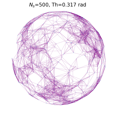
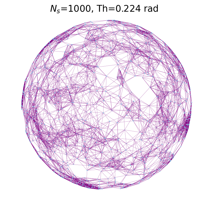
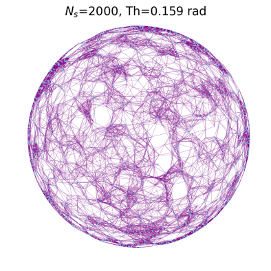
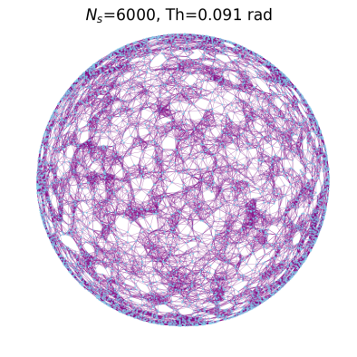
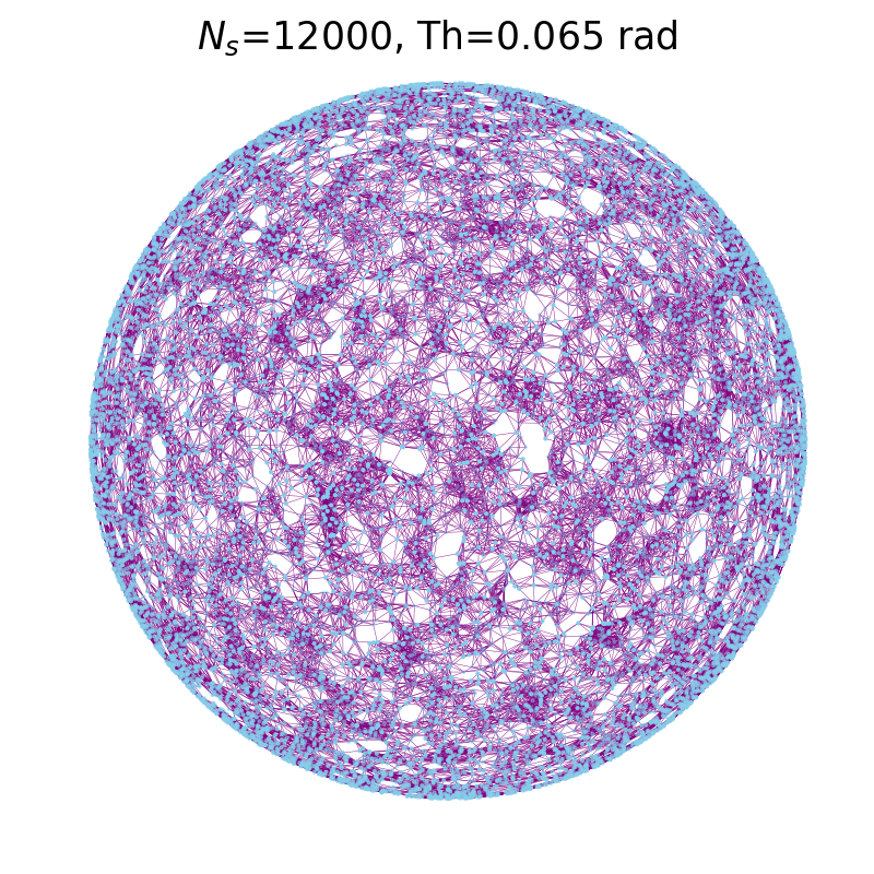
Figure 1: Illustrative graph representation for the different number of sources. The number of edges for each graph has been chosen to ensure that almost all points are connected. In this plot, the corresponding number of edges for each configuration is $n_{\text{ed},500}=3270$, $n_{\text{ed},1000}=6212$, $n_{\text{ed},2000}=12493$, $n_{\text{ed},6000}=36976$, $n_{\text{ed},12000}=75944$, respectively.

Graph Neural Network

Among all the different types of GNN tasks, graph classification is used to classify entire graphs into various categories, based on structural graph features of a given dataset of graphs. We use PyTorch Geometric [42].

Firstly, we create graphs as input for the GNN. In our graph structure each node is represented by a source position, with six features. We evaluate the Haversine distance between each pair of points and an edge between two nodes is formed if their distance is less than a given threshold. To ensure that each node is connected to its neighbors, the threshold is chosen slightly larger than the average distance. The average distance scales as $\propto N_{s}^{-1/2}$ and the distance threshold we used are $0.317$ rad, $0.224$ rad, $0.159$ rad, $0.091$ rad and $0.065$ rad for $N_{s}=500$, $N_{s}=1000$, $N_{s}=2000$, $N_{s}=6000$, and $N_{s}=12000$, respectively. In this way, we can preserve the local structural relationships necessary for accurate predictions without introducing unnecessary complexity.

To store the graph data, we use Data tool from PyTorch Geometric. It takes node features, graph connectivity, positions and labels (in this case one value of $\Omega_{\text{GW}}$ for the entire graph), and constructs the graph representation for a given dataset. The chosen numbers of sources and realizations are the same of the FCN. To illustrate what a single representation looks like, we plot the graph representation in three dimension for different number of sources in Fig. 1.

The architecture consists of five convolution layers, by using GCNConv [43] implemented in PyTorch models, followed by a final linear layer to produce a single output value for each graph. ReLU activations are applied after each graph convolution to introduce non-linearity. At the end of the forward process, a global mean pooling operation combines node embeddings into a graph-level representation, using a global mean pooling operation. Finally, a dropout layer with probability of 0.5 is added, and the linear layer outputs the final prediction. The input size corresponds to the number of features, while each hidden layer contains 128 neurons.

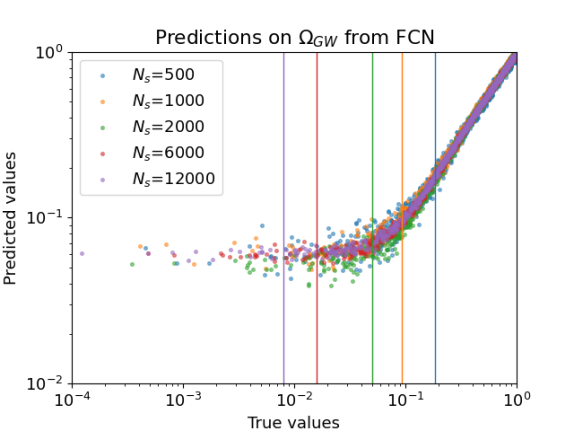
Figure 2: Predictions in logarithmic scale on $\Omega_{\text{GW}}$ values, which were uniformly distributed in the range $[0,1]$. The left panel represents the result of FCN, while the right panel the one from GNN. The vertical line is the theoretical estimate for $\Omega_{\text{GW}}$ given by Eq. (3). The predicted values are obtained using the test set ($1600$ samples, the $20\%$ of the original dataset of $8000$ mocks).

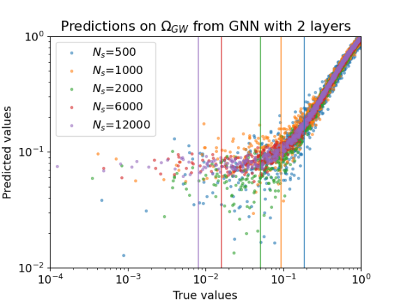
Figure 3: Comparison of GNN results for different numbers of layers. Predictions are produced in the same way as in Fig. 2, where the GNN has five layers. The left panel shows the results from a GNN with only two convolutional layers, while the right panel shows the results from a GNN with three convolutional layers in its architecture.

The training process uses Adam optimizer with learning rate of $10^{-4}$ and MSE loss function. We implement an early stopping technique, with patience of 100 epochs.

IV Results

Comparison between FCN and GNN

In Fig. 2, we present the test performance results for both FCN (left panel) and GNN (right panel). The networks can perform quite well for higher values of $\Omega_{\text{GW}}$, while the predictions start to become less precise for lower values, when the noise starts to dominate. The vertical line is the theoretically estimated sensitivity for $\Omega_{\text{GW}}$ given by Eq. (3) included for reference. Note that this theoretical estimate assumes the same proper motion errors for all sources, whereas our mock data does not satisfy this assumption, as the proper motion errors depend on the magnitude of the sources. The results do not necessarily need to completely align with the theoretical line. However, we observe a tendency for the estimated $\Omega_{\text{GW}}$ values to scatter when the true value is smaller than the theoretical line, where the data is expected to be dominated by noise. As one can notice, by increasing the number of sources, the lines moves towards left, due to the inverse proportionality to the number of objects as seen in Eq. (3) and the NN predictions also improve with an increasing number of sources.

Note that the plot is shown in log-scale, while our mock catalog dataset is generated with a linear-uniform distribution of $\Omega_{\text{GW}}$. We have tested both linear-uniform and log-uniform distribution of $\Omega_{\text{GW}}$ and found that NNs perform better with the linear-uniform distribution. Additionally, for the GNN, we evaluated the impact of varying distance threshold values used to define the graph connectivity for a fixed number of sources. We observed that variations in the distance threshold did not lead to substantial differences in the trained performance of the GNN.

The FCN exhibits a tendency to plateau in its predictive accuracy for smaller target values of $\Omega_{\text{GW}}$. This behavior suggests that the network struggles to capture distinctions in the lower value range, potentially due to its inherent limitations in representing complex relationships for this specific problem and the similarity of proper motion values and uncertainties to the level of noise in the data. The plateau indicates that the FCN saturates in its capacity to learn from the data with small $\Omega_{\text{GW}}$ values.

In contrast, the GNN demonstrates the ability to closely track the diagonal representing the ideal one-to-one correspondence between predicted and true values, across small values of $\Omega_{\text{GW}}$. These predictions exhibit a higher degree of dispersion for smaller $\Omega_{\text{GW}}$, which seems to be less accentuated for higher number of sources. This suggests that the GNN captures the overall trends effectively. Its dispersion appropriately increases for smaller $\Omega_{\text{GW}}$ values, reflecting its ability to adapt to the inherent uncertainties in the data.

These differences can be linked to the intrinsic design of each architecture. Interestingly, for GNN, modifications of the architecture play a role between model complexity and predictive behavior. In fact, when the depth of the GNN is reduced, for instance by decreasing the number of convolutional layers to two or three, the model begins to exhibit a behavior that parallels the plateau effect seen in the FCN, as shown in Fig. 3. Despite this plateau-like behavior, the characteristic scatter of GNN predictions persists, even with fewer layers. This indicates that the scatter is not only a function of model depth but might also come from intrinsic factors such as how the GNN aggregates and propagates information within the graph structure. Although deeper GNNs are better for capturing complex dependencies, they also introduce challenges such as greater variability in predictions. These observations underscore the complex relationship between model design choices and performance outcomes, resulting in careful tuning of model architectures to balance precision and stability for specific tasks.

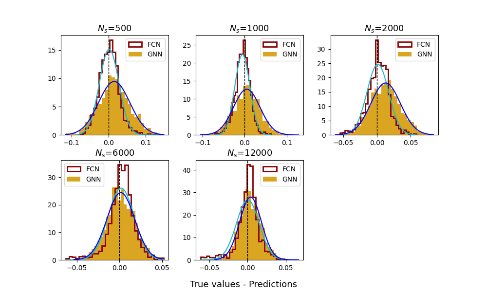
Figure 4: The probability distribution of deviations between the true and predicted values for $\Omega_{\text{GW}}$ is plotted using the results obtained from the test dataset in Fig. 2. The cyan curve represents the Gaussian fit to the FCN results, while the blue curve represents the Gaussian fit to the GNN results.

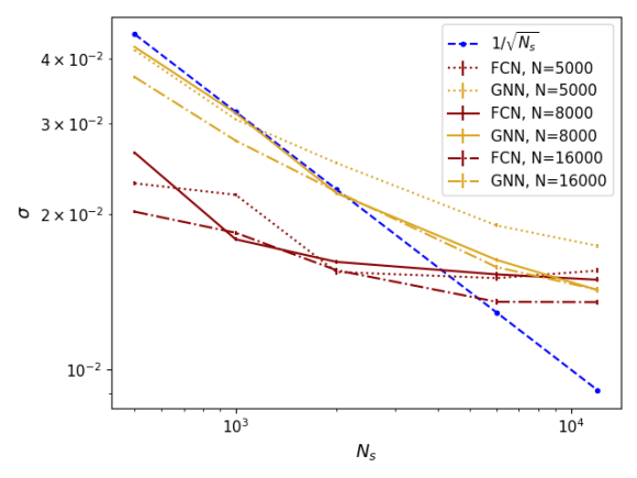
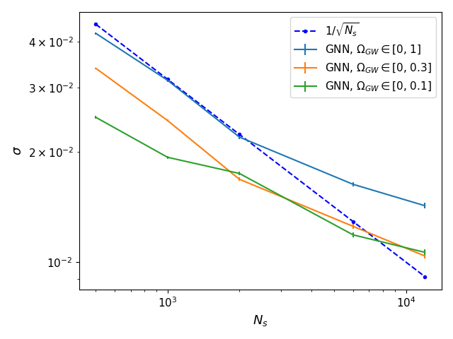
Figure 5: The variance of the residual distributions in Fig. 4 is plotted as a function of the number of sources. In the left panel, solid lines represent the results for predictions in Fig. 4 for the FCN (yellow) and GNN (brown). Other curves correspond to results obtained by varying the number of mock data. These predictions are generated using test datasets, which constitute $20\%$ of the original mock datasets. The original mock datasets consist of $5000$ (dotted lines), $8000$ (solid lines), and $16000$ (dashdot lines) samples, respectively. The blue dashed line represents the theoretical sensitivity estimate, where the statistical error decreases proportional to $1/\sqrt{N_{s}}$, with $N_{s}$ being the number of sources. In the right panel, the variance of the residual distributions is shown by varying the range of $\Omega_{\text{GW}}$ sampling. The default range of $[0,1]$ is reduced to $[0,0.3]$ and further to $[0,0.1]$. The number of mock datasets is fixed at $8000$. Results are displayed only for the GNN.

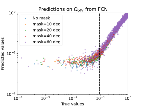
Figure 6: Predicted values of $\Omega_{\text{GW}}$ for the masked dataset are tested by changing the area of the mask. The number of sources is fixed to $N_{s}=1000$. The left panel represents the result of FCN, while the right panel the one from the GNN.

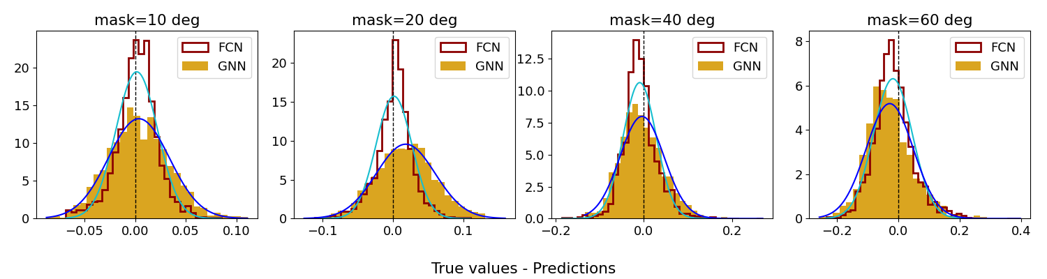
Figure 7: The probability distributions of deviations between the true and predicted values for $\Omega_{\text{GW}}$ is plotted using the results obtained from the test dataset in Fig. 6, in the case of masked datasets. The cyan curve represents the Gaussian fit to the FCN results, while the blue curve represents the Gaussian fit to the GNN results.

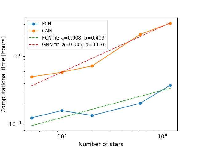
Figure 8: Plot of the computational time in a logarithmic scale. The dashed lines correspond to a power-law fit of the form $y(x)=a\cdot x^{b}$. The best-fit values for $a$ and $b$ are shown in the legend.

Distributions of the variance and its dependence on the source number

To further analyze the performance of the models, we plot in Fig. 4 the distribution of the residuals, i.e., the difference between the predicted and true values. We observe that the variance of the FCN is generally smaller than that of the GNN. However, the residual distribution of the FCN is more non-Gaussian and exhibits larger tails, corresponding to small $\Omega_{\text{GW}}$ realizations where the FCN displays plateau behavior in Fig. 2. For reference, we also include the Gaussian fit of the histogram in the plot.

Furthermore, we observe a clear trend where the width of the distribution decreases as the number of sources increases. To investigate this trend more explicitly, Fig.5 shows the variance as a function of the number of sources $N_{s}$. The non-smooth behavior of the curves is due to statistical fluctuations. We tested that by performing at least three runs for each point, the average profile of the trend becomes smoother, but the overall trend remains the same. For reference, we also plot a line proportional to $N_{s}^{-1/2}$, which corresponds to the theoretical prediction for astrometric sensitivity, as indicated in Eq.(3).

The left panel compares the FCN and GNN results. Consistent with Fig. 4, the FCN exhibits a smaller variance compared to the GNN. However, the variance does not decrease as $1/\sqrt{N_{s}}$ for larger numbers of sources, potentially highlighting limitations of the architecture. For the GNN, this sensitivity saturation is less pronounced but still deviates from the $1/\sqrt{N_{s}}$ scaling for large $N_{s}$. To investigate this further, we conduct additional tests by varying the number of mock data $N$, plotted in the same figure, based on the hypothesis that the requirement for more catalog realizations becomes increasingly critical as $N_{s}$ grows. We observe that the result is indeed affected when comparing the lines for $N=5000$ and $N=8000$. However, we do not find any significant difference between $N=8000$ and $N=16000$, indicating that the original number of mocks used ($N=8000$) is sufficient for our configurations.

In the right panel, we test another hypothesis that the range of $\Omega_{\text{GW}}$ for the mock data should be optimized based on the sensitivity. The theoretical sensitivity is $\Omega_{\text{GW}}\sim 0.2$ for $N_{s}=500$, while $\Omega_{\text{GW}}\sim 0.08$ for $N_{s}=12000$, but both are trained using the same range of $\Omega_{\text{GW}}=[0,1]$. As one may notice in Fig. 2, the NNs do not have many samples for noise-dominated data in the case of $N_{s}=12000$, which may explain the reduction in sensitivity. To investigate this, we test two different ranges for $\Omega_{\text{GW}}$: $\Omega_{\text{GW}}=[0,0.3]$ and $\Omega_{\text{GW}}=[0,0.1]$. We observe an improvement in sensitivity, and the $N_{s}=12000$ data point gets closer to the $1/\sqrt{N_{s}}$ curve. However, we also notice that the variance for $N_{s}=500$ decreases, likely because the samples are now taken only from small $\Omega_{\text{GW}}$ cases. While it is difficult to draw a firm conclusion from this test, it highlights the importance of the training range, as it is analogous to setting prior knowledge for the parameter values to be predicted.

Inhomogeneous case: masked samples

In the above, we have demonstrated the application of NNs with simplified mock data settings. However, there are many complex factors to consider when handling real data, and this presents a much longer path to fully realizing the potential of NNs. We leave it for the future work, while here, to illustrate one example of the flexibility of NNs, we apply them to masked data and evaluate their performance.

We fix the number of sources to $N_{s}=1000$ and mask the regions of the data set corresponding to the declination of $\delta=10^{\circ}$, $20^{\circ}$, $40^{\circ}$, and $60^{\circ}$. While we are aware that $\delta=60^{\circ}$ is non-realistic value for the mask, it is used here solely for training performance purposes. The same NN architectures are trained on these masked subsets and the results are shown in Figs. 6 and 7.

Despite the variation in input data coverage, the general trends in the results remain consistent: the FCN exhibits a plateau in performance for smaller target values, while the GNN maintains its characteristic diagonal alignment with the true values, as seen in Fig.6. The NNs successfully predict the values of $\Omega_{\rm GW}$ when the signal is dominant, but an increased dispersion is now present in the predictions of both networks, which is more clearly observed in the distributions reported in Fig.7. As expected, we observe that the variance increases with a larger mask area. This results suggests that NNs are capable of performing reasonably well even when the source distribution is inhomogeneous.

Computation time

Given the expected number of sources available in future data, a reduction in computation time is primarily anticipated for the NNs. To address this, the computational time (including the training time) is plotted in Fig. 8. All these results were evaluated on a GPU cluster. As observed, in both cases, the computation time increases logarithmically with the number of sources. The GNN exhibits higher steep in terms of time, which highlights the higher computational complexity inherent to the network itself and the manage of more complex data in input. In both cases, the behavior reflects a more accentuate computational cost for larger datasets.

Both networks are competitive in predicting the value of $\Omega_{\text{GW}}$, with some differences in the noise-dominated regime, while the FCN shows an advantage in terms of the computation time. This is probably because the architecture of the FCN is simpler compared to that of the GNN, and the GNN requires handling graph structures, which can be more complex for simple mock datasets. This complexity makes the implementation and computation less efficient and less competitive.

V Conclusions

In this work, we have explored the possibility of constraining SGWB through astrometric measurements, with a particular focus on the application of NNs. These networks could provide complementary tools to traditional methods for detecting and constraining the SGWB, which is an interesting possibility, especially in the context of current or upcoming surveys that could uncover new aspects of the cosmological history of the Universe.

Specifically, we analyze the performance of two NN architectures, an FCN and a GNN on a regression task to predict the value of the SGWB amplitude $\Omega_{\text{GW}}$. The results highlight distinct strengths and limitations for each architecture. The FCN consistently exhibits a plateau effect for small values across all tests, indicating its limitations in capturing the correct relationships in this range. This plateau persists even when the number of sources is varied or the datasets are masked. This behavior can be interpreted as a sign of reduced accuracy, particularly for small values of $\Omega_{\text{GW}}$. In contrast, the GNN tracks the ideal diagonal in the predictions with increasing dispersion for smaller $\Omega_{\text{GW}}$.

The GNN exhibits more stable behavior in terms of extracting the value of $\Omega_{\text{GW}}$, as the distribution of the predictions is closer to Gaussian, and the sensitivity scales with the theoretically predicted trend $\propto N_{s}$, with some exceptions for the large $N_{s}$ case. On the other hand, the FCN, while showing good sensitivity overall, saturates for specific configurations, but it demonstrates a significant advantage in terms of computation time. Our results suggest that the choice of architecture should be guided by the specific requirements of the task, balancing accuracy, stability, and computational efficiency.

NNs will become essential tools for analyzing the large volumes of upcoming astrometric data with accounting for systematic uncertainties. This paper provides the first step toward the new application of NNs to GW astrometry. In particular, the GNN implementation is a relatively unexplored field, and we expect that its advantages will become more pronounced when dealing with more complicated models of the dataset, particularly when applying the analysis to real data. While there are still challenges to be addressed, the promising results from this work highlight the potential of NNs in advancing GW astrometry.

References

- Starobinsky [1979] A. A. Starobinsky, JETP Lett. 30, 682 (1979).
- Damour and Vilenkin [2000] T. Damour and A. Vilenkin, Phys. Rev. Lett. 85, 3761 (2000), arXiv:gr-qc/0004075 .
- Kosowsky et al. [1992] A. Kosowsky, M. S. Turner, and R. Watkins, Phys. Rev. D 45, 4514 (1992).
- Regimbau [2011] T. Regimbau, Res. Astron. Astrophys. 11, 369 (2011), arXiv:1101.2762 [astro-ph.CO] .
- Caprini and Figueroa [2018] C. Caprini and D. G. Figueroa, Class. Quant. Grav. 35, 163001 (2018), arXiv:1801.04268 [astro-ph.CO] .
- Kuroyanagi et al. [2018] S. Kuroyanagi, T. Chiba, and T. Takahashi, JCAP 11, 038, arXiv:1807.00786 [astro-ph.CO] .
- Christensen [2018] N. Christensen, Reports on Progress in Physics 82, 016903 (2018).
- Colpi et al. [2024] M. Colpi et al., (2024), arXiv:2402.07571 [astro-ph.CO] .
- Kawamura et al. [2021] S. Kawamura et al., PTEP 2021, 05A105 (2021), arXiv:2006.13545 [gr-qc] .
- Abbott et al. [2017] B. P. Abbott, R. Abbott, T. D. Abbott, M. R. Abernathy, K. Ackley, C. Adams, P. Addesso, R. X. Adhikari, and at al, Classical and Quantum Gravity 34, 044001 (2017).
- Domcke [2023] V. Domcke, in 57th Rencontres de Moriond on Electroweak Interactions and Unified Theories (2023) arXiv:2306.04496 [gr-qc] .
- Hazumi et al. [2020] M. Hazumi et al. (LiteBIRD), Proc. SPIE Int. Soc. Opt. Eng. 11443, 114432F (2020), arXiv:2101.12449 [astro-ph.IM] .
- Agazie et al. [2024] G. Agazie et al. (International Pulsar Timing Array), Astrophys. J. 966, 105 (2024), arXiv:2309.00693 [astro-ph.HE] .
- Pyne et al. [1996] T. Pyne, C. R. Gwinn, M. Birkinshaw, T. M. Eubanks, and D. N. Matsakis, Astrophys. J. 465, 566 (1996), arXiv:astro-ph/9507030 .
- Jaffe [2004] A. H. Jaffe, New Astron. Rev. 48, 1483 (2004), arXiv:astro-ph/0409637 .
- Book and Flanagan [2011] L. G. Book and E. E. Flanagan, Phys. Rev. D 83, 024024 (2011).
- Mihaylov et al. [2018] D. P. Mihaylov, C. J. Moore, J. R. Gair, A. Lasenby, and G. Gilmore, Phys. Rev. D 97, 124058 (2018), arXiv:1804.00660 [gr-qc] .
- Mihaylov et al. [2020] D. P. Mihaylov, C. J. Moore, J. Gair, A. Lasenby, and G. Gilmore, Phys. Rev. D 101, 024038 (2020), arXiv:1911.10356 [gr-qc] .
- Prusti et al. [2016] T. Prusti et al. (Gaia), Astron. Astrophys. 595, A1 (2016), arXiv:1609.04153 [astro-ph.IM] .
- Gwinn et al. [1997] C. R. Gwinn, T. M. Eubanks, T. Pyne, M. Birkinshaw, and D. N. Matsakis, Astrophys. J. 485, 87 (1997), arXiv:astro-ph/9610086 .
- Titov et al. [2011] O. Titov, S. B. Lambert, and A. M. Gontier, Astron. Astrophys. 529, A91 (2011), arXiv:1009.3698 [astro-ph.CO] .
- Darling et al. [2018] J. Darling, A. E. Truebenbach, and J. Paine, The Astrophysical Journal 861, 113 (2018).
- Jaraba et al. [2023] S. Jaraba, J. García-Bellido, S. Kuroyanagi, S. Ferraiuolo, and M. Braglia, Mon. Not. Roy. Astron. Soc. 524, 3609 (2023), arXiv:2304.06350 [astro-ph.CO] .
- Darling [2024] J. Darling, (2024), arXiv:2412.08605 [astro-ph.CO] .
- Yeh et al. [2022] T.-H. Yeh, J. Shelton, K. A. Olive, and B. D. Fields, JCAP 10, 046, arXiv:2207.13133 [astro-ph.CO] .
- Kite et al. [2021] T. Kite, A. Ravenni, S. P. Patil, and J. Chluba, Mon. Not. Roy. Astron. Soc. 505, 4396 (2021), arXiv:2010.00040 [astro-ph.CO] .
- Wang et al. [2022] Y. Wang, K. Pardo, T.-C. Chang, and O. Doré, Phys. Rev. D 106, 084006 (2022), arXiv:2205.07962 [gr-qc] .
- Pardo et al. [2023] K. Pardo, T.-C. Chang, O. Doré, and Y. Wang, (2023), arXiv:2306.14968 [astro-ph.GA] .
- Malbet et al. [2022] F. Malbet et al., in SPIE Astronomical Telescopes + Instrumentation 2022 (2022) arXiv:2207.12540 [astro-ph.IM] .
- García-Bellido et al. [2021] J. García-Bellido, H. Murayama, and G. White, JCAP 12 (12), 023, arXiv:2104.04778 [hep-ph] .
- Moore et al. [2017] C. J. Moore, D. P. Mihaylov, A. Lasenby, and G. Gilmore, Phys. Rev. Lett. 119, 261102 (2017), arXiv:1707.06239 [astro-ph.IM] .
- Maggiore [2007] M. Maggiore, Gravitational Waves. Vol. 1: Theory and Experiments (Oxford University Press, 2007).
- Romano and Cornish [2017] J. D. Romano and N. J. Cornish, Living Rev. Rel. 20, 2 (2017), arXiv:1608.06889 [gr-qc] .
- [34] https://github.com/agabrown/PyGaia.
- Storey-Fisher et al. [2024] K. Storey-Fisher, D. W. Hogg, H.-W. Rix, A.-C. Eilers, G. Fabbian, M. R. Blanton, and D. Alonso, Astrophys. J. 964, 69 (2024), arXiv:2306.17749 [astro-ph.GA] .
- [36] https://www.cosmos.esa.int/web/gaia/science-performance.
- Mignard and Klioner [2012] F. Mignard and S. Klioner, Astron. Astrophys. 547, A59 (2012), arXiv:1207.0025 [astro-ph.IM] .
- Zhou et al. [2020] J. Zhou, G. Cui, S. Hu, Z. Zhang, C. Yang, Z. Liu, L. Wang, C. Li, and M. Sun, AI Open 1, 57 (2020).
- Sanchez-Lengeling et al. [2021] B. Sanchez-Lengeling, E. Reif, A. Pearce, and A. B. Wiltschko, Distill 10.23915/distill.00033 (2021), https://distill.pub/2021/gnn-intro.
- Agarap [2019] A. F. Agarap, Deep learning using rectified linear units (relu) (2019), arXiv:1803.08375 [cs.NE] .
- Kingma and Ba [2017] D. P. Kingma and J. Ba, Adam: A method for stochastic optimization (2017), arXiv:1412.6980 [cs.LG] .
- Fey and Lenssen [2019] M. Fey and J. E. Lenssen, Fast graph representation learning with pytorch geometric (2019), arXiv:1903.02428 [cs.LG] .
- Kipf and Welling [2017] T. N. Kipf and M. Welling, Semi-supervised classification with graph convolutional networks (2017), arXiv:1609.02907 [cs.LG] .