Impact of reionization history on constraining primordial gravitational waves in future all-sky cosmic microwave background experiments
Abstract
We explore the impact of the reionization history on examining the shape of the power spectrum of the primordial gravitational waves (PGWs) with the cosmic microwave background (CMB) polarization. The large-scale CMB generated from the reionization epoch is important in probing the PGWs from all-sky experiments, such as LiteBIRD. The reionization model has been constrained by several astrophysical observations. However, its uncertainty could impact constraining models of the PGWs if we use large-scale CMB polarization. Here, by expanding the analysis of Mortonson & Hu (2007), we estimate how reionization uncertainty impacts constraints on a generic primordial tensor power spectrum. We assume that CMB polarization is measured by a LiteBIRD-like experiment and the tanh model is adopted for a theoretical template when we fit data. We show that constraints are almost unchanged even if the true reionization history is described by an exponential model, where all parameters are within 68% Confidence Level (CL). We also show an example of the reionization history that the constraints on the PGWs are biased more than 68% CL. Even in that case, using -mode power spectrum on large scales would exclude such a scenario and make the PGW constraints robust against the reionization uncertainties.
I Introduction
Measurements of the cosmic microwave background (CMB) anisotropies have extensively explored the origin of the universe. For example, observed CMB angular power spectra are in excellent agreement with the prediction of the Cold-Dark-Matter (CDM) model. In the standard cosmological scenario, cosmic inflation, a period of rapid quasi-exponential expansion in the early universe brout1978creation ; kazanas1980dynamics ; starobinsky1980new ; guth1981inflationary ; sato1981first ; albrecht1982cosmology ; linde1982new , generates primordial density fluctuations through quantum fluctuations in the space-time metric mukhanov1981quantum ; guth1982fluctuations ; hawking1982development ; linde1982scalar ; starobinsky1982dynamics ; bardeen1983spontaneous , which will eventually become the structure of the universe. While the predicted primordial density fluctuations have already been tested by various astrophysical observations, the gravitational waves produced in the very early universe (primordial gravitational waves, PGWs) starobinskii1979spectrum ; rubakov1982graviton ; fabbri1983effect ; abbott1984constraints predicted by cosmic inflation remain unconfirmed.
The most effective method for detecting PGWs is through the curl pattern (-modes) in CMB polarization maps, as linear-order density fluctuations do not generate -modes but are sensitive to PGWs kamionkowski1997probe ; kamionkowski1997statistics ; seljak1997measuring ; seljak1997signature ; zaldarriaga1997all . The amplitude of the tensor power spectrum parameterized by the tensor-to-scalar ratio, , provides insights into the energy scale of inflation davis1992cosmic ; kamionkowski2016quest ; achucarro2022inflation ; ade2021improved . Current CMB observations set upper limits on PGWs, refining inflationary models, with the best constraints from combined BICEP/Keck Array, Planck, and WMAP data, yielding at the pivot scale Mpc-1 at 95% Confidence Level (CL) Tristram:2022 . Currently, the Simons Observatory is observing the -mode polarization precisely to reduce CL uncertainties of to Namikawa:2021gyh ; SimonsObservatory:2024:r . In the 2030s, LiteBIRD, a satellite designed for full-sky observations, aims at achieving the uncertainty to below litebird2023probing ; LiteBIRD:2023:delens . If current and future CMB experiments can yield an upper limit at , it will constrain any single-field model with a characteristic potential scale larger than the Planck scale litebird2023probing .
Next-generation CMB experiments aim to detect PGWs predicted by many inflationary models through large-scale -mode signals, particularly at the reionization bump. This bump is shaped by Thomson scattering with free electrons during the reionization epoch, where neutral hydrogen was ionized by energetic photons from early luminous sources (see e.g. Natarajan:2014rra for a review). The amplitude and the exact shape of the bump are affected by the poorly constrained reionization history, making it crucial to address uncertainties from reionization history in PGW detection.
CMB measurements have offered insights into the reionization epoch Lewis:2006ym ; WMAP7 ; Planck:2016mks ; Heinrich:2016ojb ; Hazra:2018eib ; Millea:2018bko ; Ahn:2020btj ; Qin:2020xrg . For example, Planck 2018 data constrains the optical depth to the CMB to ( CL), corresponding to a reionization redshift ( CL) aghanim2020planck . This constraint is very close to that obtained recently with the Planck Public Release 4 Tristram:2023:PR4 . However, if we only use small-scale CMB measurements to avoid the uncertainties in the large-scale -modes, recent constraints suggest ( CL) giare2024measuring , indicating challenges in precision. High-redshift quasar and galaxy observations provide additional constraints. Gunn-Peterson troughs gunn1965density suggest reionization completed by fan2006survey , while Lyman- optical depth fluctuations in quasar spectra bosman2022hydrogen and the inferred low mean free path of ionizing photons gaikwad2023measuring indicate a later completion around .
Measurements of the reionization history are even less precise, particularly regarding the time and spatial variations at higher redshifts Dai:2018nce . The Ly emission line, sensitive to neutral hydrogen, is a crucial probe ouchi2020observations , but Ly emitters (LAEs) at high redshifts () are exceedingly rare, making it challenging to use these emitters to constrain the reionization history nakane2024lyalpha . In contrast, reconstructing reionization history with CMB needs an accurate polarization observation at large-angular scales to precisely measure the reionization bump Hu:2003gh ; Hazra:2018eib ; Watts:2020 ; Sakamoto:2022nth . These limitations leave a wide range of models viable under current constraints, highlighting significant uncertainties in our understanding of reionization. The uncertainties from the reionization history might affect the accuracy of reconstructing PGWs from polarization signals Mortonson:2007tb ; Lau:2013zea . Uncertainties in the reionization history could also impact the constraints on cosmology models beyond CDM Paoletti:2020ndu and on the kinetic Sunayev Zel’dovich effect from reionization Gorce:2022cvb .
Mortonson & Hu (2007) Mortonson:2007tb explore the impact of the reionization history on the constraints on , assuming Planck or CMBPol experiment, as well as cosmic-variance limited cases. They assume or as a fiducial parameter, both of which are almost excluded by the current -mode measurements, so it is important to study again for consistent with the current observation. Lau et al. (2013) Lau:2013zea investigated this problem in partial sky assuming Planck case. Several works have also studied the impacts of patchy reionization on the constraints on jain2023framework ; mukherjee2019patchy ; jain2024disentangling .
The present paper builds upon previous studies in two significant ways. First, we examine how uncertainties in the reionization history affect constraints on a generic primordial tensor power spectrum (PTPS). Previous studies typically assumed a standard scale-invariant spectrum for PTPS. However, full-sky CMB experiments, such as those targeting the -mode signal, allow us to constrain the deviation of the tensor power spectrum from the standard PTPS parameterized by . By measuring the -mode power spectrum at both the reionization and recombination bumps, we can differentiate between various models of PGWs, such as the SU(2)-axion model LiteBIRD:2023zmo , and explore more general forms of the PTPS hiramatsu2018reconstruction . Second, we improve upon the experimental assumptions of previous studies. Earlier works considered CMB experimental configurations with significantly higher polarization noise than what is expected from upcoming missions or a cosmic-variance-limited scenario, making those assumptions unrealistic. In the near future, LiteBIRD will achieve a polarization noise level of approximately K-arcmin by combining all frequency channels. LiteBIRD is highly sensitive to , with a projected 68% CL uncertainty of litebird2023probing . Under such precise measurements, the impact of reionization history on constraints becomes more critical than in previous experiments.
This paper is organized as follows. In Sec. II, we describe the PTPS and reionization history we consider in this paper. In Sec. III, we explain our forecast setup and how we derive parameter constraints. In Sec. IV, we show how the uncertainties in the reionization model impact the constraint on the PTPS. Sec. V is devoted to summary and discussion.
Throughout this paper, we assume the flat CDM model as our fiducial model. We assume that the Hubble parameter is km/s/Mpc and define as the Hubble parameter divided by km/s/Mpc. We also assume the physical baryon energy density, , physical CDM energy density, , spectral index of the scalar primordial power spectrum, , and its amplitude, . These values are consistent with the results from the Planck collaboration aghanim2020planck .
II Models
In this section, we describe the PTPS and reionization models considered in this paper. We modify the public code, CLASS, (blas2011cosmic, ), to compute the CMB polarization angular power spectra with these models.
II.1 The primordial tensor power spectrum
We generalize the standard scale-invariant spectrum by following the steps outlined in Hiramatsu et al. (2018) hiramatsu2018reconstruction . Specifically, we characterize the deviation of the PTPS from the standard case as
| (1) |
where represents the dimensionless amplitude of the PTPS with being constants. Here, is the number of bins in logarithmic intervals. The values of are given by , where controls the logarithmic interval. We set Mpc-1, and , same as the set in Hiramatsu et al. (2018) hiramatsu2018reconstruction . In this paper, we assume
| (2) |
where is the amplitude of the PTPS, is the tensor spectral index, and is the running of the tensor spectral index. The amplitude is given by defined at the pivot scale, , where is the amplitude of the curvature perturbations and is the tensor-to-scalar ratio. We assume that and follow the slow-roll inflationary consistency relation as lidsey1997reconstructing :
| (3) |
where is the scalar spectral index. The PTPS at low- and high-, could be modified in the SU(2)-axion model, while the spectrum is enhanced at intermediate scales by the massive gravity inflation model predicts hiramatsu2018reconstruction .
II.2 Reionization models
We first introduce the hyperbolic tangent (tanh) model that has been widely used in constraining cosmological parameters with CMB angular power spectra. In this model, the reionization history is divided into two phases: the phase before reionization begins (), where the free-electron fraction remains constant at , and reionization epoch (), during which evolves as
| (4) |
where we define
| (5) |
Here, is the redshift when and is the duration of the reionization epoch. We fix and vary in our forecast. The free-electron fraction before the reionization, , and the contributions from Helium, , are derived from the HyRec code implemented in CLASS. The starting redshift of reionization, , is given by .
From the reionization history, , we often compute the optical depth to the CMB defined as
| (6) |
where is the scale factor, is proton number density, is the Thomson scattering cross-section, and with the dot denoting the time derivative. We compute the proton number density as where is the critical density, is proton mass.
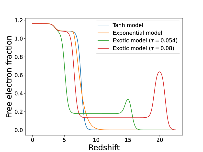
In our forecast, we consider two different models for the “true” reionization history as described in detail in the following subsection and use the tanh model for the theoretical template to fit. Figure 1 summarizes the reionization history we used in our forecast study.
II.2.1 Exponential model
The first model we consider is the exponential model described in the CAMB package (lewis2000efficient, ) where in Eq. (4) is replaced to 111The definition can be found from the source code of the CAMB package: https://github.com/cmbant/CAMB/blob/master/fortran/reionization.f90 (line 380-403).
| (7) |
Here, the evolution rate in the exponential, , is defined as
| (8) |
For simplicity, we assume that the redshift when the reionization is completed, , is fixed to . We set , which corresponds to .
II.2.2 Exotic reionization model
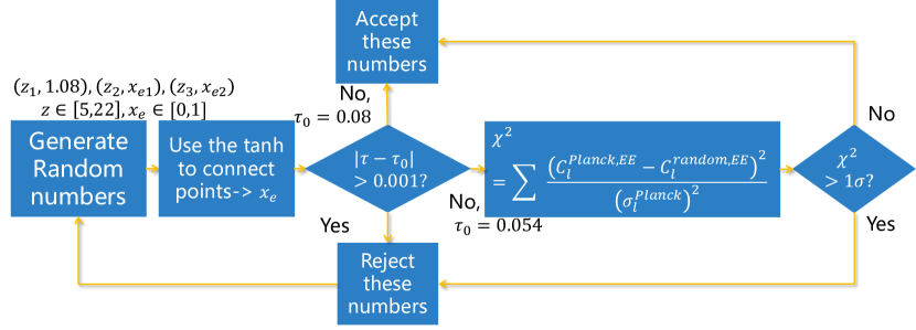
TThe other model we consider for the true reionization history is an exotic model. It demonstrates how the PTPS constraint depends on the assumed reionization history. We generate the parametrized reionization history as a function of using random points. The process is shown in Fig. 2. Note that we generate many exotic models, but this paper only shows the forecast results for a model that introduces the most significant bias among them.
In the process of generating random models, we generate three random redshift points within the range . Among these, marks the end of reionization, where , corresponding to helium reionization. We also generate two random numbers, and , between 0 and 1. A tanh function is used to connect these points. We then obtain from this reionization history and reject the model if where is either or motivated by the recent observations of Ref. tristram2023cosmological and giare2024measuring , respectively. For , we reject models which deviate significantly from the large-scale Planck -mode power spectrum. Specifically, we compute where is the Planck PR4 -mode power spectrum, is the -mode power spectrum with a generated , and is the measurement error of Planck PR4 data taken from Ref. tristram2023cosmological . For , we do not consider further rejections since is obtained without relying on the large-scale Planck -mode power spectrum giare2024measuring . After randomly generating models, we choose a case where the reionization history significantly deviates from the tanh case. We generate the models for and respectively. The selected reionization history exhibits behavior similar to the double reionization model cen2003universe .
III Method
Here, we describe our method for the forecast study. We jointly constrain the reionization history and PTPS with the - and -mode power spectra with a Markov Chain Monte Carlo (MCMC) analysis kosowsky2002efficient . Our assumptions on the CMB experimental configurations and likelihood are described as follows.
We adopt a LiteBIRD-like CMB experiment, assuming that the observed polarization data has white noise and is convolved with a Gaussian circular beam for simplicity. The noise power spectrum for the beam-deconvolved CMB polarization map is given by (e.g. Ref. namikawa2010probing )
| (9) |
where K is the CMB black-body temperature, is the Full Width at Half Maximum (FWHM) of the circular beam in arcmin, and is the noise level of the polarization map in K-arcmin. For LiteBIRD, we assume arcmin and K-arcmin hiramatsu2018reconstruction ; LiteBIRD:2023zmo .
The likelihood for the - and -mode power spectra in an idealistic full-sky observation are given as a Wishart distribution Hamimeche:2008ai . Specifically, we employ the following log-likelihood function katayama2011simple ; litebird2023probing :
| (10) |
Here, represents mock data and is computed either with the exponential or exotic reionization history. The theoretical power spectra, , are defined using the tanh function to describe the reionization history, and the vector refers to the set of free parameters. The polarization noise power spectrum is denoted by . The minimum and maximum multipoles of the power spectra are and , respectively, where is set to . For the maximum multipole, we choose for the -mode power spectrum and for the -mode power spectrum. Our results are not sensitive to the maximum multipole of the -mode power spectrum as long as we set where the PGW contributions are not important. Finally, is the sky coverage, for which we set , and we follow Ref. LiteBIRD:2023zmo where the entire log-likelihood is scaled by .
We consider , ’s, and the optical depth to the CMB, , as the free parameters. 222In our calculation, we vary in the tanh model. Since we fix , we obtain from . Since the small-scale -mode power spectrum, given by , is well constrained by the temperature power spectrum, we fix by adjusting to keep it unchanged Mortonson:2007tb . For the fiducial parameters, we test two cases: and , while setting . For the optical depth, we consider that matches the latest result from the Planck collaboration aghanim2020planck , and obtained without relying on the large-scale -mode measurement giare2024measuring . 22footnotetext: https://wiki.cosmos.esa.int/planck-legacy-archive/images/b/be/Baseline_params_table_2018_68pc.pdf We modify emcee foreman2013emcee to perform the MCMC analysis. We also modify CLASS lewis2000efficient to compute the power spectra with the reionization histories and PTPS described above.
IV Results
In this section, we show the results of our forecast. We use the tanh model to fit the mock power spectra in which the exponential or exotic models are used for the reionization history.
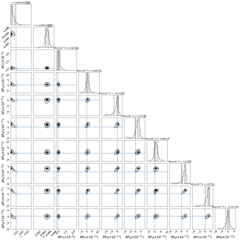
Figure 3 shows the results of the MCMC analysis where the fiducial model is the exponential model with , , and . The fiducial values are within the confidence contours, showing that the incorrect tanh reionization model did not result in a significant bias to the constraints on the PTPS. Note that we also change the optical depth to and the tensor-to-scalar ratio to , but find that the parameters are also within 68% confidence contours. The constraint at CL is approximately consistent with that obtained in Ref. hiramatsu2018reconstruction , although there are several differences in the forecast setup. We find that ’s except for show a positive degeneracy. Conversely, shows negative degeneracy with other than . This behavior is attributed to the fact that an increase (decrease) of is compensated by decreasing (increasing) with . In contrast, if increases, the -mode power spectrum at is enhanced while is enhanced slightly, leading to a scale-dependent change in the power spectrum. The optical depth is almost not degenerated with other parameters as the reionization history would be tightly constrained by the reionization bump in the -mode power spectrum.
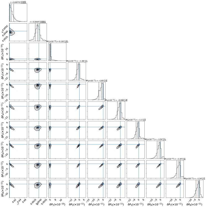
Figure 4 shows the results of the parameter constraints for the exotic model whose reionization history, , is shown as the red line in Fig. 1. The fiducial values of the parameters are , , and . The results show that the best-fit values are biased by more than , especially for the tensor-to-scalar ratio, optical depth, and . The bias to the small-scale tensor amplitudes, and , is the result of the change in the -mode power spectrum at high- by the exotic model; the high ionization fraction at high redshift amplifies the polarization power spectra at multipoles larger than the reionization bump Hu:2003gh . At , this amplification affects both the - and -mode power spectra at higher multipoles, i.e., , than the reionization bump. To fit the amplified reionization bump in the -mode power spectrum, the best-fit becomes very small, leading to a significant bias in the value of .
Figures 5 and 6 show the corresponding - and -mode power spectra with the best-fit values for the exponential and exotic models, respectively, and compare them with the fiducial power spectra with the observational errors at CL at each multipole for the LiteBIRD-like experiment. The observational errors at each multipole on the - and -mode power spectra are given by (e.g., Ref. namikawa2010probing ):
| (11) |
For the exponential model, both the best-fit - and -mode power spectra show excellent agreement with the fiducial spectrum. However, for the exotic model, while the -mode power spectrum can be fitted well, the best-fit -mode power spectrum is far from the fiducial power spectrum, especially for the reionization bump. This discrepancy in the -mode power spectrum leads to a significant bias in shown in Fig. 4.
V Summary and Discussion
We explored how an incorrect model of the reionization history impacts the constraints on the PTPS for the LiteBIRD-like experiment. In the exponential model case, we found that the mock - and -mode power spectra agree well with that using the best-fit parameters within the observational errors. In the exotic scenario, we showed that and at small scales are biased. However, the -mode power spectrum is not in good agreement with that computed with the best-fit values and such a scenario would be easily excluded by measuring the large-scale -mode power spectrum. Our results show that incorrect reionization models can introduce significant bias in the constraints on the tensor primordial power spectrum. To avoid potential bias from incorrect modeling of the reionization history, in future CMB experiments, it is crucial to accurately measure the -mode power spectrum to robustly constrain the PTPS.
We note that our analysis used several simplifications that do not include any practical issues in measuring the large-scale polarization power spectra. For example, the large-scale polarization is dominated by the Galactic foregrounds. Multiple works have developed foreground-cleaning methods to suppress a bias from the Galactic foregrounds in the -mode power spectrum (e.g. Refs. Stompor:2008:FGbuster ; katayama2011simple ; Ichiki:2018:delta-map ; Remazeilles:2020:cMILC ; Carones:2022:FG ). Compared to the -mode power spectrum, however, the -mode power spectrum has a large signal, and the bias from foreground residuals would be much smaller than that in the -mode power spectrum. The large-scale multipoles could also be contaminated by noise, although its impact on polarization is much less significant than in temperature. The likelihood approximation given in Eq. (10) which has been used for multiple forecast studies is not valid if we work on real cut-sky data that removed the Galactic plane and point-source contributions. Instead of introducing the scaling factor, , we should use the likelihood approximation proposed by Ref. Hamimeche:2008ai or the exact but computationally-intensive pixel-based likelihood Planck:2015 ; Gerbino:2019:likelihood . We did not consider the -mode delensing in our forecast. The delensing improves the constraint on by approximately in the Simons Observatory as the constraint on is determined by the recombination bump in the -mode power spectrum SimonsObservatory:2024:r . For LiteBIRD, the delensing improves the constraint by approximately which is mostly attributed to a reduction of the statistical errors at the recombination bump Namikawa:2021gyh . We expect that the delensing does not significantly impact our results as the reionization history modifies mostly the reionization bump. A study on these practical issues is beyond our scope and is left for our future work.
Acknowledgements.
We thank Gill Holder and Naoki Yoshida for the useful discussion and helpful comments. TN also thanks Antony Lewis for initiating this project. HJ is supported by the International Graduate Program for Excellence in Earth-Space Science (IGPEES). TN is supported in part by JSPS KAKENHI Grant No. JP20H05859 and No. JP22K03682. The Kavli IPMU is supported by the World Premier International Research Center Initiative (WPI Initiative), MEXT, Japan.References
- (1) R. Brout, F. Englert, and E. Gunzig Annals of Physics 115 (1978), no. 1 78–106.
- (2) D. Kazanas Astrophysical Journal, Part 2-Letters to the Editor 241 (1980) L59–L63.
- (3) A. A. Starobinsky Phys. Lett. B 91 (1980), no. 1 99–102.
- (4) A. H. Guth Phys. Rev. D 23 (1981), no. 2 347.
- (5) K. Sato Mon. Not. R. Astron. Soc. 195 (1981), no. 3 467–479.
- (6) A. Albrecht and P. J. Steinhardt Phys. Rev. Lett. 48 (1982), no. 17 1220.
- (7) A. D. Linde Phys. Lett. B 108 (1982), no. 6 389–393.
- (8) V. F. Mukhanov and G. Chibisov ZhETF Pisma Redaktsiiu 33 (1981) 549–553.
- (9) A. H. Guth and S.-Y. Pi Phys. Rev. Lett. 49 (1982), no. 15 1110.
- (10) S. W. Hawking Phys. Lett. B 115 (1982), no. 4 295–297.
- (11) A. D. Linde Phys. Lett. B 116 (1982), no. 5 335–339.
- (12) A. A. Starobinsky Phys. Lett. B 117 (1982), no. 3-4 175–178.
- (13) J. M. Bardeen, P. J. Steinhardt, and M. S. Turner Phys. Rev. D 28 (1983), no. 4 679.
- (14) A. Starobinskii JETP Letters 30 (1979), no. 11 682–685.
- (15) V. Rubakov, M. V. Sazhin, and A. Veryaskin Phys. Lett. B 115 (1982), no. 3 189–192.
- (16) R. Fabbri and M. Pollock Phys. Lett. B 125 (1983), no. 6 445–448.
- (17) L. F. Abbott and M. B. Wise Nuclear physics B 244 (1984), no. 2 541–548.
- (18) M. Kamionkowski, A. Kosowsky, and A. Stebbins Phys. Rev. Lett. 78 (1997), no. 11 2058.
- (19) M. Kamionkowski, A. Kosowsky, and A. Stebbins Phys. Rev. D 55 (1997), no. 12 7368.
- (20) U. Seljak Astrophys. J. 482 (1997), no. 1 6.
- (21) U. Seljak and M. Zaldarriaga Phys. Rev. Lett. 78 (1997), no. 11 2054.
- (22) M. Zaldarriaga and U. Seljak Phys. Rev. D 55 (1997), no. 4 1830.
- (23) R. L. Davis, H. M. Hodges, G. F. Smoot, P. J. Steinhardt, and M. S. Turner Phys. Rev. Lett. 69 (1992), no. 13 1856.
- (24) M. Kamionkowski and E. D. Kovetz Annual Review of Astronomy and Astrophysics 54 (2016) 227–269.
- (25) A. Achúcarro et al. arXiv:2203.08128.
- (26) P. A. Ade, Z. Ahmed, M. Amiri, D. Barkats, R. B. Thakur, C. Bischoff, D. Beck, J. Bock, H. Boenish, E. Bullock, et al. Phys. Rev. Lett. 127 (2021), no. 15 151301.
- (27) M. Tristram et al. Phys. Rev. D 105 (2022), no. 8 083524, arXiv:2112.07961.
- (28) T. Namikawa et al. Phys. Rev. D 105 (2022), no. 2 023511, arXiv:2110.09730.
- (29) Simons Observatory Collaboration , E. Hertig et al. Phys. Rev. D 110 (2024), no. 4 043532, arXiv:2405.01621.
- (30) LiteBIRD Collaboration, E. Allys, K. Arnold, J. Aumont, R. Aurlien, S. Azzoni, C. Baccigalupi, A. Banday, R. Banerji, R. Barreiro, et al. Prog. Theor. Exp. Phys. 2023 (2023), no. 4 042F01, arXiv:2202.02773.
- (31) LiteBIRD Collaboration , T. Namikawa et al. JCAP 06 (2024) 010, arXiv:2312.05194.
- (32) A. Natarajan and N. Yoshida Prog. Theor. Exp. Phys. 2014 (2014), no. 6 06B112, arXiv:1404.7146.
- (33) A. Lewis, J. Weller, and R. Battye Mon. Not. R. Astron. Soc. 373 (2006) 561–570, astro-ph/0606552.
- (34) E. Komatsu, K. M. Smith, J. Dunkley, C. L. Bennett, B. Gold, G. Hinshaw, N. Jarosik, D. Larson, M. R. Nolta, L. Page, D. N. Spergel, M. Halpern, R. S. Hill, A. Kogut, M. Limon, S. S. Meyer, N. Odegard, G. S. Tucker, J. L. Weiland, E. Wollack, and E. L. Wright Astrophys. J. suppl. 192 (2011), no. 2 18, arXiv:1001.4538.
- (35) Planck Collaboration , R. Adam et al. Astron. Astrophys. 596 (2016) A108, arXiv:1605.03507.
- (36) C. H. Heinrich, V. Miranda, and W. Hu Phys. Rev. D 95 (2017), no. 2 023513, arXiv:1609.04788.
- (37) D. K. Hazra, D. Paoletti, F. Finelli, and G. F. Smoot J. Cosmol. Astropart. Phys. 09 (2018) 016, arXiv:1807.05435.
- (38) M. Millea and F. Bouchet Astron. Astrophys. 617 (2018) A96, arXiv:1804.08476.
- (39) K. Ahn and P. R. Shapiro Astrophys. J. 914 (2021), no. 1 44, arXiv:2011.03582.
- (40) Y. Qin, V. Poulin, A. Mesinger, B. Greig, S. Murray, and J. Park Mon. Not. R. Astron. Soc. 499 (2020), no. 1 550–558, arXiv:2006.16828.
- (41) Planck Collaboration , N. Aghanim et al. Astron. Astrophys. 641 (2020) A6, arXiv:1807.06209. [Erratum: Astron.Astrophys. 652, C4 (2021)].
- (42) M. Tristram et al. Astron. Astrophys. 682 (2024) A37, arXiv:2309.10034.
- (43) W. Giarè, E. Di Valentino, and A. Melchiorri Phys. Rev. D 109 (2024), no. 10 103519, arXiv:2312.06482.
- (44) J. E. Gunn and B. A. Peterson Astrophysical Journal, vol. 142, p. 1633-1636 142 (1965) 1633–1636.
- (45) X. Fan, M. A. Strauss, G. T. Richards, J. F. Hennawi, R. H. Becker, R. L. White, A. M. Diamond-Stanic, J. L. Donley, L. Jiang, J. S. Kim, et al. The Astronomical Journal 131 (2006), no. 3 1203.
- (46) S. E. Bosman, F. B. Davies, G. D. Becker, L. C. Keating, R. L. Davies, Y. Zhu, A.-C. Eilers, V. D’Odorico, F. Bian, M. Bischetti, et al. Monthly Notices of the Royal Astronomical Society 514 (2022), no. 1 55–76.
- (47) P. Gaikwad, M. G. Haehnelt, F. B. Davies, S. E. Bosman, M. Molaro, G. Kulkarni, V. D’Odorico, G. D. Becker, R. L. Davies, F. Nasir, et al. Monthly Notices of the Royal Astronomical Society 525 (2023), no. 3 4093–4120.
- (48) W.-M. Dai, Y.-Z. Ma, Z.-K. Guo, and R.-G. Cai Phys. Rev. D 99 (2019), no. 4 043524, arXiv:1805.02236.
- (49) M. Ouchi, Y. Ono, and T. Shibuya Annual Review of Astronomy and Astrophysics 58 (2020), no. 1 617–659.
- (50) M. Nakane, M. Ouchi, K. Nakajima, Y. Harikane, Y. Ono, H. Umeda, Y. Isobe, Y. Zhang, and Y. Xu The Astrophysical Journal 967 (2024), no. 1 28.
- (51) W. Hu and G. P. Holder Phys. Rev. D 68 (2003) 023001, astro-ph/0303400.
- (52) D. J. Watts, G. E. Addison, C. L. Bennett, and J. L. Weiland Astrophys. J. 889 (2020), no. 2 130, arXiv:1910.00590.
- (53) H. Sakamoto, K. Ahn, K. Ichiki, H. Moon, and K. Hasegawa Astrophys. J. 930 (2022), no. 2 140, arXiv:2202.04263.
- (54) M. J. Mortonson and W. Hu Phys. Rev. D 77 (2008) 043506, arXiv:0710.4162.
- (55) K. Lau, J.-Y. Tang, and M.-C. Chu Res. Astron. Astrophys. 14 (2014) 635–647, arXiv:1305.3921.
- (56) D. Paoletti, D. K. Hazra, F. Finelli, and G. F. Smoot J. Cosmol. Astropart. Phys. 09 (2020) 005, arXiv:2005.12222.
- (57) A. Gorce, M. Douspis, and L. Salvati Astron. Astrophys. 662 (2022) A122, arXiv:2202.08698.
- (58) D. Jain, T. R. Choudhury, S. Mukherjee, and S. Paul Monthly Notices of the Royal Astronomical Society 522 (2023), no. 2 2901–2918.
- (59) S. Mukherjee, S. Paul, and T. R. Choudhury Monthly Notices of the Royal Astronomical Society 486 (2019), no. 2 2042–2049.
- (60) D. Jain, S. Mukherjee, and T. R. Choudhury Monthly Notices of the Royal Astronomical Society 527 (2024), no. 2 2560–2572.
- (61) P. Campeti, E. Komatsu, et al. J. Cosmol. Astropart. Phys. 06 (2024) 008, arXiv:2312.00717.
- (62) T. Hiramatsu, E. Komatsu, M. Hazumi, and M. Sasaki Physical Review D 97 (2018), no. 12 123511.
- (63) D. Blas, J. Lesgourgues, and T. Tram J. Cosmol. Astropart. Phys. 2011 (2011), no. 07 034–034, arXiv:1104.2933.
- (64) J. E. Lidsey, A. R. Liddle, E. W. Kolb, E. J. Copeland, T. Barreiro, and M. Abney Reviews of Modern Physics 69 (1997), no. 2 373.
- (65) A. Lewis, A. Challinor, and A. Lasenby Astrophys. J. 538 (2000) 473–476, astro-ph/9911177.
- (66) M. Tristram, A. Banday, M. Douspis, X. Garrido, K. Górski, S. Henrot-Versillé, S. Ilić, R. Keskitalo, G. Lagache, C. Lawrence, et al. Astron. Astrophys. 682 (2024) A37, arXiv:2309.10034.
- (67) R. Cen Astrophys. J. 591 (2003) 12–37, astro-ph/0210473.
- (68) A. Kosowsky, M. Milosavljevic, and R. Jimenez Physical Review D 66 (2002), no. 6 063007.
- (69) T. Namikawa, S. Saito, and A. Taruya J. Cosmol. Astropart. Phys. 2010 (2010), no. 12 027, arXiv:1009.3204S.
- (70) S. Hamimeche and A. Lewis Phys. Rev. D 77 (2008) 103013, arXiv:0801.0554.
- (71) N. Katayama and E. Komatsu Astrophys. J. 737 (2011), no. 2 78, arXiv:1101.5210.
- (72) D. Foreman-Mackey, D. W. Hogg, D. Lang, and J. Goodman Publications of the Astronomical Society of the Pacific 125 (2013), no. 925 306.
- (73) R. Stompor, S. M. Leach, F. Stivoli, and C. Baccigalupi Mon. Not. R. Astron. Soc. 392 (2009) 216, arXiv:0804.2645.
- (74) K. Ichiki, H. Kanai, N. Katayama, and E. Komatsu Prog. Theor. Exp. Phys. 2019 (2019) 033E01, arXiv:1811.03886.
- (75) M. Remazeilles, A. Rotti, and J. Chluba Mon. Not. R. Astron. Soc. 503 (2021) 2478–2498, arXiv:2006.08628.
- (76) LiteBIRD Collaboration , A. Carones, M. Migliaccio, G. Puglisi, C. Baccigalupi, D. Marinucci, N. Vittorio, and D. Poletti Mon. Not. R. Astron. Soc. 525 (2023), no. 2 3117–3135, arXiv:2212.04456.
- (77) Planck Collaboration , N. Aghanim et al. Astron. Astrophys. 594 (2016) A11, arXiv:1507.02704.
- (78) M. Gerbino, M. Lattanzi, M. Migliaccio, L. Pagano, L. Salvati, L. Colombo, A. Gruppuso, P. Natoli, and G. Polenta Front. in Phys. 8 (2020) 15, arXiv:1909.09375.