A non-recursive Schur-Decomposition Algorithm for $N$-Dimensional Matrix Equations

Carlota M. Cuesta and Francisco de la Hoz Corresponding author: Francisco de la Hoz (francisco.delahoz@ehu.eus)
(Department of Mathematics
University of the Basque Country UPV/EHU
Barrio Sarriena,ย s/n
48940 Leioa, Spain)
Abstract

In this paper, we develop an iterative method, based on the Bartels-Stewart algorithm to solve $N$-dimensional matrix equations, that relies on the Schur decomposition of the matrices involved. We remark that, unlike other possible implementations of that algorithm, ours avoids recursivity, and makes an efficient use of the available computational resources, which enables considering arbitrarily large problems, up to the size of the available memory. In this respect, we have successfully solved matrix equations in up to $N=29$ dimensions.

We explain carefully all the steps, and calculate accurately the computational cost required. Furthermore, in order to ease the understanding, we offer both pseudocodes and full Matlab codes, and special emphasis is put on making the implementation of the method completely independent from the number of dimensions. As an important application, the method allows to compute the solution of linear $N$-dimensional systems of ODEs of constant coefficients at any time $t$, and, hence, of evolutionary PDEs, after discretizing the spatial derivatives by means of matrices. In this regard, we are able to compute with great accuracy the solution of an advection-diffusion equation on $\mathbb{R}^{N}$.

Keywords: Schur decomposition; $N$-dimensional Sylvester equations; Bartels-Stewart algorithm; $N$-dimensional systems of ODEs; advection-diffusion equations

1 Introduction

Given two square complex-valued matrices $\mathbf{A}_{1}\in\mathbb{C}^{n_{1}\times n_{1}}$, $\mathbf{A}_{2}\in\mathbb{C}^{n_{2}\times n_{2}}$, and a rectangular matrix $\mathbf{B}\in\mathbb{C}^{n_{1}\times n_{2}}$, the so-called Sylvester equation,

$$\mathbf{A}_{1}\mathbf{X}+\mathbf{X}\mathbf{A}_{2}^{T}=\mathbf{B}$$ (1)

is named after the English mathematician James Joseph Sylvester [13]. This equation, which has been extensively studied (see, e.g., [2] and its references), has a unique solution $\mathbf{X}\in\mathbb{C}^{n_{1}\times n_{2}}$, if and only if $\sigma(\mathbf{A}_{1})\cap\sigma(-\mathbf{A}_{2})=\emptyset$, where $\sigma(\cdot)$ denotes the spectrum of a matrix, i.e., the set of its eigenvalues, or, in other words, if and only if the sum of any eigenvalue of $\mathbf{A}_{1}$ and any eigenvalue of $\mathbf{A}_{2}$ is never equal to zero.

On the other hand, the generalization of (1) to higher dimensions is quite recent. Indeed, in [9], the authors claimed to have solved the three-dimensional equivalent of (1) for the first time. More precisely, in order to compute the numerical solution of a three-dimensional radiative transfer equation by the discrete ordinates method, they solved the following matrix equation:

$$\mathbf{A}\square_{1}\mathbf{X}+\mathbf{X}\square_{2}\mathbf{B}+\mathbf{X}\square_{3}\mathbf{C}=\mathbf{D},$$ (2)

where $\mathbf{A}\equiv(a_{ij})\in\mathbb{C}^{m\times m}$, $\mathbf{B}\equiv(b_{ij})\in\mathbb{C}^{n\times n}$, $\mathbf{C}\equiv(c_{ij})\in\mathbb{C}^{l\times l}$, $\mathbf{D}\equiv(d_{ijk})\in\mathbb{C}^{m\times n\times l}$, $\mathbf{X}\equiv(x_{ijk})\in\mathbb{C}^{m\times n\times l}$, and

$$[\mathbf{A}\square_{1}\mathbf{X}]_{ijk}=\sum_{t=1}^{m}a_{it}x_{tjk},\quad[\mathbf{X}\square_{2}\mathbf{B}]_{ijk}=\sum_{t=1}^{n}x_{itk}b_{tj},\quad[\mathbf{X}\square_{3}\mathbf{C}]_{ijk}=\sum_{t=1}^{l}x_{ijt}c_{tk}.$$

The idea is to apply a three-dimensional version of the Bartels-Stewart algorithm [1] to (1), which requires to obtain the Schur decomposition [8] of $\mathbf{A}$, $\mathbf{B}$ and $\mathbf{C}$, i.e., find orthogonal matrices $\mathbf{U}$, $\mathbf{V}$ and $\mathbf{W}$, a lower triangular matrix $\mathbf{A}^{\prime}$ and upper triangular matrices $\mathbf{B}^{\prime}$ and $\mathbf{C}^{\prime}$, such that $\mathbf{A}^{\prime}=\mathbf{U}^{T}\mathbf{A}\mathbf{U}$, $\mathbf{B}^{\prime}=\mathbf{V}^{T}\mathbf{B}\mathbf{V}$, and $\mathbf{C}^{\prime}=\mathbf{W}^{T}\mathbf{C}\mathbf{W}$. Then, (2) is reduced to the simpler matrix equation $\mathbf{A}^{\prime}\square_{1}\mathbf{X}^{\prime}+\mathbf{X}^{\prime}\square_{2}\mathbf{B}^{\prime}+\mathbf{X}^{\prime}\square_{3}\mathbf{C}^{\prime}=\mathbf{D}^{\prime}$, and, after solving it for $\mathbf{X}^{\prime}$, $\mathbf{X}$ follows by reverting the transformation.

Note that the conditions on the existence and uniqueness of (2) resemble that of (1): $\mathbf{X}\in\mathbb{C}^{m\times n\times l}$ can be uniquely determined if and only if the sum of any eigenvalue of $\mathbf{A}$, any eigenvalue of $\mathbf{B}$ and any eigenvalue of $\mathbf{C}$ is never equal to zero.

A three-dimensional equivalent of (1) appeared again in [5], which was devoted to the numerical solution of nonlinear parabolic equations. In [5], the notation $\square_{\alpha}$ from [16] to denote the product between a matrix and a three-dimensional array was kept, but (2) was formulated in a more symmetric way:

$$\mathbf{A}_{1}\square_{1}\mathbf{X}+\mathbf{A}_{2}\square_{2}\mathbf{X}+\mathbf{A}_{3}\square_{3}\mathbf{X}=\mathbf{B},$$ (3)

where $\mathbf{A}_{1}\equiv(a_{1,ij})\in\mathbb{C}^{n_{1}\times n_{1}}$, $\mathbf{A}_{2}\equiv(a_{2,ij})\in\mathbb{C}^{n_{2}\times n_{2}}$, $\mathbf{A}_{3}\equiv(a_{3,ij})\in\mathbb{C}^{n_{3}\times n_{3}}$, $\mathbf{B}\equiv(b_{ijk})\in\mathbb{C}^{n_{1}\times n_{2}\times n_{3}}$, $\mathbf{X}\equiv(x_{ijk})\in\mathbb{C}^{n_{1}\times n_{2}\times n_{3}}$, and

$\displaystyle[\mathbf{A}_{1}\square_{1}\mathbf{X}]_{ijk}=\sum_{l=1}^{n_{1}}a_{1,il}x_{ljk},\quad[\mathbf{A}_{2}\square_{2}\mathbf{X}]_{ijk}=\sum_{l=1}^{n_{2}}a_{2,jl}x_{ilk},\quad[\mathbf{A}_{3}\square_{3}\mathbf{X}]_{ijk}=\sum_{l=1}^{n_{3}}a_{3,kl}x_{ijl}.$

Then, a three-dimensional version of the Bartels-Stewart algorithm was again applied.

On the other hand, it is straightforward to generalize (1) and (3) to dimensions higher than three. Indeed, in this paper, we consider $N$-dimensional Sylvester systems of the following form:

$$\sum_{j=1}^{N}\mathbf{A}_{j}\square_{j}\mathbf{X}=\mathbf{A}_{1}\square_{1}\mathbf{X}+\mathbf{A}_{2}\square_{2}\mathbf{X}+\ldots+\mathbf{A}_{N}\square_{N}\mathbf{X}=\mathbf{B},\quad N\in\{2,3,\ldots\},$$ (4)

where $\mathbf{A}_{j}\equiv(a_{j,i_{1}i_{2}})\in\mathbb{C}^{n_{j}\times n_{j}}$, $\mathbf{B}\equiv(b_{i_{1}i_{2}\ldots i_{N}})\in\mathbb{C}^{n_{1}\times n_{2}\times\ldots\times n_{N}}$, $n_{j}\in\mathbb{N}$, for all $j$, and $\square_{j}$ indicates that the sum is performed along the $j$th dimension of $\mathbf{X}=(x_{i_{1}i_{2}\ldots i_{N}})\in\mathbb{C}^{n_{1}\times n_{2}\times\ldots\times n_{N}}$:

$$[\mathbf{A}_{j}\square_{j}\mathbf{X}]_{i_{1}i_{2}\ldots i_{N}}=\sum_{k=1}^{n_{j}}a_{j,i_{j}k}x_{i_{1}i_{2}\ldots i_{j-1}ki_{j+1}\ldots i_{N}}.$$

The equations having the form of (4), for $N\geq 3$, are known in the literature as Sylvester tensor equations, and their study, which arises mainly in control theory, is quite recent. In order to mention some works on the topic, we can cite, e.g., [16], where a number of iterative algorithms based on Krylov spaces are applied; [4], where a tensor multigrid method and an iterative tensor multigrid method are proposed; [3], where recursive blocked algorithms are used; or [10], where a a nested divide-and-conquer scheme is proposed.

On the other hand, we remark that it is straightforward to transform (4) into a system of the form $\mathbf{A}\mathbf{x}=\mathbf{b}$ by applying the $\operatorname{vec}$ operator to (4):

$$\operatorname{vec}\left(\sum_{j=1}^{N}\mathbf{A}_{j}\square_{j}\mathbf{X}\right)=(\mathbf{A}_{N}\oplus\mathbf{A}_{N-1}\oplus\ldots\oplus\mathbf{A}_{1})\operatorname{vec}(\mathbf{X})=\operatorname{vec}(\mathbf{B}),$$ (5)

where we recall that $\operatorname{vec}$ piles up the entries of a column-major order multidimensional array into one single column vector, and $\oplus$ denotes the Kronecker sum, which for two square matrices is given by

$$\mathbf{A}_{2}\oplus\mathbf{A}_{1}\equiv\mathbf{A}_{2}\otimes\mathbf{I}_{n_{1}}+\mathbf{I}_{n_{2}}\otimes\mathbf{A}_{1},$$

where $\mathbf{I}_{n_{j}}$ is the identity matrix of order $n_{j}$, and $\otimes$ denotes the Kronecker product, which, for two (not necessarily square) matrices $\mathbf{C}\in\mathbb{C}^{m\times n}$ and $\mathbf{D}\in\mathbb{C}^{p\times q}$, is given by

$$\mathbf{C}\otimes\mathbf{D}=\begin{pmatrix}c_{11}\mathbf{D}&\ldots&c_{1n}\mathbf{D}\cr\vdots&\ddots&\vdots\cr c_{m1}\mathbf{D}&\ldots&c_{mn}\mathbf{D}\end{pmatrix};$$

and, for more than two matrices, both $\oplus$ and $\otimes$ are defined recursively, bearing in mind their associativity; e.g., for three matrices,

$\displaystyle\mathbf{C}\otimes\mathbf{D}\otimes\mathbf{E}$ $\displaystyle\equiv(\mathbf{C}\otimes\mathbf{D})\otimes\mathbf{E}\equiv\mathbf{C}\otimes(\mathbf{D}\otimes\mathbf{E}),$
$\displaystyle\mathbf{A}_{3}\oplus\mathbf{A}_{2}\oplus\mathbf{A}_{1}$ $\displaystyle\equiv(\mathbf{A}_{3}\oplus\mathbf{A}_{2})\oplus\mathbf{A}_{1}\equiv\mathbf{A}_{3}\oplus(\mathbf{A}_{2}\oplus\mathbf{A}_{1})$
$\displaystyle\equiv\mathbf{A}_{3}\otimes\mathbf{I}_{n_{2}}\otimes\mathbf{I}_{n_{1}}+\mathbf{I}_{n_{3}}\otimes\mathbf{A}_{2}\otimes\mathbf{I}_{n_{1}}+\mathbf{I}_{n_{3}}\otimes\mathbf{I}_{n_{2}}\otimes\mathbf{A}_{1}.$

Observe that generating explicitly the matrix $\mathbf{A}_{N}\oplus\mathbf{A}_{N-1}\oplus\ldots\oplus\mathbf{A}_{1}$ and then solving exactly (5) is not advisable, because $\mathbf{A}_{N}\oplus\mathbf{A}_{N-1}\oplus\ldots\oplus\mathbf{A}_{1}$ contains $n_{1}^{2}n_{2}^{2}\ldots n_{N}^{2}$ elements, and the computational cost can be prohibitive. One option is to develop iterative methods (see, e.g., [12], and [14]), for which the use of good preconditioners appears to be essential. On the other hand, it is also possible to work directly with (4), without using Kronecker sums, as we do in this paper.

The structure of this paper is as follows. In Sectionย 2, following the conventions of [5], we generalize the Bartels-Stewart algorithm to $N$-dimensions. In Sectionย 2.1, we make a study of the computational cost of the method. In Sectionย 2.2, we offer the pseudocode of the algorithms required to implement the method. It is important to point out that we are able to make the implementation independent of $N$, by generating all the values of the indices of the entries of the solution sequentially, which requires one single for-loop. In Sectionย 3, as a practical application, we solve numerically the following system of linear ODEs with constant coefficients at any time $t$ in an accurate way:

$$\mathbf{X}_{t}=\sum_{j=1}^{N}\mathbf{A}_{j}\square_{j}\mathbf{X}+\mathbf{B},\quad N\in\{2,3,\ldots\},$$ (6)

where $\mathbf{A}_{1},\mathbf{A}_{2},\ldots,\mathbf{A}_{N}$ and $\mathbf{B}$ are time-independent, and $\mathbf{X}\equiv\mathbf{X}(t)$. To do it, we generalize the results in [6] to $N$ dimensions, and transform (6) into a matrix equation having the form of (4).

Sectionย 4 is devoted to the implementation in Matlab, and the actual codes are offered. Finally, in Sectionย 5, we perform the numerical tests; in Sectionย 5.1 we simulate equations of the form of (6), and in Sectionย 5.2, we approximate numerically the solution of an advection-diffusion equation.

To the best of our knowledge, there exists no non-recursive $N$-dimensional version of the Bartels-Steward algorithm that requires one single for-loop, and this is the main novelty of our work. Indeed, unlike in, e.g., the recent references [3, 10], where the idea is to reduce recursively the complexity of a given $N$-dimensional Sylvester equation, ours is completely independent from the number of dimensions and avoids recursivity. In our opinion, this has important advantages: the resulting method is simpler to understand and implement; it makes a more efficient use of the computational resources, and it avoids maximum recursion limit errors. Indeed, in an Apple MacBook Pro with 32 GB of memory, we have successfully considered examples with up to $N=29$ dimensions, which is a number much higher that what habitually appears in the literature, but it is possible to consider even higher numbers of dimensions, provided that there is enough memory available.

By writing this paper, we have tried to reach a wide readership, and we think that the ideas that we offer here will be of interest to people working in numerical linear algebra and in computational mathematics. Note also that, in general, programming languages are not optimized to work in dimensions higher than two, so working with $N$-dimensional arrays poses several challenges; in this regard, we have paid special attention to the storage of the elements of such arrays, for which we need to transform a multidimensional index into a one-dimensional one, and the approach that we have adopted can be applicable to other types of problems. Furthermore, the idea of solving matrix systems, beyond its pure theoretical interest, has also a clear practical applicability in the numerical approximation of partial differential equations (see, e.g., [6] and [7]), like the $N$-dimensional advection-diffusion equation that we consider in Sectionย 5.2.

We have shared the majority of the actual Matlab codes, and this obeys a threefold purpose: to ease the implementation of the algorithms, to allow the reproduction of the numerical results, and more importantly, to encourage discussion and further improvements. Note that Matlab is a major column order programming language, but the method can be used, with small modifications, in row-major order programming languages, and even in older programming languages that do not allow recursive calls.

All the simulations have been run in an Apple MacBook Pro (13-inch, 2020, 2.3 GHz Quad-Core Intel Core i7, 32 GB).

2 An $N$-dimensional generalization of the Bartels-Stewart algorithm

In order to solve (4), we perform the (complex) Schur decompositions of the matrices $\mathbf{A}_{j}$, for $j=1,\ldots,N$, i.e., $\mathbf{A}_{j}=\mathbf{U}_{j}\mathbf{T}_{j}\mathbf{U}_{j}^{*}$, with $\mathbf{U}_{j}$ unitary and $\mathbf{T}_{j}$ upper triangular, and introduce them into (4):

$$\sum_{j=1}^{N}\mathbf{U}_{j}\mathbf{T}_{j}\mathbf{U}_{j}^{*}\square_{j}\mathbf{X}=\mathbf{B},$$

from which we get

$$\sum_{j=1}^{N}\mathbf{T}_{j}\square_{j}\mathbf{Y}=\mathbf{C},$$ (7)

where

$$\mathbf{Y}=\mathbf{U}_{N}^{*}\square_{N}(\ldots\square_{2}(\mathbf{U}_{1}^{*}\square_{1}\mathbf{X}))$$ (8)

and

$$\mathbf{C}=\mathbf{U}_{N}^{*}\square_{N}(\ldots\square_{2}(\mathbf{U}_{1}^{*}\square_{1}\mathbf{B})).$$ (9)

Writing (7) entrywise, and bearing in mind that the matrices $\mathbf{T}_{j}$ are upper triangular:

$\displaystyle c_{i_{1}i_{2}\ldots i_{N}}$ $\displaystyle=\sum_{j=1}^{N}\sum_{k=1}^{n_{j}}t_{j,i_{j}k}y_{i_{1}i_{2}\ldots i_{j-1}ki_{j+1}\ldots i_{N}}=\sum_{j=1}^{N}\sum_{k=i_{j}}^{n_{j}}t_{j,i_{j}k}y_{i_{1}i_{2}\ldots i_{j-1}ki_{j+1}\ldots i_{N}}$
$\displaystyle=\Bigg{[}\sum_{j=1}^{N}t_{j,i_{j}i_{j}}\Bigg{]}y_{i_{1}i_{2}\ldots i_{N}}+\sum_{j=1}^{N}\sum_{k=i_{j}+1}^{n_{j}}t_{j,i_{j}k}y_{i_{1}i_{2}\ldots i_{j-1}ki_{j+1}\ldots i_{N}};$

where the sums for which $i_{j}+1>n_{j}$ are taken as zero. Therefore, we can solve for $y_{i_{1}i_{2}\ldots i_{N}}$ in (7), if and only if t1,i1,i1+t2,i2,i2+โ‹ฏ+tN,iN,iNโ‰ 0t_{1,i_{1},i_{1}}+t_{2,i_{2},i_{2}}+\dots+t_{N,i_{N},i_{N}}\not=0:

$$y_{i_{1}i_{2}\ldots i_{N}}=\frac{\displaystyle{c_{i_{1}i_{2}\ldots i_{N}}-\sum_{j=1}^{N}\sum_{k=i_{j}+1}^{n_{j}}t_{j,i_{j}k}y_{i_{1}i_{2}\ldots i_{j-1}ki_{j+1}\ldots i_{N}}}}{\displaystyle{\sum_{j=1}^{N}t_{j,i_{j}i_{j}}}}.$$ (10)

Note that, since $\mathbf{T}_{j}$ is upper triangular, its diagonal entries are precisely the eigenvalues of $\mathbf{T}_{j}$ and, hence, of $\mathbf{A}_{j}$. Therefore, (4) and (7) have a solution if and only if, when taking an eigenvalue of each matrix $\mathbf{A}_{j}$, their sum is always different from zero, which is the equivalent of the existence condition for the Sylvester equation. In what regards the uniqueness of the solution, the coefficients are uniquely determined from (10) in a recursive way. The first one, $y_{n_{1}n_{2}\ldots n_{N}}$, follows trivially:

$$y_{n_{1}n_{2}\ldots n_{N}}=\frac{\displaystyle{c_{i_{1}i_{2}\ldots i_{N}}}}{\displaystyle{\sum_{j=1}^{N}t_{j,n_{j}n_{j}}}}.$$ (11)

Then, in order to obtain a certain $y_{i_{1}i_{2}\ldots i_{N}}$, we only need $y_{i_{1}i_{2}\ldots i_{j-1}ki_{j+1}\ldots i_{N}}$, for $j\in\{1,2,\ldots,N\}$, and $k\in\{i_{j}+1,i_{j}+2,\ldots,n_{j}\}$. In general, it is possible to follow any order, provided that the values on which $y_{i_{1}i_{2}\ldots i_{N}}$ depends have been previously computed. However, a natural solution is to consider $N$ for-loops, where the outermost loop corresponds to the last index $i_{N}\in\{n_{N},n_{N}-1,\ldots,1\}$; then, the last but one corresponds to $i_{N-1}\in\{n_{N-1},n_{N-1}-1,\ldots,1\}$, and so on, until the innermost one, which corresponds to $i_{1}\in\{n_{1},n_{1}-1,\ldots,1\}$. As will be seen in Sectionย 2.2, this ordering choice is justified by Matlabโ€™s way of storing the elements of the multidimensional arrays, offers a compromise between code clarity and performance, and, more importantly, enables to reduce the $N$ for-loops to one single for-loop, yielding a non-recursive method, which is the central idea of this paper. Finally, we undo (8) to obtain the solution $\mathbf{X}$ of (4):

$$\mathbf{X}=\mathbf{U}_{N}\square_{N}(\ldots\square_{2}(\mathbf{U}_{1}\square_{1}\mathbf{Y})).$$ (12)
Remark 1.

When a matrix $\mathbf{A}_{j}$ is normal, i.e., $\mathbf{A}_{j}^{*}\mathbf{A}_{j}=\mathbf{A}_{j}\mathbf{A}_{j}^{*}$, then $\mathbf{A}_{j}$ is unitarily diagonalizable, i.e., we can write $\mathbf{A}_{j}=\mathbf{U}_{j}\mathbf{D}_{j}\mathbf{U}^{*}_{j}$, where $\mathbf{U}_{j}$ is unitary, and $\mathbf{D}_{j}$ is a diagonal matrix consisting consisting of the eigenvalues of $\{\lambda_{j,1},\lambda_{j,2},\ldots,\lambda_{j,n_{j}}\}$ of $\mathbf{A}_{j}$. Therefore, if all the matrices $\mathbf{A}_{1},\mathbf{A}_{2},\ldots,\mathbf{A}_{N}$ are unitary, (10) gets simplified to

$$y_{i_{1}i_{2}\ldots i_{N}}=\frac{\displaystyle{c_{i_{1}i_{2}\ldots i_{N}}}}{\displaystyle{\sum_{j=1}^{N}\lambda_{j,i_{j}}}}.$$ (13)

Let $\mathbf{\Lambda}\equiv(\lambda_{i_{1}i_{2}\ldots i_{N}})\in\mathbb{C}^{n_{1}\times n_{2}\times\ldots\times n_{N}}$, such that $\lambda_{i_{1}i_{2}\ldots i_{N}}\equiv(\lambda_{1,i_{1}}+\lambda_{2,i_{2}}+\ldots+\lambda_{N,i_{N}})^{-1}$. Then, (13) can be written in a compact form as $\mathbf{Y}=\mathbf{\Lambda}\circ\mathbf{C}$, where $\circ$ denotes the Hadamard or point-wise product; this, combined with (9) and (12), yields

$$\mathbf{X}=\mathbf{U}_{N}\square_{N}(\ldots\square_{2}(\mathbf{U}_{1}\square_{1}(\mathbf{\Lambda}\circ(\mathbf{U}_{N}^{*}\square_{N}(\ldots\square_{2}(\mathbf{U}_{1}^{*}\square_{1}\mathbf{B})))))).$$ (14)

For the sake of completenss, let us mention that it is theoretically possible to apply this idea when the matrices $\mathbf{A}_{1},\mathbf{A}_{2},\ldots,\mathbf{A}_{N}$ are diagonalizable. More precisely, if, for all $j$, $\mathbf{A}_{j}=\mathbf{P}_{j}\mathbf{D}_{j}\mathbf{P}_{j}^{-1}$, where $\mathbf{D}_{j}$ is a diagonal matrix consisting of the eigenvalues of $\mathbf{A}_{j}$, and $\mathbf{P}_{j}$ is a matrix consisting of the eigenvectors of $\mathbf{A}_{j}$, then, bearing in mind the previous arguments, we have a formula similar to (14) (cfr. [10, Algorithm 1]):

$$\mathbf{X}=\mathbf{P}_{N}\square_{N}(\ldots\square_{2}(\mathbf{P}_{1}\square_{1}(\mathbf{\Lambda}\circ(\mathbf{P}_{N}^{-1}\square_{N}(\ldots\square_{2}(\mathbf{P}_{1}^{-1}\square_{1}\mathbf{B})))))).$$

However, in general, this approach is not advisable, because $\mathbf{D}_{j}$ in the factorization of a matrix $\mathbf{A}_{j}=\mathbf{P}_{j}\mathbf{D}_{j}\mathbf{P}_{j}^{-1}$ may be severely ill-conditioned, and computing the inverse of $\mathbf{P}_{j}^{-1}$ is in general computationally expensive, whereas $\mathbf{U}_{j}$ in the Schur decomposition of $\mathbf{A}_{j}$ satisfies trivially that $\operatorname{cond}_{2}(\mathbf{U}_{j})=1$, and $\mathbf{U}_{j}$ must not be inverted, which makes the method much more stable. Therefore, in this paper, we only consider the Schur decompositions.

2.1 Computational cost

The number of floating point operations needed for the computation of the Schur decomposition [8] of $\mathbf{A}_{i}$ is of about $25n_{i}^{3}$, so, in the worst case, about $25(n_{1}^{3}+n_{2}^{3}+\ldots n_{N}^{3})$ floating point operations are required to compute the Schur decompositions of all the matrices $\mathbf{A}_{1},\mathbf{A}_{2},\ldots,\mathbf{A}_{N}$.

On the other hand, the number of floating points operations required by (9) and (12) is the same. Take, e.g., $\mathbf{U}_{j}\square_{j}\mathbf{Y}$; in order to compute one single element

$$[\mathbf{U}_{j}\square_{j}\mathbf{Y}]_{i_{1}i_{2}\ldots i_{N}}=\sum_{k=1}^{n_{j}}u_{j,i_{j}k}y_{i_{1}i_{2}\ldots i_{j-1}ki_{j+1}\ldots i_{N}},$$

we need $n_{j}$ products and $n_{j}-1$ additions, so the computation of $\mathbf{U}_{j}\square_{j}\mathbf{Y}$ requires $n_{1}n_{2}\ldots n_{N}n_{j}$ multiplications and $n_{1}n_{2}\ldots n_{N}(n_{j}-1)$ additions. Therefore, both (9) and (12) require each of them the following number of multiplications:

$$\sum_{j=1}^{N}n_{1}n_{2}\ldots n_{N}n_{j}=n_{1}n_{2}\ldots n_{N}\sum_{j=1}^{N}n_{j},$$

and the following number of additions:

$$\sum_{j=1}^{N}n_{1}n_{2}\ldots n_{N}(n_{j}-1)=n_{1}n_{2}\ldots n_{N}\Bigg{[}\sum_{j=1}^{N}n_{j}-N\Bigg{]}.$$

In what regards $\mathbf{Y}$, in order to compute one entry $y_{i_{1}i_{2}\ldots i_{N}}$ in (10), we need one division, $(n_{1}-i_{1})+(n_{2}-i_{2})+\ldots+(n_{N}-i_{N})$ products in the numerator, $(n_{1}-i_{1})+(n_{2}-i_{2})+\ldots+(n_{N}-i_{N})$ additions/subtractions in the denominator, and $N-1$ additions in the denominator, i.e., $(n_{1}-i_{1})+(n_{2}-i_{2})+\ldots+(n_{N}-i_{N})+N-1$ additions/subtractions. Therefore, in order to fully determine $\mathbf{Y}$, we need $n_{1}n_{2}\ldots n_{N}N$ divisions, the following number of multiplications,

$\displaystyle\sum_{i_{1}=1}^{n_{1}}\sum_{i_{2}=1}^{n_{2}}\ldots\sum_{i_{N}=1}^{n_{N}}[(n_{1}-i_{1})+(n_{2}-i_{2})+\ldots+(n_{N}-i_{N})]$
$\displaystyle\qquad=\sum_{j=1}^{N}\Bigg{[}\frac{n_{1}n_{2}\ldots n_{N}}{n_{j}}\sum_{k=1}^{n_{j}}(n_{j}-k)\Bigg{]}=n_{1}n_{2}\ldots n_{N}\sum_{j=1}^{N}\Bigg{[}\frac{1}{n_{j}}\sum_{k=0}^{n_{j}-1}k\Bigg{]}$
$\displaystyle\qquad=n_{1}n_{2}\ldots n_{N}\sum_{j=1}^{N}\frac{1}{n_{j}}\frac{(n_{j}-1)n_{j}}{2}=\frac{n_{1}n_{2}\ldots n_{N}}{2}\Bigg{[}\sum_{j=1}^{N}n_{j}-N\Bigg{]},$

and the following number of additions/subtractions:

$$\frac{n_{1}n_{2}\ldots n_{N}}{2}\Bigg{[}\sum_{j=1}^{N}n_{j}-N\Bigg{]}+n_{1}n_{2}\ldots n_{N}(N-1)=\frac{n_{1}n_{2}\ldots n_{N}}{2}\Bigg{[}\sum_{j=1}^{N}n_{j}+N-2\Bigg{]}.$$

Adding up the operations needed to compute (9), (12) and $\mathbf{Y}$, we have the following number of multiplications:

$\displaystyle 2n_{1}n_{2}\ldots n_{N}\sum_{j=1}^{N}n_{j}+\frac{n_{1}n_{2}\ldots n_{N}}{2}\Bigg{[}\sum_{j=1}^{N}n_{j}-N\Bigg{]}=\frac{n_{1}n_{2}\ldots n_{N}}{2}\Bigg{[}5\sum_{j=1}^{N}n_{j}-N\Bigg{]},$

and the following number of additions/subtractions:

$$2n_{1}n_{2}\ldots n_{N}\Bigg{[}\sum_{j=1}^{N}n_{j}-N\Bigg{]}+\frac{n_{1}n_{2}\ldots n_{N}}{2}\Bigg{[}\sum_{j=1}^{N}n_{j}+N-2\Bigg{]}=\frac{n_{1}n_{2}\ldots n_{N}}{2}\Bigg{[}5\sum_{j=1}^{N}n_{j}-3N-2\Bigg{]}.$$

These, together with the $n_{1}n_{2}\ldots n_{N}N$ divisions needed to compute $\mathbf{Y}$, make the following number of floating point operations (excluding the Schur decompositions) to implement the method:

$\displaystyle\frac{n_{1}n_{2}\ldots n_{N}}{2}\Bigg{[}5\sum_{j=1}^{N}n_{j}-N\Bigg{]}+\frac{n_{1}n_{2}\ldots n_{N}}{2}\Bigg{[}5\sum_{j=1}^{N}n_{j}-3N-2\Bigg{]}+n_{1}n_{2}\ldots n_{N}N$
$\displaystyle\qquad=n_{1}n_{2}\ldots n_{N}\Bigg{[}5\sum_{j=1}^{N}n_{j}-N+1\Bigg{]},$

to which the cost of performing the Schur decompositions of $\mathbf{A}_{1},\mathbf{A}_{2},\ldots,\mathbf{A}_{N}$ must be added.

Note that, from the last formula, if $n_{1}=n_{2}=\ldots=n_{N}$, denoting them simply as $n$, we have a computational cost of about $5Nn^{N+1}$ floating-point operations, plus about $25Nn^{3}$ floating-point operations required to compute the Schur decompositions in the worst case, i.e., a total cost of $\mathcal{O}(n^{N+1})$ operations.

2.2 A single for-loop algorithm

As said above, if $N$ is fixed, it is straightforward to compute $\mathbf{Y}$ using (10), by writing explicitly $N$ for-loops, as can be seen in Algorithmย 1, where we offer the pseudocode.

Algorithm 1 Computation of $\mathbf{Y}$ in (8)
$\mathbf{Y}\leftarrow$ array of zeros with size $n_{1}\times n_{2}\times\ldots\times n_{N}$ \For$i_{N}\leftarrow n_{N}$ to $1$ step $-1$ \For$i_{N-1}\leftarrow n_{N-1}$ to $1$ step $-1$
$\vdots$ \For$i_{1}\leftarrow n_{1}$ to $1$ step $-1$
$num\leftarrow c_{i_{1}i_{2}\ldots i_{N}}$
$den\leftarrow 0$ \For$j\leftarrow 1$ to $N$
$den\leftarrow den+t_{j,i_{j}i_{j}}$ \For$k=i_{j}+1$ to $n_{j}$ $\triangleright$ If $i_{j}+1>n_{j}$, the loop is not executed.
$num\leftarrow num-t_{j,i_{j}k}\cdot y_{i_{1}i_{2}\ldots i_{j-1}ki_{j+1}\ldots i_{N}}$ \EndFor\EndFor
$y_{i_{1}i_{2}\ldots i_{N}}\leftarrow num/den$ \EndFor\EndFor\EndFor

However, this requires writing a different code for each value of $N$, and, moreover, for larger values of $N$, the corresponding code may get excessively long, and hence, prone to errors. Therefore, instead of writing $N$ nested for-loops, we generate sequentially all the possible $N$-tuples $(i_{1},i_{2},\ldots,i_{N})$ of indices in such a way that the order of Algorithmย 1 is preserved; this can be done by mimicking the logic behind generating natural numbers. More precisely, we start with $(i_{1},i_{2},\ldots,i_{N})=(n_{1},n_{2},\ldots,n_{N})$. Then, given a certain $N$-tuple $(i_{1},i_{2},\ldots,i_{N})$, we check the value of the first index $i_{1}$, which corresponds to the innermost loop. If $i_{1}>1$, then, we decrease $i_{1}$ by one unity, and iterate. If $i_{1}=1$, we locate the first value of $i_{j}$ (i.e., having the lowest $j\leq 2$), such that $i_{j}>1$, which we denote as $i_{k}$. If there does not exist such $i_{k}>1$, because $(i_{1},i_{2},\ldots,i_{N})=(1,1,\ldots,1)$, it means that all the possible values of $(i_{1},i_{2},\ldots,i_{N})$ have been generated, and we stop; otherwise, we decrease $i_{k}$ by one unity, reset the previous indices $\{i_{1},i_{2},\ldots,i_{k-1}\}$ to their initial values, i.e., $(i_{1},i_{2},\ldots,i_{k-1})=(n_{1},n_{2},\ldots,n_{k-1})$, and iterate. Note that, altogether, there are $i_{1}\times i_{2}\times\ldots\times i_{N}$ $N$-tuples to be generated, so it is enough to create one single for-loop that starts at $i_{1}\times i_{2}\times\ldots\times i_{N}$, and decreases until $1$, as can be seen in Algorithmย 2, where we offer the corresponding pseudocode. Thanks to this fact, which constitutes the main novelty of this paper, we do not need to write a separate code for each value of $N$, and can develop a method that is completely independent from the number of dimensions $N$.

Algorithm 2 Sequencial generation of the $N$-tuples $(i_{1},i_{2},\ldots,i_{N})$
$indexmax\leftarrow 1$ \For$j\leftarrow 1$ to $N$
$indexmax\leftarrow n_{j}\cdot indexmax$
$i_{j}\leftarrow n_{j}$ \EndFor\For$index\leftarrow indexmax$ to $1$ step $-1$ \If$i_{1}\geq 2$
$i_{1}\leftarrow i_{1}-1$ \Else
$k\leftarrow 2$ \While$k\leq N$ and $i_{k}=1$ $\triangleright$ If $k>N$, $i_{k}=1$ is not tested.
$k\leftarrow k+1$ \EndWhile\If$k\leq N$ $\triangleright$ $k>N$ can only happen, when $index=1$.
$i_{k}\leftarrow i_{k}-1$ \For$j\leftarrow 1$ to $k-1$
$i_{j}\leftarrow n_{j}$ \EndFor\EndIf\EndIf\EndFor

Observe that the variable $index$ in Algorithmย 2 is updated sequentially, but, should we want to compute its value for a given $(i_{1},i_{2},\ldots,i_{N})$, it is not difficult to see that

$\displaystyle index$ $\displaystyle=(i_{1}-1)+(i_{2}-1)n_{1}+(i_{3}-1)n_{1}n_{2}+\ldots+(i_{N}-1)n_{1}n_{2}\ldots n_{N-1}+1.$ (15)

This property is specially useful, provided that it coincides with the way in which a column-major order programming language such as Matlab indexes internally the elements of multidimensional arrays, or, in other words, if Y is an $N$-dimensional Matlab array of $\texttt{n1}\times\texttt{n2}\times\texttt{n3}\times\ldots\times\texttt{nNminus1}\times\texttt{nN}$ elements, then, it is equivalent to type

Y(i1,i2,i3,โ€ฆ,iNminus1, iN)

and

$$\texttt{Y((i1-1)+(i2-1)*n1+(i3-1)*n1*n2+\ldots+(iN-1)*n1*n2*\ldots*nNminus1+1)},$$

but (i1-1)+(i2-1)*n1+(i3-1)*n1*n2+โ€ฆ+(iN-1)*n1*n2*โ€ฆ*nNminus1+1 is precisely the value of $index$, as generated in Algorithmย 2. For instance, if $N=3$, and $n_{1}=5$, $n_{1}=2$, and $n_{3}=3$, then, the first triplet, $(5,2,3)$, corresponds to $index=30$, and Y(5,2,3) is equivalent to Y(30); the second triplet, $(4,2,3)$, corresponds to $index=29$, and Y(4,2,3) is equivalent to Y(29); the third triplet, $(3,2,3)$, corresponds to $index=28$, and Y(3,2,3) is equivalent to Y(28); and so on, until the last triplet, $(1,1,1)$, which corresponds to $index=1$, and we have that Y(1,1,1) is equivalent to Y(1).

Following this strategy, we replace the $N$ for-loops in Algorithmย 1 by a single one, by generating the $N$-tuples $(i_{1},i_{2},\ldots,i_{N})$ sequentially and in a suitable order, according to Algorithmย 2. This idea gives raise to Algorithmย 3, that corresponds to the implementation of the whole method. In that algorithm, we have combined Algorithmsย 1 and 2, together with the remaining steps needed to compute $\mathbf{X}$ in (4), namely the Schur decomposition of the matrices $\mathbf{A}_{j}$, and the equations (9) and (12). Observe that the value $c_{i_{1}i_{2}\ldots i_{N}}$ is only accessed once, and this happens before the definition of $y_{i_{1}i_{2}\ldots i_{N}}$. Therefore, it is possible to store $y_{i_{1}i_{2}\ldots i_{N}}$ in $c_{i_{1}i_{2}\ldots i_{N}}$, because the original value of the latter is no longer needed.

Algorithm 3 Computation of $\mathbf{X}$ in (4)
$\mathbf{C}\leftarrow\mathbf{B}$ \For$j\leftarrow 1$ to $N$
$[\mathbf{U}_{j},\mathbf{T}_{j}]\leftarrow\textbf{schur}(\mathbf{A}_{j})$ $\triangleright$ Perform the Schur decomposition $\mathbf{A}_{j}=\mathbf{U}_{j}\mathbf{T}_{j}\mathbf{U}_{j}^{*}$
$\mathbf{C}\leftarrow\mathbf{U}_{j}^{*}\square_{j}\mathbf{C}$ \EndFor
$indexmax\leftarrow 1$ \For$j\leftarrow 1$ to $N$
$indexmax\leftarrow n_{j}\cdot indexmax$
$i_{j}\leftarrow n_{j}$ \EndFor
$\mathbf{Y}\leftarrow$ array of zeros with size $n_{1}\times n_{2}\times\ldots\times n_{N}$ \For$index\leftarrow indexmax$ to $1$ step $-1$
$num\leftarrow c_{i_{1}i_{2}\ldots i_{N}}$
$den\leftarrow 0$ \For$j\leftarrow 1$ to $N$
$den\leftarrow den+t_{j,i_{j}i_{j}}$ \For$k=i_{j}+1$ to $n_{j}$
$num\leftarrow num-t_{j,i_{j}k}\cdot y_{i_{1}i_{2}\ldots i_{j-1}ki_{j+1}\ldots i_{N}}$ \EndFor\EndFor
$y_{i_{1}i_{2}\ldots i_{N}}\leftarrow num/den$ \If$i_{1}\geq 2$
$i_{1}\leftarrow i_{1}-1$ \Else
$k\leftarrow 2$ \While$k\leq N$ and $i_{k}=1$
$k\leftarrow k+1$ \EndWhile\If$k\leq N$
$i_{k}\leftarrow i_{k}-1$ \For$j\leftarrow 1$ to $k-1$
$i_{j}\leftarrow n_{j}$ \EndFor\EndIf\EndIf\EndFor
$\mathbf{X}\leftarrow\mathbf{Y}$ \For$j\leftarrow 1$ to $N$
$\mathbf{X}\leftarrow\mathbf{U}_{j}\square_{j}\mathbf{X}$ \EndFor

3 Application to $N$-dimensional systems of linear equations with constant coefficients

Given the following system of ODEs:

$$\mathbf{X}_{t}=\mathbf{A}_{1}\mathbf{X}+\mathbf{X}\mathbf{A}_{2}^{T}+\mathbf{B},$$

where $\mathbf{A}_{1}\in\mathbb{R}^{n_{1}\times n_{1}}$, $\mathbf{A}_{2}\in\mathbb{R}^{n_{2}\times n_{2}}$ and $\mathbf{B}\in\mathbb{R}^{n_{1}\times n_{2}}$ are time-independent matrices, in [6, Th. 2.1], it was proved that its solution $\mathbf{X}\equiv\mathbf{X}(t)\in\mathbb{R}^{n_{1}\times n_{2}}$ at a given $t$ solves also the following Sylvester equation:

$$\mathbf{A}_{1}\mathbf{X}+\mathbf{X}\mathbf{A}_{2}^{T}=\mathbf{C},$$

where

$$\mathbf{C}=\exp(t\mathbf{A}_{1})\left[\mathbf{A}_{1}\mathbf{X}(0)+\mathbf{X}(0)\mathbf{A}_{2}^{T}+\mathbf{B}\right]\exp(t\mathbf{A}_{2})^{T}-\mathbf{B},$$

with $\exp(\cdot)$ denoting the matrix exponential. On the other hand, it is possible to generalize this result to $N$ dimensions, and reduce the calculation of the solution of (6) at any given $t$ to a matrix equation of the form of (4). More precisely, we have the following theorem (observe that we work now with complex matrices).

Theorem 3.1.

Consider the system of ODEs

$$\mathbf{X}_{t}=\sum_{j=1}^{N}\mathbf{A}_{j}\square_{j}\mathbf{X}+\mathbf{B},\quad N\in\{2,3,\ldots\},$$ (16)

where $\mathbf{A}_{j}\equiv(a_{j,i_{1}i_{2}})\in\mathbb{C}^{n_{j}\times n_{j}}$, and $\mathbf{B}\equiv(b_{i_{1}i_{2}\ldots i_{N}})\in\mathbb{C}^{n_{1}\times n_{2}\times\ldots\times n_{N}}$ are time independent, and $\mathbf{X}\equiv\mathbf{X}(t)\equiv(x_{i_{1}i_{2}\ldots i_{N}}(t))\in\mathbb{C}^{n_{1}\times n_{2}\times\ldots\times n_{N}}$.

Then, the solution $\mathbf{X}(t)$ at a given time satisfies the following $N$-dimensional Sylvester equation:

$$\sum_{j=1}^{N}\mathbf{A}_{j}\square_{j}\mathbf{X}=\mathbf{F},$$ (17)

where

$$\mathbf{F}=\exp(t\mathbf{A}_{N})\square_{N}\Bigg{[}\ldots\square_{2}\Bigg{[}\exp(t\mathbf{A}_{1})\square_{1}\Bigg{[}\sum_{j=1}^{N}\mathbf{A}_{j}\square_{j}\mathbf{X}(0)+\mathbf{B}\Bigg{]}\Bigg{]}\Bigg{]}-\mathbf{B}.$$ (18)
Proof.

Define $\mathbf{Y}(t)=\operatorname{vec}(\mathbf{X}(t))$, $\mathbf{C}=\operatorname{vec}(\mathbf{B})$ and $\mathbf{A}=\mathbf{A}_{N}\oplus\mathbf{A}_{N-1}\oplus\ldots\oplus\mathbf{A}_{1}$, then (16) becomes

$$\mathbf{Y}_{t}=\mathbf{A}\mathbf{Y}+\mathbf{C}\Longleftrightarrow\exp(-t\mathbf{A})(\mathbf{Y}_{t}-\mathbf{A}\mathbf{Y})=[\exp(-t\mathbf{A})\mathbf{Y}]_{t}=\exp(-t\mathbf{A})\mathbf{C}.$$

Therefore, multiplying by $\mathbf{A}$, integrating once from $t=0$, and multiplying the result by $\exp(t\mathbf{A})$:

$$\mathbf{A}\mathbf{Y}(t)=\exp(t\mathbf{A})[\mathbf{A}\mathbf{Y}(0)+\mathbf{C}]-\mathbf{C}.$$ (19)

On the other hand, using the properties of $\oplus$ and $\otimes$,

$\displaystyle\exp(t\mathbf{A})=\exp(t(\mathbf{A}_{N}\oplus\mathbf{A}_{N-1}\oplus\ldots\oplus\mathbf{A}_{1}))=\exp(t\mathbf{A}_{N})\otimes\exp(t\mathbf{A}_{N-1})\otimes\ldots\otimes\exp(t\mathbf{A}_{1}).$

Therefore, (19) becomes

$\displaystyle(\mathbf{A}_{N}\oplus\mathbf{A}_{N-1}\oplus\ldots\oplus\mathbf{A}_{1})\operatorname{vec}(\mathbf{X}(t))$ $\displaystyle=(\exp(t\mathbf{A}_{N})\otimes\exp(t\mathbf{A}_{N-1})\otimes\ldots\otimes\exp(t\mathbf{A}_{1}))$
$\displaystyle\qquad[(\mathbf{A}_{N}\oplus\mathbf{A}_{N-1}\oplus\ldots\oplus\mathbf{A}_{1})\operatorname{vec}(\mathbf{X}(0))+\operatorname{vec}(\mathbf{B})]-\operatorname{vec}(\mathbf{B}),$

which is precisely (17)-(18) after applying the $\operatorname{vec}$ operator.

โˆŽ

Since the Schur decompositions of $\mathbf{A}_{1},\mathbf{A}_{2},\ldots,\mathbf{A}_{N}$ are needed to solve (17)-(18), we can use them also to compute the matrix exponentials in (18), in case they are not implemented in a given programming language. More precisely, if $\mathbf{A}_{j}=\mathbf{U}_{j}\mathbf{T}_{j}\mathbf{U}_{j}^{*}$, then

$$\exp(t\mathbf{A}_{j})=\mathbf{U}_{j}\exp(t\mathbf{T}_{j})\mathbf{U}_{j}^{*}\Longleftrightarrow\exp(t\mathbf{T}_{j})=\mathbf{U}_{j}^{*}\exp(t\mathbf{T}_{j})\mathbf{U}_{j}$$ (20)

and $\exp(t\mathbf{T}_{j})$ can be computed efficiently by means of Parlettโ€™s algorithm [11]. Furthermore, knowing the Schur decompositions allows to simplifly (17)-(18). Indeed, defining $\mathbf{Y}$ as in (8) and $\mathbf{C}$ as in (9), and bearing in mind (20), (17)-(18) becomes

$$\sum_{j=1}^{N}\mathbf{T}_{j}\square_{j}\mathbf{Y}=\mathbf{G}.$$ (21)

where

$$\mathbf{G}=\exp(t\mathbf{T}_{N})\square_{N}\Bigg{[}\ldots\square_{2}\Bigg{[}\exp(t\mathbf{T}_{1})\square_{1}\Bigg{[}\sum_{j=1}^{N}\mathbf{T}_{j}\square_{j}\mathbf{Y}(0)+\mathbf{C}\Bigg{]}\Bigg{]}\Bigg{]}-\mathbf{C}.$$ (22)

4 Implementation in Matlab

In general, the implementation in Matlab is a straightforward application of Algorithmย 3, even if it is necessary to face some issues that arise from working in $N$ dimensions.

Since we want a code that works for any $N\in\{2,3,\ldots\}$, and the sizes of the matrices $\mathbf{A}_{1},\mathbf{A}_{2},\ldots,\mathbf{A}_{N}$ may be different, we store them in a cell array, which we denote $\verb|AA|$ and is created by typing AA=cell(N,1). Then, we store $\mathbf{A}_{1}$ in AA{1}, $\mathbf{A}_{2}$ in AA{2}, and so on. Moreover, we compute their (complex) Schur decomposition by means of the command schur (choosing the mode โ€™complexโ€™), and store the corresponding matrices $\mathbf{U}_{1},\mathbf{U}_{2},\ldots,\mathbf{U}_{N}$ and $\mathbf{T}_{1},\mathbf{T}_{2},\ldots,\mathbf{T}_{N}$ in the cell arrays UU and TT, respectively.

Given the fact that Matlab does not implement natively the product of a matrix by a multidimensional array, and it is highly inefficient to compute (9) and (12) entrywise, we proceed as follows. Suppose, e.g., that we want to calculate $\mathbf{A}\square_{j}\mathbf{X}$, where $\mathbf{A}\in\mathbb{C}^{n_{j}\times n_{j}}$ and the number of elements in the $j$th dimension of $\mathbf{X}$ is $n_{j}$. If $n_{j}=1$, then $\mathbf{A}=(a)$ is indeed a scalar, and $\mathbf{A}\square_{j}\mathbf{X}=a\mathbf{X}$ is trivial. Otherwise, if $\mathbf{X}$ were a standard matrix and we wanted to compute $\mathbf{A}\mathbf{X}$, we would perform the sum in the definition of $\mathbf{A}\mathbf{X}$ along the first dimension of $\mathbf{X}$, i.e., $[\mathbf{A}\mathbf{X}]_{ij}=\sum_{k=1}^{n_{j}}a_{ij}x_{jk}$; therefore, in order to obtain $\mathbf{A}\square_{j}\mathbf{X}_{j}$, we swap the first dimension and the $j$th dimension of $\mathbf{X}$, by means of the Matlab command permute, and then apply the Matlab command reshape to the permuted array, in such a way that it has $n_{j}$ elements in the first dimension. Since reshape preserves precisely the first dimension, we have reduced $\square_{j}$ to a standard matrix product, namely, between $\mathbf{A}$ and the reshaped array. Then, we apply reshape to the resulting matrix, to get back the size of the original permuted array; swapping its first and $j$th dimensions, we get precisely $\mathbf{A}\square_{j}\mathbf{X}$.

In Listingย 1, we offer the corresponding Matlab code. Let us recall that Matlab removes trailing singleton dimensions, i.e., dimensions whose length is one. For instance, if $\mathbf{X}\in\mathbb{C}^{2\times 1\times 3\times 1\times 1}$, then Matlab stores it as if it were $\mathbf{X}\in\mathbb{C}^{2\times 1\times 3}$. Therefore, testing first whether $\mathbf{A}$ is a scalar allows handling correctly such situations.

Listingย 1: Matlab function multND.m, which computes the product between a matrix and an $N$-dimensional array
% Multiply a matrix and an N-dimensional array along the jth dimension
function B=multND(A,X,j) % compute $\mathbf B=\mathbf A\square_j\mathbf X$
if isscalar(A) % test whether A is a scalar
B=A*X; % trivial case
else
sizeX=size(X); % size of X
permutation=1:length(sizeX); % length(sizeX) is the number of dimensions N
permutation([1 j])=permutation([j 1]); % permutation of the dimensions
X_permuted=permute(X,permutation); % swap the first and jth dimensions
X_reshaped=reshape(X_permuted,sizeX(j),[]); % reshape X
B_reshaped=A*X_reshaped; % compute the product
B_permuted=reshape(B_reshaped,size(X_permuted)); % reshape the product
B=permute(B_permuted,permutation); % swap the first and jth dimensions
end

Another point to bear in mind is accessing the elements of a multidimensional array. As explained in Sectionย 2.2, the use of the variable $index$ defined in (15) allows accessing all the elements $y_{i_{1}i_{2}\ldots i_{N}}$ of $\mathbf{Y}$ sequentially, by simply typing Y(index). Likewise, from (15), the entry $y_{i_{1}i_{2}\ldots i_{j-1}ki_{j+1}\ldots i_{N}}$ occupies the position $index+(k-i_{j})n_{1}n_{2}\ldots i_{N-1}$, so we can access it by typing Y(index+((k-ii(j))*cumprodN(j))), where ii(j) corresponds to $i_{j}$, and cumprodN stores the quantities $\{1,n_{1},n_{1}n_{2},\ldots,n_{1}n_{2}\ldots n_{N-1}\}$, that we have precomputed.

In Listingย 2, we give one possible implementation of Algorithmย 3. We have used X to store $\mathbf{B}$, $\mathbf{C}$, $\mathbf{X}$, $\mathbf{Y}$, because the memory amount needed to store $N$-dimensional arrays can be extremely large. Moreover, we have looked for different possible improvements, but they either do not suppose any remarkable speed gain, or make the code slower. Therefore, even if we do not claim that the code cannot be further optimized, we think that the implementation that we offer is reasonably efficient.

Listingย 2: Matlab function sylvesterND.m, corresponding to the implementation of Algorithmย 3
function X=sylvesterND(AA,X)
N=length(AA);
UU=cell(1,N);
TT=cell(1,N);
NN=zeros(1,N);
for j=1:N
NN(j)=size(AA{j},1);
[UU{j},TT{j}]=schur(AA{j},โ€™complexโ€™);
โฃโฃโฃโฃX=multND(UU{j}โ€™,X,j);
end
cumprodN=cumprod([1โฃNN(1:end-1)]โ€™);
N=length(NN);
ii=NN;
forโฃindex=prod(NN):-1:1
โฃโฃโฃโฃnum=X(index);
โฃโฃโฃโฃden=0;
โฃโฃโฃโฃforโฃj=1:N
โฃโฃโฃโฃโฃโฃโฃโฃTj=TT{j};
โฃโฃโฃโฃโฃโฃโฃโฃden=den+Tj(ii(j),ii(j));
โฃโฃโฃโฃโฃโฃโฃโฃforโฃk=ii(j)+1:NN(j)
โฃโฃโฃโฃโฃโฃโฃโฃโฃโฃโฃโฃnum=num-X(index+((k-ii(j))*cumprodN(j)))*Tj(ii(j),k);
โฃโฃโฃโฃโฃโฃโฃโฃend
โฃโฃโฃโฃend
โฃโฃโฃโฃX(index)=num/den;
โฃโฃโฃโฃifโฃii(1)>1
โฃโฃโฃโฃโฃโฃโฃโฃii(1)=ii(1)-1;
โฃโฃโฃโฃelse
โฃโฃโฃโฃโฃโฃโฃโฃk=2;
โฃโฃโฃโฃโฃโฃโฃโฃwhileโฃk<=N&&ii(k)==1
โฃโฃโฃโฃโฃโฃโฃโฃโฃโฃโฃโฃk=k+1;
โฃโฃโฃโฃโฃโฃโฃโฃend
โฃโฃโฃโฃโฃโฃโฃโฃifโฃk<=N
โฃโฃโฃโฃโฃโฃโฃโฃโฃโฃโฃโฃii(k)=ii(k)-1;
โฃโฃโฃโฃโฃโฃโฃโฃโฃโฃโฃโฃii(1:k-1)=NN(1:k-1);
โฃโฃโฃโฃโฃโฃโฃโฃend
โฃโฃโฃโฃend
end
forโฃj=1:N
โฃโฃโฃโฃX=multND(UU{j},X,j);
end

On the other hand, it is straightforward to implement Theoremย 3.1 by adapting Listingย 2, which is done in Listingย 3. We have used (21)-(22), reducing again the number of variables; more precisely, we have used B to store $\mathbf{B}$ and $\mathbf{C}$,; X to store $\mathbf{G}$, $\mathbf{X}$ and $\mathbf{Y}$; and X0 to store $\mathbf{X}_{0}$ and $\mathbf{Y}_{0}$. Observe that we compute the matrix exponentials by means of the Matlab command expm.

Listingย 3: Matlab function evolND.m, corresponding to the implementation of Theoremย 3.1
function X=evolND(AA,B,X0,t)
N=length(AA);
UU=cell(1,N);
TT=cell(1,N);
NN=zeros(1,N);
for j=1:N
NN(j)=size(AA{j},1);
[UU{j},TT{j}]=schur(AA{j},โ€™complexโ€™);
โฃโฃโฃโฃB=multND(UU{j}โ€™,B,j);
โฃโฃโฃโฃX0=multND(UU{j}โ€™,X0,j);
end
X=B;
forโฃj=1:N
โฃโฃโฃโฃX=X+multND(TT{j},X0,j);
end
forโฃj=1:N
โฃโฃโฃโฃX=multND(expm(t*TT{j}),X,j);
end
X=X-B;
cumprodN=cumprod([1โฃNN(1:end-1)]โ€™);
N=length(NN);
ii=NN;
forโฃindex=prod(NN):-1:1
โฃโฃโฃโฃnum=X(index);
โฃโฃโฃโฃden=0;
โฃโฃโฃโฃforโฃj=1:N
โฃโฃโฃโฃโฃโฃโฃโฃTj=TT{j};
โฃโฃโฃโฃโฃโฃโฃโฃden=den+Tj(ii(j),ii(j));
โฃโฃโฃโฃโฃโฃโฃโฃforโฃk=ii(j)+1:NN(j)
โฃโฃโฃโฃโฃโฃโฃโฃโฃโฃโฃโฃnum=num-X(index+((k-ii(j))*cumprodN(j)))*Tj(ii(j),k);
โฃโฃโฃโฃโฃโฃโฃโฃend
โฃโฃโฃโฃend
โฃโฃโฃโฃX(index)=num/den;
โฃโฃโฃโฃifโฃii(1)>1
โฃโฃโฃโฃโฃโฃโฃโฃii(1)=ii(1)-1;
โฃโฃโฃโฃelse
โฃโฃโฃโฃโฃโฃโฃโฃk=2;
โฃโฃโฃโฃโฃโฃโฃโฃwhileโฃk<=N&&ii(k)==1
โฃโฃโฃโฃโฃโฃโฃโฃโฃโฃโฃโฃk=k+1;
โฃโฃโฃโฃโฃโฃโฃโฃend
โฃโฃโฃโฃโฃโฃโฃโฃifโฃk<=N
โฃโฃโฃโฃโฃโฃโฃโฃโฃโฃโฃโฃii(k)=ii(k)-1;
โฃโฃโฃโฃโฃโฃโฃโฃโฃโฃโฃโฃii(1:k-1)=NN(1:k-1);
โฃโฃโฃโฃโฃโฃโฃโฃend
โฃโฃโฃโฃend
end
forโฃj=1:N
โฃโฃโฃโฃX=multND(UU{j},X,j);
end

Finally, let us note that adding some error detection in Listingsย 1, 2 and 3 is straightforward; e.g., one could check whether the sizes of the arrays involved are compatible, etc.

5 Numerical experiments

In order to test the Matlab function sylvesterND.m in Listingย 2 that implements Algorithmย 3, we have randomly generated the real and imaginary parts of $\mathbf{A}_{1},\mathbf{A}_{2},\ldots,\mathbf{A}_{N}$, and $\mathbf{X}$, for different values of $N$ and different sizes of $\mathbf{X}$ (in all the numerical experiments in this paper, we have always used an uniform distribution on the interval $[0,1]$ generated by means of the Matlab command rand). Then, we have computed their corresponding $\mathbf{B}$, according to (4), obtained the numerical solution $\mathbf{X}_{num}$ by means of sylvesterND.m, and calculated the error, which we define as the largest entrywise discrepancy between $\mathbf{X}$ and $\mathbf{X}_{num}$, which is given by $\|\operatorname{vec}(\mathbf{X})-\operatorname{vec}(\mathbf{X}_{num})\|_{\infty}$, or, in Matlab, by norm(X(:)-Xnum(:),inf). This is quite an stringent test, because there are no restrictions on the choice of the matrix; in particular, there is no guarantee that, taking one eigenvalue of each marix $\mathbf{A}_{j}$, the sum of those eigenvalues is zero or extremely close to zero (and, in such case, the discrepancy will be obviously larger).

In Listingย 4, we offer a Matlab program that performs a simple numerical test of the Matlab function sylvesterND.m. In this example, $\mathbf{X}\in\mathbb{C}^{2\times 9\times 33\times 74\times 231}$ has $2\times 9\times 33\times 74\times 231=10153836$ entries, and hence requires $10153836\times 16=162461376$ bytes of storage (recall that a real number needs $8$ bytes, and a complex number, $16$ bytes). The elapsed time is $33.42$ seconds, and the error, which changes at each execution, is typically of the order of $10^{-10}$.

Listingย 4: Matlab program sylvesterNDtest.m, that performs a test of the Matlab function sylvesterND.m
clear
NN=[2 9 33 74 231]; % size of X
AA=cell(1,length(NN)); % matrices $\mathbf A_j$
for m=1:length(NN)
AA{m}=rand(NN(m))+1i*rand(NN(m));
end
X=rand(NN)+1i*rand(NN); % solution $\mathbf X$
B=zeros(NN); % right-hand side $\mathbf B$
for m=1:length(NN)
B=B+multND(AA{m},X,m);
end
tic
Xnum=sylvesterND(AA,B); % computes $\mathbf X_{num}$
toc % elapsed time
disp(max(abs(Xnum(:)-X(:)))) % maximum discrepancy

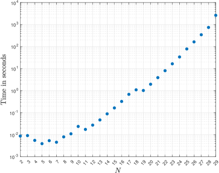
In order to understand the effect of the number of dimensions $N$ on the speed, we have generated randomly $N$ complex matrices $\mathbf{A}_{j}$ of order $2$, for $N\in\{2,3,\ldots,29\}$, and an $N$-dimensional array $\mathbf{X}\in\mathbb{C}^{2\times 2\times\ldots\times 2}$. After computing the corresponding $\mathbf{B}$, according to (4), we have obtained $X_{num}$, and computed $\|\operatorname{vec}(\mathbf{X})-\operatorname{vec}(\mathbf{X}_{num})\|_{\infty}$, which has been lower than $10^{-14}$ in all cases. In Figureย 1, we show the elapsed time in semilogarithmic scale, which is roughly linear, in agreement with the results in Sectionย 2.1. Note that both X and B in the $29$-dimensional case occupy $2^{29}\times 16=8589934592$ bytes of memory, i.e., $8$ gigabytes each of them. Therefore, the codes are able to handle massive problems, provided that the amount of memory available is large enough, and the number of dimensions seems to have no effect on the numerical stability and on the accuracy. Indeed, we remark that $N=29$ dimensions is a number much higher that what usually appears in the literature.

Refer to caption
Figure 1: Elapsed time need to solve an $N$-dimensional problem, where $\mathbf{X}\in\mathbb{C}^{2\times 2\times\ldots\times 2}$.

5.1 $N$-dimensional systems of ODEs

In order to test Theoremย 3.1, we have considered a $7$-dimensional example. More precisely, we have chosen $N=7$, $\mathbf{X}\in\mathbb{C}^{2\times 3\times 4\times 5\times 6\times 7\times 8}$, generated randomly $\mathbf{A}_{1},\mathbf{A}_{2},\ldots,\mathbf{A}_{7}$, $\mathbf{B}$ and $\mathbf{X}_{0}$, and approximated the solution of $\mathbf{X}_{t}=\sum_{j=1}^{7}\mathbf{A}_{j}\square_{j}\mathbf{X}+\mathbf{B}$, at $t=0.1$ by means of the Matlab program evolND.m, obtaining X_sylv, and also by means of a fourth-order Runge-Kutta method, obtaining X_RK. Then, we have computed the discrepancy between both numerical approximations, by means of norm(X_RK(:)-X_Sylv(:),inf). We give the whole code in Listingย 5. Note that the errors change slightly at each execution, and that the computational cost of the Runge-Kutta greatly depends on $\Delta t$. In this example, we have found that taking $\Delta t=2.5\times 10^{-5}$ gives a discrepancy of the order $10^{-14}$, but $25.61$ seconds have been needed to generate X_RK, whereas X_sylv has need only $0.06$ seconds. Obviously, a larger $\Delta t$ reduces the time to compute X_RK, but the discrepancy increases.

Listingย 5: Matlab program evolNDtest.m, that compares the Matlab function evolND with a fourth-order Runge-Kutta method
clear
t=0.1; % final time
NN=[2 3 4 5 6 7 8]; % size of $\mathbf X$
N=length(NN); % $N$
AA=cell(1,length(NN)); % matrices $\mathbf A_j$
for m=1:length(NN)
AA{m}=rand(NN(m))+1i*rand(NN(m));
end
B=rand(NN)+1i*rand(NN); % $\mathbf B$
X0=rand(NN)+1i*rand(NN); % initial data $\mathbf X_0$
tic
X_Sylv=evolND(AA,B,X0,t); % compute the solution using Theorem 1
toc,tic % elapsed time
mmax=4000; % number of time steps
dt=t/mmax; % $\Delta t$
X_RK=X0; % compute the solution using a fourth-order Runge-Kutta
for m=1:mmax
k1X=B;
for j=1:N
k1X=k1X+multND(AA{j},X_RK,j);
end
Xaux=X_RK+.5*dt*k1X;
k2X=B;
for j=1:N
k2X=k2X+multND(AA{j},Xaux,j);
end
Xaux=X_RK+.5*dt*k2X;
k3X=B;
for j=1:N
k3X=k3X+multND(AA{j},Xaux,j);
end
Xaux=X_RK+dt*k3X;
k4X=B;
for j=1:N
k4X=k4X+multND(AA{j},Xaux,j);
end
X_RK=X_RK+dt*(k1X+2*k2X+2*k3X+k4X)/6;
end
toc % elapsed time
disp(norm(X_RK(:)-X_Sylv(:),inf)) % maximum discrepancy

5.2 An advection-diffusion problem

The methods in this paper can be also used to simulate evolutionary partial differential equations. For instance, let us consider the following advection-diffusion equation:

$$\left\{\begin{aligned} &u_{t}(\mathbf{x},t)=\Delta u(\mathbf{x},t)+2\mathbf{x}\cdot\nabla u(\mathbf{x},t)+(2N+1)u(\mathbf{x},t)-\exp(-\mathbf{x}\cdot\mathbf{x}),&&\mathbf{x}\in\mathbb{R}^{N},t>0,\\ &u(\mathbf{x},0)=\exp(-\mathbf{x}\cdot\mathbf{x}),\end{aligned}\right.$$ (23)

where the diffusive term is $\Delta u=\partial^{2}u/\partial x_{1}^{2}+\partial^{2}u/\partial x_{2}^{2}+\ldots+\partial^{2}u/\partial x_{N}^{2}$, and the advective term is $2\mathbf{x}\cdot\nabla u=2(x_{1}\partial u/\partial x_{1},x_{2}\partial u/\partial x_{2},\ldots,x_{N}\partial u/\partial x_{N})$. Moreover, the solution of (23) is $u(\mathbf{x},t)=(1+\exp(t))\exp(-\mathbf{x}\cdot\mathbf{x})$.

In order to approximate numerically the spatial partial derivatives, we have used the Hermite differentiation matrices generated by the Matlab function herdif (see [15]), that are based on the Hermite functions:

$$\psi_{n}(x)=\frac{e^{-x^{2}/2}}{\pi^{1/4}\sqrt{2^{n}n!}}H_{n}(x),$$

where $H_{n}(x)$ are the Hermite polynomials:

$$H_{n}(x)=\frac{(-1)^{n}}{2^{n}}e^{x^{2}}\frac{d^{n}}{dx^{n}}e^{-x^{2}}.$$

In this example, in order to generate the first- and second-order differentiation matrices, we have typed [x,DD]=herdif(M,2,1.4);, where $M$ is the order of the differentiation matrices, $b=1.4$ is the scale factor that we have chosen, and $x$ are the Hermite nodes, i.e., the $M$ roots of $H_{n}(x)$, divided by $b$.

Hermite functions work well for problems with exponential decay. For instance, if we want to differentiate numerically $\exp(-x^{2})$ once and twice, and measure the error in discrete $L^{\infty}$-norm, it is enough to type

M=16;
[x,DD]=herdif(M,2,1.4);
D1=DD(:,:,1); % first-order differentiation matrix
D2=DD(:,:,2); % second-order differentiation matrix
norm(D1*exp(-x.^2)-(-2*x.*exp(-x.^2)),inf)
norm(D2*exp(-x.^2)-((4*x.^2-2).*exp(-x.^2)),inf)

obtaining respectively $1.2212\times 10^{-15}$ and $1.4544\times 10^{-14}$.

For the sake of simplicity, we have chosen the same number of Hermite nodes, i.e., $M=16$, and the same scale factor $b=1.4$ when discretizing all the space variables $x_{1},x_{2},\ldots,x_{N}$, but it is straightforward to consider different numbers of nodes and scale factors. In this way, we can define $\mathbf{A}=\mathbf{A}_{1}=\mathbf{A}_{2}=\ldots=\mathbf{A}_{N}$ by typing A=D2+2*diag(x)*D1+((2*N+1)/N)*eye(M);. Note that D2*U corresponds to $\partial^{2}u/\partial x_{j}^{2}$ in (23); โ€”2*diag(x)*D1*U, to $-2x_{j}\partial u/\partial x_{j}$, and ((2*N+1)/N)*eye(M)*U corresponds to $((2N+1)/N)u$, because we have divided the term $(2N+1)u$ in $N$ equal pieces, and assigned each piece to a matrix $\mathbf{A}_{j}$. With respect to B, that corresponds to the term $-\exp(-\mathbf{x}\cdot\mathbf{x})$, the simplest option is to create an $N$-dimensional mesh, which can be generated in Matlab by typing XX = cell(1, N);, followed by [XX{:}] = ndgrid(x);. This syntax is specially useful, since it allows considering different values of $N$, without modifying the code. Then, XX{1} corresponds to $x_{1}$, XX{2}, to $x_{2}$, and so on, and it is straightforward to generate B, after which XX, which requires $N$ times as much storage as U and is no longer used, can be removed from memory.

Bearing in mind all the previous arguments, it is straightforward to implement a Matlab code, which is offered in Listingย 6. Note that we impose that the numerical solution is real, to get rid of infinitesimally small imaginary components that might appear. The solution at $t=1$, taking $N=6$ dimensions, took $25.73$ seconds to execute, and the error was $9.6811\times 10^{-14}$, which, in our opinion, is quite remarkable.

Listingย 6: Matlab program advdiftest.m, that solves numerically the advection-diffusion problem (23)
clear
tic
t=1; % time at which the numerical solution will be computed
N=6; % number of dimensions $N$
M=16; % number of nodes at each dimension
[x,DD]=herdif(M,2,1.4); % create $\mathbf x$ and the differentiation matrices
D1=DD(:,:,1); % first-order differentiation matrix
D2=DD(:,:,2); % second-order differentiation matrix
AA=cell(1,N); % stores the matrices $\mathbf A_j$
XX=cell(1,N); % stores the spatial mesh
[XX{:}]=ndgrid(x); % creates the spatial mesh
B=-exp(-XX{1}.^2); % creates $\mathbf B$
for m=2:N
B=B.*exp(-XX{m}.^2);
end
clear XX % we do not need XX any more
U0=-2*B; % initial data
Uexact=-(1+exp(t))*B; % exact solution at time $t$
A=D2+2*diag(x)*D1+((2*N+1)/N)*eye(M); % creates $\mathbf A_j$
for m=1:N
AA{m}=A;
end
U=real(evolND(AA,B,U0,t)); % computes the solution at time $t$
norm(U(:)-Uexact(:),inf) % error
toc % elapsed time

Funding

This work was partially supported by the research group grant IT1615-22 funded by the Basque Government, and by the project PID2021-126813NB-I00 funded by MICIU/AEI/10.13039/501100011033 and by โ€œERDF A way of making Europeโ€.

References

  • [1] R.ย H. Bartels and G.ย W. Stewart. Solution of the matrix equation $AX+XB=C$. Communications of the ACM, 15(9):820โ€“826, 1972.
  • [2] Rajendra Bhatia and Peter Rosenthal. How and Why to Solve the Operator Equation $AX-XB=Y$. Bulletin of the London Mathematical Society, 29(1):1โ€“21, 1997.
  • [3] Minhong Chen and Daniel Kressner. Recursive blocked algorithms for linear systems with Kronecker product structure. Numerical Algorithms, 84:1199โ€“1216, 2020.
  • [4] Yuhan Chen and Chenliang Li. A Tensor Multigrid Method for Solving Sylvester Tensor Equations. IEEE Transactions on Automation Science and Engineering, 21(3):4397โ€“4405, 2024.
  • [5] Francisco deย la Hoz and Fernando Vadillo. A Sylvester-Based IMEX Method via Differentiation Matrices for Solving Nonlinear Parabolic Equations. Communications in Computational Physics, 14(4):1001โ€“1026, 2013.
  • [6] Francisco deย la Hoz and Fernando Vadillo. The solution of two-dimensional advection-diffusion equations via operational matrices. Applied Numerical Mathematics, 72:172โ€“187, 2013.
  • [7] L.ย Grasedyck. Existence and Computation of Low Kronecker-Rank Approximations for Large Linear Systems of Tensor Product Structure. Computing, 72:247โ€“265, 2004.
  • [8] Nicholasย J. Higham. Functions of Matrices. Theory and Computation. Society for Industrial and Applied Mathematics, 2008.
  • [9] Ben-Wen Li, Shuai Tian, Ya-Song Sun, and Zhang-Mao Hu. Schur-decomposition for 3D matrix equations and its application in solving radiative discrete ordinates equations discretized by Chebyshev collocation spectral method. Journal of Computational Physics, 229(4):1198โ€“1212, 2010.
  • [10] S.ย Massei and L.ย Robol. A nested divide-and-conquer method for tensor Sylvester equations with positive definite hierarchically semiseparable coefficients. IMA Journal of Numerical Analysis, 44(6):3482โ€“3519, 2024.
  • [11] B.ย N. Parlett. A recurrence among the elements of functions of triangular matrices. Linear Algebra and its Applications, 14(2):117โ€“121, 1976.
  • [12] G.ย W. Stewart. Stochastic Automata, Tensors Operation, and Matrix Equations, 1996. Technical Report, University of Maryland, UMIACS TR-96-11, CMSC TR-3598.
  • [13] Jamesย Joseph Sylvester. Sur lโ€™รฉquation en matrices $px=xq$. Comptes Rendus de lโ€™Acadรฉmie des Sciences, 99(2):67โ€“71, 115โ€“116, 1884. in French.
  • [14] Abderezak Touzene. Approximated Tensor Sum Preconditioner for Stochastic Automata Networks. In IPDPSโ€™06: Proceedings of the 20th international conference on Parallel and distributed processing, 2006.
  • [15] J.ย A.ย C. Weideman and S.ย C. Reddy. A MATLAB differentiation matrix suite. ACM Transactions on Mathematical Software, 26(4):465โ€“519, 2000. The codes are available at https://appliedmaths.sun.ac.za/$\sim$weideman/research/differ.html.
  • [16] Xin-Fang Zhang and Qing-Wen Wang. Developing iterative algorithms to solve Sylvester tensor equations. Applied Mathematics and Computation, 409:126403, 2021.