Enhancing Generalized Few-Shot Semantic Segmentation via
Effective Knowledge Transfer

Abstract

Generalized few-shot semantic segmentation (GFSS) aims to segment objects of both base and novel classes, using sufficient samples of base classes and few samples of novel classes. Representative GFSS approaches typically employ a two-phase training scheme, involving base class pre-training followed by novel class fine-tuning, to learn the classifiers for base and novel classes respectively. Nevertheless, distribution gap exists between base and novel classes in this process. To narrow this gap, we exploit effective knowledge transfer from base to novel classes. First, a novel prototype modulation module is designed to modulate novel class prototypes by exploiting the correlations between base and novel classes. Second, a novel classifier calibration module is proposed to calibrate the weight distribution of the novel classifier according to that of the base classifier. Furthermore, existing GFSS approaches suffer from a lack of contextual information for novel classes due to their limited samples, we thereby introduce a context consistency learning scheme to transfer the contextual knowledge from base to novel classes. Extensive experiments on PASCAL-5ⁱ and COCO-20ⁱ demonstrate that our approach significantly enhances the state of the art in the GFSS setting. The code is available at: https://github.com/HHHHedy/GFSS-EKT.

1 Introduction

Semantic segmentation is a fundamental computer vision task with widespread applications in fields like robotics and medical imaging. The advent of fully convolutional network (FCN) and vision transformer (ViT) has led to significant achievements in semantic segmentation (Yu and Koltun 2015; Zhao et al. 2017; Li et al. 2022; Zhang et al. 2022). However, supervised learning for this task typically demands a large amount of annotated data yet the trained models cannot recognize novel classes. To mitigate this, few-shot semantic segmentation (FSS) has been proposed to develop models that can effectively segment objects of novel classes using only a handful of annotated support samples. Recently, FSS methods (Wang et al. 2019; Lang et al. 2023; Liu and Qin 2020; Li et al. 2021; Chen and Shi 2024) have achieved significant progress; but they are constrained to segment only objects of novel classes while ignoring base classes. To overcome this limitation, generalized few-shot semantic segmentation (GFSS) extends FSS to segment both base and novel classes.

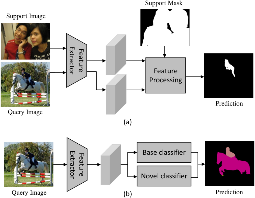
Figure 1: Illustration of (a) FSS and (b) GFSS: FSS models predict only the novel class specified by the support image, whereas GFSS models can predict both base and novel classes at the same time. During inference, GFSS models do not rely on support images of novel classes any more, as they are fine-tuned using all samples of novel classes to form a novel classifier. In this context, “horse” is a base class, while “person” represents a novel class.

Representative GFSS approaches (Tian et al. 2022; Liu et al. 2023; Hajimiri et al. 2023; Lu et al. 2023; Zhang et al. 2024) adopt a two-phase training process: in the pre-training phase, the model is trained on sufficient base samples to segment objects of base classes; afterward, in the fine-tuning phase, the model is updated with a few annotated samples of novel classes, enabling simultaneous segmentation of both base and novel classes. Figure 1 illustrates the comparison between FSS and GFSS. This two-phase training approach often results in poor performance on novel classes due to the distribution gap between base and novel classes. This distribution gap causes the feature extractor and base classifier, which are pre-trained on abundant samples of base classes, to fail in effectively capturing the features of novel classes and successfully segmenting novel classes within images. A typical solution is to fine-tune the feature extractor and base classifier using the limited novel samples available; however, this can lead to performance degradation on the base classes. While training a separate novel classifier is possible, achieving balanced base and novel classifiers simultaneously remain challenging.

In this work, we propose an Effective Knowledge Transfer approach for enhancing GFSS, namely GFSS-EKT, to prevent performance degradation on base classes and improve performance on novel classes. Our method employs a two-phase training scheme. In the pre-training phase, we extract features from input base class samples using a feature extractor and decompose them by projecting them onto learnable base prototypes representing different classes. Then, a base classifier is trained to perform a classification on base classes. The same feature extraction is used in the fine-tuning phase, the features of novel class samples are decomposed by both base and novel prototypes. A novel classifier is then learned alongside the base classifier to classify both base and novel classes. We make three main contributions. First, we propose a novel prototype modulation module that adjusts novel class prototypes by leveraging their correlations with base class prototypes. Second, we introduce a novel classifier calibration module that adjusts the weight distribution of the novel classifier through mean shifting and standard deviation scaling, obtaining a more reliable novel classifier. Finally, current GFSS approaches face the challenge of lacking contextual information for novel classes when fine-tuning models with few novel samples. To tackle it, we incorporate base samples into the fine-tuning phase and introduce a context consistency learning scheme between two augmented versions of a given base sample. The augmentation operations are carefully designed to focus on the meaningful contextual part of the base image so that the relevant knowledge can be transferred from the base to novel classes.

We evaluate our method on two public datasets, PASCAL-5ⁱ and COCO-20ⁱ. The experimental results demonstrate that our method achieves significant improvement over the state of the art.

2 Related Work

Semantic Segmentation.

Semantic segmentation is to classify each pixel of the image into specific class. Since the emergence of fully convolutional network (FCN) (Long, Shelhamer, and Darrell 2015), semantic segmentation has achieved remarkable progress thanks to various advanced techniques. For instance, dilated convolution (Yu and Koltun 2015), pyramid pooling module (Zhao et al. 2017), atrous spatial pyramid pooling (Chen et al. 2017), etc. have been proposed to handle varying object sizes in images. Besides, some transformer-based FSS models (Hu, Sun, and Yang 2022; Lu et al. 2021; Zhang et al. 2021, 2022) have also been proposed since the advent of ViT (Dosovitskiy et al. 2020) in computer vision. For example, MM-Former (Zhang et al. 2022) employs Mask2Former (Cheng et al. 2022) to generate multiple mask proposals for the query image. Despite the success of these methods, they generally require a large amount of training data to achieve good performance.

Few-Shot Semantic Segmentation.

Few-shot semantic segmentation (FSS) aims to segment novel classes given a few support samples, which alleviates the dependence of the segmentation model on a large amount of training data. Previous FSS approaches (Wang et al. 2019; Liu and Qin 2020; Lang et al. 2023; Li et al. 2021; Chen et al. 2023) typically employ the episodic learning that organizes the base data into multiple episodes, each of which consists of a query image and few support images of the same base class to simulate the few-shot scenario for novel classes. They normally utilize the information contained in annotated support images of a certain class to perform pixel-wise classification on the query image via non-parametric similarity measurement (Wang et al. 2019; Liu and Qin 2020) or parametric decoder (Lang et al. 2023; Li et al. 2021; Zhang, Shi, and Li 2022). Current FSS approaches cannot identify base and novel classes simultaneously.

Generalized Few-Shot Learning.

Generalized few-shot learning (GFSL) extends FSS by equipping the model with the ability of recognizing the novel classes with few samples while preserving the ability of recognizing base classes. For instance, Kim et al. (Kim and Choi 2023) propose to apply weight normalization to both base and novel classifiers so as to achieve balanced decision boundaries for both base and novel classes. Generalized few-shot semantic segmentation (GFSS) is an application of GFSL in semantic segmentation. GFSS methods like CAPL (Tian et al. 2022) and PKL (Huang et al. 2023) leverage abundant base samples to train base prototypes; subsequently, novel prototypes are generated directly from the support samples of novel classes to work with base prototypes as joint classifiers. On the other hand, approaches such as POP (Liu et al. 2023), DIaM (Hajimiri et al. 2023), and BCM (Sakai et al. 2024) employ a two-phase training scheme to train both base and novel classifiers. In the pre-training phase, the base classifier is trained with sufficient base samples. In the fine-tuning phase, DIaM (Hajimiri et al. 2023) and BCM (Sakai et al. 2024) train the novel classifier using only novel samples, while POP (Liu et al. 2023) uses both base and novel samples.

Following (Kim and Choi 2023; Liu et al. 2023; Hajimiri et al. 2023; Sakai et al. 2024), our method is built with the two-phase training scheme. We aim to overcome the data imbalance and distribution gap between base and novel classes by effectively transferring the knowledge from base to novel classes, through three new modules, i.e. novel prototype modulation, novel classifier calibration, and context consistency learning.

3 Method

3.1 Problem Definition

For generalized few-shot semantic segmentation, the training data set consists of a base set $D_{base}$ involving $M$ base classes $C_{base}$ with abundant annotated images and a novel set $D_{novel}$ including $N$ novel classes $C_{novel}$ with a few annotated images per class. Note that $C_{base}\cap C_{novel}=\emptyset$.

3.2 Method Overview

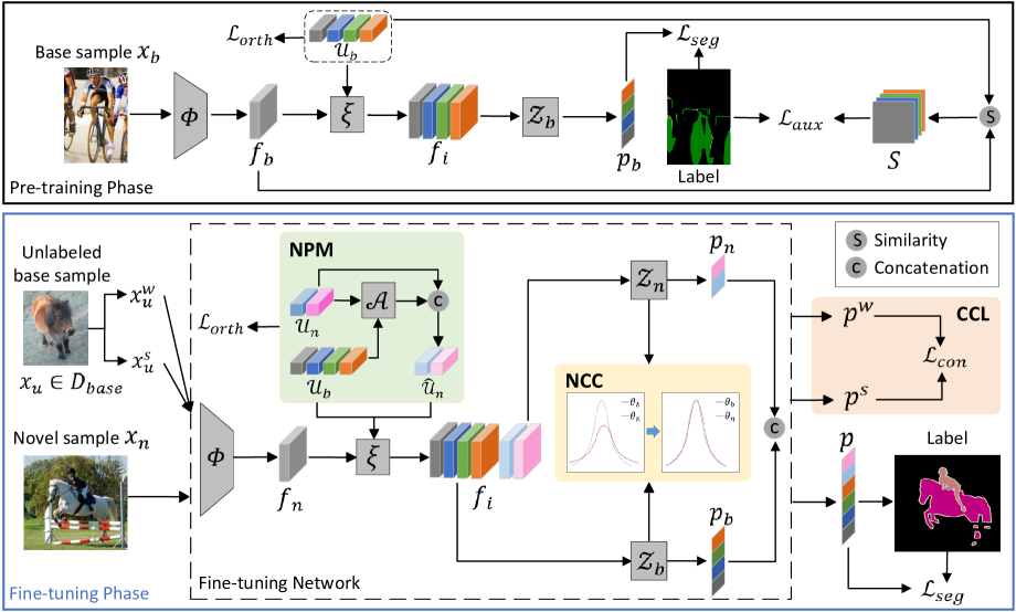
Figure 2: Overview of our model. Novel prototype modulation (NPM) module, novel classifier calibration (NCC) module, and context consistency loss (CCL) module are shown in the boxes with green, yellow, and orange backgrounds respectively.

Figure 2 illustrates an overview of our proposed method. It follows two-phase framework and involves three new modules, i.e. novel prototype modulation (NPM, Sec. 3.3), novel classifier calibration (NCC, Sec. 3.4), and context consistency learning (CCL, Sec. 3.5). Specifically, in the pre-training phase, given a base sample $x_{b}$, we extract its feature $f_{b}$ using the feature extractor $\Phi$. $f_{b}$ is then fed into the feature decomposer $\xi$ similar to (Liu et al. 2023), where $f_{b}$ is decomposed into $M+1$ sub-features $\{f_{i}\}_{i=0}^{M}$ by projecting it onto base prototypes $\mathcal{U}_{b}$. Each sub-feature $f_{i}$ is the feature representation for the $i$-th class, and $f_{0}=f_{b}-\sum\nolimits_{i=1}^{M}f_{i}$ is the background representation. $\mathcal{U}_{b}=\{u_{i}\}_{i=1}^{M}$ are randomly initialized and updated in the model. Afterward, these sub-features are passed through a learnable base classifier $\mathcal{Z}_{b}$ to obtain the predicted probability $p_{b}$ for the per-pixel classification of $x_{b}$. In the fine-tuning phase, given a novel sample $x_{n}$, we similarly extract its feature $f_{n}$ using $\Phi$ and decompose it into $M+N+1$ sub-features $\{f_{i}\}_{i=0}^{M+N}$ by projecting it onto well-learned base prototypes $\mathcal{U}_{b}$ and randomly initialized novel prototypes $\mathcal{U}_{n}=\{u_{i}\}_{i=M+1}^{M+N}$, and $f_{0}=f_{n}-\sum\nolimits_{i=1}^{M+N}f_{i}$. These sub-features are then fed into both the base classifier $\mathcal{Z}_{b}$ and the novel classifier $\mathcal{Z}_{n}$. Similar to $\mathcal{Z}_{b}$, $\mathcal{Z}_{n}$ produces the per-pixel classification result $p_{n}$ on novel classes; the final predicted probability $p$, is thereby a combination of $p_{b}$ and $p_{n}$. Last, two augmented versions (i.e. , $x_{u}^{w}$ and $x_{u}^{s}$) of an unlabeled base sample are processed to compute a consistency loss. Specifically, our proposed modules are all implemented during the fine-tuning phase: 1) NPM is utilized to refine $\mathcal{U}_{n}$ by transferring knowledge from $\mathcal{U}_{b}$ to $\mathcal{U}_{n}$ through the attention mechanism $\mathcal{A}$; 2) NCC is proposed to calibrate $\mathcal{Z}_{n}$ according to the weight distributions of $\mathcal{Z}_{b}$ and $\mathcal{Z}_{n}$; 3) CCL is introduced between $x_{u}^{w}$ and $x_{u}^{s}$ to reinforce their context consistency and transfer it from base to novel classes.

3.3 Novel Prototype Modulation

Given sufficient base data, the model effectively learns distinct prototypes for base classes; however, it is challenging to learn such novel prototypes given limited novel samples. In fact, novel classes may likely share elemental patterns with base classes (Wu et al. 2021), we propose to modulate novel prototypes by exploiting their correlations to base prototypes, so as to compensate for the knowledge insufficiency in novel samples.

To capture the correlative information between base and novel classes, we employ the cross-attention mechanism to compute a weighted sum of base prototypes for each novel class. For each novel prototype $u_{i}\in\mathcal{U}_{n}$, it can be reconstructed as a result of the weighted sum of all base prototypes $\mathcal{U}_{b}$:

$$\begin{split}&\mathcal{A}(u_{i},\mathcal{U}_{b})=Softmax(QK^{T})V,\\ &Q,K,V=u_{i}W^{Q},\mathcal{U}_{b}W^{K},\mathcal{U}_{b}W^{V}\\ \end{split}$$ (1)

where $W^{Q}$, $W^{K}$, $W^{V}$ are three linear layers. $\mathcal{A}(u_{i},\mathcal{U}_{b})$ is the reconstructed novel prototype encoded with its correlation to base prototypes.

Subsequently, we modulate the original novel prototype by fusing it with the reconstructed one through concatenation followed by a linear layer. This process generates new prototypes $\hat{\mathcal{U}}_{n}$ which replace the original $\mathcal{U}_{n}$, preserving the uniqueness of novel classes and their connections to base classes.

3.4 Novel Classifier Calibration

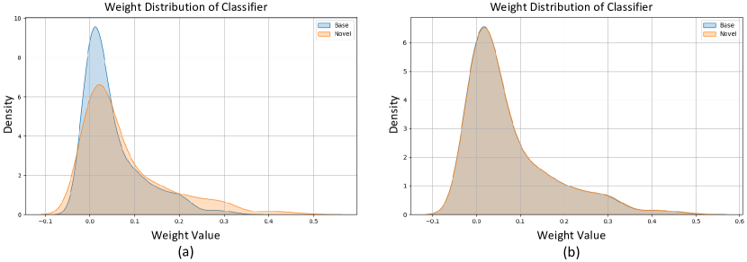
Figure 3: (a) illustrates the weight distributions of two classifiers without NCC; (b) shows their weight distributions after implementing NCC.

When fine-tuning the model on novel classes with only few support samples, the novel classifier is prone to overfitting. In contrast, the base classifier originally trained with sufficient base data is more reliable. The performance on both base and novel classes can be negatively impacted, whilst previous approaches often ignore this. We propose to leverage the knowledge in base classifier to aid in training the novel classifier.

As reported in (Kim and Choi 2023), the position and shape of a decision boundary, which separates different classes in the feature space, are determined by the classifier’s weight distribution. Our observation (see Figure 3) indicates that the base classifier exhibits a more centric weight distribution; while that of the novel classifier has a larger variance, resulting in potential prediction bias towards it. To address this issue, we calibrate the weight distribution of the novel classifier to align with that of the base classifier. This way can effectively improve the generalization ability of the novel classifier.

We investigate the underlying weight distributions of base and novel classifiers by their means and standard deviations. More specifically, the weights of the base classifier and novel classifier are denoted as $\mathcal{Z}_{b}=\{\theta_{i}\}_{i=1}^{M}\in\mathbb{R}^{d\times M}$ and $\mathcal{Z}_{n}=\{\theta_{i}\}_{i=M+1}^{M+N}\in\mathbb{R}^{d\times N}$, respectively; $\theta_{i}\in\mathbb{R}^{d}$ represents the weight vector for class $i$. We calculate the mean and standard deviation for the weight vector in the channel direction: $\mu_{i}=\frac{1}{d}\sum\nolimits_{j=1}^{d}\theta_{ij}$ and $\sigma_{i}=\sqrt{\frac{1}{d}\sum\nolimits_{j=1}^{d}(\theta_{ij}-\mu_{i})}$. Afterward, the average of means and standard deviations over base classes can be given by: $\overline{\mu}_{b}=\frac{1}{M}\sum\nolimits_{i=1}^{M}\mu_{i}$ and $\overline{\sigma}_{b}=\frac{1}{M}\sum_{i=1}^{M}\sigma_{i}$. Similarly, $\mu_{n}$, $\sigma_{n}$, $\overline{\mu}_{n}$ and $\overline{\sigma}_{n}$ for the novel classifier $\mathcal{Z}_{n}$ can be calculated following the same way.

To calibrate the novel classifier, we adjust $\mathcal{Z}_{n}$ by first centering it and then shifting it to be in line with $\overline{\mu}_{b}$:

$$\hat{\mathcal{Z}}_{n}=\mathcal{Z}_{n}-\overline{\mu}_{n}+\overline{\mu}_{b}$$ (2)

where $\overline{\mu}_{n}$ and $\overline{\mu}_{b}$ denote the average of means for novel classes and base classes, respectively; they are replicated for subtraction. Secondly, we adjust $\hat{\mathcal{Z}}_{n}$ by scaling it according to the ratio of $\overline{\sigma}_{b}$ to $\sigma_{n}$:

$$\hat{\mathcal{Z}}_{n}=\frac{\overline{\sigma}_{b}}{\sigma_{n}}\hat{\mathcal{Z}}_{n}$$ (3)

The calibration happens during the fine-tuning phase after every epoch.

3.5 Context Consistency Learning

$K$-shot support samples of novel classes provide very limited contextual information for the class. Nonetheless, base and novel classes may likely share similar contexts. To further leverage base samples for improving the learning of novel classes, we introduce a context consistency learning scheme by incorporating the base samples into the fine-tuning phase following an unsupervised manner.

Directly incorporating the base samples with labels into the fine-tuning phase would bias the model towards base classes. Inspired by the consistency learning techniques widely used in semi-supervised learning works (Sohn et al. 2020; Wei et al. 2023; Ouali, Hudelot, and Tami 2020), that is a robust model should yield similar outputs for different perturbed versions of the same image, we introduce a context consistency learning scheme. As illustrated in Figure 2 , for a given base image $x_{u}$, we generate a weakly-augmented version $x_{u}^{w}$ using simple augmentation operation, i.e. , flipping and cropping, and a strongly-augmented version $x_{u}^{s}$ by applying additional augmentation, i.e. , cutout, on top of the weakly-augmented version.

Augmentation like cutout in representative semi-supervised works (Sohn et al. 2020; Ouali, Hudelot, and Tami 2020) is normally performed randomly on the image without constraints. However, this operation often fails to capture meaningful information. To let the model specifically focus on the contextual part of the image, we instead introduce a context-oriented augmentation operation: first, we take the bounding box of the ground truth mask for each object class in the image (note that one bounding box is generated when multiple objects of the same class can form a single connected component); second, we randomly select a pixel from the bounding box boundaries of all classes, serving as the center of a $16\times 16$ squared cutout region. This is because, in the image, pure backgrounds, e.g. , grass, and sky, are too simple context for consistency learning, while cutout purely within the objects lacks contextual information for knowledge transfer. Therefore, we select regions close to or with a partial of the objects.

Let $p^{w}$ and $p^{s}$ denote the predicted probabilities output by the segmentation model for $x_{u}^{w}$ and $x_{u}^{s}$, respectively. We compute the cross-entropy loss between $p^{w}$ and $p^{s}$ for consistency as follows:

$$\mathcal{L}_{con}=\frac{1}{H\times W}\sum_{i=1}^{H\times W}-p_{i}^{w}\log(p_{i}^{s})$$ (4)

where $H\times W$ is the number of pixels in the image.

3.6 Optimization

Phase 1: Pre-Training.

In this phase, we only use the base set $D_{base}$ to train the network including the feature extractor $\Phi$, base classifier $\mathcal{Z}_{b}$ and base prototypes $\mathcal{U}_{b}$ in the feature decomposer $\xi$. Following previous works (Tian et al. 2022; Liu et al. 2023; Kim and Choi 2023), we calculate the segmentation loss $\mathcal{L}_{seg}$ (a cross-entropy loss) and the orthogonal loss $\mathcal{L}_{orth}=\sum_{i\neq j}|u_{i}\cdot u_{j}^{T}|$ ($u_{i},u_{j}\in\{\mathcal{U}_{b},\mathcal{U}_{n}\}$).

In addition, we introduce an auxiliary loss $\mathcal{L}_{aux}$: we use base prototypes $\mathcal{U}_{b}$ as if they were a base classifier to classify the image feature $f_{b}$ by computing the similarity between $\mathcal{U}_{b}$ and $f_{b}$, and the output result is optimized with the ground truth using the cross-entropy loss (see Figure 2). $\mathcal{L}_{aux}$ used in the pre-training phase boosts performance on base classes, as evidenced by the results in both 1-shot and 5-shot settings shown in Table 3. The total training loss is: $\mathcal{L}_{total}=\mathcal{L}_{seg}+\mathcal{L}_{orth}+\mathcal{L}_{aux}$.

Phase 2: Fine-Tuning.

In this phase, the model is updated with support samples of novel classes alongside unlabeled base samples from $D_{base}$. We first freeze all modules learned in the pre-training phase and then train novel prototypes and novel classifier. The training loss during this phase contains three components, defined as: $\mathcal{L}_{total}=\mathcal{L}_{seg}+\mathcal{L}_{orth}+\mathcal{L}_{con}$, where $\mathcal{L}_{con}$ is the consistency loss shown in Sec. 3.5.

4 Experiments

4.1 Datasets and Evaluation Metric

Datasets.

We evaluate our model on two public datasets, PASCAL-5ⁱ (Shaban et al. 2017) and COCO-20ⁱ (Nguyen and Todorovic 2019). PASCAL-5ⁱ comprises 20 categories and COCO-20ⁱ consists of 80 categories. Object categories in each dataset are evenly split into four folds. Following (Tian et al. 2022), we adopt a cross-validation manner to train the model on three folds while testing on one fold. This procedure is repeated four times, and we report the average result. We perform $K\in\{1,5\}$ shot semantic segmentation.

Evaluation Metric.

Following previous approaches (Tian et al. 2022; Liu et al. 2023), the mean intersection-over-union (mIoU) is adopted as the evaluation metric. $mIoU=\frac{1}{C}\sum\nolimits^{C}_{i=0}IoU_{i}$, where $C$ is the number of classes, and $IoU_{i}$ denotes the intersection-over-union between the predicted segmentation mask and ground truth mask for the $i$-th novel class. To comprehensively evaluate our results, we calculate the average $mIoU$ over the four times validation, denoted by $\overline{mIoU}_{base}$ and $\overline{mIoU}_{novel}$ for the base and novel classes, respectively. Subsequently, we compute the arithmetic mean (Liu et al. 2023) (denoted as “Mean”) of the $\overline{mIoU}_{base}$ and $\overline{mIoU}_{novel}$. However, the arithmetic mean is dominated by the base classes, which are the majority. To obtain a more balanced metric, we use the harmonic mean (Huang et al. 2023) (denoted as “H-Mean”), formulated as:

$$\operatorname{H-Mean}=\frac{2\cdot\overline{mIoU}_{base}\cdot\overline{mIoU}_{novel}}{\overline{mIoU}_{base}+\overline{mIoU}_{novel}}$$ (5)

This approach addresses class unbalance in datasets such as PASCAL-5ⁱ and COCO-20ⁱ, where the number of base classes is three times than that of novel classes.

4.2 Implementation Details

We follow (Liu et al. 2023) to curate the dataset. Notably, in the pre-training phase, the pixels of novel classes in base images are treated as background. During the novel class fine-tuning phase, we randomly sample $K\in\{1,5\}$ images from novel classes as support images. All images are cropped to $473\times 473$ as input to the network during training. Our method is implemented in PyTorch with NVIDIA A100. We utilize PSPNet (Zhao et al. 2017) with ResNet50 (He et al. 2016) as the feature extractor. In the pre-training phase, the model is optimized using stochastic gradient descent (SGD) with an initial learning rate of $0.01$, a momentum of $0.9$, and a weight decay of $0.0001$. The model is trained for $50$ epochs on both datasets, and the batch size is set as 8 and 16 for PASCAL-5ⁱ and COCO-20ⁱ, respectively. In the fine-tuning phase, we update the model using SGD with a learning rate of $0.01$, training for 500 epochs on both datasets.

Methods	1-shot				5-shot
	Base	Novel	Mean	H-Mean	Base	Novel	Mean	H-Mean
CAPL (Tian et al. 2022)	65.48	18.85	54.38	29.27	66.14	22.41	55.72	33.48
PKL (Huang et al. 2023)	68.84	26.90	58.86	37.83	69.22	34.40	61.18	45.42
DIaM (Hajimiri et al. 2023)	70.89	35.11	61.95	46.96	70.85	55.31	66.97	62.12
POP (Liu et al. 2023)	73.92	35.51	64.77	47.97	74.78	55.87	70.27	63.96
BCM (Sakai et al. 2024)	71.15	41.24	64.03	52.22	71.23	55.36	67.45	62.30
Ours	75.23	43.93	67.78	55.47	75.73	57.00	71.28	65.04

Table 1: Performance comparison on PASCAL-5ⁱ

Methods	1-shot				5-shot
	Base	Novel	Mean	H-Mean	Base	Novel	Mean	H-Mean
CAPL (Tian et al. 2022)	44.61	7.05	35.46	12.18	45.24	11.05	36.80	17.76
PKL (Huang et al. 2023)	46.36	11.04	37.71	17.83	46.77	14.91	38.90	22.61
DIaM (Hajimiri et al. 2023)	48.28	17.22	39.02	25.39	48.37	28.73	38.55	36.05
POP (Liu et al. 2023)	54.71	15.31	44.98	23.92	54.90	29.97	48.75	38.77
BCM (Sakai et al. 2024)	49.43	18.28	42.01	26.69	49.88	30.60	45.29	37.93
Ours	54.81	21.83	46.96	31.22	55.68	31.62	49.95	40.33

Table 2: Performance comparison on COCO-20ⁱ

4.3 Performance Comparison

Quantitative Analysis.

$\mathcal{L}_{aux}$	NCC	CCL	NPM	1-shot				5-shot
				Base	Novel	Mean	H-Mean	Base	Novel	Mean	H-Mean
-	-	-	-	70.81	36.97	62.75	48.58	72.94	54.77	68.61	62.56
✓	-	-	-	71.40	38.82	63.64	50.29	74.06	54.62	69.44	62.87
✓	✓	-	-	75.29	39.15	66.69	51.51	75.74	53.98	70.56	63.03
✓	✓	✓	-	75.40	42.49	67.56	54.82	75.68	56.24	71.05	64.53
✓	✓	✓	✓	75.23	43.93	67.78	55.47	75.73	57.00	71.27	65.04

Table 3: Ablation study on modules. $\mathcal{L}_{aux}$ represents the auxiliary loss used in base class pre-training; NCC, CCL and NPM denote the novel classifier calibration, context consistency learning and novel prototype modulation, respectively.

Table 1 and 2 present a comparison of several GFSS methods with our method on the PASCAL-5ⁱ and COCO-20ⁱ datasets. Methods such as CAPL (Tian et al. 2022), PKL (Huang et al. 2023), DIaM (Hajimiri et al. 2023), and BCM (Sakai et al. 2024) rely solely on novel samples for novel classifier learning, whilst POP (Liu et al. 2023) and our method also use base samples in the learning process. On both datasets, our method outperforms all other methods in both 1-shot and 5-shot scenarios. Specifically, in terms of “H-Mean”, our approach achieves significant improvements over the previous best, with gains of 3.25% mIoU and 4.53% mIoU in the 1-shot setting on PASCAL-5ⁱ and COCO-20ⁱ, respectively. Furthermore, in the 5-shot setting, our method surpasses the previous best by over 1% on both datasets. Notice that our performance gain diminishes in 5-shot because the complementary knowledge provided by the base classes for novel classes becomes increasingly limited as the number of novel samples increases. These results indicate that our method performs particularly well on novel classes, demonstrating its effectiveness in enhancing knowledge transfer from base to novel classes for GFSS.

Qualitative Comparison.

Figure 4 illustrates five examples from PASCAL-5ⁱ using our method and POP (Liu et al. 2023) in the 1-shot scenario. Our method shows superior segmentation performance. For instance, the first example in the first row demonstrates the effectiveness of our method in reducing image noise; the last example indicates that our method improves the model’s ability to segment different parts of objects.

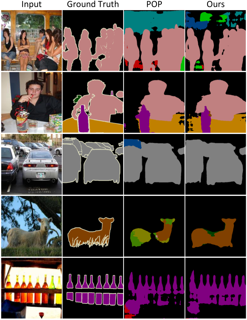
Figure 4: Qualitative results of our method and POP (Liu et al. 2023) on PASCAL-5ⁱ.

4.4 Ablation Studies

In this section, we investigate the effectiveness of each module proposed in our method by conducting a series of ablation studies on PASCAL-5ⁱ.

Novel Prototype Modulation (NPM).

Methods	1-shot
	Base	Novel	Mean	H-Mean
CS	75.44	41.32	67.32	53.39
CA	75.23	43.93	67.78	55.47

Table 4: Ablation study on the NPM. CS denotes cosine similarity, while CA denotes cross attention.

When removing NPM, a decrease of 1.44% mIoU on novel classes can be observed in Table 3, which indicates that this module effectively transfers correlation information from base to novel prototypes. To investigate NPM, we compare NPM configured with different reconstruction methods. The results in Table 4 demonstrate that using cross-attention (CA) to compute the correlation between base and novel prototypes is superior to using cosine similarity (CS). We attribute this to the strong ability of cross-attention to capture correlations between base and novel classes, thereby enhancing knowledge transfer from base to novel classes.

Novel Classifier Calibration (NCC).

Methods	1-shot
	Base	Novel	Mean	H-Mean
w/o NCC	71.40	38.82	63.64	50.29
w/ NBCC	72.61	38.34	64.56	50.18
w/ NCC	75.29	39.15	66.69	51.51

Table 5: Ablation study on NCC. NBCC denotes calibrating both base and novel classifiers.

Table 3 presents a 3.89% mIoU decrease on base classes by removing NCC and a slight drop, 0.33% mIoU, on novel classes, which demonstrates that it is effective to calibrate the weight distribution of the novel classifier, reducing its bias. To further investigate the method of novel classifier calibration, we investigate another variant such as calibrating both base and novel classifiers according to the averaged statistics of their weight distributions (NBCC). Table 5 shows that both NCC and NBCC enhance performance on base classes. However, NCC achieves more significant improvements, with a 2.68$\%$ mIoU increase on base classes and a 0.81$\%$ mIoU increase on novel classes compared to NBCC, adjusting the weight distribution of base classifier somewhat disrupts the well-learned base classifier.

Context Consistency Learning (CCL).

Methods	1-shot
	Base	Novel	Mean	H-Mean
w/ label	74.61	39.05	66.14	51.27
w/o label	75.40	42.49	67.56	54.82

Table 6: Ablation study on the CCL. Comparison between using or not using labels of base sample in fine-tuning.

Methods	1-shot
	Base	Novel	Mean	H-Mean
base $+$ novel	75.40	42.49	67.56	54.82
w/o base	75.12	36.58	65.94	49.20
w/o novel	75.04	35.30	65.57	48.01

Table 7: Ablation study on the CCL. Comparison between different classifiers.

Methods	1-shot
	Base	Novel	Mean	H-Mean
only novel	75.39	39.28	66.79	51.65
only base	75.40	42.49	67.56	54.82
base $+$ novel	75.51	41.20	67.43	53.31

Table 8: Ablation study on the CCL. Comparison between different sources of samples.

Methods	1-shot
	Base	Novel	Mean	H-Mean
Randaugment	73.06	35.91	64.36	48.15
cutout	75.40	42.49	67.56	54.82

Table 9: Ablation study on the CCL. Comparison between different augmentation techniques.

Methods	1-shot
	Base	Novel	Mean	H-Mean
wcutout	74.98	40.34	66.73	52.46
ocutout	75.17	40.62	66.94	52.74
icutout	75.07	40.46	66.83	52.58
bcutout (ours)	75.40	42.49	67.56	54.82

Table 10: Ablation study on the CCL. Comparison between different cutout methods.

In Table 3, there is a significant drop (i.e. , -3.34% mIoU) on novel classes when ablating CCL, which shows the effectiveness of this scheme. To further validate it, we conduct several experiments. In Table 6, we compare the experimental results of the fine-tuning phase using labeled or unlabeled base samples. The results indicate that the label-free method (w/o label) outperforms the labeled one (w/ label), showing improvements in both base and novel classes. This suggests that using explicit supervision for base classes during fine-tuning increases the imbalance between base and novel classes, resulting in the model biased towards base classes.

To evaluate the necessity of using both base and novel classifiers when applying consistency to base samples, we conduct an experiment that removes the base or novel classifier respectively. In Table 7, we observe that omitting either the base classifier (w/o base) or the novel classifier (w/o novel), as compared to employing both (base $+$ novel), results in a significant performance decline, which demonstrates that both the base and novel classifiers play crucial roles in the final prediction.

Furthermore, Table 8 shows the results of performing consistency learning on samples from novel/base set. The results show that using only novel samples (only novel) or using both base and novel samples (base $+$ novel) is inferior to using only base samples (only base). This is likely because novel samples are fully utilized through the supervised learning, incorporating them also in the unsupervised learning might confuse the model.

Moreover, we study the augmentation operations for context consistency learning. First, regarding the strong augmentation, instead of choosing cutout, we follow the method Randaugment (Cubuk et al. 2020) to use photometric transformations (e.g. , contrast, brightness, and sharpness). As shown in Table 9, a significant performance decrease is observed when using Randaugment. Second, we study the proposed context-oriented augmentation operation by comparing different cutout methods. Our proposed cutout is performed by randomly selecting a pixel from the bounding box boundaries to serve as the center of the cutout region (bcutout). For comparison, we consider three alternative methods: wcutout, where the cutout region is randomly selected within the bounding boxes; ocutout, where the cutout region is randomly selected outside the bounding boxes; icutout, where the cutout region is selected randomly from the entire image.

As shown in Table 10, the comparison between our proposed bcutout with the wcutout, ocutout, and icutout indicates that our bcutout outperforms the others, as the region near the bounding box boundaries contains richer contextual knowledge.

4.5 Discussion and Visualization

Class Split Analysis.

Methods	1-shot
	Base	Novel	Mean	H-Mean
Baseline	85.36	21.74	70.21	34.65
Ours	86.96	24.39	72.06	38.10

Table 11: Ablation study on a challenging split.

To evaluate the effectiveness of our method across various splits, we conduct experiments using a challenging split of PASCAL-5i with aeroplane, bicycle, boat, bus, car, motorbike, and train being novel classes, and bird, cat, cow, dog, horse, person, and sheep being base classes. The experiment is conducted in the 1-shot setting and the mIoU is reported in Table 11. The results show that our method improves both base and novel class performance over POP (Liu et al. 2023), which serves as the baseline of our method. This demonstrates that our method is effective even when base and novel classes are not intuitively correlated. This effectiveness can be attributed to the presence of shared elemental patterns in the low-level visual features (e.g. texture, shape) between base and novel classes. Furthermore, from a biomimicry perspective, the structures and functions of many man-made objects are indeed inspired by nature. For example, the connections between planes and birds, cars and horses.

t-SNE Visualization.

We utilize t-SNE to visualize all base and novel prototypes, along with the features of 20 samples per class. In Figure 5 (a), the t-SNE visualization of POP (Liu et al. 2023) is presented, where $\mathcal{U}_{b}$ and $\mathcal{U}_{n}$ denote base prototypes and novel prototypes, respectively, while $\mathcal{F}_{b}$ and $\mathcal{F}_{n}$ represent the features of base and novel classes. Similarly, Figure 5 (b) illustrates the t-SNE visualization of our proposed method using the same symbols. Despite both methods extracting features from the same structure with the same parameters, the t-SNE visualizations show that base and novel prototypes become more representative after applying our proposed method.

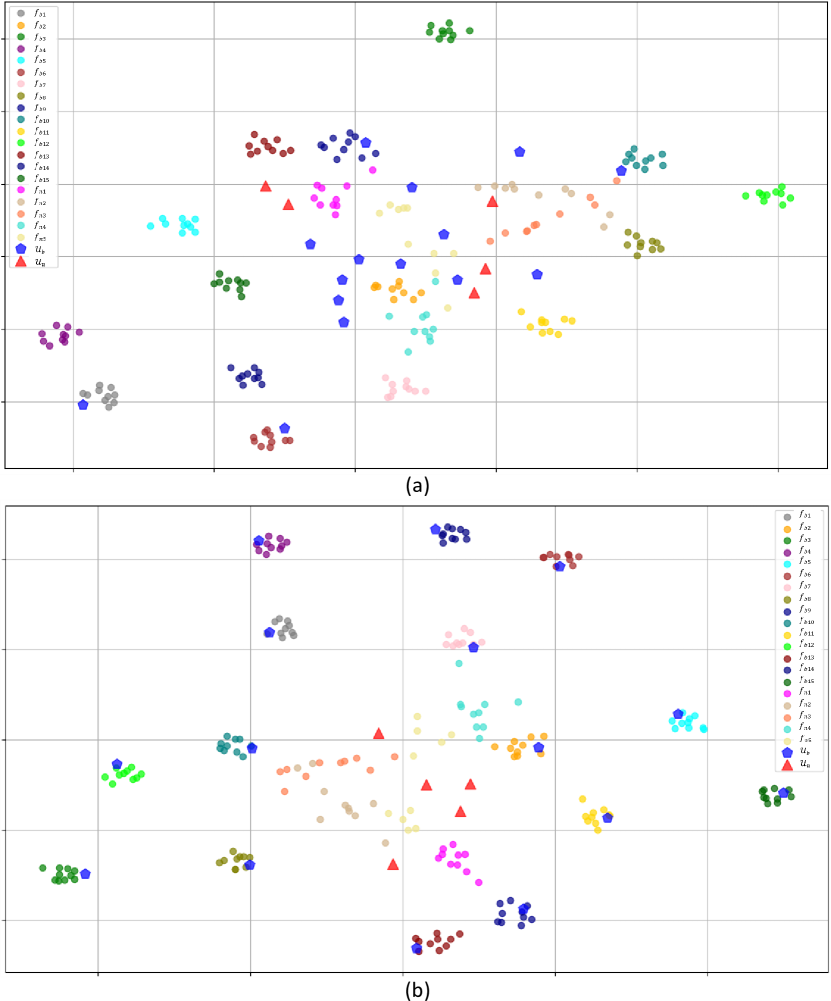
Figure 5: t-SNE visualization of features and class prototypes. (a) illustrates the t-SNE visualization of POP (Liu et al. 2023); (b) shows the t-SNE visualization of our proposed method. The base prototypes ($\mathcal{U}_{b}$) are represented as blue pentagrams, and the novel prototypes ($\mathcal{U}_{n}$) are shown as red rectangles. The features of base classes ($\mathcal{F}_{b}$) and novel classes ($\mathcal{F}_{n}$) are visualized as dots, where features of the same class are clustered and represented by dots of the same color.

5 Conclusion

In this work, we propose to enhance generalized few-shot semantic segmentation through effective knowledge transfer. During the fine-tuning stage, we design three modules to facilitate knowledge transfer from base to novel classes. First, the novel prototype modulation module is proposed to adjust the novel prototypes by exploiting their correlations with base prototypes. Second, the novel classifier calibration module aims to calibrate the weight distribution of the novel classifier using mean shifting and standard deviation scaling according to that of the base classifier. Last, to further make use of the contextual knowledge in base classes, we introduce a context consistency learning scheme to transfer the contextual information from base to novel classes. We conduct extensive experiments on PASCAL-5ⁱ and COCO-20ⁱ, which demonstrate that our method effectively improves previous GFSS approaches. Future work will focus on leveraging text information via multimodal large language model into this framework.

References

- Chen et al. (2017) Chen, L.-C.; Papandreou, G.; Kokkinos, I.; Murphy, K.; and Yuille, A. L. 2017. Deeplab: Semantic image segmentation with deep convolutional nets, atrous convolution, and fully connected crfs. IEEE transactions on pattern analysis and machine intelligence, 40(4): 834–848.
- Chen and Shi (2024) Chen, X.; and Shi, M. 2024. Memory-guided Network with Uncertainty-based Feature Augmentation for Few-shot Semantic Segmentation. In IEEE International Conference on Multimedia and Expo (ICME).
- Chen et al. (2023) Chen, X.; Wang, Y.; Xu, Y.; and Shi, M. 2023. Distilling base-and-meta network with contrastive learning for few-shot semantic segmentation. Autonomous Intelligent Systems, 3(1): 11.
- Cheng et al. (2022) Cheng, B.; Misra, I.; Schwing, A. G.; Kirillov, A.; and Girdhar, R. 2022. Masked-attention mask transformer for universal image segmentation. In Proceedings of the IEEE/CVF Conference on Computer Vision and Pattern Recognition, 1290–1299.
- Cubuk et al. (2020) Cubuk, E. D.; Zoph, B.; Shlens, J.; and Le, Q. V. 2020. Randaugment: Practical automated data augmentation with a reduced search space. In Proceedings of the IEEE/CVF conference on computer vision and pattern recognition workshops, 702–703.
- Dosovitskiy et al. (2020) Dosovitskiy, A.; Beyer, L.; Kolesnikov, A.; Weissenborn, D.; Zhai, X.; Unterthiner, T.; Dehghani, M.; Minderer, M.; Heigold, G.; Gelly, S.; et al. 2020. An image is worth 16x16 words: Transformers for image recognition at scale. arXiv preprint arXiv:2010.11929.
- Hajimiri et al. (2023) Hajimiri, S.; Boudiaf, M.; Ben Ayed, I.; and Dolz, J. 2023. A Strong Baseline for Generalized Few-Shot Semantic Segmentation. In Proceedings of the IEEE/CVF Conference on Computer Vision and Pattern Recognition (CVPR), 11269–11278.
- He et al. (2016) He, K.; Zhang, X.; Ren, S.; and Sun, J. 2016. Deep residual learning for image recognition. In Proceedings of the IEEE conference on computer vision and pattern recognition, 770–778.
- Hu, Sun, and Yang (2022) Hu, Z.; Sun, Y.; and Yang, Y. 2022. Suppressing the heterogeneity: A strong feature extractor for few-shot segmentation. In The Eleventh International Conference on Learning Representations.
- Huang et al. (2023) Huang, K.; Wang, F.; Xi, Y.; and Gao, Y. 2023. Prototypical Kernel Learning and Open-set Foreground Perception for Generalized Few-shot Semantic Segmentation. In Proceedings of the IEEE/CVF International Conference on Computer Vision (ICCV), 19256–19265.
- Kim and Choi (2023) Kim, S.-W.; and Choi, D.-W. 2023. Better generalized few-shot learning even without base data. In Proceedings of the AAAI Conference on Artificial Intelligence, volume 37, 8282–8290.
- Lang et al. (2023) Lang, C.; Cheng, G.; Tu, B.; Li, C.; and Han, J. 2023. Base and meta: A new perspective on few-shot segmentation. IEEE Transactions on Pattern Analysis and Machine Intelligence, 45(9): 10669–10686.
- Li et al. (2021) Li, G.; Jampani, V.; Sevilla-Lara, L.; Sun, D.; Kim, J.; and Kim, J. 2021. Adaptive prototype learning and allocation for few-shot segmentation. In Proceedings of the IEEE/CVF conference on computer vision and pattern recognition, 8334–8343.
- Li et al. (2022) Li, Y.; Yao, T.; Pan, Y.; and Mei, T. 2022. Contextual transformer networks for visual recognition. IEEE Transactions on Pattern Analysis and Machine Intelligence, 45(2): 1489–1500.
- Liu and Qin (2020) Liu, J.; and Qin, Y. 2020. Prototype refinement network for few-shot segmentation. arXiv preprint arXiv:2002.03579.
- Liu et al. (2023) Liu, S.-A.; Zhang, Y.; Qiu, Z.; Xie, H.; Zhang, Y.; and Yao, T. 2023. Learning orthogonal prototypes for generalized few-shot semantic segmentation. In Proceedings of the IEEE/CVF Conference on Computer Vision and Pattern Recognition, 11319–11328.
- Long, Shelhamer, and Darrell (2015) Long, J.; Shelhamer, E.; and Darrell, T. 2015. Fully convolutional networks for semantic segmentation. In Proceedings of the IEEE conference on computer vision and pattern recognition, 3431–3440.
- Lu et al. (2023) Lu, Z.; He, S.; Li, D.; Song, Y.-Z.; and Xiang, T. 2023. Prediction calibration for generalized few-shot semantic segmentation. IEEE transactions on image processing, 32: 3311–3323.
- Lu et al. (2021) Lu, Z.; He, S.; Zhu, X.; Zhang, L.; Song, Y.-Z.; and Xiang, T. 2021. Simpler is better: Few-shot semantic segmentation with classifier weight transformer. In Proceedings of the IEEE/CVF International Conference on Computer Vision, 8741–8750.
- Nguyen and Todorovic (2019) Nguyen, K.; and Todorovic, S. 2019. Feature weighting and boosting for few-shot segmentation. In Proceedings of the IEEE/CVF International Conference on Computer Vision, 622–631.
- Ouali, Hudelot, and Tami (2020) Ouali, Y.; Hudelot, C.; and Tami, M. 2020. Semi-supervised semantic segmentation with cross-consistency training. In Proceedings of the IEEE/CVF conference on computer vision and pattern recognition, 12674–12684.
- Sakai et al. (2024) Sakai, T.; Qiu, H.; Katsuki, T.; Kimura, D.; Osogami, T.; and Inoue, T. 2024. A Surprisingly Simple Approach to Generalized Few-Shot Semantic Segmentation. In The Thirty-eighth Annual Conference on Neural Information Processing Systems.
- Shaban et al. (2017) Shaban, A.; Bansal, S.; Liu, Z.; Essa, I.; and Boots, B. 2017. One-shot learning for semantic segmentation. arXiv preprint arXiv:1709.03410.
- Sohn et al. (2020) Sohn, K.; Berthelot, D.; Carlini, N.; Zhang, Z.; Zhang, H.; Raffel, C. A.; Cubuk, E. D.; Kurakin, A.; and Li, C.-L. 2020. Fixmatch: Simplifying semi-supervised learning with consistency and confidence. Advances in neural information processing systems, 33: 596–608.
- Tian et al. (2022) Tian, Z.; Lai, X.; Jiang, L.; Liu, S.; Shu, M.; Zhao, H.; and Jia, J. 2022. Generalized few-shot semantic segmentation. In Proceedings of the IEEE/CVF Conference on Computer Vision and Pattern Recognition, 11563–11572.
- Wang et al. (2019) Wang, K.; Liew, J. H.; Zou, Y.; Zhou, D.; and Feng, J. 2019. Panet: Few-shot image semantic segmentation with prototype alignment. In proceedings of the IEEE/CVF international conference on computer vision, 9197–9206.
- Wei et al. (2023) Wei, M.; Budd, C.; Garcia-Peraza-Herrera, L. C.; Dorent, R.; Shi, M.; and Vercauteren, T. 2023. SegMatch: A semi-supervised learning method for surgical instrument segmentation. arXiv preprint arXiv:2308.05232.
- Wu et al. (2021) Wu, Z.; Shi, X.; Lin, G.; and Cai, J. 2021. Learning meta-class memory for few-shot semantic segmentation. In Proceedings of the IEEE/CVF International Conference on Computer Vision, 517–526.
- Yu and Koltun (2015) Yu, F.; and Koltun, V. 2015. Multi-scale context aggregation by dilated convolutions. arXiv preprint arXiv:1511.07122.
- Zhang et al. (2021) Zhang, G.; Kang, G.; Yang, Y.; and Wei, Y. 2021. Few-shot segmentation via cycle-consistent transformer. Advances in Neural Information Processing Systems, 34: 21984–21996.
- Zhang et al. (2022) Zhang, G.; Navasardyan, S.; Chen, L.; Zhao, Y.; Wei, Y.; Shi, H.; et al. 2022. Mask matching transformer for few-shot segmentation. Advances in Neural Information Processing Systems, 35: 823–836.
- Zhang, Shi, and Li (2022) Zhang, M.; Shi, M.; and Li, L. 2022. MFNet: Multiclass few-shot segmentation network with pixel-wise metric learning. IEEE Transactions on Circuits and Systems for Video Technology, 32(12): 8586–8598.
- Zhang et al. (2024) Zhang, Y.; Shi, M.; Su, T.; and Wang, H. 2024. Memory-Based Contrastive Learning with Optimized Sampling for Incremental Few-Shot Semantic Segmentation. In IEEE International Symposium on Circuits and Systems (ISCAS), 1–5. IEEE.
- Zhao et al. (2017) Zhao, H.; Shi, J.; Qi, X.; Wang, X.; and Jia, J. 2017. Pyramid scene parsing network. In Proceedings of the IEEE conference on computer vision and pattern recognition, 2881–2890.