Abstract

We present an extended analysis of our previous results [1] on flavour anomalies in semileptonic rare $B$-meson decays using an effective field theory approach and assuming that new physics affects only one generation in the interaction basis and non-universal mixing effects are generated by the rotation to the mass basis. A global fit to experimental data is performed, focusing on LFU ratios $R_{D^{(*)}}$ and $R_{J/\psi}$ and branching ratios that exhibit tensions with Standard Model predictions on $B\rightarrow K^{(*)}\nu\bar{\nu}$ decays. We use a Machine Learning Montecarlo algorithm in our analysis. Comparing three different scenarios, we show that the one that introduces only mixing between the second and third quark generations and no mixing in the lepton sector, as well as independent coefficients for the singlet and triplet four fermion effective operators, provides the best fit to experimental data. A comparison with our previous results is performed.

1 Introduction

In the last decade several experimental anomalies related to flavour physics and, in particular, in $B$-meson decays, have been observed [2, 3, 4, 5, 6, 7, 8, 9, 10, 11, 12, 13, 14, 15, 16, 17, 18, 19]. The disagreement between the theoretical predictions in the Standard Model (SM) and the experimental measurements is a clear open window for searches of physics beyond the SM. A model-independent analysis of the contributions to $B$-physics observables displaying those discrepancies is highly recommended. The Effective Field Theory (EFT) approach allows us to perform this kind of analysis by focusing on the relevant degrees of freedom and describing the physics one is interested in [20, 21, 1, 22]. In this way, we can study the allowed regions of parameter space which are compatible with experimental results.

In order to better identify the possible deviations from the SM behaviour, one can construct ratios of branching ratios, which are “cleaner” observables as hadronic uncertainties largely cancel. For example, the $R_{D^{(*)}}$ ratios,

$$R_{D^{(*)}}^{\ell}=\frac{\mathrm{BR}(B\to D^{(*)}\tau\bar{\nu}_{\tau})}{[\mathrm{BR}(B\to D^{(*)}e\bar{\nu}_{e})+\mathrm{BR}(B\to D^{(*)}\mu\bar{\nu}_{\mu})]/2}\,,$$ (1)

whose values in the SM are [23]:

$$R_{D}^{SM}=0.299\pm 0.004\,,\quad\quad R_{D^{*}}^{SM}=0.257\pm 0.005\,.$$ (2)

The latest measurements of the $R_{D^{(*)}}$ ratios have been performed at Belle II [17],

$$R_{D^{*}}^{\ell}=0.262^{+0.041}_{-0.039}{}^{+0.035}_{-0.032}\,,$$ (3)

and LHCb [18],

$$R_{D}^{\ell} =0.249\pm 0.043\pm 0.047\,,$$

$$R_{D^{*}}^{\ell} =0.402\pm 0.081\pm 0.085\,,$$ (4)

bringing the world average to [24]

$$R_{D}^{\ell} =0.342\pm 0.026\,,$$

$$R_{D^{*}}^{\ell} =0.287\pm 0.012\,,$$ (5)

which are $1.6\,\sigma$ and $2.5\,\sigma$ above the SM, respectively, with a combined tension of $3.31\,\sigma$.

Another class of $B$ meson observables is $R_{J/\psi}$, defined as the Lepton Flavour Universality (LFU) ratio,

$$R_{J/\psi}=\frac{\mathrm{BR}(B_{c}\to J/\psi\tau\nu_{\tau})}{\mathrm{BR}(B_{c}\to J/\psi\mu\nu_{\mu})}\,.$$ (6)

At the quark level, it corresponds to a $b\to c\ell\nu$ transition, which is the same transition as the $R_{D}$ and $R_{D^{*}}$ ratios. As such, it is natural to examine the $R_{J/\psi}$ ratio looking for a similar anomaly. Indeed, the SM prediction is [25]

$$R_{J/\psi}^{\mathrm{SM}}=0.258\pm 0.004\,,$$ (7)

while the experimental measurement at LHCb [26]

$$R_{J/\psi}^{\mathrm{LHCb}}=0.71\pm 0.17\pm 0.18\,,$$ (8)

displaying a $1.8\,\sigma$ tension. It is interesting to note that the experiments detect an excess of tauonic decays (or equivalently a defect of light lepton decays), which is also the case for the $R_{D}$ and $R_{D^{*}}$ anomalies. However, this tension is not present in the recent measurement at CMS [16]

$$R_{J/\psi}^{\mathrm{CMS}}=0.17^{+0.18}_{-0.17}{}^{+0.21}_{-0.22}{}^{+0.19}_{-0.18}\,,$$ (9)

which is only $0.3\,\sigma$ away from the SM prediction. The naïve average of both measurements results in [27]

$$R_{J/\psi}=0.52\pm 0.20\,,$$ (10)

consistent with the SM prediction at the $1.3\,\sigma$ level.

Besides, Belle II has also reported an excess in the $B^{+}\to K^{+}\nu\bar{\nu}$ decay [28], combining inclusive and hadronic tagging,

$$\mathrm{BR}(B^{+}\to K^{+}\nu\bar{\nu})=(2.3\pm 0.7)\times 10^{-5}\,,$$ (11)

which present a $2.7\,\sigma$ excess as compared to the SM prediction [29],

$$\mathrm{BR}(B^{+}\to K^{+}\nu\bar{\nu})_{\mathrm{SM}}=(0.429\pm 0.013\pm 0.02)\times 10^{-5}\,.$$ (12)

For the decay into a vector kaon, the 90% confidence level limit set by Belle [30],

$$\mathrm{BR}(B^{0}\to K^{*0}\nu\bar{\nu})<1.8\times 10^{-5}\,,\qquad\mathrm{BR}(B^{+}\to K^{*+}\nu\bar{\nu})<6.1\times 10^{-5}\,,$$ (13)

is at least still a factor of 2 away from the SM prediction [31],

$$\mathrm{BR}(B\to K^{*}\nu\bar{\nu})_{\mathrm{SM}}=(0.824\pm 0.099)\times 10^{-5}\,.$$ (14)

The experimental data has been used in recent years to constrain New Physics (NP) models. Several global fits have been performed in the literature [32, 33, 34, 35, 24, 36, 37, 38, 21, 1, 20, 22, 25, 39, 40, 41, 42, 27], and references therein. The present work extends and improves several aspects of our previous article [1], by including the recent experimental measurements of $R_{D^{*}}$ [24] and $R_{J/\psi}$ [27]. We discuss the implications of these recent measurements in our analysis. Besides, the latest results for $B^{+}\to K^{+}\nu\bar{\nu}$ decay are also included in the discussion.

In this paper, the ratios of branching fractions for the $b\to s\ell^{+}\ell^{-}$ processes, $R_{K}$ and $R_{K^{*}}$, which have been exhaustively studied in our previous works [21, 1, 20, 22], will not be that important. That is because recent experimental data [43] has resolved the discrepancies that previously existed between experimental measurements and the SM predictions. As a result, these ratios no longer present the same level of interest for exploring potential deviations from the SM, and thus, our focus will shift to the previously shown observables where significant discrepancies remain. For completeness and comparison with our previous results [1], the present experimental measurements for the ratios $R_{K}$ and $R_{K^{*}}$ are included in the global fits.

The paper is organized as follows. Section 2 provides a summary of the relevant terms of the Weak Effective Theory for our analysis, as well as few details on how to perform the statistical fit of the Wilson coefficients involved. We analyse the $b\to c\tau\bar{\nu}$ and the $B\to K^{(*)}\nu\bar{\nu}$ decays, providing the best fit predictions for $R_{D^{*}}$ and $R_{J/\psi}$ observables and for the $B^{+}\to K^{+}\nu\bar{\nu}$ and $B^{0}\to K^{*0}\nu\bar{\nu}$ branching ratios. Section 3 is devoted to the global fits, by including a detailed comparison with our previous results and a few details of the Machine Learning Montecarlo algorithm used up. At the end of this section we discuss the correlation for the $R_{D^{*}}$ observable and $B^{+}\to K^{+}\nu\bar{\nu}$ decay. Finally, conclusions are presented in section 4. Appendix A contains the list of observables that contribute to the global fit, by giving their prediction in the new scenario considered in this work.

2 Effective field theories

The Weak Effective Theory (WET) is formulated at an energy scale below the electroweak scale and the heavy SM states ($t$, $h$, $W^{\pm}$ and $Z^{0}$) are integrated out. The NP resides at an energy that is greater than the experimentally accessible energies, and the Wilson coefficients are a measure of the strength with which the NP couples to ordinary particles. The dimension six operators are constructed from light SM fields. In this section we only present the relevant terms for our analysis from the WET Lagrangian [44, 45, 46]. We start by analyzing the $b\to c\tau\bar{\nu}$ decays and then discuss the $B\to K^{(*)}\nu\bar{\nu}$ decays. The best fit predictions for $R_{D^{*}}$ and $R_{J/\psi}$ observables and for the $B^{+}\to K^{+}\nu\bar{\nu}$ and $B^{0}\to K^{*0}\nu\bar{\nu}$ branching ratios are obtained.

2.1 $b\to c\tau\bar{\nu}$ decays

In the WET below the electroweak scale, the expressions for $R_{J/\psi}$ were given by [47, 25], and for $R_{D^{(*)}}$ by [48]. The relevant effective Lagrangian is

$$\mathcal{L}_{b\to c\tau\nu}=-\frac{4G_{F}}{\sqrt{2}}V_{cb}\left[(1+C_{VL})\,O_{VL}+C_{VR}\,O_{VR}+C_{SL}\,O_{SL}+C_{SR}\,O_{SR}+C_{T}\,O_{T}\right]+\mathrm{h.c.}\,,$$ (15)

where $G_{F}$ is the Fermi constant, $V_{cb}$ is an element of the CKM matrix and the effective operators are defined as

$$O_{VL} =(\bar{c}_{L}\gamma^{\mu}b_{L})(\bar{\tau}_{L}\gamma_{\mu}\nu_{L})\,, \qquad\qquad O_{VR} =(\bar{c}_{R}\gamma^{\mu}b_{R})(\bar{\tau}_{L}\gamma_{\mu}\nu_{L})\,,$$

$$O_{SL} =(\bar{c}_{R}b_{L})(\bar{\tau}_{R}\nu_{L})\,, \qquad\qquad O_{SR} =(\bar{c}_{L}b_{R})(\bar{\tau}_{R}\nu_{L})\,,$$

$$O_{T} =(\bar{c}_{R}\sigma^{\mu\nu}b_{L})(\bar{\tau}_{R}\sigma_{\mu\nu}\nu_{L})\,,$$ (16)

being their corresponding Wilson coefficients $C_{VL},C_{VR},C_{SL},C_{SR}$ and $C_{T}$, respectively.

In the SM, the $b\to c\ell\nu$ transitions at tree level are mediated by the exchange of a $W$ boson, which in the WET is integrated out contributing to the $C_{VL}^{\mathrm{tot}}=1+C_{VL}$ Wilson coefficient. This contribution has already been separated in Lagrangian (15), and therefore any nonzero value of the Wilson coefficients in the Lagrangian will be due only to NP. The dominant contribution will come from the interference term between $C_{VL}$ and the SM. Furthermore, the scalar contributions $C_{SL}$ and $C_{SR}$ are helicity-suppressed by the mass of the lepton [49].

The NP contributions at an energy scale $\Lambda\sim\mathcal{O}(\mathrm{TeV})$ are defined via the Standard Model Effective Field Theory (SMEFT) Lagrangian [50]. The relevant terms for our analysis can be written as,

$$\mathcal{L}_{\mathrm{SMEFT}}=\frac{1}{\Lambda^{2}}\left(C_{\ell q(1)}^{ijkl}\,O_{\ell q(1)}^{ijkl}+C_{\ell q(3)}^{ijkl}\,O^{ijkl}_{\ell q(3)}\right)\ ,$$ (17)

where $\ell$ and $q$ are the lepton and quark $SU(2)_{L}$ doublets, ${i,j,k,l}$ denote generation indices, $\Lambda$ is the energy scale, the dimension six operators are defined as

$$O_{\ell q(1)}^{ijkl}=(\bar{\ell}_{i}\gamma_{\mu}\ell_{j})(\bar{q}_{k}\gamma^{\mu}q_{l}),\qquad\qquad O_{\ell q(3)}^{ijkl}=(\bar{\ell}_{i}\gamma_{\mu}\tau^{I}\ell_{j})(\bar{q}_{k}\gamma^{\mu}\tau^{I}q_{l}),$$ (18)

with $\tau^{I}$ being the Pauli matrices and $C_{\ell q(1)}^{ijkl}$ and $C_{\ell q(3)}^{ijkl}$ are the corresponding Wilson coefficients. Here we only include the SMEFT operators containing two left-handed quarks and two left-handed leptons motivated by our interest in the $B$ anomalies.

The tree-level matching between the WET and SMEFT coefficients at the scale $\mu=M_{Z}$ is given by [51]:

$$C_{VL} =-\frac{\sqrt{2}}{4G_{F}\Lambda^{2}V_{cb}}\left(2C_{\ell q(3)}^{3323}-2C_{\varphi q(3)}^{23}\right)\,,\qquad C_{VR}=\frac{\sqrt{2}}{4G_{F}\Lambda^{2}V_{cb}}C_{\varphi ud}^{23}$$

$$C_{SL} =-\frac{\sqrt{2}}{4G_{F}\Lambda^{2}V_{cb}}C_{\ell equ(1)}^{3332\,*}\,,\qquad C_{SR}=-\frac{\sqrt{2}}{4G_{F}\Lambda^{2}V_{cb}}C_{ledq}^{3332\,*}\,,$$

$$C_{T} =-\frac{\sqrt{2}}{4G_{F}\Lambda^{2}V_{cb}}C_{\ell equ(3)}^{3332\,*}\,.$$ (19)

It is important to note that the contributions from scalar-quark operators $C_{\varphi q(3)}$ and $C_{\varphi ud}$ are universal in the lepton flavour, and therefore can not contribute to the $B$-meson anomalies. The contributions from $C_{\ell equ(1)}$, $C_{\ell equ(3)}$ and $C_{\ell edq}$ involve right-handed fermions, which are suppressed because they do not interfere with the SM electroweak interactions.

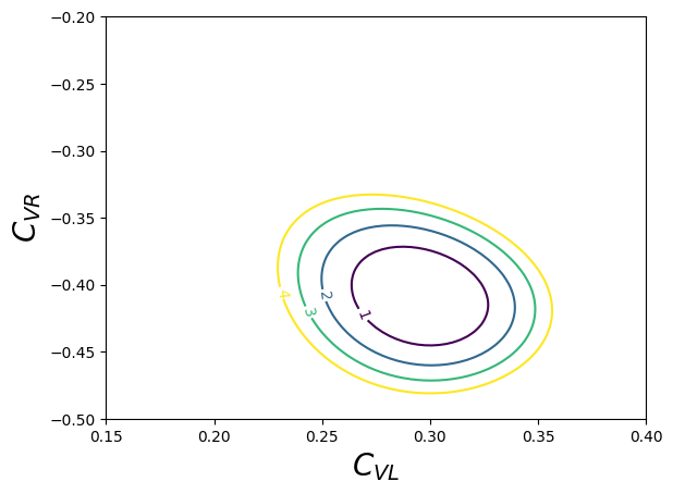
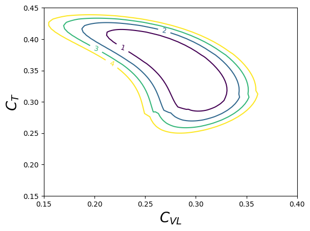
Figure 1: Fit to the WET parameters to the $R_{D^{*}}$ and $R_{J/\psi}$ ratios at $1\,\sigma$ (purple), $2\,\sigma$ (blue), $3\,\sigma$ (green) and $4\,\sigma$ (yellow).

In order to better understand the impact of NP on $R_{J/\psi}$ and its relation to $R_{D^{*}}$, we perform a statistical fit of the three Wilson coefficients in $C_{VR}$, $C_{VL}$ and $C_{T}$ including both observables. As mentioned before, the contribution of the scalar coefficients are negligible. The fit is performed by numerical minimization of the statistic test $\chi^{2}$ given by

$$\chi^{2}_{\mathrm{fit}}=\frac{1}{2}\sum_{i,j}[\mathcal{O}_{i}^{\mathrm{exp}}-\mathcal{O}_{i}^{\mathrm{th}}(\{C\})]\,\mathcal{C}_{ij}^{-1}\,[\mathcal{O}_{j}^{\mathrm{exp}}-\mathcal{O}_{j}^{\mathrm{th}}(\{C\})]\,,$$ (20)

where $\mathcal{O}_{i}^{\mathrm{exp}}$ and $\mathcal{O}_{i}^{\mathrm{th}}(\{C\})$ are the experimental measurement and theoretical prediction for the $i$-th observable, respectively, and $\mathcal{C}_{ij}$ is the correlation matrix. The result of the fit is represented in Fig. 1, by choosing two-dimensional contours of the Wilson coefficients with the rest of the parameters as fixed in the best fit point. The scalar contributions $C_{SL}$ and $C_{SR}$ are suppressed and the fit is constrained by the vector Wilson coefficients $C_{VL}$ and $C_{VR}$ and the tensor coefficient $C_{T}$. The values obtained for each coefficient are:

$$C_{VL} =0.296\pm 0.167\,, \quad C_{VR} =-0.409\pm 0.089\,, \quad C_{T} =0.341\pm 0.386\,.$$ (21)

The predictions for $R_{D},R_{D^{*}}$ and $R_{J/\psi}$ observables and their uncertainties in the best fit point are

$$R_{D}=0.342^{+0.039}_{-0.039}\,,\qquad R_{D^{*}}=0.288^{+0.022}_{-0.022}\,,\qquad R_{J/\psi}=0.345^{+0.026}_{-0.029}\,,$$ (22)

compatible with the experimental results within $1\,\sigma$.

2.2 $B\to K^{(*)}\nu\bar{\nu}$ decays

In the WET, the $B\to K^{(*)}\nu\bar{\nu}$ processes receive contributions from the effective operators appearing in the Lagrangian [29]

$$\mathcal{L}_{b\to s\nu\bar{\nu}}=-\frac{4G_{F}}{\sqrt{2}}\frac{\alpha_{\mathrm{em}}}{4\pi}\sum_{\nu,\nu^{\prime}}\left[(C_{L}^{\mathrm{NP}\,\nu\nu^{\prime}}+C_{L}^{\mathrm{SM}\,\nu\nu^{\prime}})\,O_{L}^{\nu\nu^{\prime}}+C_{R}^{\nu\nu^{\prime}}\,O_{R}^{\nu\nu^{\prime}}\right]+\mathrm{h.c.}\,,$$ (23)

where the semileptonic four-fermion operators are

$$O_{L}^{\nu\nu^{\prime}}=(\bar{s}\gamma_{\mu}P_{L}b)(\bar{\nu}\gamma^{\mu}P_{L}\nu^{\prime})\,,\qquad\qquad O_{R}^{\nu\nu^{\prime}}=(\bar{s}\gamma_{\mu}P_{R}b)(\bar{\nu}\gamma^{\mu}P_{L}\nu^{\prime})\,,$$ (24)

being $P_{R,L}=(1\pm\gamma_{5})/2$. The SM matching is $C_{L}^{\mathrm{SM}\,\nu\nu^{\prime}}=V_{tb}V_{ts}^{*}\,X_{\mathrm{SM}}\,\delta_{\nu\nu^{\prime}}$, where $V_{ij}$ are the elements of the CKM matrix, and $X_{\mathrm{SM}}=-12.64\pm 0.15$ [29, 52]. The branching ratios in the WET are calculated as

$$\mathrm{BR}(B^{+}\to K^{+}\nu\bar{\nu}) = A_{+}^{BK}\sum_{\nu,\nu^{\prime}}|(C_{L}^{\mathrm{NP}\,\nu\nu^{\prime}}+C_{L}^{\mathrm{SM}\,\nu\nu^{\prime}})+C_{R}^{\nu\nu^{\prime}}|^{2}\,,$$ (25)

$$\mathrm{BR}(B^{0}\to K^{*0}\nu\bar{\nu}) = A_{+}^{BK^{*}}\sum_{\nu,\nu^{\prime}}|(C_{L}^{\mathrm{NP}\,\nu\nu^{\prime}}+C_{L}^{\mathrm{SM}\,\nu\nu^{\prime}})+C_{R}^{\nu\nu^{\prime}}|^{2}$$ (26)

$$+ A_{-}^{BK^{*}}\sum_{\nu,\nu^{\prime}}|(C_{L}^{\mathrm{NP}\nu\nu^{\prime}}+C_{L}^{\mathrm{SM}\nu\nu^{\prime}})-C_{R}^{\nu\nu^{\prime}}|^{2}\,,$$

where $A_{+}^{BK}=(5.66\pm 0.17)\times 10^{-6}$ [29] and $A_{-}^{BK^{*}}=(8.88\pm 1.08)\times 10^{-6}$, $A_{+}^{BK^{*}}=(2.00\pm 0.29)\times 10^{-6}$ [31].

The tree-level match between the relevant SMEFT and the WET Wilson coefficients is [51]

$$C_{L}^{\mathrm{NP}\,\nu\nu^{\prime}} = -\frac{\sqrt{2}\pi}{G_{F}\Lambda^{2}\alpha_{\mathrm{em}}}\left(C_{\ell q(1)}^{\nu\nu^{\prime}23}-C_{\ell q(3)}^{\nu\nu^{\prime}23}+\delta_{\nu\nu^{\prime}}C_{\varphi q(1)}^{23}+\delta_{\nu\nu^{\prime}}C_{\varphi q(3)}^{23}\right)\,,$$

$$C_{R}^{\nu\nu^{\prime}} = -\frac{\sqrt{2}\pi}{G_{F}\Lambda^{2}\alpha_{\mathrm{em}}}\left(C_{\ell d}^{\nu\nu^{\prime}23}+\delta_{\nu\nu^{\prime}}C_{\varphi d}^{23}\right)\,.$$ (27)

Figure 2: Fit to the WET parameters affecting the $B\to K^{(*)}\nu\bar{\nu}$ branching ratios. The teal areas correspond to $\mathrm{BR}(B^{+}\to K^{+}\nu\bar{\nu})=(2.3\pm 0.7)\times 10^{-5}$ and the purple area to $\mathrm{BR}(B^{0}\to K^{*0}\nu\bar{\nu})<1.8\times 10^{-5}$, while the red areas are the best fit at $1\,\sigma$ and $2\,\sigma$.

When performing a fit that considers only the parameters $C_{L}^{33}$ and $C_{R}^{33}$ (third generation of neutrinos), we observe that the resulting values are located at the intersection between two parallel bands, which occur at $C_{L}^{33}+C_{R}^{33}=\mathrm{constant}$, consequence of the constraints imposed by the observable $B^{+}\rightarrow K^{+}\nu\bar{\nu}$; and the ellipse that corresponds to the constraints imposed by the observable $B^{0}\rightarrow K^{0*}\nu\bar{\nu}$ as shown in Figure 2. The two minima are located at

$$(C_{L}^{33},\,C_{R}^{33})=(-1.4\pm 0.6,\,-0.9\pm 0.6)\qquad\mathrm{and}\qquad(C_{L}^{33},\,C_{R}^{33})=(0.4\pm 0.6,\,0.9\pm 0.6)\,$$ (28)

and in both minima the predictions for the observables are

$$\mathrm{BR}(B^{+}\to K^{+}\nu\bar{\nu})=(2.2\pm 0.7)\times 10^{-5},\qquad\mathrm{BR}(B^{0}\to K^{*0}\nu\bar{\nu})=(1.3\pm 0.2)\times 10^{-5}\,,$$ (29)

compatible with the experimental measurements. We reproduce the results of [29] for their cLFC scenario. If only couplings to left-handed quarks are allowed, the best fits are obtained for $C_{L}^{33}=0.9\pm 0.3$ or $-2.0\pm 0.3$, corresponding to $\mathrm{BR}(B^{+}\to K^{+}\nu\bar{\nu})=(1.5\pm 0.6)\times 10^{-5}$ and $\mathrm{BR}(B^{0}\to K^{*0}\nu\bar{\nu})=(1.8\pm 1.0)\times 10^{-5}$. Therefore, we can conclude that $C_{L}^{33}$ alone can reduce the tension to the $1\,\sigma$ level, while the addition of $C_{R}^{33}$ is necessary to fully describe the experimental data.

3 Global fits

In this section we will update and extend the results obtained in [1], which used a subset of the SMEFT operators first proposed by [53, 54, 55]. The dimension-6 Lagrangian in the “Warsaw-down” basis takes the form [1]

$$\mathcal{L}_{\mathrm{NP}}=\frac{\lambda^{\ell}_{ij}\lambda^{q}_{kl}}{\Lambda^{2}}[C_{1}(\bar{\ell}_{i}\gamma_{\mu}\ell_{j})(\bar{q}_{k}\gamma^{\mu}q_{\ell})+C_{3}(\bar{\ell}_{i}\gamma_{\mu}\tau^{I}\ell_{j})(\bar{q}_{k}\gamma^{\mu}\tau^{I}q_{\ell})]\,,$$ (30)

where $\ell_{i}$ and $q_{i}$ are the $SU(2)_{L}$ doublets for the $i$-th generation of leptons and quarks, respectively, $\Lambda$ is the energy scale where the UV theory is matched to the SMEFT, $C_{1}$ and $C_{3}$ are the Wilson coefficients for singlet and triplet interactions, with the identification $C_{\ell q(1)}^{ijkl}=C_{1}\lambda^{\ell}_{ij}\lambda^{q}_{kl}$ and $C_{\ell q(3)}^{ijkl}=C_{3}\lambda^{\ell}_{ij}\lambda^{q}_{kl}$, being $\lambda^{\ell}$ and $\lambda^{q}$ the matrices that determine the flavour structure of the NP interactions. We will fix the value $\Lambda=1\,\mathrm{TeV}$, which assumes that the NP effects can be observed in flavour physics experiments. Flavour-changing charged currents can only be mediated by triplet interactions, and therefore $C_{3}$ is necessary to describe the $R_{D^{(*)}}$ and $R_{J/\psi}$ anomalies. Flavour-changing neutral currents, on the other hand, are mediated by both $C_{1}$ and $C_{3}$, in particular the contributions to $b\to s\ell^{+}\ell^{-}$ are proportional to $C_{1}+C_{3}$, while $b\to s\nu\bar{\nu}$ receives tree-level contributions from $C_{1}-C_{3}$. Finally, the matrices $\lambda$ are a reflection of the flavour structure of the UV theory. One simple case, proposed by [53], considered that the UV theory only affected one generation of fermions in a certain interaction basis, which needs to be rotated to the mass basis. In this case, the matrices must be hermitian, idempotent ($\lambda^{2}=\lambda$) and $\mathrm{tr}\,\lambda=1$ and, as explained in [1], can be parameterized by two complex numbers, $\alpha^{\ell,q}$ and $\beta^{\ell,q}$, in the following way:

$$\lambda^{\ell,q}=\frac{1}{1+|\alpha^{\ell,q}|^{2}+|\beta^{\ell,q}|^{2}}\begin{pmatrix}|\alpha^{\ell,q}|^{2}&\alpha^{\ell,q}\bar{\beta}^{\ell,q}&\alpha^{\ell,q}\\ \bar{\alpha}^{\ell,q}\beta^{\ell,q}&|\beta^{\ell,q}|^{2}&\beta^{\ell,q}\\ \bar{\alpha}^{\ell,q}&\bar{\beta}^{\ell,q}&1\end{pmatrix}\,.$$ (31)

In order to be consistent in our analysis, we must not restrict ourselves to the ratios $R_{D^{(*)}}$ and $R_{J/\psi}$. The first reason is that the Langrangian (30) directly contributes to many other physical observables, for example the previously mentioned $\mathrm{BR}(B\to K^{(*)}\nu\bar{\nu})$ and even Lepton Flavour violating processes, like $B\to Ke^{\pm}\mu^{\mp}$, due to the off-diagonal terms of $\lambda^{\ell}$. In addition, the running of the Renormalization Group equations causes the mixing of the operators in Lagrangian (30) with other SMEFT operators. For example, the insertion of $O_{\ell q(1)}$ ($O_{\ell q(3)}$) is necessary for the one loop corrections to $O_{\varphi q(1)}$ and $O_{\varphi\ell(1)}$ ($O_{\varphi q(3)}$ and $O_{\varphi\ell(3)}$) operators that are relevant for interactions between $Z$ bosons and fermions. This justifies the need to perform global fits including various observables from $B$-physics and electroweak precision tests.

	Scenario I	Scenario II	Scenario III
$C_{1}$	$-0.11^{+0.03}_{-0.04}$	$-0.12\pm 0.03$	$-0.205\pm 0.015$
$C_{3}$	$-0.11^{+0.03}_{-0.04}$	$-0.12\pm 0.03$	$-0.12^{+0.02}_{-0.01}$
$\alpha^{\ell}$	–	$0.0\pm 0.07$	–
$\beta^{\ell}$	$0.00\pm 0.02$	$0.000\pm 0.014$	–
$\alpha^{q}$	–	$-0.076$	–
$\beta^{q}$	$0.78^{+1.22}_{-0.36}$	$0.85^{+1.05}_{-0.6}$	$0.64^{+1.36}_{-0.24}$
Pull	$5.71\,\sigma$	$5.51\,\sigma$	$6.25\,\sigma$
$\Delta\chi^{2}_{\mathrm{SM}}$	39.8	43.12	46.66
$p$-value	$1.2\times 10^{-8}$	$3.5\times 10^{-8}$	$4.1\times 10^{-10}$

Table 1: Results of the best fits to the rotation parameters and the coefficients $C$ in Scenario I, II and III.

We have performed the fits including all observables implemented by smelli version 2.3.3 [56] plus $R_{J/\psi}$. The goodness of each fit is evaluated with its difference of $\chi^{2}$ with respect to the SM, $\Delta\chi^{2}_{\mathrm{SM}}=\chi^{2}_{\mathrm{SM}}-\chi^{2}_{\mathrm{fit}}$, being $\chi^{2}_{\mathrm{fit}}$ as defined in (20). Besides, the package smelli computes the differences of the logarithms of the likelihood function as $\Delta\log L=-\frac{1}{2}\Delta\chi^{2}_{\mathrm{SM}}$ and, in order to compare two fits $A$ and $B$, we use the pull between them in units of $\sigma$, defined as [57]

$$\mathrm{Pull}_{A\to B}=\sqrt{2}\mathrm{Erf}^{-1}[F(\Delta\chi^{2}_{A}-\Delta\chi^{2}_{B};n_{B}-n_{A})]\,,$$ (32)

where $\mathrm{Erf}^{-1}$ is the inverse of the error function, $F$ is the cumulative distribution function of the $\chi^{2}$ distribution and $n$ is the number of degrees of freedom of each fit. The SM input parameters are chosen to be the same as in our previous work [1].

For comparison with our previous results, we have considered the two scenarios defined in [1] and, motivated by the tension in the new $B^{+}\to K^{+}\nu\bar{\nu}$ measurement at Belle II [28] together with the alleviation of the tension in the $R_{K^{(*)}}$ ratios, we have introduced a new scenario called Scenario III:

• Scenario I: Includes only mixing between the second and third generations through $\beta^{\ell}$ and $\beta^{q}$, that is, $\alpha^{\ell}=\alpha^{q}=0$ and $C_{1}=C_{3}\equiv C$.

• Scenario II: The only assumption is $C_{1}=C_{3}\equiv C$. Mixing with both first and second generation leptons through $\alpha^{\ell}$, $\beta^{\ell}$, $\alpha^{q}$ and $\beta^{q}$ is considered.

• Scenario III: $C_{1}$ and $C_{3}$ are independent parameters, and we do not consider mixing in the lepton sector, that is $\alpha^{\ell}=\beta^{\ell}=0$.

Scenarios I and II assumed that $C_{1}=C_{3}\equiv C$ because at that time, the $R_{K^{(*)}}$ observables presented deviations as compared to their SM predictions, while the constraints set by the $B\to K^{(*)}\nu\bar{\nu}$ decays were quite stringent. However, at present the experimental situation has reversed, with the tension in the $R_{K^{(*)}}$ ratios disappearing and a new anomaly appearing in $B^{+}\to K^{+}\nu\bar{\nu}$, pointing towards different NP contributions to $C_{1}$ and $C_{3}$. Scenario III assumes that $C_{1}$ and $C_{3}$ are independent parameters and. Additionally, since there are no longer discrepancies in muonic observables, we do not consider mixing in the lepton sector ($\alpha^{\ell}=\beta^{\ell}=0$); we are also discarding mixing to the first quark generation since it played no role in our previous fits. In all three scenarios, only real values for the fit parameters are considered.

The results of the best fits to the rotation parameters and the coefficients $C$ are summarized in Table 1. Scenarios I and II present a similar best fit point, with $C\sim-0.12$, $\beta^{q}=0.8$ and the rest of the rotation parameters compatible with zero. The $\Delta\chi^{2}_{\mathrm{SM}}$ is also similar, with $\Delta\chi^{2}_{\mathrm{SM}}=39.8$ in Scenario I and $\Delta\chi^{2}_{\mathrm{SM}}=43.1$ in Scenario II, which results in Scenario I having a better pull because there are less degrees of freedom, i.e. it is a simpler hypothesis. As anticipated, Scenario III results in a much better fit as compared to Scenarios I and II, since it requires the minimum number of parameters needed to describe simultaneously the anomalies in $R_{D^{(*)}}$ and $B\to K\nu\bar{\nu}$, with $\Delta\chi^{2}_{\mathrm{SM}}=46.66$ and a pull of $6.25\,\sigma$.

In Scenario III, since $\alpha^{\ell}=\beta^{\ell}=0$, there is no mixing in the leptonic sector, and the NP only affects the third generation, i.e., $\lambda^{\ell}_{33}=1$ and $\lambda^{\ell}_{ij}=0$ for all the other entries. Meanwhile, with a fit value of $\beta^{q}$ close to one, there is a large mixing between the second and third quark generations, resulting in $\lambda^{q}_{22}=0.29$, $\lambda^{q}_{33}=0.71$ and $\lambda^{q}_{23}=\lambda^{q}_{32}=0.45$. This mixing structure thus provides large contributions to $b\to s\,\nu_{\tau}\bar{\nu}_{\tau}$ and $b\to c\,\tau^{-}\bar{\nu}_{\tau}$ transitions while leaving $b\to s\,e^{+}e^{-}$ and $b\to s\,\mu^{+}\mu^{-}$ unaltered at tree level.

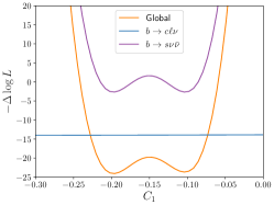
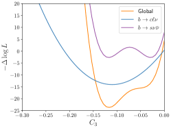
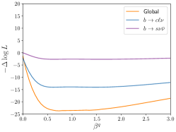
(a)	(b)	(c)

Figure 3: Negative of the logarithm of the likelihood function when varying (a) $C_{1}$ (b) $C_{3}$ and (c) $\beta^{q}$ with respect to their values at the best fit for Scenario III.

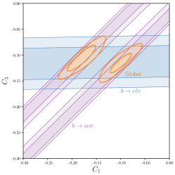
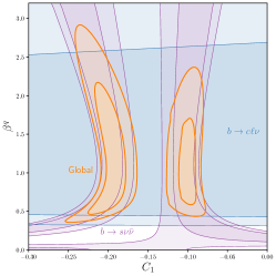
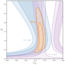
(a)	(b)	(c)

Figure 4: Regions of constant likelihood in Scenario III for (a) $C_{1}$ and $C_{3}$ plane (b) $C_{1}$ and $\beta^{q}$ plane and (c) $C_{3}$ and $\beta^{q}$ plane, with the rest of parameters as in the best fit point of Scenario III.

The role of each parameter of the fit in constraining each class of observables is shown in Figures 3 and 4. The one-dimensional slices of the likelihood function for Scenario III is included in Fig. 3. The global fit (in orange) consists of 593 observables listed in Appendix A. However, it can be seen that it is largely dominated by the two classes of observables that we have been discussing in the previous sections: $b\to c\ell\nu$ (in blue) and $b\to s\nu\bar{\nu}$ (in purple). In particular, the $b\to s\nu\bar{\nu}$ observables determine the likelihood function in the direction of the parameter $C_{1}$, both $b\to c\ell\nu$ and $b\to s\nu\bar{\nu}$ contribute to the likelihood function in the direction of $C_{3}$, and $b\to c\ell\nu$ observables present the most important contribution to the likelihood in the direction of $\beta^{q}$. A similar picture emerges in Fig. 4 when the contours of constant likelihood are considered. As indicated by the matching conditions in Eqs (19) and (27), the Wilson coefficient $C_{VL}$ relevant for the $b\to c\ell\nu$ decays depends on $C_{\ell q(3)}^{3323}=C_{3}\lambda^{q}_{23}$ while the coefficient $C_{L}^{33}$ of the $b\to s\nu\bar{\nu}$ observables depends on both $C_{\ell q(1)}^{3323}=C_{1}\lambda^{q}_{23}$ and $C_{\ell q(3)}^{3323}=C_{3}\lambda^{q}_{23}$.

After applying the running of the Renormalization Group equation and the matching conditions (see [1] for details), the Wilson coefficients relevant for the $b\to c\,\tau^{-}\bar{\nu}_{\tau}$ and $b\to s\,\nu_{\tau}\bar{\nu}_{\tau}$ processes at the scale $\mu=m_{b}$ are

$$C_{VL}=0.089\,,\qquad\qquad C_{L}^{33}=0.61\,,$$ (33)

while the other coefficients in Eq. (19) and Eq. (27) do not receive contributions from Scenario III. There is also a contribution to the Wilson coefficient $C_{9}^{\ell}$ which enters the $b\to s\,\ell^{+}\ell^{-}$ decays for $\ell=e,\,\mu$ [1]. Since this contribution is generated radiatively from $C_{9}^{\tau}$, it is lepton flavour universal for the light flavours, $C_{9}^{e}=C_{9}^{\mu}=-0.58$, and consequently it does not affect the $R_{K^{(*)}}$ ratios, which remain at their SM values $R_{K^{(*)}}\approx 1$. However, this contribution does enter in the branching ratios of $B\to K^{(*)}\mu^{+}\mu^{-}$ and $B_{s}\to\phi\,\mu^{+}\mu^{-}$.

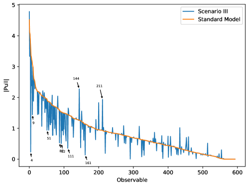
Figure 5: Pull of the observables considered for the global fit in the SM (orange line) and Scenario III (blue line). The observables are ordered by decreasing SM pull, and the ones in which the SM and Scenario III differ more than $1\,\sigma$ are specially marked.

The predictions for all the observables included in the fit, as well as the pull in the SM and in Scenario III (NP pull), are given in Appendix A. Fig. 5 shows the comparison of the pull of each observable with respect to their experimental value in the SM (orange line) and in the Scenario III (blue line). Here the observables in which the SM and Scenario III differ more than $1\,\sigma$ are highlighted. We observe that the highlighted observables are all related to the $B$-meson anomalies: $R_{D^{*}}^{\ell}$ (observable 4) and $R_{D}^{\ell}$ (observable 92) improve by $3.3\,\sigma$ and $1\,\sigma$ respectively; $\mathrm{BR}(B^{+}\to K^{+}\nu\bar{\nu})$ (observable 9) improves by $1.7\,\sigma$ and $\mathrm{BR}(B^{+}\to K^{*+}\nu\bar{\nu})$ (observable 161) by $1\,\sigma$ while $\mathrm{BR}(B^{0}\to K^{*0}\nu\bar{\nu})$ (observable 144) gets worse by $1\,\sigma$. And finally, regarding the branching ratios of $b\to s\mu^{+}\mu^{-}$ at high $q^{2}$, $\mathrm{BR}(B^{\pm}\to K^{\pm}\mu^{+}\mu^{-})$ in the $[16-17]\,\mathrm{GeV}^{2}$ (observable 51) and $[15-22]\,\mathrm{GeV}^{2}$ (observable 87) bins, as well as $\mathrm{BR}(B_{s}^{\pm}\to\phi^{\pm}\mu^{+}\mu^{-})$ in the $[15-19]\,\mathrm{GeV}^{2}$ bin (observable 111), improve by around $1\,\sigma$ while $\mathrm{BR}(B^{\pm}\to K^{\pm}\mu^{+}\mu^{-})$ in the $[17-18]\,\mathrm{GeV}^{2}$ bin (observable 211) gets worse also by $1\,\sigma$. As pointed out in Section 2.2, it is not possible to describe $B^{+}\to K^{+}\nu\bar{\nu}$ and $B^{0}\to K^{*0}\nu\bar{\nu}$ decays only with left-handed effective operators, consequently resulting in a worse pull for observable 144. As for the $B^{+}\to K^{+}\mu^{+}\mu^{-}$ differential branching ratios, both LHCb [2] and CMS [19] find some tension between the $[17-18]\,\mathrm{GeV}^{2}$ bin, which is measured above the SM prediction, and the rest of the bins in the $q^{2}\geq 15\,\mathrm{GeV}^{2}$, which are below their SM prediction, and our fit reproduces said tension.

3.1 Comparison with previous results

The inclusion of the new experimental measurements at LHCb for $R_{K^{(*)}}$ [43, 58] has significantly impacted our global fit, as compared to previous results presented in [1]. In the previous fit, we found that a sizable contribution to $\alpha^{\ell}$ was needed to describe the $R_{K^{(*)}}$ anomaly via NP affecting the electron decay mode. Now that the experimental measurements for $R_{K^{(*)}}$ are compatible with the SM predictions, the current fit no longer requires large deviations in $\alpha^{\ell}$. In consequence, there is no mixing in the leptonic sector, with $\lambda^{\ell}_{33}\approx 1$ affecting the tau decays (required to describe LFUV in $b\to c\tau\nu_{\tau}$ processes), while $\lambda^{\ell}_{ij}\approx 0$ for $ij\neq 33$. In the quark sector, the central values found by the fit present no significant changes as compared to the previous one, with large NP effects in $\beta^{q}$ needed to describe the anomalies in flavour-changing $b\to c$ charged currents. However, we observe that $\beta^{q}$ presents a larger allowed range, including even regions with $\beta^{q}>1$, that is, with larger NP effects in the second generation than in the third generation. In the previous fit, $\beta^{q}$ was constrained by the LFV decays $B\to K^{(*)}\mu e$, which received NP contributions through $C\lambda^{q}_{23}\lambda^{\ell}_{12}\sim C\beta^{q}\alpha^{\ell}\beta^{\ell}$. With the new fit preferring values of $\alpha^{\ell}$ much closer to zero, the impact of $\beta^{q}$ in the LFV observables is decreased, and instead, $\beta^{q}$ is controlled mainly by the $b\to c\ell\nu$ decays.

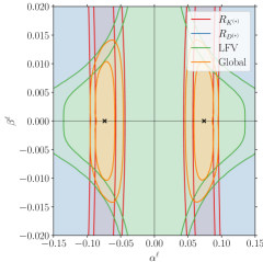
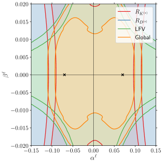
(a)	(b)

Figure 6: Regions of constant likelihood for $\alpha^{\ell}$ and $\beta^{\ell}$ parameters in Scenario II as (a) in the previous work [1] and (b) in the current work.

This is illustrated in Figure 6, where the two-dimensional section of the likelihood function for the parameters $\alpha^{\ell}$-$\beta^{\ell}$ in Scenario II, with the rest of the parameters set at the best fit point of this scenario, is compared between the previous fit (left) and the new fit (right). In [1] we found that the better fit, with the inclusion of previous discrepancies on $R_{K}$ and $R_{K^{*}}$ results, corresponded to Scenario II. However, the present experimental measurements of these ratios do not have discrepancies with the SM predictions anymore. In fact, it can be seen that the main difference is the region allowed for the $R_{K^{(*)}}$ observables, inside the red lines: in the previous fit, the allowed region corresponded to $0.04\leq|\alpha^{\ell}|\leq 0.10$, which was not compatible with the SM value $\alpha^{\ell}=0$ owing to the experimental anomalies at that moment. On the other hand, the allowed region in the current fit is $0\leq|\alpha^{\ell}|\leq 0.12$, which includes the SM point since the anomalies are gone. The global fit, in orange, follows the same logic.

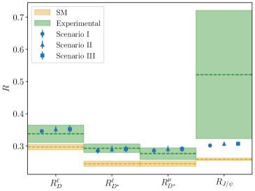
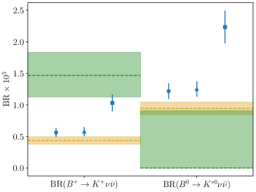
(a)	(b)

Figure 7: Predictions for selected (a) $b\to c\ell\nu$ LFU ratios and (b) $b\to s\nu\bar{\nu}$ branching ratios. The predictions in Scenarios I, II and III and their expected error are represented with blue markers. The SM prediction and its $1\,\sigma$ error are represented by the yellow regions. The experimental measurement and its $1\,\sigma$ error are represented by the green regions.

The predictions for $R_{D}$, $R_{D^{*}}$ and $R_{J/\psi}$ observables in the best fit points for Scenarios I, II and III are shown in Figure 7(a). $R_{D}$ and $R_{D^{*}}$ exhibit very similar values in both scenarios II and III (as $\alpha^{l,q}$ does not affect these predictions), and these fitted values align well with experimental results. The current fit is largely dominated in the $b\to c\ell\nu$ sector by the $R_{D^{(*)}}$ ratios, as their uncertainty is much smaller than in the case of $R_{J/\psi}$. It would be therefore desirable to improve the measurements of $R_{J/\psi}$ in order to obtain an independent handle of the $b\to c\ell\nu$ sector and further clarify the present anomaly.

Figure 7(b) includes the predictions for $B^{+}\to K^{+}\nu\bar{\nu}$ and $B^{0}\to K^{*0}\nu\bar{\nu}$ branching ratios. In both cases we can see how the scenario I and II, in which the coefficients $C_{1}=C_{3}$ were not independent, fail to correctly capture the NP contribution, yielding values very close to the SM predictions. In contrast, Scenario III manages to improve the results in the charged sector, although the results in the neutral sector are worsened.

Observable	Previous fit	Current fit
$R_{K}^{[1.1,\ 6.0]}$	0.83 ($0.28\,\sigma$)	1.001 ($1.1\,\sigma$)
$R_{K^{*0}}^{[0.045,1.1]}$	0.884 ($2.1\,\sigma$)	0.924 ($0.026\,\sigma$)
$R_{K^{*0}}^{[1.1,6.0]}$	0.84 ($1.4\,\sigma$)	0.996 ($0.41\,\sigma$)
$R_{D}^{\ell}$	0.351 ($0.16\,\sigma$)	0.344 ($0.51\,\sigma$)
$R_{D^{*}}^{\ell}$	0.290 ($0.41\,\sigma)$	0.283 ($0.23\,\sigma)$
$R_{D^{*}}^{\mu}$	0.290 ($0.75\,\sigma)$	0.284 ($0.77\,\sigma)$
$R_{J/\psi}$	-	0.306 ($1.1\,\sigma)$
$\mathrm{BR}(B^{+}\to K^{+}\nu\bar{\nu})$	$0.577\times 10^{-5}$ ($1.1\,\sigma$)	$0.970\times 10^{-5}$ ($1.4\,\sigma$)
$\mathrm{BR}(B^{0}\to K^{*0}\nu\bar{\nu})$	$1.252\times 10^{-5}$ ($1.5\,\sigma$)	$2.104\times 10^{-5}$ ($2.3\,\sigma$)

Table 2: Comparison of the predictions for $b\to s\ell^{+}\ell^{-}$, $b\to c\ell\nu$ and $b\to s\nu\bar{\nu}$ observables between our previous fit and the current fit in Scenario II. The significance of the predictions in the column “Previous fit” are referred to the experimental measurements that were available in Ref. [1], while the significances in the column “Current fit” correspond to the updated values.

The comparison of the values obtained for $b\to s\ell^{+}\ell^{-}$, $b\to c\ell\nu$ and $b\to s\nu\bar{\nu}$ observables analyzed in this paper can be found in Table 2. The significance of the deviations with respect to the experimental values, in units of $\sigma$, is included for all observables. The ones in the column “Previous fit” are referred to the experimental measurements that were available in Ref. [1], while the ones in the column “Current fit” correspond to the updated values in this work. In the case of the $R_{K^{(*)}}$ ratios, the current fit improves the pull for $R_{K^{*0}}^{[1.1,6.0]}$ and $R_{K^{*0}}^{[0.045,1.1]}$, the later by almost $2\,\sigma$. At the same time, the pull for $R_{K^{+}}^{[1.1,\ 6.0]}$ has increased to $1.1\,\sigma$. The reason for this change is that this is the only bin where some of the tension with the SM prediction still survives, and our fit reproduces this tension. The updated measurements of $R_{D^{(*)}}$ and the inclusion of the observable $R_{J/\psi}$ with its large uncertainty, have a lesser impact on our fit. However, for the $R_{D^{(*)}}$ ratio that includes the decay mode to electrons, $R_{D^{*}}^{\ell}$, this work marks an improvement over the previous fit due to the reduced NP effects in $\alpha^{\ell}$.

The impact of the new measurement and the reduced NP effects in $\alpha^{\ell}$ can also be noticed in other $b\to se^{+}e^{-}$ observables, for example in the inclusive branching ratio $\mathrm{BR}(B\to X_{s}\,e^{+}e^{-})$, that has changed from $1.3\,\sigma$ to $1.6\,\sigma$ in the $[14.2,\,25.0]\,\mathrm{GeV}^{2}$ bin (observable 113 in Appendix A) and from $0.23\,\sigma$ to $0.74\,\sigma$ in the $[1.0,\,6.0]\,\mathrm{GeV}^{2}$ bin (observable 407). Also in LFU ratios, like other bins of $R_{K^{(*)}}$ that were measured by Belle [59], for example $R_{K^{0}}^{[4.0,\,8.12]}$ changing from $0.86\,\sigma$ to $1.3\,\sigma$ (observable 140) and $R_{K^{+}}^{[4.0,\,8.12]}$ from $1\,\sigma$ to $0.59\,\sigma$ (observable 343). By contrast, $b\to s\mu^{+}\mu^{-}$ observables like the angular observables ${P^{\prime}}_{4}$ and ${P^{\prime}}_{5}$ or the branching ratios $\mathrm{BR}(B\to K^{*}\mu^{+}\mu^{-})$ and $\mathrm{BR}(B_{s}\to\phi\,\mu^{+}\mu^{-})$ remain unchanged between both fits, because the value for $\beta^{\ell}$ has not changed.

3.2 Machine Learning analysis

In this section we summarize some details of the Machine Learning (ML) algorithm used in this work, by following the procedure explained in [1]. Since the obtained likelihood contours do not adhere to a Gaussian distribution, the ML algorithm is used to generate samples that match the obtained distributions. Besides, we use a Montecarlo analysis using Machine Learning to extract the confidence intervals and correlations between observables, as given in [1].

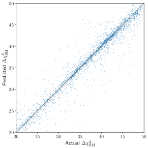
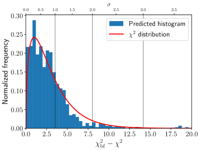
(a)	(b)

Figure 8: (a) Linear regression between the actual values of the $\Delta\chi^{2}_{\mathrm{bf}}$ (horizontal axis) and the values predicted by the XGBoost model (vertical axis) in the validation set in Scenario III. (b) Histogram of the sample of points generated by the Machine Learning-based Monte Carlo algorithm in Scenario III, in blue, compared to the $\chi^{2}$ probability distribution function, in red.

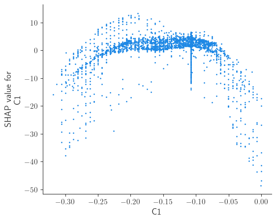
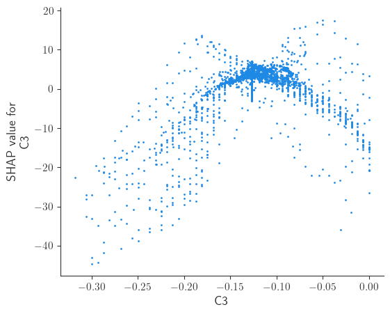
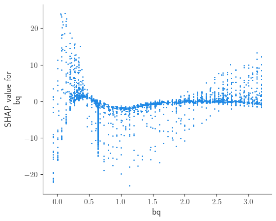
(a)	(b)	(c)

Figure 9: Distribution of SHAP values for each parameter of the fit: (a) $C_{1}$, (b) $C_{3}$, (c) $\beta^{q}$.

Using the XGBoost (eXtreme Gradient Boosting) algorithm we can train an ensemble of regression trees capable of approximating the log-likelihood function of our fit. We built a training sample of 5,000 parameter points with their corresponding likelihood values and split it into two parts: $50\%$ of the points for training and $50\%$ of the points for validation of the model. We train the ML model with a learning rate of $0.03$ and allow early stopping after 5 rounds of stagnant learning. The training process finalized after 860 boosting rounds.

The correlation between the actual values of the $\chi^{2}_{\mathrm{SM}}$ in the validation dataset and the corresponding predictions by the ML model is included in Figure 8(a) for Scenario III. The Pearson coefficient for linear correlation is $r=0.96$, indicating an excellent agreement. The histogram for the predicted $\chi^{2}$ values in Figure 8(b) shows how, once again, the ML-generated points closely follow the general shape of the $\chi^{2}$ distribution.

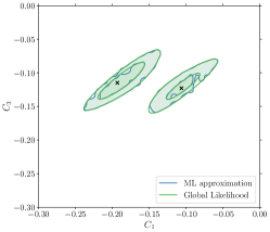
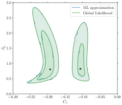
(a)	(b)	(c)

Figure 10: Comparison between the $1\,\sigma$ and $2\,\sigma$ likelihood contours obtained using the ML approximation (blue) and the actual contours (green) in (a) $C_{1}$ and $C_{3}$ plane, (b) $C_{1}$ and $\beta^{q}$ plane and (c) $C_{3}$ and $\beta^{q}$ plane.

After training the model and generating a sample of points using a Machine Learning Montecarlo algorithm, we plotted the logarithm of the likelihood while varying different parameters, as shown in Figure 9. Note that the parameters follow the shapes obtained in the global fit as presented in Figure 3 (with negative sign). The columns of dots visible in the three plots result from an overrepresentation of the best-fit points in the data sets for $C_{1}=-0.11$, $C_{3}=-0.12$ or $\beta^{q}=0.6$. This effect arises from using a combination of two different data sets: one with randomly generated points across the parameter space, and another with points in a grid used for the elaboration of Fig. 4. In the latter, each pair of parameters is sampled while keeping the remaining parameter fixed at its best-fit value. We also obtained the contours depicted in Figure 10, showing a high degree of agreement with the contours obtained in the fit. Therefore, we can conclude that ML, made jointly with the SHAP values, reproduce correctly the general features of the fit and it’s a suitable strategy for this kind of analysis.

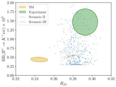
Figure 11: Values of the observables $R_{D^{*}}$ and $\mathrm{BR}(B^{+}\to K^{+}\nu\bar{\nu})$ in the ML-generated samples for scenario II (orange points) and scenario III (blue points), compared to the SM prediction (yellow region) and experimental measurement (green region).

Finally, it is worth mentioning that in [1] we determined the predictions of our model for several selected observables of various flavour sectors, including the $R_{D^{*}}$ observables and $B^{+}\to K^{+}\nu\bar{\nu}$ decay. The results showed an almost-perfect correlation for these two observables. The predictions for these two observables in the generated sample were shown in Figure 12 of [1]. With the inclusion of the new experimental results on $R_{D^{*}}$ ratios at Belle II [17] and our new Scenario III, in which the Wilson coefficients $C_{1}$ and $C_{3}$ are independent parameters and not mixing in the lepton sector is considered, our previous results change drastically. Predictions for these two observables in the ML-generated samples for Scenario II (as in the previous paper) and Scenario III are shown in Figure 11, where we can observe how the correlation present in Scenario II dissappears in Scenario III. Building a UV complete model reproducing the interplay between $R_{D^{*}}$ and $\mathrm{BR}(B^{+}\to K^{+}\nu\bar{\nu})$ in Fig. 11 is out of the scope of this work. However there are some proposals in the literature that describe the $R_{D^{(*)}}$ anomalies while enhancing $\mathrm{BR}(B^{+}\to K^{+}\nu\bar{\nu})$ with vector leptoquarks [60, 61], non-universal $Z^{\prime}$ bosons [62] or combinations of scalars and fermions [63].

4 Conclusions

In this paper we have performed an improved analysis of the anomalies in $B$-meson decays by using an effective field theory approach and considering the NP effects on the Wilson coefficients of the effective Lagrangian. This work is based on results from our previous work [1] in which a global fit to experimental data available at that time was performed, with the inclusion of anomalies on the ratios of branching fractions for the $b\to s\ell^{+}\ell^{-}$ processes, $R_{K}$ and $R_{K^{*}}$. In view of the latest experimental results of $R_{K}$ ratios and the new deviation observed on $B^{+}\to K^{+}\nu\bar{\nu}$ decay at Belle II, an updated global fit is recommended. Consequently, a new scenario (Scenario III) is considered in the present study, with only mixing between the second and third quark generations and no mixing in the lepton sector, being the Wilson coefficients for the singlet and triplet four fermion effective operators independent. Both the recent experimental measurements of $\mathrm{BR}(B^{+}\rightarrow K^{+}\nu\bar{\nu})$ and $R_{J/\psi}$ are included in the present analysis. Besides, branching ratios associated with $B\rightarrow D^{(*)}\tau\nu$ decays are considered. The fact that the global fit is dominated by these classes of observables underlines their potential as probes to NP. All these ingredients have led to a marked improvement in our results compared to the previous study.

We use a Machine Learning (ML) algorithm in our analysis, by checking the agreement between the results obtained for this procedure and both the general shape of the $\Delta\chi^{2}$ distribution and the analysis of the impact of each parameter on the global fit. In our Scenario III, the $B\to K^{(*)}\nu\bar{\nu}$ observables constrain the parameter $C_{1}$, both $B\to D^{(*)}\ell\nu$ and $B\to K^{(*)}\nu\bar{\nu}$ constrain $C_{3}$, and $B\to D^{(*)}\ell\nu$ observables present the most important constraint to $\beta^{q}$.

The results of the global fit after including a wide range of flavour and electroweak observables are displayed in Table 1, and the predictions for the most relevant observables are summarized in Table 2. The comparison with the previous scenarios considered in [1] is included in the discussion. Our results show that Scenario III, which introduces independent parameters $C_{1}$ and $C_{3}$ without mixing in the lepton sector, provides the best fit to experimental results, achieving a pull of $6.25\,\sigma$. This scenario successfully accounts for the discrepancies observed in $R_{D^{*}}$ and $R_{J/\psi}$ measurements while maintaining consistency with the Standard Model in the $R_{K}$ ratios. Furthermore, it improves the predicted branching ratio for $\mathrm{BR}(B^{+}\rightarrow K^{+}\nu\bar{\nu})$ although it does not fully explain $\mathrm{BR}(B^{0}\rightarrow K^{*0}\nu\bar{\nu})$. The results are pointing in the direction of NP that interacts mainly with the third generation of leptons, reminiscent of the $U(2)$ flavour symmetry hypothesis [64, 65]. The situation would be clarified further with measurements of $R_{J/\psi}$ achieving a resolution similar to that of $R_{D^{(*)}}$, and with additional $\tau$ observables, for example the longitudinal polarisation in $B_{c}\to J/\psi\tau\nu$ or the branching ratio of $B\to K^{(*)}\tau^{+}\tau^{-}$.

Appendix A Pulls of the observables

The list of all observables that contribute to the global fit, as well as their prediction in Scenario III and their pull in both scenario III (NP pull) and SM is collected in this appendix. Observables are ordered according to their SM pull, and color-coded according to the difference between the scenario III and SM pulls, such that the observables with a better pull in scenario III are in green and red observables have a better pull in the SM.

Predictions for dimensionful observables are expressed in the corresponding power of GeV. The notation $\langle\cdot\cdot\cdot\rangle$ means that the observable is binned in the invariant mass-squared of the di-lepton system $q^{2}$, with the endpoints of the bin in $\mathrm{GeV}^{2}$ given in the superscript. Accordingly, the notation $\frac{\langle\mathrm{BR}\rangle}{\mathrm{BR}}$ denotes a binned branching ratio normalised to the total branching ratio.

	Observable	NP prediction	NP pull	SM pull
0	$\langle\frac{d\mathrm{BR}}{dq^{2}}\rangle(B^{\pm}\to K^{\pm}\mu^{+}\mu^{-})^{[19.24,\ 22.9]}$	$5.5449\times 10^{-9}$	4.8 $\sigma$	4.5 $\sigma$
1	$\langle\frac{d\overline{\mathrm{BR}}}{dq^{2}}\rangle(B_{s}\to\phi\mu^{+}\mu^{-})^{[2.5,\ 4.0]}$	$4.6141\times 10^{-8}$	3.3 $\sigma$	4.1 $\sigma$
2	$\langle\mathrm{BR}\rangle(D^{0}\to\pi^{-}e^{+}\nu_{e})^{[2,\ 2.98]}$	0.00022544	4.1 $\sigma$	4.1 $\sigma$
3	$a_{\mu}$	0.0011659	3.8 $\sigma$	3.8 $\sigma$
4	$R_{\tau\ell}(B\to D^{\ast}\ell^{+}\nu)$	0.28951	0.23 $\sigma$	3.6 $\sigma$
5	$\langle P_{2}\rangle(B^{0}\to K^{\ast 0}\mu^{+}\mu^{-})^{[0.1,\ 0.98]}$	-0.13043	3.3 $\sigma$	3.4 $\sigma$
6	$\langle F_{L}\rangle(B^{+}\to K^{\ast+}\mu^{+}\mu^{-})^{[2.5,\ 4]}$	0.77432	3.2 $\sigma$	3.3 $\sigma$
7	$\langle\frac{d\overline{\mathrm{BR}}}{dq^{2}}\rangle(B_{s}\to\phi\mu^{+}\mu^{-})^{[4.0,\ 6.0]}$	$4.8791\times 10^{-8}$	2.4 $\sigma$	3.2 $\sigma$
8	$\langle\frac{d\overline{\mathrm{BR}}}{dq^{2}}\rangle(B_{s}\to\phi\mu^{+}\mu^{-})^{[1.1,\ 2.5]}$	$4.9961\times 10^{-8}$	2.6 $\sigma$	3.2 $\sigma$
9	$\mathrm{BR}(B^{+}\to K^{+}\nu\bar{\nu})$	$9.7026\times 10^{-6}$	1.4 $\sigma$	3.1 $\sigma$
10	$\langle\mathrm{BR}\rangle(D^{0}\to\pi^{-}e^{+}\nu_{e})^{[2.6,\ 2.98]}$	$2.0647\times 10^{-5}$	3 $\sigma$	3 $\sigma$
11	$\left\langle\frac{dR}{d\theta}\right\rangle(e^{+}e^{-}\to W^{+}W^{-})^{[198.38,\ 0.8,\ 1.0]}$	7.236	3 $\sigma$	3 $\sigma$
12	$\langle P_{5}^{\prime}\rangle(B^{0}\to K^{\ast 0}\mu^{+}\mu^{-})^{[4,\ 6]}$	-0.64106	1.9 $\sigma$	2.7 $\sigma$
13	$\langle\mathrm{BR}\rangle(D^{0}\to K^{-}e^{+}\nu_{e})^{[1.6,\ 1.7]}$	0.00027193	2.6 $\sigma$	2.6 $\sigma$
14	$\mathrm{BR}(W^{\pm}\to\tau^{\pm}\nu)$	0.10838	2.6 $\sigma$	2.6 $\sigma$
15	$\epsilon^{\prime}/\epsilon$	$-2.4761\times 10^{-5}$	2.5 $\sigma$	2.6 $\sigma$
16	$\langle\frac{d\overline{\mathrm{BR}}}{dq^{2}}\rangle(B_{s}\to\phi\mu^{+}\mu^{-})^{[0.1,\ 0.98]}$	$1.1062\times 10^{-7}$	2.3 $\sigma$	2.5 $\sigma$
17	$A_{\mathrm{FB}}^{0,b}$	0.10307	2.4 $\sigma$	2.4 $\sigma$
18	$\frac{\langle\mathrm{BR}\rangle}{\mathrm{BR}}(B\to D^{\ast}\tau^{+}\nu)^{[10.4,\ 10.93]}$	0.018535	2.3 $\sigma$	2.3 $\sigma$
19	$\langle D_{A_{\mathrm{FB}}}^{\mu e}\rangle(B^{0}\to D^{\ast-}\ell^{+}\nu)^{[0,\ 4.85]}$	-0.00085821	2.3 $\sigma$	2.3 $\sigma$
20	$\tilde{B}_{n}^{[0.591]}$	0.98894	2.3 $\sigma$	2.3 $\sigma$
21	$\langle\mathrm{BR}\rangle(D^{+}\to\pi^{0}e^{+}\nu_{e})^{[2,\ 2.98]}$	0.00030592	2.3 $\sigma$	2.3 $\sigma$
22	$A_{e}$	0.14703	2.2 $\sigma$	2.2 $\sigma$
23	$\left\langle\frac{dR}{d\theta}\right\rangle(e^{+}e^{-}\to W^{+}W^{-})^{[189.09,\ 0.8,\ 1.0]}$	6.253	2.2 $\sigma$	2.2 $\sigma$
24	$\langle\frac{d\mathrm{BR}}{dq^{2}}\rangle(B^{+}\to K^{\ast+}\mu^{+}\mu^{-})^{[15.0,\ 19.0]}$	$5.5496\times 10^{-8}$	1.4 $\sigma$	2.2 $\sigma$
25	$\langle\mathrm{BR}\rangle(D^{0}\to K^{-}e^{+}\nu_{e})^{[1.6,\ 1.88]}$	0.00041167	2.2 $\sigma$	2.2 $\sigma$
26	$\langle\frac{d\mathrm{BR}}{dq^{2}}\rangle(B^{+}\to K^{\ast+}\mu^{+}\mu^{-})^{[4.0,\ 6.0]}$	$4.8167\times 10^{-8}$	1.7 $\sigma$	2.2 $\sigma$
27	$\langle\frac{d\mathrm{BR}}{dq^{2}}\rangle(B^{\pm}\to K^{\pm}\mu^{+}\mu^{-})^{[1.1,\ 2.0]}$	$3.0582\times 10^{-8}$	1.5 $\sigma$	2.2 $\sigma$
28	$\langle P_{4}^{\prime}\rangle(B^{0}\to K^{\ast 0}\mu^{+}\mu^{-})^{[4,\ 6]}$	-0.49222	2.1 $\sigma$	2.2 $\sigma$
29	$\langle P_{3}\rangle(B^{0}\to K^{\ast 0}\mu^{+}\mu^{-})^{[1.1,\ 2.5]}$	0.0030283	2.2 $\sigma$	2.2 $\sigma$
30	$\langle\overline{S_{7}}\rangle(B_{s}\to\phi\mu^{+}\mu^{-})^{[0.1,\ 0.98]}$	-0.023453	2.1 $\sigma$	2.1 $\sigma$
31	$\langle P_{8}^{\prime}\rangle(B^{0}\to K^{\ast 0}\mu^{+}\mu^{-})^{[1.1,\ 2.5]}$	-0.013061	2.2 $\sigma$	2.1 $\sigma$
32	$\langle P_{1}\rangle(B^{0}\to K^{\ast 0}\mu^{+}\mu^{-})^{[1.1,\ 2.5]}$	0.023738	2.1 $\sigma$	2.1 $\sigma$
33	$\frac{\langle\mathrm{BR}\rangle}{\mathrm{BR}}(B\to D^{\ast}\tau^{+}\nu)^{[5.07,\ 5.6]}$	0.063081	2.1 $\sigma$	2.1 $\sigma$
34	$\langle\mathrm{BR}\rangle(D^{0}\to\pi^{-}e^{+}\nu_{e})^{[1.6,\ 1.8]}$	0.00015845	2.1 $\sigma$	2.1 $\sigma$
35	$\mathrm{BR}(K_{L}\to e^{+}e^{-})$	$1.9036\times 10^{-13}$	2.1 $\sigma$	2.1 $\sigma$
36	$\langle\frac{d\mathrm{BR}}{dq^{2}}\rangle(B^{0}\to K^{\ast 0}\mu^{+}\mu^{-})^{[15.0,\ 19.0]}$	$5.1507\times 10^{-8}$	1.1 $\sigma$	2.1 $\sigma$
37	$\langle\overline{S_{3}}\rangle(B_{s}\to\phi\mu^{+}\mu^{-})^{[4.0,\ 6.0]}$	-0.019113	2.1 $\sigma$	2.1 $\sigma$
38	$\mathrm{BR}(B^{\pm}\to K^{\pm}\tau^{+}\tau^{-})$	$4.3294\times 10^{-5}$	2 $\sigma$	2 $\sigma$
39	$\mathrm{BR}(\tau^{-}\to\mu^{-}\nu\bar{\nu})$	0.17281	2.2 $\sigma$	2 $\sigma$
40	$\langle P_{5}^{\prime}\rangle(B^{+}\to K^{\ast+}\mu^{+}\mu^{-})^{[15,\ 19]}$	-0.5708	1.9 $\sigma$	2 $\sigma$
41	$m_{W}$	80.355	2 $\sigma$	2 $\sigma$
42	$a_{e}$	0.0011597	2 $\sigma$	2 $\sigma$
43	$\langle A_{\mathrm{FB}}^{\ell h}\rangle(\Lambda_{b}\to\Lambda\mu^{+}\mu^{-})^{[15,\ 20]}$	0.15725	2.2 $\sigma$	2 $\sigma$
44	$\langle\mathrm{BR}\rangle(D^{0}\to K^{-}e^{+}\nu_{e})^{[1.5,\ 1.6]}$	0.00045096	2 $\sigma$	2 $\sigma$
45	$\langle P_{2}\rangle(B^{+}\to K^{\ast+}\mu^{+}\mu^{-})^{[4,\ 6]}$	0.18515	1.5 $\sigma$	2 $\sigma$
46	$\langle\overline{S_{7}}\rangle(B_{s}\to\phi\mu^{+}\mu^{-})^{[4.0,\ 6.0]}$	-0.016215	2 $\sigma$	2 $\sigma$
47	$\mathrm{BR}(D^{+}\to\mu^{+}\nu_{\mu})$	0.00040895	2 $\sigma$	2 $\sigma$
48	$\langle\frac{d\overline{\mathrm{BR}}}{dq^{2}}\rangle(B_{s}\to\phi\mu^{+}\mu^{-})^{[1.0,\ 6.0]}$	$4.8522\times 10^{-8}$	1.6 $\sigma$	2 $\sigma$
49	$\langle\overline{S_{4}}\rangle(B_{s}\to\phi\mu^{+}\mu^{-})^{[15.0,\ 18.9]}$	-0.30245	2 $\sigma$	2 $\sigma$
50	$\langle P_{3}\rangle(B^{+}\to K^{\ast+}\mu^{+}\mu^{-})^{[0.1,\ 0.98]}$	0.0013873	2 $\sigma$	2 $\sigma$
51	$\langle\frac{d\mathrm{BR}}{dq^{2}}\rangle(B^{\pm}\to K^{\pm}\mu^{+}\mu^{-})^{[16.0,\ 17.0]}$	$1.8595\times 10^{-8}$	0.94 $\sigma$	1.9 $\sigma$
52	$\langle P_{1}\rangle(B^{0}\to K^{\ast 0}\mu^{+}\mu^{-})^{[4.3,\ 6]}$	-0.16933	1.9 $\sigma$	1.9 $\sigma$
53	$\frac{\langle\mathrm{BR}\rangle}{\mathrm{BR}}(B\to D\tau^{+}\nu)^{[7.73,\ 8.27]}$	0.091526	1.9 $\sigma$	1.9 $\sigma$
54	$\frac{\langle\mathrm{BR}\rangle}{\mathrm{BR}}(B\to D^{\ast}\tau^{+}\nu)^{[7.2,\ 7.73]}$	0.10189	1.9 $\sigma$	1.9 $\sigma$
55	$\langle\frac{d\mathrm{BR}}{dq^{2}}\rangle(B^{0}\to K^{0}\mu^{+}\mu^{-})^{[15.0,\ 22.0]}$	$1.2027\times 10^{-8}$	1.1 $\sigma$	1.9 $\sigma$
56	$\langle P_{5}^{\prime}\rangle(B^{0}\to K^{\ast 0}\mu^{+}\mu^{-})^{[2.5,\ 4]}$	-0.32641	0.94 $\sigma$	1.9 $\sigma$
57	$\langle\frac{d\mathrm{BR}}{dq^{2}}\rangle(B^{0}\to K^{0}\mu^{+}\mu^{-})^{[4.0,\ 6.0]}$	$2.7779\times 10^{-8}$	1.3 $\sigma$	1.9 $\sigma$
58	$\left\langle\frac{dR}{d\theta}\right\rangle(e^{+}e^{-}\to W^{+}W^{-})^{[198.38,\ -0.6,\ -0.4]}$	0.835	1.9 $\sigma$	1.9 $\sigma$
59	$\mu_{Zh}(h\to c\bar{c})$	1	1.8 $\sigma$	1.8 $\sigma$
60	$\langle\frac{d\mathrm{BR}}{dq^{2}}\rangle(B^{\pm}\to K^{\pm}\mu^{+}\mu^{-})^{[4.0,\ 5.0]}$	$3.0084\times 10^{-8}$	1.1 $\sigma$	1.8 $\sigma$
61	$\langle\frac{d\mathrm{BR}}{dq^{2}}\rangle(B^{0}\to K^{\ast 0}\mu^{+}\mu^{-})^{[4.0,\ 6.0]}$	$4.4249\times 10^{-8}$	1.1 $\sigma$	1.8 $\sigma$
62	$\overline{\mathrm{BR}}(B_{s}\to\mu^{+}\mu^{-})$	$3.6522\times 10^{-9}$	1.8 $\sigma$	1.8 $\sigma$
63	$\langle\frac{d\mathrm{BR}}{dq^{2}}\rangle(B^{0}\to K^{\ast 0}\mu^{+}\mu^{-})^{[4.3,\ 6]}$	$4.4682\times 10^{-8}$	1.2 $\sigma$	1.8 $\sigma$
64	$\left\langle\frac{dR}{d\theta}\right\rangle(e^{+}e^{-}\to W^{+}W^{-})^{[198.38,\ 0.6,\ 0.8]}$	4.428	1.8 $\sigma$	1.8 $\sigma$
65	$\left\langle\frac{dR}{d\theta}\right\rangle(e^{+}e^{-}\to W^{+}W^{-})^{[182.66,\ -1.0,\ -0.8]}$	0.702	1.8 $\sigma$	1.8 $\sigma$
66	$\langle\frac{d\mathrm{BR}}{dq^{2}}\rangle(\Lambda_{b}\to\Lambda\mu^{+}\mu^{-})^{[15,\ 20]}$	$6.168\times 10^{-8}$	2.1 $\sigma$	1.8 $\sigma$
67	$R_{\tau\mu}(B\to D^{\ast}\ell^{+}\nu)$	0.28997	0.77 $\sigma$	1.7 $\sigma$
68	$\langle P_{2}\rangle(B^{0}\to K^{\ast 0}\mu^{+}\mu^{-})^{[4,\ 6]}$	0.18314	0.78 $\sigma$	1.7 $\sigma$
69	$\left\langle\frac{dR}{d\theta}\right\rangle(e^{+}e^{-}\to W^{+}W^{-})^{[198.38,\ -1.0,\ -0.8]}$	0.542	1.7 $\sigma$	1.7 $\sigma$
70	$\langle\frac{d\mathrm{BR}}{dq^{2}}\rangle(B^{0}\to K^{\ast 0}\mu^{+}\mu^{-})^{[1.1,\ 2.5]}$	$4.2895\times 10^{-8}$	1.3 $\sigma$	1.7 $\sigma$
71	$\left\langle\frac{dR}{d\theta}\right\rangle(e^{+}e^{-}\to W^{+}W^{-})^{[182.66,\ 0.0,\ 0.2]}$	1.731	1.7 $\sigma$	1.7 $\sigma$
72	$\mu_{Wh}(h\to\tau^{+}\tau^{-})$	1	1.7 $\sigma$	1.7 $\sigma$
73	$\langle\frac{d\mathrm{BR}}{dq^{2}}\rangle(B^{\pm}\to K^{\pm}\mu^{+}\mu^{-})^{[7.0,\ 8.0]}$	$2.928\times 10^{-8}$	0.99 $\sigma$	1.7 $\sigma$
74	$\left\langle\frac{dR}{d\theta}\right\rangle(e^{+}e^{-}\to W^{+}W^{-})^{[205.92,\ 0.2,\ 0.4]}$	2.056	1.7 $\sigma$	1.7 $\sigma$
75	$\left\langle\frac{dR}{d\theta}\right\rangle(e^{+}e^{-}\to W^{+}W^{-})^{[205.92,\ -0.6,\ -0.4]}$	0.77	1.7 $\sigma$	1.7 $\sigma$
76	$\langle\frac{d\mathrm{BR}}{dq^{2}}\rangle(B^{0}\to K^{0}\mu^{+}\mu^{-})^{[2.0,\ 4.0]}$	$2.8144\times 10^{-8}$	1.2 $\sigma$	1.7 $\sigma$
77	$\langle\frac{d\mathrm{BR}}{dq^{2}}\rangle(B^{\pm}\to K^{\pm}\mu^{+}\mu^{-})^{[5.0,\ 6.0]}$	$2.9854\times 10^{-8}$	0.98 $\sigma$	1.7 $\sigma$
78	$\langle\frac{d\mathrm{BR}}{dq^{2}}\rangle(B^{\pm}\to K^{\pm}\mu^{+}\mu^{-})^{[14.82,\ 16.0]}$	$2.0866\times 10^{-8}$	0.78 $\sigma$	1.7 $\sigma$
79	$\mu_{t\bar{t}h}(h\to W^{+}W^{-})$	1	1.7 $\sigma$	1.7 $\sigma$
80	$\langle D_{A_{\mathrm{FB}}}^{\mu e}\rangle(B^{0}\to D^{\ast-}\ell^{+}\nu)^{[4.85,\ 10.689]}$	-0.00031982	1.7 $\sigma$	1.7 $\sigma$
81	$A_{\Delta\Gamma}(B_{s}\to\phi\gamma)$	0.030515	1.7 $\sigma$	1.7 $\sigma$
82	$\langle P_{5}^{\prime}\rangle(B^{0}\to K^{\ast 0}\mu^{+}\mu^{-})^{[0.1,\ 0.98]}$	0.72649	2 $\sigma$	1.6 $\sigma$
83	$R(e^{+}e^{-}\to W^{+}W^{-})^{[182.7]}$	1	1.6 $\sigma$	1.6 $\sigma$
84	$\langle\mathrm{BR}\rangle(D^{0}\to\pi^{-}e^{+}\nu_{e})^{[1.8,\ 2.0]}$	0.00012787	1.6 $\sigma$	1.6 $\sigma$
85	$\langle\mathrm{BR}\rangle(D^{0}\to\pi^{-}e^{+}\nu_{e})^{[2.0,\ 2.2]}$	$9.7174\times 10^{-5}$	1.6 $\sigma$	1.6 $\sigma$
86	$\frac{\langle\mathrm{BR}\rangle}{\mathrm{BR}}(B\to D\tau^{+}\nu)^{[9.0,\ 9.5]}$	0.066851	1.6 $\sigma$	1.6 $\sigma$
87	$\langle\frac{d\mathrm{BR}}{dq^{2}}\rangle(B^{\pm}\to K^{\pm}\mu^{+}\mu^{-})^{[15.0,\ 22.0]}$	$1.3064\times 10^{-8}$	0.53 $\sigma$	1.6 $\sigma$
88	$\langle P_{6}^{\prime}\rangle(B^{+}\to K^{\ast+}\mu^{+}\mu^{-})^{[15,\ 19]}$	-0.0025333	1.6 $\sigma$	1.6 $\sigma$
89	$\langle P_{6}^{\prime}\rangle(B^{0}\to K^{\ast 0}\mu^{+}\mu^{-})^{[4,\ 6]}$	-0.033642	1.5 $\sigma$	1.6 $\sigma$
90	$\langle\mathrm{BR}\rangle(D^{0}\to K^{-}e^{+}\nu_{e})^{[1.4,\ 1.6]}$	0.0011002	1.5 $\sigma$	1.5 $\sigma$
91	$\langle D_{P_{5}^{\prime}}^{\mu e}\rangle(B^{0}\to K^{\ast 0}\ell^{+}\ell^{-})^{[14.18,\ 19.0]}$	-0.00080723	1.5 $\sigma$	1.5 $\sigma$
92	$R_{\tau\ell}(B\to D\ell^{+}\nu)$	0.35131	0.51 $\sigma$	1.5 $\sigma$
93	$\langle\mathrm{BR}\rangle(D^{0}\to\pi^{-}e^{+}\nu_{e})^{[2.2,\ 2.4]}$	$6.745\times 10^{-5}$	1.5 $\sigma$	1.5 $\sigma$
94	$A_{\mathrm{FB}}^{0,\tau}$	0.016225	1.5 $\sigma$	1.5 $\sigma$
95	$\langle\overline{F_{L}}\rangle(B_{s}\to\phi\mu^{+}\mu^{-})^{[0.1,\ 0.98]}$	0.30943	0.93 $\sigma$	1.5 $\sigma$
96	$\langle\frac{d\mathrm{BR}}{dq^{2}}\rangle(B^{0}\to K^{\ast 0}\mu^{+}\mu^{-})^{[2.5,\ 4.0]}$	$4.0215\times 10^{-8}$	0.93 $\sigma$	1.5 $\sigma$
97	$\langle\mathrm{BR}\rangle(D^{+}\to\pi^{0}e^{+}\nu_{e})^{[1.2,\ 1.5]}$	0.00040451	1.5 $\sigma$	1.5 $\sigma$
98	$\langle\frac{d\mathrm{BR}}{dq^{2}}\rangle(B^{\pm}\to K^{\pm}\mu^{+}\mu^{-})^{[6.0,\ 7.0]}$	$2.9586\times 10^{-8}$	0.78 $\sigma$	1.5 $\sigma$
99	$\tau_{B_{s}\to\mu\mu}$	$2.4687\times 10^{12}$	1.5 $\sigma$	1.5 $\sigma$
100	$\langle\overline{F_{L}}\rangle(B_{s}\to\phi\mu^{+}\mu^{-})^{[1.1,\ 4.0]}$	0.7804	0.98 $\sigma$	1.5 $\sigma$
101	$\langle\mathrm{BR}\rangle(D^{0}\to\pi^{-}e^{+}\nu_{e})^{[0.8,\ 1.0]}$	0.00026749	1.5 $\sigma$	1.5 $\sigma$
102	$R_{\mu}^{0}$	20.735	1.5 $\sigma$	1.5 $\sigma$
103	$\langle R_{\mu e}\rangle(B^{0}\to K^{0}\ell^{+}\ell^{-})^{[1.1,\ 6.0]}$	1.0009	1.5 $\sigma$	1.5 $\sigma$
104	$\langle F_{L}\rangle(B^{0}\to K^{\ast 0}\mu^{+}\mu^{-})^{[1.1,\ 2.5]}$	0.71533	0.85 $\sigma$	1.5 $\sigma$
105	$\langle\frac{d\mathrm{BR}}{dq^{2}}\rangle(B^{\pm}\to K^{\pm}\mu^{+}\mu^{-})^{[3.0,\ 4.0]}$	$3.0276\times 10^{-8}$	0.76 $\sigma$	1.5 $\sigma$
106	$\langle P_{5}^{\prime}\rangle(B^{0}\to K^{\ast 0}\mu^{+}\mu^{-})^{[1.1,\ 2.5]}$	0.275	0.59 $\sigma$	1.5 $\sigma$
107	$\mathrm{BR}(B^{-}\to\pi^{-}\tau^{+}e^{-})$	0	1.5 $\sigma$	1.5 $\sigma$
108	$\left\langle\frac{dR}{d\theta}\right\rangle(e^{+}e^{-}\to W^{+}W^{-})^{[182.66,\ 0.2,\ 0.4]}$	2.189	1.5 $\sigma$	1.5 $\sigma$
109	$F_{L}(B^{0}\to D^{\ast-}\tau^{+}\nu_{\tau})$	0.46989	1.5 $\sigma$	1.5 $\sigma$
110	$\mathrm{BR}(K_{L}\to\pi^{+}e^{+}\nu)$	0.41114	1.4 $\sigma$	1.4 $\sigma$
111	$\langle\frac{d\overline{\mathrm{BR}}}{dq^{2}}\rangle(B_{s}\to\phi\mu^{+}\mu^{-})^{[15.0,\ 19.0]}$	$4.8663\times 10^{-8}$	0.36 $\sigma$	1.4 $\sigma$
112	$\langle\overline{S_{4}}\rangle(B_{s}\to\phi\mu^{+}\mu^{-})^{[0.1,\ 0.98]}$	0.078546	1.7 $\sigma$	1.4 $\sigma$
113	$\langle\mathrm{BR}\rangle(B\to X_{s}e^{+}e^{-})^{[14.2,\ 25.0]}$	$2.6875\times 10^{-7}$	1.6 $\sigma$	1.4 $\sigma$
114	$\mathrm{BR}(K_{S}\to\mu^{+}\mu^{-})$	$5.1483\times 10^{-12}$	1.4 $\sigma$	1.4 $\sigma$
115	$\langle R_{\mu e}\rangle(B^{+}\to K^{\ast+}\ell^{+}\ell^{-})^{[0.045,\ 6.0]}$	0.97675	1.4 $\sigma$	1.4 $\sigma$
116	$\frac{\langle\mathrm{BR}\rangle}{\mathrm{BR}}(B\to D^{\ast}\tau^{+}\nu)^{[6.0,\ 6.5]}$	0.080347	1.4 $\sigma$	1.4 $\sigma$
117	$\mathrm{BR}(W^{\pm}\to\mu^{\pm}\nu)$	0.10842	1.4 $\sigma$	1.4 $\sigma$
118	$\langle A_{9}\rangle(B^{0}\to K^{\ast 0}\mu^{+}\mu^{-})^{[15,\ 19]}$	$4.2525\times 10^{-5}$	1.4 $\sigma$	1.4 $\sigma$
119	$\langle\mathrm{BR}\rangle(D^{0}\to K^{-}e^{+}\nu_{e})^{[1.2,\ 1.4]}$	0.0019459	1.4 $\sigma$	1.4 $\sigma$
120	$R_{e}^{0}$	20.735	1.4 $\sigma$	1.4 $\sigma$
121	$R_{e\mu}(K^{+}\to\ell^{+}\nu)$	$2.4754\times 10^{-5}$	1.4 $\sigma$	1.4 $\sigma$
122	$\langle D_{S_{3}}^{\mu e}\rangle(B^{0}\to D^{\ast-}\ell^{+}\nu)^{[0,\ 4.85]}$	0.00090739	1.4 $\sigma$	1.4 $\sigma$
123	$\langle P_{5}^{\prime}\rangle(B^{+}\to K^{\ast+}\mu^{+}\mu^{-})^{[4,\ 6]}$	-0.64813	1.1 $\sigma$	1.4 $\sigma$
124	$\langle\mathrm{BR}\rangle(D^{0}\to K^{-}e^{+}\nu_{e})^{[0.0,\ 0.1]}$	0.0040673	1.3 $\sigma$	1.3 $\sigma$
125	$\left\langle\frac{dR}{d\theta}\right\rangle(e^{+}e^{-}\to W^{+}W^{-})^{[189.09,\ -0.2,\ 0.0]}$	1.403	1.3 $\sigma$	1.3 $\sigma$
126	$\langle D_{P_{5}^{\prime}}^{\mu e}\rangle(B^{0}\to K^{\ast 0}\ell^{+}\ell^{-})^{[1.0,\ 6.0]}$	-0.0058815	1.3 $\sigma$	1.3 $\sigma$
127	$\langle\frac{d\mathrm{BR}}{dq^{2}}\rangle(B^{\pm}\to K^{\pm}\mu^{+}\mu^{-})^{[0,\ 2]}$	$3.0627\times 10^{-8}$	0.71 $\sigma$	1.3 $\sigma$
128	$R_{\tau\mu}(B_{c}\to J/\psi\ell^{+}\nu)$	0.30608	1.1 $\sigma$	1.3 $\sigma$
129	$\mathrm{BR}(D_{s}\to e^{+}\nu_{e})$	$1.2846\times 10^{-7}$	1.3 $\sigma$	1.3 $\sigma$
130	$S_{\phi\gamma}$	-0.00022387	1.3 $\sigma$	1.3 $\sigma$
131	$\frac{\langle\mathrm{BR}\rangle}{\mathrm{BR}}(B\to D^{\ast}\tau^{+}\nu)^{[8.27,\ 8.8]}$	0.10323	1.3 $\sigma$	1.3 $\sigma$
132	$\mathrm{BR}(K_{S}\to e^{+}e^{-})$	$1.6122\times 10^{-16}$	1.3 $\sigma$	1.3 $\sigma$
133	$\mathrm{BR}(D^{+}\to e^{+}\nu_{e})$	$9.6268\times 10^{-9}$	1.3 $\sigma$	1.3 $\sigma$
134	$\mathrm{BR}(B^{0}\to\rho^{0}\nu\bar{\nu})$	$1.798\times 10^{-7}$	1.3 $\sigma$	1.3 $\sigma$
135	$\langle P_{4}^{\prime}\rangle(B^{0}\to K^{\ast 0}\mu^{+}\mu^{-})^{[2,\ 4]}$	-0.32639	1.3 $\sigma$	1.3 $\sigma$
136	$\mathrm{BR}(D^{0}\to\pi^{-}e^{+}\nu_{e})$	0.0026991	1.3 $\sigma$	1.3 $\sigma$
137	$\mathrm{BR}(B^{-}\to\pi^{-}e^{+}\tau^{-})$	0	1.3 $\sigma$	1.3 $\sigma$
138	$\langle P_{8}^{\prime}\rangle(B^{0}\to K^{\ast 0}\mu^{+}\mu^{-})^{[4,\ 6]}$	-0.01042	1.3 $\sigma$	1.3 $\sigma$
139	$\mathrm{BR}(B^{0}\to\mu^{+}\mu^{-})$	$1.0104\times 10^{-10}$	1.3 $\sigma$	1.3 $\sigma$
140	$\langle R_{\mu e}\rangle(B^{0}\to K^{0}\ell^{+}\ell^{-})^{[4.0,\ 8.12]}$	1.0011	1.3 $\sigma$	1.3 $\sigma$
141	$\mathrm{BR}(K_{L}\to\pi^{0}\nu\bar{\nu})$	$2.8803\times 10^{-11}$	1.3 $\sigma$	1.3 $\sigma$
142	$\overline{\mathrm{BR}}(B_{s}\to K^{*}\mu^{+}\mu^{-})$	$4.3607\times 10^{-8}$	1.3 $\sigma$	1.3 $\sigma$
143	$\left\langle\frac{dR}{d\theta}\right\rangle(e^{+}e^{-}\to W^{+}W^{-})^{[205.92,\ 0.0,\ 0.2]}$	1.561	1.3 $\sigma$	1.3 $\sigma$
144	$\mathrm{BR}(B^{0}\to K^{*0}\nu\bar{\nu})$	$2.1038\times 10^{-5}$	2.3 $\sigma$	1.3 $\sigma$
145	$\mu_{t\bar{t}h}(h\to VV)$	1	1.3 $\sigma$	1.3 $\sigma$
146	$\langle D_{S_{3}}^{\mu e}\rangle(B^{0}\to D^{\ast-}\ell^{+}\nu)^{[0,\ 10.689]}$	0.00066789	1.3 $\sigma$	1.3 $\sigma$
147	$\langle P_{3}\rangle(B^{0}\to K^{\ast 0}\mu^{+}\mu^{-})^{[0.1,\ 0.98]}$	0.0013254	1.3 $\sigma$	1.3 $\sigma$
148	$S_{\psi K_{S}}$	0.70668	0.37 $\sigma$	1.2 $\sigma$
149	$\mathrm{BR}(K^{+}\to\pi^{0}e^{+}\nu)$	0.051557	1.2 $\sigma$	1.2 $\sigma$
150	$\frac{\langle\mathrm{BR}\rangle}{\mathrm{BR}}(B\to D\tau^{+}\nu)^{[9.86,\ 10.4]}$	0.052844	1.2 $\sigma$	1.2 $\sigma$
151	$\mathrm{BR}(\tau^{+}\to K^{+}\bar{\nu})$	0.0071673	1.6 $\sigma$	1.2 $\sigma$
152	$\mu_{\mathrm{VBF}}(h\to b\bar{b})$	0.99999	1.2 $\sigma$	1.2 $\sigma$
153	$\langle F_{L}\rangle(B^{0}\to K^{\ast 0}\mu^{+}\mu^{-})^{[2,\ 4]}$	0.76974	0.97 $\sigma$	1.2 $\sigma$
154	$\left\langle\frac{dR}{d\theta}\right\rangle(e^{+}e^{-}\to W^{+}W^{-})^{[182.66,\ 0.6,\ 0.8]}$	3.806	1.2 $\sigma$	1.2 $\sigma$
155	$\frac{\langle\mathrm{BR}\rangle}{\mathrm{BR}}(B\to D^{\ast}\tau^{+}\nu)^{[4.0,\ 4.5]}$	0.02646	1.2 $\sigma$	1.2 $\sigma$
156	$\langle\mathrm{BR}\rangle(D^{0}\to\pi^{-}e^{+}\nu_{e})^{[1.0,\ 1.2]}$	0.00024295	1.2 $\sigma$	1.2 $\sigma$
157	$\langle\frac{d\mathrm{BR}}{dq^{2}}\rangle(B^{0}\to K^{\ast 0}\mu^{+}\mu^{-})^{[2,\ 4.3]}$	$4.0421\times 10^{-8}$	0.62 $\sigma$	1.2 $\sigma$
158	$\mu_{Zh}(h\to b\bar{b})$	1	1.1 $\sigma$	1.1 $\sigma$
159	$\langle F_{L}\rangle(B^{+}\to K^{\ast+}\mu^{+}\mu^{-})^{[1.1,\ 2.5]}$	0.72483	0.92 $\sigma$	1.1 $\sigma$
160	$\langle\mathrm{BR}\rangle(D^{+}\to K^{0}e^{+}\nu_{e})^{[0.0,\ 0.2]}$	0.019949	1.1 $\sigma$	1.1 $\sigma$
161	$\mathrm{BR}(B^{+}\to K^{*+}\nu\bar{\nu})$	$2.2678\times 10^{-5}$	0.14 $\sigma$	1.1 $\sigma$
162	$\langle R_{\mu e}\rangle(B^{\pm}\to K^{\pm}\ell^{+}\ell^{-})^{[1.1,\ 6.0]}$	1.0009	1.1 $\sigma$	1.1 $\sigma$
163	$\mu_{Zh}(h\to W^{+}W^{-})$	1	1.1 $\sigma$	1.1 $\sigma$
164	$\mathcal{F}t({}^{46}\mathrm{V})$	$4.6665\times 10^{27}$	1.1 $\sigma$	1.1 $\sigma$
165	$a_{\tau}$	0.0011772	1.1 $\sigma$	1.1 $\sigma$
166	$\mu_{Wh}(h\to W^{+}W^{-})$	1	1.1 $\sigma$	1.1 $\sigma$
167	$\langle P_{4}^{\prime}\rangle(B^{+}\to K^{\ast+}\mu^{+}\mu^{-})^{[15,\ 19]}$	-0.63507	1.1 $\sigma$	1.1 $\sigma$
168	$\mathrm{R}_{\mu e}(W^{\pm}\to\ell^{\pm}\nu)$	1	1.1 $\sigma$	1.1 $\sigma$
169	$\langle P_{4}^{\prime}\rangle(B^{+}\to K^{\ast+}\mu^{+}\mu^{-})^{[1.1,\ 2.5]}$	-0.066804	1.1 $\sigma$	1.1 $\sigma$
170	$\langle P_{1}\rangle(B^{0}\to K^{\ast 0}\mu^{+}\mu^{-})^{[4,\ 6]}$	-0.1661	1 $\sigma$	1.1 $\sigma$
171	$\langle\mathrm{BR}\rangle(D^{0}\to K^{-}e^{+}\nu_{e})^{[1.4,\ 1.5]}$	0.00064926	1.1 $\sigma$	1.1 $\sigma$
172	$\langle R_{\mu e}\rangle(B^{0}\to K^{0}\ell^{+}\ell^{-})^{[1.0,\ 6.0]}$	1.0009	1.1 $\sigma$	1.1 $\sigma$
173	$\langle P_{6}^{\prime}\rangle(B^{0}\to K^{\ast 0}\mu^{+}\mu^{-})^{[1.1,\ 2.5]}$	-0.069737	1.1 $\sigma$	1.1 $\sigma$
174	$\langle P_{8}^{\prime}\rangle(B^{+}\to K^{\ast+}\mu^{+}\mu^{-})^{[0.1,\ 0.98]}$	-0.0304	1.1 $\sigma$	1.1 $\sigma$
175	$\langle\mathrm{BR}\rangle(B\to X_{s}\mu^{+}\mu^{-})^{[1.0,\ 6.0]}$	$1.5076\times 10^{-6}$	0.87 $\sigma$	1.1 $\sigma$
176	$\langle P_{5}^{\prime}\rangle(B^{+}\to K^{\ast+}\mu^{+}\mu^{-})^{[1.1,\ 2.5]}$	0.2491	0.87 $\sigma$	1.1 $\sigma$
177	$\mathrm{BR}(K^{+}\to\pi^{0}\mu^{+}\nu)$	0.034039	1.1 $\sigma$	1.1 $\sigma$
178	$\left\langle\frac{dR}{d\theta}\right\rangle(e^{+}e^{-}\to W^{+}W^{-})^{[182.66,\ -0.8,\ -0.6]}$	0.841	1.1 $\sigma$	1.1 $\sigma$
179	$\langle\mathrm{BR}\rangle(D^{+}\to\pi^{0}e^{+}\nu_{e})^{[0.9,\ 1.2]}$	0.00047905	1 $\sigma$	1 $\sigma$
180	$\langle P_{1}\rangle(B^{0}\to K^{\ast 0}\mu^{+}\mu^{-})^{[2,\ 4]}$	-0.075668	1.1 $\sigma$	1 $\sigma$
181	$\mathcal{F}t({}^{34}\mathrm{Ar})$	$4.6665\times 10^{27}$	1 $\sigma$	1 $\sigma$
182	$\langle\mathrm{BR}\rangle(D^{0}\to K^{-}e^{+}\nu_{e})^{[1.3,\ 1.4]}$	0.00086155	1 $\sigma$	1 $\sigma$
183	$\mu_{t\bar{t}h}(h\to\gamma\gamma)$	1	1 $\sigma$	1 $\sigma$
184	$\mu_{gg}(h\to Z\gamma)$	1	1 $\sigma$	1 $\sigma$
185	$\langle P_{3}\rangle(B^{0}\to K^{\ast 0}\mu^{+}\mu^{-})^{[15,\ 19]}$	-0.00050642	1 $\sigma$	1 $\sigma$
186	$\mathcal{F}t({}^{38}\mathrm{Ca})$	$4.6665\times 10^{27}$	1 $\sigma$	1 $\sigma$
187	$\mathrm{BR}(K_{S}\to\pi^{+}\mu^{+}\nu)$	0.00047682	1 $\sigma$	1 $\sigma$
188	$\left\langle\frac{dR}{d\theta}\right\rangle(e^{+}e^{-}\to W^{+}W^{-})^{[182.66,\ -0.6,\ -0.4]}$	1.011	1 $\sigma$	1 $\sigma$
189	$\mu_{Wh}(h\to\gamma\gamma)$	1	0.99 $\sigma$	0.99 $\sigma$
190	$\langle P_{1}\rangle(B^{+}\to K^{\ast+}\mu^{+}\mu^{-})^{[0.1,\ 0.98]}$	0.042965	0.99 $\sigma$	0.99 $\sigma$
191	$\langle P_{4}^{\prime}\rangle(B^{0}\to K^{\ast 0}\mu^{+}\mu^{-})^{[0.1,\ 0.98]}$	0.21065	0.63 $\sigma$	0.98 $\sigma$
192	$\langle P_{5}^{\prime}\rangle(B^{0}\to K^{\ast 0}\mu^{+}\mu^{-})^{[15,\ 19]}$	-0.57101	1.3 $\sigma$	0.98 $\sigma$
193	$\langle R_{\mu e}\rangle(B^{\pm}\to K^{\pm}\ell^{+}\ell^{-})^{[1.0,\ 6.0]}$	1.0009	0.98 $\sigma$	0.98 $\sigma$
194	$\langle\mathrm{BR}\rangle(D^{+}\to\pi^{0}e^{+}\nu_{e})^{[1.5,\ 2]}$	0.00048979	0.97 $\sigma$	0.97 $\sigma$
195	$\langle D_{S_{7}}^{\mu e}\rangle(B^{0}\to D^{\ast-}\ell^{+}\nu)^{[0,\ 4.85]}$	0	0.96 $\sigma$	0.96 $\sigma$
196	$\langle\overline{S_{7}}\rangle(B_{s}\to\phi\mu^{+}\mu^{-})^{[1.1,\ 4.0]}$	-0.026716	0.93 $\sigma$	0.96 $\sigma$
197	$\frac{\langle\mathrm{BR}\rangle}{\mathrm{BR}}(B\to D^{\ast}\tau^{+}\nu)^{[10.5,\ 11.0]}$	0.010005	0.96 $\sigma$	0.96 $\sigma$
198	$\langle\mathrm{BR}\rangle(D^{0}\to\pi^{-}e^{+}\nu_{e})^{[0.0,\ 0.2]}$	0.00034413	0.95 $\sigma$	0.95 $\sigma$
199	$\langle\mathrm{BR}\rangle(D^{0}\to\pi^{-}e^{+}\nu_{e})^{[0.0,\ 0.3]}$	0.00051036	0.95 $\sigma$	0.95 $\sigma$
200	$\langle\frac{d\mathrm{BR}}{dq^{2}}\rangle(B^{\pm}\to K^{\pm}\mu^{+}\mu^{-})^{[18.0,\ 19.24]}$	$1.3317\times 10^{-8}$	1.8 $\sigma$	0.95 $\sigma$
201	$\left\langle\frac{dR}{d\theta}\right\rangle(e^{+}e^{-}\to W^{+}W^{-})^{[189.09,\ -0.8,\ -0.6]}$	0.781	0.95 $\sigma$	0.95 $\sigma$
202	$\tilde{a}_{n}^{[0.695]}$	-0.09921	0.95 $\sigma$	0.95 $\sigma$
203	$A_{\mathrm{CP}}(B\to X_{s+d}\gamma)$	0	0.95 $\sigma$	0.95 $\sigma$
204	$\mu_{\mathrm{VBF}}(h\to W^{+}W^{-})$	0.99999	0.94 $\sigma$	0.94 $\sigma$
205	$\langle A_{7}\rangle(B^{0}\to K^{\ast 0}\mu^{+}\mu^{-})^{[1.1,\ 6]}$	0.0024616	0.94 $\sigma$	0.94 $\sigma$
206	$\left\langle\frac{dR}{d\theta}\right\rangle(e^{+}e^{-}\to W^{+}W^{-})^{[189.09,\ -0.6,\ -0.4]}$	0.928	0.94 $\sigma$	0.94 $\sigma$
207	$\frac{\langle\mathrm{BR}\rangle}{\mathrm{BR}}(B\to D^{\ast}\tau^{+}\nu)^{[7.73,\ 8.27]}$	0.10628	0.94 $\sigma$	0.94 $\sigma$
208	$\langle P_{1}\rangle(B^{+}\to K^{\ast+}\mu^{+}\mu^{-})^{[4,\ 6]}$	-0.16632	0.95 $\sigma$	0.94 $\sigma$
209	$R(e^{+}e^{-}\to W^{+}W^{-})^{[204.9]}$	1	0.94 $\sigma$	0.94 $\sigma$
210	$\mathrm{BR}(D^{+}\to\pi^{0}e^{+}\nu_{e})$	0.0034745	0.93 $\sigma$	0.93 $\sigma$
211	$\langle\frac{d\mathrm{BR}}{dq^{2}}\rangle(B^{\pm}\to K^{\pm}\mu^{+}\mu^{-})^{[17.0,\ 18.0]}$	$1.6265\times 10^{-8}$	1.9 $\sigma$	0.93 $\sigma$
212	$\mathrm{BR}(K^{+}\to\pi^{+}\nu\bar{\nu})$	$8.4048\times 10^{-11}$	0.93 $\sigma$	0.92 $\sigma$
213	$R(e^{+}e^{-}\to W^{+}W^{-})^{[188.6]}$	1	0.92 $\sigma$	0.92 $\sigma$
214	$\langle\mathrm{BR}\rangle(B\to X_{s}\mu^{+}\mu^{-})^{[14.2,\ 25.0]}$	$3.0887\times 10^{-7}$	1 $\sigma$	0.91 $\sigma$
215	$\langle D_{P_{4}^{\prime}}^{\mu e}\rangle(B^{0}\to K^{\ast 0}\ell^{+}\ell^{-})^{[1.0,\ 6.0]}$	-0.0026233	0.91 $\sigma$	0.91 $\sigma$
216	$\frac{\langle\mathrm{BR}\rangle}{\mathrm{BR}}(B\to D\tau^{+}\nu)^{[10.93,\ 11.47]}$	0.023172	0.9 $\sigma$	0.9 $\sigma$
217	$\langle\mathrm{BR}\rangle(D^{0}\to K^{-}e^{+}\nu_{e})^{[0.0,\ 0.2]}$	0.0078781	0.9 $\sigma$	0.9 $\sigma$
218	$\left\langle\frac{dR}{d\theta}\right\rangle(e^{+}e^{-}\to W^{+}W^{-})^{[205.92,\ -0.4,\ -0.2]}$	0.972	0.9 $\sigma$	0.9 $\sigma$
219	$\langle\frac{d\mathrm{BR}}{dq^{2}}\rangle(B^{\pm}\to K^{\pm}\mu^{+}\mu^{-})^{[2.0,\ 3.0]}$	$3.0441\times 10^{-8}$	0.19 $\sigma$	0.9 $\sigma$
220	$A_{\tau}$	0.14714	0.93 $\sigma$	0.9 $\sigma$
221	$\langle\mathrm{BR}\rangle(D^{0}\to\pi^{-}e^{+}\nu_{e})^{[2.4,\ 2.6]}$	$4.0233\times 10^{-5}$	0.9 $\sigma$	0.9 $\sigma$
222	$\langle P_{4}^{\prime}\rangle(B^{+}\to K^{\ast+}\mu^{+}\mu^{-})^{[0.1,\ 0.98]}$	0.20547	0.82 $\sigma$	0.9 $\sigma$
223	$\mathcal{F}t({}^{10}\mathrm{C})$	$4.6665\times 10^{27}$	0.9 $\sigma$	0.89 $\sigma$
224	$\frac{\langle\mathrm{BR}\rangle}{\mathrm{BR}}(B\to D\tau^{+}\nu)^{[6.67,\ 7.2]}$	0.0957	0.89 $\sigma$	0.89 $\sigma$
225	$\langle A_{7}\rangle(B^{0}\to K^{\ast 0}\mu^{+}\mu^{-})^{[15,\ 19]}$	0.00010727	0.89 $\sigma$	0.89 $\sigma$
226	$\mu_{gg}(h\to\mu^{+}\mu^{-})$	1	0.89 $\sigma$	0.89 $\sigma$
227	$\mu_{Zh}(h\to\gamma\gamma)$	1	0.88 $\sigma$	0.88 $\sigma$
228	$\mu_{gg}(h\to ZZ)$	1	0.88 $\sigma$	0.88 $\sigma$
229	$\langle\mathrm{BR}\rangle(D^{0}\to\pi^{-}e^{+}\nu_{e})^{[1.2,\ 1.4]}$	0.00021643	0.87 $\sigma$	0.87 $\sigma$
230	$\frac{\langle\mathrm{BR}\rangle}{\mathrm{BR}}(B\to D\tau^{+}\nu)^{[10.0,\ 10.5]}$	0.046211	0.87 $\sigma$	0.87 $\sigma$
231	$\left\langle\frac{dR}{d\theta}\right\rangle(e^{+}e^{-}\to W^{+}W^{-})^{[198.38,\ 0.4,\ 0.6]}$	3.003	0.87 $\sigma$	0.87 $\sigma$
232	$\mathrm{BR}(B^{-}\to K^{-}e^{+}\tau^{-})$	0	0.87 $\sigma$	0.87 $\sigma$
233	$\left\langle\frac{dR}{d\theta}\right\rangle(e^{+}e^{-}\to W^{+}W^{-})^{[182.66,\ 0.4,\ 0.6]}$	2.822	0.87 $\sigma$	0.87 $\sigma$
234	$\langle\mathrm{BR}\rangle(D^{0}\to\pi^{-}e^{+}\nu_{e})^{[1.5,\ 2]}$	0.00037676	0.86 $\sigma$	0.87 $\sigma$
235	$\frac{\langle\mathrm{BR}\rangle}{\mathrm{BR}}(B\to D\tau^{+}\nu)^{[8.8,\ 9.33]}$	0.074315	0.86 $\sigma$	0.86 $\sigma$
236	$\mu_{Vh}(h\to b\bar{b})$	1	0.86 $\sigma$	0.86 $\sigma$
237	$\frac{\langle\mathrm{BR}\rangle}{\mathrm{BR}}(B\to D\tau^{+}\nu)^{[5.5,\ 6.0]}$	0.081064	0.86 $\sigma$	0.86 $\sigma$
238	$\Delta M_{s}$	$1.2375\times 10^{-11}$	0.83 $\sigma$	0.85 $\sigma$
239	$\tilde{A}_{n}^{[0.586]}$	-0.11027	0.85 $\sigma$	0.85 $\sigma$
240	$\mathrm{BR}(\tau^{-}\to e^{-}\nu\bar{\nu})$	0.17768	1 $\sigma$	0.85 $\sigma$
241	$\frac{\langle\mathrm{BR}\rangle}{\mathrm{BR}}(B\to D^{\ast}\tau^{+}\nu)^{[8.8,\ 9.33]}$	0.097951	0.85 $\sigma$	0.85 $\sigma$
242	$\frac{\langle\mathrm{BR}\rangle}{\mathrm{BR}}(B\to D^{\ast}\tau^{+}\nu)^{[5.5,\ 6.0]}$	0.069886	0.84 $\sigma$	0.84 $\sigma$
243	$\langle\mathrm{BR}\rangle(D^{+}\to K^{0}e^{+}\nu_{e})^{[1.4,\ 1.6]}$	0.0028176	0.84 $\sigma$	0.84 $\sigma$
244	$\frac{\langle\mathrm{BR}\rangle}{\mathrm{BR}}(B\to D\tau^{+}\nu)^{[7.2,\ 7.73]}$	0.094207	0.84 $\sigma$	0.84 $\sigma$
245	$\langle\mathrm{BR}\rangle(D^{+}\to K^{0}e^{+}\nu_{e})^{[0.2,\ 0.4]}$	0.017368	0.84 $\sigma$	0.84 $\sigma$
246	$\langle\frac{d\mathrm{BR}}{dq^{2}}\rangle(B^{\pm}\to\pi^{\pm}\mu^{+}\mu^{-})^{[4,\ 6]}$	$6.3007\times 10^{-10}$	0.84 $\sigma$	0.84 $\sigma$
247	$\frac{\langle\mathrm{BR}\rangle}{\mathrm{BR}}(B\to D^{\ast}\tau^{+}\nu)^{[6.13,\ 6.67]}$	0.08967	0.83 $\sigma$	0.83 $\sigma$
248	$\langle\frac{d\mathrm{BR}}{dq^{2}}\rangle(B^{\pm}\to\pi^{\pm}\mu^{+}\mu^{-})^{[15,\ 22]}$	$6.3412\times 10^{-10}$	0.84 $\sigma$	0.83 $\sigma$
249	$\langle\overline{F_{L}}\rangle(B_{s}\to\phi\mu^{+}\mu^{-})^{[4.0,\ 6.0]}$	0.73714	0.62 $\sigma$	0.83 $\sigma$
250	$\frac{\langle\mathrm{BR}\rangle}{\mathrm{BR}}(B\to D\tau^{+}\nu)^{[9.5,\ 10.0]}$	0.057131	0.83 $\sigma$	0.83 $\sigma$
251	$\frac{\langle\mathrm{BR}\rangle}{\mathrm{BR}}(B\to D\tau^{+}\nu)^{[10.4,\ 10.93]}$	0.0384	0.83 $\sigma$	0.83 $\sigma$
252	$A_{\mathrm{FB}}^{0,c}$	0.073607	0.83 $\sigma$	0.83 $\sigma$
253	$\langle A_{8}\rangle(B^{0}\to K^{\ast 0}\mu^{+}\mu^{-})^{[1.1,\ 6]}$	0.00062907	0.82 $\sigma$	0.83 $\sigma$
254	$\langle\mathrm{BR}\rangle(D^{0}\to K^{-}e^{+}\nu_{e})^{[1.2,\ 1.3]}$	0.0010843	0.82 $\sigma$	0.82 $\sigma$
255	$\mathrm{BR}(W^{\pm}\to e^{\pm}\nu)$	0.10842	0.82 $\sigma$	0.82 $\sigma$
256	$\langle F_{L}\rangle(B^{0}\to K^{\ast 0}\mu^{+}\mu^{-})^{[1,\ 2]}$	0.67643	0.41 $\sigma$	0.82 $\sigma$
257	$\tilde{A}_{n}^{[0.559]}$	-0.11027	0.82 $\sigma$	0.82 $\sigma$
258	$\frac{\langle\mathrm{BR}\rangle}{\mathrm{BR}}(B\to D\tau^{+}\nu)^{[6.13,\ 6.67]}$	0.095554	0.82 $\sigma$	0.82 $\sigma$
259	$\left\langle\frac{dR}{d\theta}\right\rangle(e^{+}e^{-}\to W^{+}W^{-})^{[189.09,\ 0.4,\ 0.6]}$	2.946	0.81 $\sigma$	0.81 $\sigma$
260	$\langle\overline{S_{3}}\rangle(B_{s}\to\phi\mu^{+}\mu^{-})^{[15.0,\ 18.9]}$	-0.21041	0.81 $\sigma$	0.81 $\sigma$
261	$\mathrm{BR}(K_{L}\to\pi^{+}\mu^{+}\nu)$	0.27234	0.81 $\sigma$	0.81 $\sigma$
262	$\langle A_{9}\rangle(B^{0}\to K^{\ast 0}\mu^{+}\mu^{-})^{[1.1,\ 6]}$	$7.932\times 10^{-5}$	0.8 $\sigma$	0.8 $\sigma$
263	$\mu_{\mathrm{VBF}}(h\to\tau^{+}\tau^{-})$	0.99999	0.8 $\sigma$	0.8 $\sigma$
264	$\langle P_{6}^{\prime}\rangle(B^{0}\to K^{\ast 0}\mu^{+}\mu^{-})^{[15,\ 19]}$	-0.0025344	0.8 $\sigma$	0.8 $\sigma$
265	$\frac{\langle\mathrm{BR}\rangle}{\mathrm{BR}}(B\to D^{\ast}\tau^{+}\nu)^{[6.67,\ 7.2]}$	0.096417	0.8 $\sigma$	0.8 $\sigma$
266	$\langle P_{1}\rangle(B^{0}\to K^{\ast 0}\mu^{+}\mu^{-})^{[2,\ 4.3]}$	-0.085964	0.84 $\sigma$	0.79 $\sigma$
267	$\frac{\langle\mathrm{BR}\rangle}{\mathrm{BR}}(B\to D\tau^{+}\nu)^{[6.0,\ 6.5]}$	0.087331	0.78 $\sigma$	0.78 $\sigma$
268	$\langle D_{S_{5}}^{\mu e}\rangle(B^{0}\to D^{\ast-}\ell^{+}\nu)^{[0,\ 4.85]}$	-0.00099349	0.78 $\sigma$	0.78 $\sigma$
269	$\langle P_{3}\rangle(B^{+}\to K^{\ast+}\mu^{+}\mu^{-})^{[2.5,\ 4]}$	0.0032725	0.78 $\sigma$	0.78 $\sigma$
270	$\langle P_{4}^{\prime}\rangle(B^{+}\to K^{\ast+}\mu^{+}\mu^{-})^{[4,\ 6]}$	-0.49084	0.81 $\sigma$	0.78 $\sigma$
271	$\tau_{n}^{[0.655]}$	$1.3795\times 10^{27}$	0.77 $\sigma$	0.77 $\sigma$
272	$\langle A_{\mathrm{FB}}^{\ell}\rangle(\Lambda_{b}\to\Lambda\mu^{+}\mu^{-})^{[15,\ 20]}$	-0.3391	1.1 $\sigma$	0.77 $\sigma$
273	$\left\langle\frac{dR}{d\theta}\right\rangle(e^{+}e^{-}\to W^{+}W^{-})^{[189.09,\ -1.0,\ -0.8]}$	0.661	0.77 $\sigma$	0.77 $\sigma$
274	$\langle F_{L}\rangle(B^{0}\to K^{\ast 0}\mu^{+}\mu^{-})^{[0,\ 2]}$	0.34966	0.53 $\sigma$	0.77 $\sigma$
275	$\left\langle\frac{dR}{d\theta}\right\rangle(e^{+}e^{-}\to W^{+}W^{-})^{[205.92,\ 0.8,\ 1.0]}$	7.783	0.77 $\sigma$	0.77 $\sigma$
276	$R(e^{+}e^{-}\to W^{+}W^{-})^{[199.5]}$	1	0.76 $\sigma$	0.76 $\sigma$
277	$\langle\mathrm{BR}\rangle(D^{+}\to K^{0}e^{+}\nu_{e})^{[1.0,\ 1.2]}$	0.0072975	0.76 $\sigma$	0.76 $\sigma$
278	$\langle A_{\mathrm{FB}}\rangle(B^{0}\to K^{\ast 0}\mu^{+}\mu^{-})^{[4.3,\ 6]}$	0.090817	0.5 $\sigma$	0.76 $\sigma$
279	$\langle\mathrm{BR}\rangle(D^{0}\to\pi^{-}e^{+}\nu_{e})^{[0.9,\ 1.2]}$	0.00037376	0.76 $\sigma$	0.76 $\sigma$
280	$\langle P_{1}\rangle(B^{0}\to K^{\ast 0}\mu^{+}\mu^{-})^{[2.5,\ 4]}$	-0.095799	0.7 $\sigma$	0.75 $\sigma$
281	$\frac{\langle\mathrm{BR}\rangle}{\mathrm{BR}}(B\to D\tau^{+}\nu)^{[7.5,\ 8.0]}$	0.086997	0.75 $\sigma$	0.75 $\sigma$
282	$\left\langle\frac{dR}{d\theta}\right\rangle(e^{+}e^{-}\to W^{+}W^{-})^{[198.38,\ -0.4,\ -0.2]}$	1.021	0.75 $\sigma$	0.75 $\sigma$
283	$\langle\mathrm{BR}\rangle(D^{0}\to K^{-}e^{+}\nu_{e})^{[1.7,\ 1.88]}$	0.00013987	0.75 $\sigma$	0.75 $\sigma$
284	$\langle\mathrm{BR}\rangle(D^{0}\to K^{-}e^{+}\nu_{e})^{[0.3,\ 0.4]}$	0.0032993	0.74 $\sigma$	0.74 $\sigma$
285	$\langle P_{1}\rangle(B^{0}\to K^{\ast 0}e^{+}e^{-})^{[0.000784,\ 0.257]}$	0.032187	0.75 $\sigma$	0.74 $\sigma$
286	$\left\langle\frac{dR}{d\theta}\right\rangle(e^{+}e^{-}\to W^{+}W^{-})^{[205.92,\ 0.4,\ 0.6]}$	2.903	0.74 $\sigma$	0.74 $\sigma$
287	$\langle\mathrm{BR}\rangle(D^{+}\to\pi^{0}e^{+}\nu_{e})^{[0.0,\ 0.3]}$	0.00064889	0.74 $\sigma$	0.74 $\sigma$
288	$\langle\mathrm{BR}\rangle(D^{+}\to\pi^{0}e^{+}\nu_{e})^{[0.6,\ 0.9]}$	0.00054491	0.73 $\sigma$	0.73 $\sigma$
289	$\langle\mathrm{BR}\rangle(D^{0}\to K^{-}e^{+}\nu_{e})^{[0.1,\ 0.2]}$	0.0038109	0.73 $\sigma$	0.73 $\sigma$
290	$\mu_{\mathrm{VBF}}(h\to\gamma\gamma)$	0.99999	0.72 $\sigma$	0.72 $\sigma$
291	$\langle P_{2}\rangle(B^{0}\to K^{\ast 0}\mu^{+}\mu^{-})^{[2.5,\ 4]}$	-0.19068	0.0058 $\sigma$	0.72 $\sigma$
292	$\left\langle\frac{dR}{d\theta}\right\rangle(e^{+}e^{-}\to W^{+}W^{-})^{[198.38,\ 0.2,\ 0.4]}$	2.161	0.71 $\sigma$	0.71 $\sigma$
293	$\langle D_{S_{5}}^{\mu e}\rangle(B^{0}\to D^{\ast-}\ell^{+}\nu)^{[0,\ 10.689]}$	-0.00062141	0.71 $\sigma$	0.71 $\sigma$
294	$\frac{\mathrm{BR}(B^{0}\to K^{*0}\gamma)}{\overline{\mathrm{BR}}(B_{s}\to\phi\gamma)}$	1.032	0.7 $\sigma$	0.7 $\sigma$
295	$\langle A_{\mathrm{FB}}\rangle(B^{0}\to K^{\ast 0}\mu^{+}\mu^{-})^{[1,\ 2]}$	-0.18354	0.54 $\sigma$	0.7 $\sigma$
296	$R_{b}^{0}$	0.21583	0.7 $\sigma$	0.7 $\sigma$
297	$\left\langle\frac{dR}{d\theta}\right\rangle(e^{+}e^{-}\to W^{+}W^{-})^{[189.09,\ 0.0,\ 0.2]}$	1.715	0.7 $\sigma$	0.7 $\sigma$
298	$\langle P_{3}\rangle(B^{+}\to K^{\ast+}\mu^{+}\mu^{-})^{[4,\ 6]}$	0.0022846	0.7 $\sigma$	0.7 $\sigma$
299	$R_{uc}^{0}$	0.17224	0.69 $\sigma$	0.69 $\sigma$
300	$\langle\mathrm{BR}\rangle(D^{0}\to K^{-}e^{+}\nu_{e})^{[0.2,\ 0.4]}$	0.0068542	0.69 $\sigma$	0.69 $\sigma$
301	$\langle P_{6}^{\prime}\rangle(B^{0}\to K^{\ast 0}\mu^{+}\mu^{-})^{[0.1,\ 0.98]}$	-0.057199	0.72 $\sigma$	0.69 $\sigma$
302	$A_{\mathrm{FB}}^{0,e}$	0.016213	0.69 $\sigma$	0.69 $\sigma$
303	$\mu_{gg}(h\to b\bar{b})$	1	0.68 $\sigma$	0.68 $\sigma$
304	$\frac{\langle\mathrm{BR}\rangle}{\mathrm{BR}}(B\to D\tau^{+}\nu)^{[8.5,\ 9.0]}$	0.075222	0.68 $\sigma$	0.68 $\sigma$
305	$\mathrm{BR}(B^{+}\to\pi^{+}\nu\bar{\nu})$	$1.1241\times 10^{-7}$	0.68 $\sigma$	0.68 $\sigma$
306	$\langle P_{2}\rangle(B^{+}\to K^{\ast+}\mu^{+}\mu^{-})^{[0.1,\ 0.98]}$	-0.13384	0.67 $\sigma$	0.68 $\sigma$
307	$\frac{\langle\mathrm{BR}\rangle}{\mathrm{BR}}(B\to D^{\ast}\tau^{+}\nu)^{[7.5,\ 8.0]}$	0.097743	0.68 $\sigma$	0.68 $\sigma$
308	$\frac{\langle\mathrm{BR}\rangle}{\mathrm{BR}}(B\to D\tau^{+}\nu)^{[10.5,\ 11.0]}$	0.034072	0.68 $\sigma$	0.68 $\sigma$
309	$\left\langle\frac{dR}{d\theta}\right\rangle(e^{+}e^{-}\to W^{+}W^{-})^{[189.09,\ 0.6,\ 0.8]}$	4.122	0.68 $\sigma$	0.68 $\sigma$
310	$\mathrm{BR}(B^{+}\to\rho^{+}\nu\bar{\nu})$	$3.8763\times 10^{-7}$	0.68 $\sigma$	0.68 $\sigma$
311	$\langle\mathrm{BR}\rangle(D^{0}\to K^{-}e^{+}\nu_{e})^{[0.5,\ 0.6]}$	0.0027908	0.68 $\sigma$	0.68 $\sigma$
312	$\langle F_{L}\rangle(B^{0}\to K^{\ast 0}\mu^{+}\mu^{-})^{[4,\ 6]}$	0.69875	0.46 $\sigma$	0.67 $\sigma$
313	$\mu_{t\bar{t}h}(h\to ZZ)$	1	0.67 $\sigma$	0.67 $\sigma$
314	$\frac{\langle\mathrm{BR}\rangle}{\mathrm{BR}}(B\to D\tau^{+}\nu)^{[4.0,\ 4.53]}$	0.039796	0.67 $\sigma$	0.67 $\sigma$
315	$\frac{\langle\mathrm{BR}\rangle}{\mathrm{BR}}(B\to D^{\ast}\tau^{+}\nu)^{[10.0,\ 10.5]}$	0.05617	0.66 $\sigma$	0.66 $\sigma$
316	$\mathcal{F}t({}^{22}\mathrm{Mg})$	$4.6665\times 10^{27}$	0.66 $\sigma$	0.66 $\sigma$
317	$\langle P_{5}^{\prime}\rangle(B^{0}\to K^{\ast 0}\mu^{+}\mu^{-})^{[4.3,\ 6]}$	-0.65737	1.1 $\sigma$	0.66 $\sigma$
318	$\Gamma_{Z}$	2.4939	0.69 $\sigma$	0.66 $\sigma$
319	$\left\langle\frac{dR}{d\theta}\right\rangle(e^{+}e^{-}\to W^{+}W^{-})^{[182.66,\ -0.2,\ 0.0]}$	1.402	0.65 $\sigma$	0.65 $\sigma$
320	$\mathrm{R}_{\tau e}(W^{\pm}\to\ell^{\pm}\nu)$	0.99968	0.64 $\sigma$	0.65 $\sigma$
321	$\left\langle\frac{dR}{d\theta}\right\rangle(e^{+}e^{-}\to W^{+}W^{-})^{[205.92,\ -1.0,\ -0.8]}$	0.532	0.64 $\sigma$	0.64 $\sigma$
322	$\mathrm{BR}(B^{0}\to\pi^{0}\nu\bar{\nu})$	$5.2284\times 10^{-8}$	0.63 $\sigma$	0.63 $\sigma$
323	$\langle\mathrm{BR}\rangle(D^{+}\to K^{0}e^{+}\nu_{e})^{[1.2,\ 1.4]}$	0.0049637	0.63 $\sigma$	0.63 $\sigma$
324	$\langle\frac{d\mathrm{BR}}{dq^{2}}\rangle(B^{\pm}\to K^{\pm}\mu^{+}\mu^{-})^{[0.1,\ 0.98]}$	$3.0622\times 10^{-8}$	0.079 $\sigma$	0.63 $\sigma$
325	$\langle F_{L}\rangle(B^{0}\to K^{\ast 0}\mu^{+}\mu^{-})^{[2.5,\ 4]}$	0.77043	0.23 $\sigma$	0.63 $\sigma$
326	$S_{K^{*}\gamma}$	-0.022736	0.64 $\sigma$	0.63 $\sigma$
327	$\frac{\langle\mathrm{BR}\rangle}{\mathrm{BR}}(B\to D\tau^{+}\nu)^{[4.0,\ 4.5]}$	0.036939	0.63 $\sigma$	0.63 $\sigma$
328	$\mu_{Wh}(h\to b\bar{b})$	1	0.62 $\sigma$	0.62 $\sigma$
329	$\langle A_{\mathrm{FB}}\rangle(B^{0}\to K^{\ast 0}\mu^{+}\mu^{-})^{[2,\ 4.3]}$	-0.068851	0.3 $\sigma$	0.62 $\sigma$
330	$\langle P_{3}\rangle(B^{0}\to K^{\ast 0}\mu^{+}\mu^{-})^{[4,\ 6]}$	0.0023076	0.62 $\sigma$	0.62 $\sigma$
331	$\langle F_{L}\rangle(B^{0}\to K^{\ast 0}\mu^{+}\mu^{-})^{[0.1,\ 0.98]}$	0.26349	0.13 $\sigma$	0.62 $\sigma$
332	$\langle\mathrm{BR}\rangle(D^{0}\to K^{-}e^{+}\nu_{e})^{[1.0,\ 1.1]}$	0.001552	0.62 $\sigma$	0.62 $\sigma$
333	$\mathrm{R}_{\tau\mu}(W^{\pm}\to\ell^{\pm}\nu)$	0.99968	0.59 $\sigma$	0.61 $\sigma$
334	$R(e^{+}e^{-}\to W^{+}W^{-})^{[195.5]}$	1	0.61 $\sigma$	0.61 $\sigma$
335	$\frac{\langle\mathrm{BR}\rangle}{\mathrm{BR}}(B\to D^{\ast}\tau^{+}\nu)^{[4.53,\ 5.07]}$	0.047596	0.61 $\sigma$	0.61 $\sigma$
336	$\left\langle\frac{dR}{d\theta}\right\rangle(e^{+}e^{-}\to W^{+}W^{-})^{[205.92,\ -0.8,\ -0.6]}$	0.642	0.61 $\sigma$	0.61 $\sigma$
337	$\mu_{Zh}(h\to\tau^{+}\tau^{-})$	1	0.6 $\sigma$	0.6 $\sigma$
338	$\mathrm{BR}(B^{0}\to\pi^{-}\tau^{+}\nu_{\tau})$	0.00010404	0.6 $\sigma$	0.6 $\sigma$
339	$\langle\mathrm{BR}\rangle(D^{0}\to\pi^{-}e^{+}\nu_{e})^{[0.6,\ 0.8]}$	0.00028991	0.6 $\sigma$	0.59 $\sigma$
340	$\langle P_{8}^{\prime}\rangle(B^{+}\to K^{\ast+}\mu^{+}\mu^{-})^{[15,\ 19]}$	0.0007378	0.6 $\sigma$	0.59 $\sigma$
341	$\langle R_{\mu e}\rangle(B^{+}\to K^{\ast+}\ell^{+}\ell^{-})^{[15.0,\ 19.0]}$	0.9978	0.59 $\sigma$	0.59 $\sigma$
342	$\mathcal{F}t({}^{14}\mathrm{O})$	$4.6665\times 10^{27}$	0.58 $\sigma$	0.59 $\sigma$
343	$\langle R_{\mu e}\rangle(B^{\pm}\to K^{\pm}\ell^{+}\ell^{-})^{[4.0,\ 8.12]}$	1.0011	0.59 $\sigma$	0.59 $\sigma$
344	$A_{b}$	0.93471	0.59 $\sigma$	0.59 $\sigma$
345	$\mu_{gg}(h\to W^{+}W^{-})$	1	0.58 $\sigma$	0.58 $\sigma$
346	$\langle F_{L}\rangle(B^{0}\to K^{\ast 0}\mu^{+}\mu^{-})^{[4.3,\ 6]}$	0.69169	0.48 $\sigma$	0.58 $\sigma$
347	$\lambda_{AB}^{[0.581]}$	-1.251	0.58 $\sigma$	0.58 $\sigma$
348	$D_{n}$	0	0.57 $\sigma$	0.57 $\sigma$
349	$\mathrm{BR}(B^{-}\to K^{-}\tau^{+}\mu^{-})$	0	0.57 $\sigma$	0.57 $\sigma$
350	$\langle A_{\mathrm{FB}}\rangle(B^{0}\to K^{\ast 0}\mu^{+}\mu^{-})^{[0,\ 2]}$	-0.11349	0.6 $\sigma$	0.57 $\sigma$
351	$\langle P_{6}^{\prime}\rangle(B^{0}\to K^{\ast 0}\mu^{+}\mu^{-})^{[2.5,\ 4]}$	-0.055059	0.55 $\sigma$	0.57 $\sigma$
352	$R_{\mu e}(B\to D^{\ast}\ell^{+}\nu)$	0.99682	0.56 $\sigma$	0.56 $\sigma$
353	$\mathrm{BR}(K_{S}\to\pi^{+}e^{+}\nu)$	0.00071984	0.56 $\sigma$	0.56 $\sigma$
354	$\mathcal{F}t({}^{38m}\mathrm{K})$	$4.6665\times 10^{27}$	0.57 $\sigma$	0.56 $\sigma$
355	$\frac{\langle\mathrm{BR}\rangle}{\mathrm{BR}}(B\to D\tau^{+}\nu)^{[8.27,\ 8.8]}$	0.083047	0.56 $\sigma$	0.56 $\sigma$
356	$\overline{\mathrm{BR}}(B_{s}\to e^{+}e^{-})$	$8.5492\times 10^{-14}$	0.55 $\sigma$	0.55 $\sigma$
357	$\langle P_{5}^{\prime}\rangle(B^{+}\to K^{\ast+}\mu^{+}\mu^{-})^{[0.1,\ 0.98]}$	0.72305	0.68 $\sigma$	0.55 $\sigma$
358	$\frac{\langle\mathrm{BR}\rangle}{\mathrm{BR}}(B\to D\tau^{+}\nu)^{[4.53,\ 5.07]}$	0.062198	0.53 $\sigma$	0.53 $\sigma$
359	$\langle R_{\mu e}\rangle(B^{0}\to K^{0}\ell^{+}\ell^{-})^{[14.18,\ 19.0]}$	1.0027	0.53 $\sigma$	0.53 $\sigma$
360	$\langle D_{S_{7}}^{\mu e}\rangle(B^{0}\to D^{\ast-}\ell^{+}\nu)^{[0,\ 10.689]}$	0	0.53 $\sigma$	0.53 $\sigma$
361	$\langle P_{5}^{\prime}\rangle(B^{0}\to K^{\ast 0}\mu^{+}\mu^{-})^{[1,\ 2]}$	0.40401	0.87 $\sigma$	0.53 $\sigma$
362	$\langle\mathrm{BR}\rangle(D^{0}\to K^{-}e^{+}\nu_{e})^{[0.2,\ 0.3]}$	0.0035548	0.53 $\sigma$	0.53 $\sigma$
363	$\langle P_{3}\rangle(B^{+}\to K^{\ast+}\mu^{+}\mu^{-})^{[15,\ 19]}$	-0.00050629	0.53 $\sigma$	0.53 $\sigma$
364	$\langle\frac{d\mathrm{BR}}{dq^{2}}\rangle(B^{0}\to K^{\ast 0}\mu^{+}\mu^{-})^{[0,\ 2]}$	$7.9608\times 10^{-8}$	0.66 $\sigma$	0.53 $\sigma$
365	$A_{\mathrm{FB}}^{0,\mu}$	0.016213	0.53 $\sigma$	0.53 $\sigma$
366	$\langle A_{8}\rangle(B^{0}\to K^{\ast 0}\mu^{+}\mu^{-})^{[15,\ 19]}$	$5.5517\times 10^{-5}$	0.52 $\sigma$	0.52 $\sigma$
367	$\langle P_{5}^{\prime}\rangle(B^{0}\to K^{\ast 0}\mu^{+}\mu^{-})^{[0.04,\ 2]}$	0.59068	0.27 $\sigma$	0.52 $\sigma$
368	$\langle P_{1}\rangle(B^{+}\to K^{\ast+}\mu^{+}\mu^{-})^{[1.1,\ 2.5]}$	0.022564	0.52 $\sigma$	0.52 $\sigma$
369	$\langle\mathrm{BR}\rangle(D^{0}\to\pi^{-}e^{+}\nu_{e})^{[1.4,\ 1.6]}$	0.00018815	0.52 $\sigma$	0.52 $\sigma$
370	$\frac{\langle\mathrm{BR}\rangle}{\mathrm{BR}}(B\to D\tau^{+}\nu)^{[11.5,\ 12.0]}$	0.0019321	0.52 $\sigma$	0.52 $\sigma$
371	$\mathrm{BR}(\pi^{+}\to e^{+}\nu)$	0.00012341	0.51 $\sigma$	0.51 $\sigma$
372	$\langle\mathrm{BR}\rangle(D^{0}\to\pi^{-}e^{+}\nu_{e})^{[0.3,\ 0.6]}$	0.00047214	0.51 $\sigma$	0.51 $\sigma$
373	$\langle D_{A_{\mathrm{FB}}}^{\mu e}\rangle(B^{0}\to D^{\ast-}\ell^{+}\nu)^{[0,\ 10.689]}$	-0.00052619	0.51 $\sigma$	0.51 $\sigma$
374	$\langle\overline{S_{3}}\rangle(B_{s}\to\phi\mu^{+}\mu^{-})^{[1.1,\ 4.0]}$	0.0017998	0.53 $\sigma$	0.51 $\sigma$
375	$\mathcal{F}t({}^{26m}\mathrm{Al})$	$4.6665\times 10^{27}$	0.51 $\sigma$	0.51 $\sigma$
376	$R(e^{+}e^{-}\to W^{+}W^{-})^{[206.6]}$	1	0.5 $\sigma$	0.5 $\sigma$
377	$\langle R_{\mu e}\rangle(B^{0}\to K^{0}\ell^{+}\ell^{-})^{[0.1,\ 4.0]}$	1.0005	0.5 $\sigma$	0.5 $\sigma$
378	$\mathrm{BR}(K_{L}\to\mu^{+}\mu^{-})$	$7.368\times 10^{-9}$	0.52 $\sigma$	0.5 $\sigma$
379	$\frac{\langle\mathrm{BR}\rangle}{\mathrm{BR}}(B\to D^{\ast}\tau^{+}\nu)^{[4.5,\ 5.0]}$	0.042534	0.5 $\sigma$	0.5 $\sigma$
380	$\mu_{t\bar{t}h}(h\to\tau^{+}\tau^{-})$	1	0.49 $\sigma$	0.49 $\sigma$
381	$\left\langle\frac{dR}{d\theta}\right\rangle(e^{+}e^{-}\to W^{+}W^{-})^{[182.66,\ -0.4,\ -0.2]}$	1.181	0.49 $\sigma$	0.49 $\sigma$
382	$\langle\frac{d\mathrm{BR}}{dq^{2}}\rangle(B^{+}\to K^{\ast+}\mu^{+}\mu^{-})^{[2.0,\ 4.0]}$	$4.4008\times 10^{-8}$	0.76 $\sigma$	0.49 $\sigma$
383	$\langle\frac{d\mathrm{BR}}{dq^{2}}\rangle(B^{0}\to K^{0}\mu^{+}\mu^{-})^{[0,\ 2]}$	$2.8395\times 10^{-8}$	0.24 $\sigma$	0.49 $\sigma$
384	$\mathrm{BR}(D^{0}\to K^{-}\mu^{+}\nu_{\mu})$	0.035387	0.48 $\sigma$	0.48 $\sigma$
385	$\mathrm{BR}(B^{0}\to K^{0}\nu\bar{\nu})$	$8.9779\times 10^{-6}$	0.022 $\sigma$	0.48 $\sigma$
386	$\langle P_{2}\rangle(B^{+}\to K^{\ast+}\mu^{+}\mu^{-})^{[1.1,\ 2.5]}$	-0.45787	0.5 $\sigma$	0.48 $\sigma$
387	$\mathrm{BR}(B_{c}\to\tau^{+}\nu)$	0.02813	0.55 $\sigma$	0.47 $\sigma$
388	$\langle F_{L}\rangle(B^{+}\to K^{\ast+}\mu^{+}\mu^{-})^{[15,\ 19]}$	0.34002	0.47 $\sigma$	0.46 $\sigma$
389	$\langle\mathrm{BR}\rangle(D^{+}\to K^{0}e^{+}\nu_{e})^{[1.6,\ 1.88]}$	0.0010683	0.46 $\sigma$	0.46 $\sigma$
390	$\langle\mathrm{BR}\rangle(D^{0}\to K^{-}e^{+}\nu_{e})^{[1.1,\ 1.2]}$	0.0013151	0.46 $\sigma$	0.46 $\sigma$
391	$\frac{\langle\mathrm{BR}\rangle}{\mathrm{BR}}(B\to D^{\ast}\tau^{+}\nu)^{[7.0,\ 7.5]}$	0.094374	0.45 $\sigma$	0.45 $\sigma$
392	$\langle P_{4}^{\prime}\rangle(B^{0}\to K^{\ast 0}\mu^{+}\mu^{-})^{[0.04,\ 2]}$	0.1283	0.49 $\sigma$	0.45 $\sigma$
393	$\overline{\mathrm{BR}}(B_{s}\to\phi\gamma)$	$4.0482\times 10^{-5}$	0.44 $\sigma$	0.45 $\sigma$
394	$\mathcal{F}t({}^{74}\mathrm{Rb})$	$4.6665\times 10^{27}$	0.45 $\sigma$	0.45 $\sigma$
395	$\langle D_{S_{9}}^{\mu e}\rangle(B^{0}\to D^{\ast-}\ell^{+}\nu)^{[4.85,\ 10.689]}$	0	0.45 $\sigma$	0.45 $\sigma$
396	$A_{s}$	0.93552	0.45 $\sigma$	0.45 $\sigma$
397	$\mathrm{BR}(B^{-}\to K^{*-}e^{+}\mu^{-})$	0	0.45 $\sigma$	0.45 $\sigma$
398	$\left\langle\frac{dR}{d\theta}\right\rangle(e^{+}e^{-}\to W^{+}W^{-})^{[198.38,\ -0.8,\ -0.6]}$	0.664	0.45 $\sigma$	0.45 $\sigma$
399	$\frac{\langle\mathrm{BR}\rangle}{\mathrm{BR}}(B\to D^{\ast}\tau^{+}\nu)^{[9.86,\ 10.4]}$	0.067679	0.44 $\sigma$	0.44 $\sigma$
400	$\langle F_{L}\rangle(B^{0}\to K^{\ast 0}\mu^{+}\mu^{-})^{[0.04,\ 2]}$	0.34966	0.74 $\sigma$	0.44 $\sigma$
401	$\langle P_{2}\rangle(B^{0}\to K^{\ast 0}\mu^{+}\mu^{-})^{[15,\ 19]}$	0.35667	0.063 $\sigma$	0.44 $\sigma$
402	$\langle\mathrm{BR}\rangle(D^{0}\to K^{-}e^{+}\nu_{e})^{[0.9,\ 1.0]}$	0.0017938	0.44 $\sigma$	0.44 $\sigma$
403	$\mathrm{BR}(D^{+}\to K^{0}e^{+}\nu_{e})$	0.090179	0.44 $\sigma$	0.44 $\sigma$
404	$\langle P_{4}^{\prime}\rangle(B^{+}\to K^{\ast+}\mu^{+}\mu^{-})^{[2.5,\ 4]}$	-0.36856	0.46 $\sigma$	0.44 $\sigma$
405	$\frac{\langle\mathrm{BR}\rangle}{\mathrm{BR}}(B\to D\tau^{+}\nu)^{[11.0,\ 11.5]}$	0.019888	0.43 $\sigma$	0.43 $\sigma$
406	$\mu_{Wh}(h\to ZZ)$	1	0.43 $\sigma$	0.43 $\sigma$
407	$\langle\mathrm{BR}\rangle(B\to X_{s}e^{+}e^{-})^{[1.0,\ 6.0]}$	$1.5637\times 10^{-6}$	0.74 $\sigma$	0.42 $\sigma$
408	$\langle P_{1}\rangle(B^{0}\to K^{\ast 0}\mu^{+}\mu^{-})^{[15,\ 19]}$	-0.62282	0.42 $\sigma$	0.42 $\sigma$
409	$\langle F_{L}\rangle(B^{0}\to K^{\ast 0}\mu^{+}\mu^{-})^{[2,\ 4.3]}$	0.76593	0.12 $\sigma$	0.42 $\sigma$
410	$\mu_{gg}(h\to\gamma\gamma)$	1	0.42 $\sigma$	0.42 $\sigma$
411	$\langle P_{2}\rangle(B^{0}\to K^{\ast 0}e^{+}e^{-})^{[0.000784,\ 0.257]}$	-0.012119	0.42 $\sigma$	0.42 $\sigma$
412	$a_{n}$	-0.09921	0.42 $\sigma$	0.42 $\sigma$
413	$\left\langle\frac{dR}{d\theta}\right\rangle(e^{+}e^{-}\to W^{+}W^{-})^{[189.09,\ -0.4,\ -0.2]}$	1.137	0.41 $\sigma$	0.41 $\sigma$
414	$\langle R_{\mu e}\rangle(B^{0}\to K^{\ast 0}\ell^{+}\ell^{-})^{[1.1,\ 6.0]}$	0.99609	0.41 $\sigma$	0.41 $\sigma$
415	$\langle\overline{S_{3}}\rangle(B_{s}\to\phi\mu^{+}\mu^{-})^{[0.1,\ 0.98]}$	0.025706	0.42 $\sigma$	0.41 $\sigma$
416	$\langle\overline{F_{L}}\rangle(B_{s}\to\phi\mu^{+}\mu^{-})^{[15.0,\ 18.9]}$	0.34116	0.41 $\sigma$	0.4 $\sigma$
417	$\langle P_{1}\rangle(B^{0}\to K^{\ast 0}\mu^{+}\mu^{-})^{[0.1,\ 0.98]}$	0.041961	0.42 $\sigma$	0.4 $\sigma$
418	$\langle D_{S_{9}}^{\mu e}\rangle(B^{0}\to D^{\ast-}\ell^{+}\nu)^{[0,\ 10.689]}$	0	0.4 $\sigma$	0.4 $\sigma$
419	$\langle D_{S_{7}}^{\mu e}\rangle(B^{0}\to D^{\ast-}\ell^{+}\nu)^{[4.85,\ 10.689]}$	0	0.39 $\sigma$	0.39 $\sigma$
420	$\mathrm{BR}(D^{+}\to\tau^{+}\nu_{\tau})$	0.0010903	0.4 $\sigma$	0.39 $\sigma$
421	$\mathcal{F}t({}^{54}\mathrm{Co})$	$4.6665\times 10^{27}$	0.39 $\sigma$	0.39 $\sigma$
422	$R_{\tau}^{0}$	20.779	0.33 $\sigma$	0.38 $\sigma$
423	$\left\langle\frac{dR}{d\theta}\right\rangle(e^{+}e^{-}\to W^{+}W^{-})^{[198.38,\ 0.0,\ 0.2]}$	1.666	0.38 $\sigma$	0.38 $\sigma$
424	$\langle\mathrm{BR}\rangle(D^{0}\to\pi^{-}e^{+}\nu_{e})^{[0.4,\ 0.6]}$	0.00031016	0.38 $\sigma$	0.38 $\sigma$
425	$\langle\frac{d\mathrm{BR}}{dq^{2}}\rangle(B^{\pm}\to K^{\pm}\mu^{+}\mu^{-})^{[2,\ 4.3]}$	$3.0332\times 10^{-8}$	0.16 $\sigma$	0.38 $\sigma$
426	$\langle D_{S_{3}}^{\mu e}\rangle(B^{0}\to D^{\ast-}\ell^{+}\nu)^{[4.85,\ 10.689]}$	0.00064878	0.37 $\sigma$	0.37 $\sigma$
427	$\langle R_{\mu e}\rangle(B^{0}\to K^{\ast 0}\ell^{+}\ell^{-})^{[0.1,\ 8.0]}$	0.99422	0.36 $\sigma$	0.37 $\sigma$
428	$\langle\overline{S_{4}}\rangle(B_{s}\to\phi\mu^{+}\mu^{-})^{[1.1,\ 4.0]}$	-0.082084	0.35 $\sigma$	0.37 $\sigma$
429	$\langle\frac{d\mathrm{BR}}{dq^{2}}\rangle(B^{0}\to K^{0}\mu^{+}\mu^{-})^{[2,\ 4.3]}$	$2.8119\times 10^{-8}$	0.14 $\sigma$	0.36 $\sigma$
430	$\langle R_{\mu e}\rangle(B^{0}\to K^{\ast 0}\ell^{+}\ell^{-})^{[15.0,\ 19.0]}$	0.9978	0.36 $\sigma$	0.36 $\sigma$
431	$\langle\mathrm{BR}\rangle(D^{+}\to\pi^{0}e^{+}\nu_{e})^{[0.3,\ 0.6]}$	0.00060153	0.35 $\sigma$	0.35 $\sigma$
432	$\mu_{\mathrm{VBF}}(h\to ZZ)$	0.99999	0.35 $\sigma$	0.35 $\sigma$
433	$\langle P_{1}\rangle(B^{0}\to K^{\ast 0}\mu^{+}\mu^{-})^{[0.04,\ 2]}$	0.040921	0.34 $\sigma$	0.35 $\sigma$
434	$|\epsilon_{K}|$	0.0019381	1 $\sigma$	0.34 $\sigma$
435	$\langle A_{\mathrm{FB}}^{h}\rangle(\Lambda_{b}\to\Lambda\mu^{+}\mu^{-})^{[15,\ 20]}$	-0.3183	0.34 $\sigma$	0.34 $\sigma$
436	$\langle\mathrm{BR}\rangle(D^{+}\to K^{0}e^{+}\nu_{e})^{[0.4,\ 0.6]}$	0.014798	0.34 $\sigma$	0.34 $\sigma$
437	$\langle P_{2}\rangle(B^{+}\to K^{\ast+}\mu^{+}\mu^{-})^{[15,\ 19]}$	0.35656	0.16 $\sigma$	0.34 $\sigma$
438	$A_{\mu}$	0.14703	0.34 $\sigma$	0.34 $\sigma$
439	$\overline{\mathrm{BR}}(B_{s}\to\tau^{+}\tau^{-})$	0.00020065	0.4 $\sigma$	0.33 $\sigma$
440	$\mathrm{BR}(\tau^{-}\to e^{-}\mu^{+}e^{-})$	0	0.32 $\sigma$	0.32 $\sigma$
441	$\mu_{t\bar{t}h}(h\to b\bar{b})$	1	0.32 $\sigma$	0.32 $\sigma$
442	$\mathrm{BR}(D^{+}\to K^{0}\mu^{+}\nu_{\mu})$	0.089837	0.32 $\sigma$	0.32 $\sigma$
443	$\frac{\langle\mathrm{BR}\rangle}{\mathrm{BR}}(B\to D\tau^{+}\nu)^{[6.5,\ 7.0]}$	0.090071	0.32 $\sigma$	0.32 $\sigma$
444	$\langle P_{8}^{\prime}\rangle(B^{0}\to K^{\ast 0}\mu^{+}\mu^{-})^{[2.5,\ 4]}$	-0.014458	0.29 $\sigma$	0.31 $\sigma$
445	$\langle F_{L}\rangle(B^{+}\to K^{\ast+}\mu^{+}\mu^{-})^{[4,\ 6]}$	0.70129	0.21 $\sigma$	0.31 $\sigma$
446	$\langle\mathrm{BR}\rangle(D^{0}\to K^{-}e^{+}\nu_{e})^{[0.4,\ 0.6]}$	0.0058353	0.31 $\sigma$	0.31 $\sigma$
447	$\frac{\langle\mathrm{BR}\rangle}{\mathrm{BR}}(B\to D\tau^{+}\nu)^{[4.5,\ 5.0]}$	0.05594	0.3 $\sigma$	0.3 $\sigma$
448	$R_{n}$	0	0.3 $\sigma$	0.3 $\sigma$
449	$\mathrm{BR}(\bar{B}^{0}\to\bar{K}^{*0}\mu^{+}e^{-})$	0	0.3 $\sigma$	0.3 $\sigma$
450	$\langle R_{\mu e}\rangle(B^{\pm}\to K^{\pm}\ell^{+}\ell^{-})^{[14.18,\ 19.0]}$	1.0027	0.29 $\sigma$	0.29 $\sigma$
451	$\sigma_{\mathrm{had}}^{0}$	0.00010655	0.4 $\sigma$	0.29 $\sigma$
452	$\langle F_{L}\rangle(B^{+}\to K^{\ast+}\mu^{+}\mu^{-})^{[0.1,\ 0.98]}$	0.27359	0.51 $\sigma$	0.29 $\sigma$
453	$\langle P_{2}\rangle(B^{+}\to K^{\ast+}\mu^{+}\mu^{-})^{[2.5,\ 4]}$	-0.18323	0.7 $\sigma$	0.28 $\sigma$
454	$\langle P_{5}^{\prime}\rangle(B^{+}\to K^{\ast+}\mu^{+}\mu^{-})^{[2.5,\ 4]}$	-0.34555	0.42 $\sigma$	0.28 $\sigma$
455	$\langle R_{\mu e}\rangle(B^{\pm}\to K^{\pm}\ell^{+}\ell^{-})^{[0.1,\ 4.0]}$	1.0005	0.28 $\sigma$	0.28 $\sigma$
456	$\langle P_{8}^{\prime}\rangle(B^{+}\to K^{\ast+}\mu^{+}\mu^{-})^{[4,\ 6]}$	-0.010386	0.29 $\sigma$	0.28 $\sigma$
457	$\langle D_{S_{9}}^{\mu e}\rangle(B^{0}\to D^{\ast-}\ell^{+}\nu)^{[0,\ 4.85]}$	0	0.28 $\sigma$	0.28 $\sigma$
458	$\langle\mathrm{BR}\rangle(D^{0}\to\pi^{-}e^{+}\nu_{e})^{[1.2,\ 1.5]}$	0.00031414	0.27 $\sigma$	0.27 $\sigma$
459	$\langle P_{5}^{\prime}\rangle(B^{0}\to K^{\ast 0}\mu^{+}\mu^{-})^{[2,\ 4.3]}$	-0.27698	0.72 $\sigma$	0.27 $\sigma$
460	$S_{\psi\phi}$	0.036815	0.13 $\sigma$	0.26 $\sigma$
461	$\langle D_{S_{5}}^{\mu e}\rangle(B^{0}\to D^{\ast-}\ell^{+}\nu)^{[4.85,\ 10.689]}$	-0.00041299	0.26 $\sigma$	0.26 $\sigma$
462	$\langle P_{3}\rangle(B^{0}\to K^{\ast 0}\mu^{+}\mu^{-})^{[2.5,\ 4]}$	0.0032846	0.26 $\sigma$	0.25 $\sigma$
463	$\mathrm{R}(W^{+}\to cX)$	0.50001	0.25 $\sigma$	0.25 $\sigma$
464	$x_{12}^{\mathrm{Im},D}$	$-2.0104\times 10^{-18}$	0.25 $\sigma$	0.25 $\sigma$
465	$\langle P_{5}^{\prime}\rangle(B^{0}\to K^{\ast 0}\mu^{+}\mu^{-})^{[2,\ 4]}$	-0.23357	0.24 $\sigma$	0.25 $\sigma$
466	$\mathrm{BR}(B^{-}\to K^{*-}\mu^{+}e^{-})$	0	0.25 $\sigma$	0.25 $\sigma$
467	$\langle P_{4}^{\prime}\rangle(B^{0}\to K^{\ast 0}\mu^{+}\mu^{-})^{[2.5,\ 4]}$	-0.36988	0.37 $\sigma$	0.25 $\sigma$
468	$\mu_{\mathrm{VBF}}(h\to\mu^{+}\mu^{-})$	0.99999	0.24 $\sigma$	0.24 $\sigma$
469	$\mu_{Zh}(h\to ZZ)$	1	0.23 $\sigma$	0.23 $\sigma$
470	$\langle P_{6}^{\prime}\rangle(B^{+}\to K^{\ast+}\mu^{+}\mu^{-})^{[1.1,\ 2.5]}$	-0.054293	0.23 $\sigma$	0.23 $\sigma$
471	$\langle\frac{d\mathrm{BR}}{dq^{2}}\rangle(B^{+}\to K^{\ast+}\mu^{+}\mu^{-})^{[0,\ 2]}$	$8.3592\times 10^{-8}$	0.17 $\sigma$	0.23 $\sigma$
472	$\Gamma(\pi^{+}\to\mu^{+}\nu)$	$2.5202\times 10^{-17}$	0.23 $\sigma$	0.23 $\sigma$
473	$\mathcal{F}t({}^{50}\mathrm{Mn})$	$4.6665\times 10^{27}$	0.23 $\sigma$	0.23 $\sigma$
474	$\mu_{Vh}(h\to ZZ)$	1	0.23 $\sigma$	0.23 $\sigma$
475	$\mathrm{BR}(B^{0}\to e^{+}e^{-})$	$2.3651\times 10^{-15}$	0.22 $\sigma$	0.22 $\sigma$
476	$\frac{\langle\mathrm{BR}\rangle}{\mathrm{BR}}(B\to D^{\ast}\tau^{+}\nu)^{[5.6,\ 6.13]}$	0.076828	0.22 $\sigma$	0.22 $\sigma$
477	$\frac{\langle\mathrm{BR}\rangle}{\mathrm{BR}}(B\to D\tau^{+}\nu)^{[11.47,\ 12.0]}$	0.0025446	0.22 $\sigma$	0.22 $\sigma$
478	$\mathrm{BR}(B^{\pm}\to\pi^{\pm}e^{+}e^{-})$	$1.5845\times 10^{-8}$	0.21 $\sigma$	0.22 $\sigma$
479	$R(e^{+}e^{-}\to W^{+}W^{-})^{[191.6]}$	1	0.21 $\sigma$	0.21 $\sigma$
480	$\langle P_{8}^{\prime}\rangle(B^{+}\to K^{\ast+}\mu^{+}\mu^{-})^{[1.1,\ 2.5]}$	-0.023263	0.21 $\sigma$	0.21 $\sigma$
481	$\langle F_{L}\rangle(B^{0}\to K^{\ast 0}e^{+}e^{-})^{[0.000784,\ 0.257]}$	0.044367	0.018 $\sigma$	0.21 $\sigma$
482	$\frac{\langle\mathrm{BR}\rangle}{\mathrm{BR}}(B\to D^{\ast}\tau^{+}\nu)^{[8.5,\ 9.0]}$	0.09592	0.2 $\sigma$	0.2 $\sigma$
483	$\langle\mathrm{BR}\rangle(D^{0}\to\pi^{-}e^{+}\nu_{e})^{[0.6,\ 0.9]}$	0.00042659	0.2 $\sigma$	0.2 $\sigma$
484	$\mu_{Vh}(h\to\gamma\gamma)$	1	0.2 $\sigma$	0.2 $\sigma$
485	$\left\langle\frac{dR}{d\theta}\right\rangle(e^{+}e^{-}\to W^{+}W^{-})^{[189.09,\ 0.2,\ 0.4]}$	2.187	0.2 $\sigma$	0.2 $\sigma$
486	$\mathrm{BR}(B^{-}\to K^{-}\tau^{+}e^{-})$	0	0.2 $\sigma$	0.2 $\sigma$
487	$\langle P_{1}\rangle(B^{+}\to K^{\ast+}\mu^{+}\mu^{-})^{[15,\ 19]}$	-0.62305	0.2 $\sigma$	0.2 $\sigma$
488	$\mathrm{BR}(K^{+}\to\mu^{+}\nu)$	0.63363	0.2 $\sigma$	0.2 $\sigma$
489	$\mathrm{BR}(D_{s}\to\mu^{+}\nu_{\mu})$	0.0054607	0.2 $\sigma$	0.2 $\sigma$
490	$\left\langle\frac{dR}{d\theta}\right\rangle(e^{+}e^{-}\to W^{+}W^{-})^{[205.92,\ 0.6,\ 0.8]}$	4.445	0.19 $\sigma$	0.19 $\sigma$
491	$\langle A_{T}^{\mathrm{Im}}\rangle(B^{0}\to K^{\ast 0}e^{+}e^{-})^{[0.000784,\ 0.257]}$	0.00024911	0.19 $\sigma$	0.19 $\sigma$
492	$\mathrm{BR}(B^{-}\to\pi^{-}\tau^{+}\mu^{-})$	0	0.18 $\sigma$	0.18 $\sigma$
493	$\langle\mathrm{BR}\rangle(D^{+}\to K^{0}e^{+}\nu_{e})^{[0.6,\ 0.8]}$	0.01225	0.18 $\sigma$	0.18 $\sigma$
494	$\langle\mathrm{BR}\rangle(D^{0}\to\pi^{-}e^{+}\nu_{e})^{[0.2,\ 0.4]}$	0.00032822	0.18 $\sigma$	0.18 $\sigma$
495	$\mathrm{BR}(\tau^{+}\to\pi^{+}\bar{\nu})$	0.1084	0.14 $\sigma$	0.18 $\sigma$
496	$\langle P_{6}^{\prime}\rangle(B^{+}\to K^{\ast+}\mu^{+}\mu^{-})^{[4,\ 6]}$	-0.031578	0.16 $\sigma$	0.17 $\sigma$
497	$\frac{\langle\mathrm{BR}\rangle}{\mathrm{BR}}(B\to D^{\ast}\tau^{+}\nu)^{[6.5,\ 7.0]}$	0.088532	0.17 $\sigma$	0.17 $\sigma$
498	$\frac{\langle\mathrm{BR}\rangle}{\mathrm{BR}}(B\to D\tau^{+}\nu)^{[7.0,\ 7.5]}$	0.089807	0.17 $\sigma$	0.17 $\sigma$
499	$\langle P_{1}\rangle(B^{0}\to K^{\ast 0}\mu^{+}\mu^{-})^{[1,\ 2]}$	0.039964	0.17 $\sigma$	0.16 $\sigma$
500	$\mathrm{BR}(B\to X_{s}\gamma)$	0.00033088	0.13 $\sigma$	0.16 $\sigma$
501	$\Gamma_{W}$	2.0917	0.16 $\sigma$	0.16 $\sigma$
502	$\mathrm{BR}(B^{0}\to K^{*0}\gamma)$	$4.1779\times 10^{-5}$	0.17 $\sigma$	0.16 $\sigma$
503	$\langle\frac{d\mathrm{BR}}{dq^{2}}\rangle(B^{\pm}\to\pi^{\pm}\mu^{+}\mu^{-})^{[2,\ 4]}$	$5.9829\times 10^{-10}$	0.16 $\sigma$	0.16 $\sigma$
504	$\left\langle\frac{dR}{d\theta}\right\rangle(e^{+}e^{-}\to W^{+}W^{-})^{[182.66,\ 0.8,\ 1.0]}$	5.434	0.15 $\sigma$	0.15 $\sigma$
505	$\langle P_{8}^{\prime}\rangle(B^{0}\to K^{\ast 0}\mu^{+}\mu^{-})^{[15,\ 19]}$	0.00073815	0.14 $\sigma$	0.15 $\sigma$
506	$\langle\mathrm{BR}\rangle(D^{0}\to K^{-}e^{+}\nu_{e})^{[0.8,\ 0.9]}$	0.0020392	0.14 $\sigma$	0.14 $\sigma$
507	$\mathcal{F}t({}^{62}\mathrm{Ga})$	$4.6665\times 10^{27}$	0.14 $\sigma$	0.14 $\sigma$
508	$\langle\frac{d\mathrm{BR}}{dq^{2}}\rangle(B^{0}\to K^{\ast 0}\mu^{+}\mu^{-})^{[1,\ 2]}$	$4.5137\times 10^{-8}$	0.18 $\sigma$	0.14 $\sigma$
509	$\langle R_{\mu e}\rangle(B^{\pm}\to K^{\pm}\ell^{+}\ell^{-})^{[0.045,\ 1.1]}$	0.98175	0.14 $\sigma$	0.14 $\sigma$
510	$\frac{\langle\mathrm{BR}\rangle}{\mathrm{BR}}(B\to D^{\ast}\tau^{+}\nu)^{[5.0,\ 5.5]}$	0.057217	0.14 $\sigma$	0.14 $\sigma$
511	$\langle\mathrm{BR}\rangle(D^{0}\to K^{-}e^{+}\nu_{e})^{[0.7,\ 0.8]}$	0.0022876	0.13 $\sigma$	0.13 $\sigma$
512	$\frac{\langle\mathrm{BR}\rangle}{\mathrm{BR}}(B\to D\tau^{+}\nu)^{[8.0,\ 8.5]}$	0.082027	0.13 $\sigma$	0.13 $\sigma$
513	$\sigma_{\mathrm{trident}}/\sigma_{\mathrm{trident}}^{\mathrm{SM}}$	1	0.13 $\sigma$	0.13 $\sigma$
514	$\mathrm{BR}(B^{+}\to\mu^{+}\nu)$	$3.9386\times 10^{-7}$	0.52 $\sigma$	0.13 $\sigma$
515	$\langle P_{4}^{\prime}\rangle(B^{0}\to K^{\ast 0}\mu^{+}\mu^{-})^{[1.1,\ 2.5]}$	-0.066752	0.09 $\sigma$	0.13 $\sigma$
516	$\langle F_{L}\rangle(B^{0}\to K^{\ast 0}\mu^{+}\mu^{-})^{[15,\ 19]}$	0.34001	0.13 $\sigma$	0.13 $\sigma$
517	$\frac{\langle\mathrm{BR}\rangle}{\mathrm{BR}}(B\to D^{\ast}\tau^{+}\nu)^{[9.33,\ 9.86]}$	0.087024	0.13 $\sigma$	0.13 $\sigma$
518	$\langle P_{6}^{\prime}\rangle(B^{+}\to K^{\ast+}\mu^{+}\mu^{-})^{[2.5,\ 4]}$	-0.046343	0.12 $\sigma$	0.13 $\sigma$
519	$R(e^{+}e^{-}\to W^{+}W^{-})^{[201.6]}$	1	0.12 $\sigma$	0.12 $\sigma$
520	$\mathrm{BR}(D^{0}\to\pi^{-}\mu^{+}\nu_{\mu})$	0.0026933	0.12 $\sigma$	0.12 $\sigma$
521	$\langle P_{1}\rangle(B^{+}\to K^{\ast+}\mu^{+}\mu^{-})^{[2.5,\ 4]}$	-0.097321	0.14 $\sigma$	0.12 $\sigma$
522	$\mathrm{BR}(D^{+}\to\pi^{0}\mu^{+}\nu_{\mu})$	0.0034672	0.12 $\sigma$	0.12 $\sigma$
523	$\langle\mathrm{BR}\rangle(D^{0}\to K^{-}e^{+}\nu_{e})^{[0.6,\ 0.8]}$	0.004826	0.11 $\sigma$	0.11 $\sigma$
524	$\langle\overline{S_{4}}\rangle(B_{s}\to\phi\mu^{+}\mu^{-})^{[4.0,\ 6.0]}$	-0.21123	0.13 $\sigma$	0.11 $\sigma$
525	$\langle P_{3}\rangle(B^{+}\to K^{\ast+}\mu^{+}\mu^{-})^{[1.1,\ 2.5]}$	0.0030985	0.11 $\sigma$	0.11 $\sigma$
526	$\langle\mathrm{BR}\rangle(D^{0}\to K^{-}e^{+}\nu_{e})^{[0.4,\ 0.5]}$	0.0030445	0.11 $\sigma$	0.11 $\sigma$
527	$\left\langle\frac{dR}{d\theta}\right\rangle(e^{+}e^{-}\to W^{+}W^{-})^{[198.38,\ -0.2,\ 0.0]}$	1.265	0.1 $\sigma$	0.1 $\sigma$
528	$\langle R_{\mu e}\rangle(B^{+}\to K^{\ast+}\ell^{+}\ell^{-})^{[0.1,\ 8.0]}$	0.99442	0.1 $\sigma$	0.1 $\sigma$
529	$\frac{\langle\mathrm{BR}\rangle}{\mathrm{BR}}(B\to D\tau^{+}\nu)^{[5.07,\ 5.6]}$	0.077138	0.1 $\sigma$	0.1 $\sigma$
530	$\frac{\langle\mathrm{BR}\rangle}{\mathrm{BR}}(B\to D\tau^{+}\nu)^{[5.6,\ 6.13]}$	0.087796	0.1 $\sigma$	0.1 $\sigma$
531	$\left\langle\frac{dR}{d\theta}\right\rangle(e^{+}e^{-}\to W^{+}W^{-})^{[205.92,\ -0.2,\ 0.0]}$	1.231	0.097 $\sigma$	0.097 $\sigma$
532	$\langle\mathrm{BR}\rangle(D^{0}\to K^{-}e^{+}\nu_{e})^{[1.0,\ 1.2]}$	0.0028671	0.094 $\sigma$	0.094 $\sigma$
533	$A_{c}$	0.66752	0.092 $\sigma$	0.092 $\sigma$
534	$\ln(C)(K^{+}\to\pi^{0}\mu^{+}\nu)$	0.19988	0.091 $\sigma$	0.091 $\sigma$
535	$R_{T}(K^{+}\to\pi^{0}\mu^{+}\nu)$	-0	0.085 $\sigma$	0.085 $\sigma$
536	$\langle P_{6}^{\prime}\rangle(B^{+}\to K^{\ast+}\mu^{+}\mu^{-})^{[0.1,\ 0.98]}$	-0.049844	0.09 $\sigma$	0.084 $\sigma$
537	$\frac{\langle\mathrm{BR}\rangle}{\mathrm{BR}}(B\to D^{\ast}\tau^{+}\nu)^{[8.0,\ 8.5]}$	0.098399	0.084 $\sigma$	0.084 $\sigma$
538	$\frac{\langle\mathrm{BR}\rangle}{\mathrm{BR}}(B\to D^{\ast}\tau^{+}\nu)^{[9.0,\ 9.5]}$	0.089546	0.082 $\sigma$	0.082 $\sigma$
539	$\langle D_{P_{4}^{\prime}}^{\mu e}\rangle(B^{0}\to K^{\ast 0}\ell^{+}\ell^{-})^{[14.18,\ 19.0]}$	$-8.6525\times 10^{-6}$	0.072 $\sigma$	0.072 $\sigma$
540	$\frac{\langle\mathrm{BR}\rangle}{\mathrm{BR}}(B\to D\tau^{+}\nu)^{[5.0,\ 5.5]}$	0.07073	0.066 $\sigma$	0.066 $\sigma$
541	$\langle P_{4}^{\prime}\rangle(B^{0}\to K^{\ast 0}\mu^{+}\mu^{-})^{[15,\ 19]}$	-0.63503	0.065 $\sigma$	0.063 $\sigma$
542	$\langle P_{2}\rangle(B^{0}\to K^{\ast 0}\mu^{+}\mu^{-})^{[1.1,\ 2.5]}$	-0.45619	0.1 $\sigma$	0.055 $\sigma$
543	$\frac{\langle\mathrm{BR}\rangle}{\mathrm{BR}}(B\to D^{\ast}\tau^{+}\nu)^{[9.5,\ 10.0]}$	0.077738	0.053 $\sigma$	0.053 $\sigma$
544	$\langle\overline{S_{7}}\rangle(B_{s}\to\phi\mu^{+}\mu^{-})^{[15.0,\ 18.9]}$	-0.0011171	0.055 $\sigma$	0.053 $\sigma$
545	$\mathrm{BR}(B^{+}\to K^{*+}\gamma)$	$4.2457\times 10^{-5}$	0.039 $\sigma$	0.052 $\sigma$
546	$\mathcal{F}t({}^{42}\mathrm{Sc})$	$4.6665\times 10^{27}$	0.053 $\sigma$	0.049 $\sigma$
547	$\langle\frac{d\mathrm{BR}}{dq^{2}}\rangle(B^{+}\to K^{\ast+}\mu^{+}\mu^{-})^{[2,\ 4.3]}$	$4.4219\times 10^{-8}$	0.17 $\sigma$	0.044 $\sigma$
548	$R_{c}^{0}$	0.17222	0.04 $\sigma$	0.039 $\sigma$
549	$\frac{\langle\mathrm{BR}\rangle}{\mathrm{BR}}(B\to D^{\ast}\tau^{+}\nu)^{[4.0,\ 4.53]}$	0.028567	0.026 $\sigma$	0.026 $\sigma$
550	$\langle\mathrm{BR}\rangle(D^{0}\to K^{-}e^{+}\nu_{e})^{[0.6,\ 0.7]}$	0.0025383	0.025 $\sigma$	0.025 $\sigma$
551	$\mu_{gg}(h\to\tau^{+}\tau^{-})$	1	0.025 $\sigma$	0.025 $\sigma$
552	$\mathcal{F}t({}^{34}\mathrm{Cl})$	$4.6665\times 10^{27}$	0.025 $\sigma$	0.021 $\sigma$
553	$\langle\mathrm{BR}\rangle(D^{0}\to K^{-}e^{+}\nu_{e})^{[0.8,\ 1.0]}$	0.003833	0.018 $\sigma$	0.018 $\sigma$
554	$\mathrm{BR}(D_{s}\to\tau^{+}\nu_{\tau})$	0.053565	0.3 $\sigma$	0.018 $\sigma$
555	$\frac{\langle\mathrm{BR}\rangle}{\mathrm{BR}}(B\to D\tau^{+}\nu)^{[9.33,\ 9.86]}$	0.063888	0.016 $\sigma$	0.016 $\sigma$
556	$\langle R_{\mu e}\rangle(B^{0}\to K^{\ast 0}\ell^{+}\ell^{-})^{[0.045,\ 1.1]}$	0.92444	0.026 $\sigma$	0.015 $\sigma$
557	$\mathrm{BR}(D^{0}\to K^{-}e^{+}\nu_{e})$	0.035522	0.013 $\sigma$	0.013 $\sigma$
558	$\langle\mathrm{BR}\rangle(D^{+}\to K^{0}e^{+}\nu_{e})^{[0.8,\ 1.0]}$	0.009741	0.007 $\sigma$	0.0069 $\sigma$
559	$\langle P_{8}^{\prime}\rangle(B^{+}\to K^{\ast+}\mu^{+}\mu^{-})^{[2.5,\ 4]}$	-0.015875	0.0052 $\sigma$	0.0056 $\sigma$
560	$\langle P_{8}^{\prime}\rangle(B^{0}\to K^{\ast 0}\mu^{+}\mu^{-})^{[0.1,\ 0.98]}$	-0.0024076	0.023 $\sigma$	0.0046 $\sigma$
561	$\mathrm{BR}(B^{0}\to\tau^{+}\tau^{-})$	$2.1776\times 10^{-8}$	0.0045 $\sigma$	0.0044 $\sigma$
562	$\mathrm{BR}(B^{+}\to e^{+}\nu)$	$9.2199\times 10^{-12}$	$1.5\times 10^{-5}$ $\sigma$	$1.9\times 10^{-5}$ $\sigma$
563	$\mathrm{BR}(\bar{B}^{0}\to\bar{K}^{*0}e^{+}\mu^{-})$	0	0 $\sigma$	0 $\sigma$
564	$\mathrm{BR}(B^{-}\to K^{-}e^{+}\mu^{-})$	0	0 $\sigma$	0 $\sigma$
565	$\mathrm{BR}(B^{-}\to K^{-}\mu^{+}e^{-})$	0	0 $\sigma$	0 $\sigma$
566	$\mathrm{BR}(B^{-}\to K^{-}\mu^{+}\tau^{-})$	0	0 $\sigma$	0 $\sigma$
567	$\mathrm{BR}(B^{-}\to\pi^{-}\mu^{+}\tau^{-})$	0	0 $\sigma$	0 $\sigma$
568	$\mathrm{BR}(\bar{B}^{0}\to e^{\pm}\mu^{\mp})$	0	0 $\sigma$	0 $\sigma$
569	$\mathrm{BR}(\bar{B}^{0}\to e^{\pm}\tau^{\mp})$	0	0 $\sigma$	0 $\sigma$
570	$\mathrm{BR}(\bar{B}^{0}\to\mu^{\pm}\tau^{\mp})$	0	0 $\sigma$	0 $\sigma$
571	$\mathrm{BR}(\bar{B}_{s}\to e^{\pm}\mu^{\mp})$	0	0 $\sigma$	0 $\sigma$
572	$\mathrm{BR}(\bar{B}_{s}\to\mu^{\pm}\tau^{\mp})$	0	0 $\sigma$	0 $\sigma$
573	$\mathrm{BR}(\bar{B}^{0}\to\pi^{0}e^{\pm}\mu^{\mp})$	0	0 $\sigma$	0 $\sigma$
574	$\mathrm{BR}(B^{-}\to\pi^{-}e^{\pm}\mu^{\mp})$	0	0 $\sigma$	0 $\sigma$
575	$\mathrm{BR}(K_{L}\to e^{\pm}\mu^{\mp})$	0	0 $\sigma$	0 $\sigma$
576	$\mathrm{BR}(\mu^{-}\to e^{-}e^{+}e^{-})$	0	0 $\sigma$	0 $\sigma$
577	$\mathrm{BR}(\mu\to e\gamma)$	0	0 $\sigma$	0 $\sigma$
578	$\mathrm{BR}(\tau^{-}\to e^{-}e^{+}e^{-})$	0	0 $\sigma$	0 $\sigma$
579	$\mathrm{BR}(\tau^{-}\to\mu^{-}e^{+}e^{-})$	0	0 $\sigma$	0 $\sigma$
580	$\mathrm{BR}(\tau\to\mu\gamma)$	0	0 $\sigma$	0 $\sigma$
581	$\mathrm{BR}(\tau^{-}\to\mu^{-}\mu^{+}\mu^{-})$	0	0 $\sigma$	0 $\sigma$
582	$\mathrm{BR}(\tau^{-}\to e^{-}\mu^{+}\mu^{-})$	0	0 $\sigma$	0 $\sigma$
583	$\mathrm{BR}(\tau^{-}\to\mu^{-}e^{+}\mu^{-})$	0	0 $\sigma$	0 $\sigma$
584	$\mathrm{BR}(\tau\to e\gamma)$	0	0 $\sigma$	0 $\sigma$
585	$\mathrm{BR}(\tau^{+}\to\rho^{0}e^{+})$	0	0 $\sigma$	0 $\sigma$
586	$\mathrm{BR}(\tau^{+}\to\rho^{0}\mu^{+})$	0	0 $\sigma$	0 $\sigma$
587	$\mathrm{BR}(\tau^{+}\to\phi e^{+})$	0	0 $\sigma$	0 $\sigma$
588	$\mathrm{BR}(\tau^{+}\to\phi\mu^{+})$	0	0 $\sigma$	0 $\sigma$
589	$CR(\mu-e)$ in $\phantom{k}{}^{48}_{22}\mathrm{Ti}$	0	0 $\sigma$	0 $\sigma$
590	$CR(\mu-e)$ in $\phantom{k}{}^{197}_{79}\mathrm{Au}$	0	0 $\sigma$	0 $\sigma$
591	$\mathrm{BR}(Z^{0}\to e^{\pm}\mu^{\mp})$	0	0 $\sigma$	0 $\sigma$
592	$\mathrm{BR}(Z^{0}\to e^{\pm}\tau^{\mp})$	0	0 $\sigma$	0 $\sigma$
593	$\mathrm{BR}(Z^{0}\to\mu^{\pm}\tau^{\mp})$	0	0 $\sigma$	0 $\sigma$

References

- [1] J. Alda, J. Guasch, and S. Penaranda, “Using Machine Learning techniques in phenomenological studies on flavour physics,” JHEP 07 (2022) 115, arXiv:2109.07405 [hep-ph].
- [2] LHCb Collaboration, R. Aaij et al., “Differential branching fractions and isospin asymmetries of decays,” JHEP 06 (2014) 133, arXiv:1403.8044 [hep-ex].
- [3] LHCb Collaboration, R. Aaij et al., “Test of lepton universality using decays,” Phys. Rev. Lett. 113 (2014) 151601, arXiv:1406.6482 [hep-ex].
- [4] LHCb Collaboration, R. Aaij et al., “Angular analysis and differential branching fraction of the decay ,” JHEP 09 (2015) 179, arXiv:1506.08777 [hep-ex].
- [5] LHCb Collaboration, R. Aaij et al., “Angular analysis of the decay using 3 fb-1 of integrated luminosity,” JHEP 02 (2016) 104, arXiv:1512.04442 [hep-ex].
- [6] LHCb Collaboration, R. Aaij et al., “Measurements of the S-wave fraction in decays and the differential branching fraction,” JHEP 11 (2016) 047, arXiv:1606.04731 [hep-ex]. [Erratum: JHEP 04, 142 (2017)].
- [7] CMS, LHCb Collaboration, V. Khachatryan et al., “Observation of the rare decay from the combined analysis of CMS and LHCb data,” Nature 522 (2015) 68–72, arXiv:1411.4413 [hep-ex].
- [8] LHCb Collaboration, R. Aaij et al., “Measurement of the ratio of branching fractions ,” Phys. Rev. Lett. 115 no. 11, (2015) 111803, arXiv:1506.08614 [hep-ex]. [Erratum: Phys.Rev.Lett. 115, 159901 (2015)].
- [9] LHCb Collaboration, R. Aaij et al., “Measurement of the phase difference between short- and long-distance amplitudes in the decay,” Eur. Phys. J. C 77 no. 3, (2017) 161, arXiv:1612.06764 [hep-ex].
- [10] LHCb Collaboration, R. Aaij et al., “Measurement of the branching fraction and effective lifetime and search for decays,” Phys. Rev. Lett. 118 no. 19, (2017) 191801, arXiv:1703.05747 [hep-ex].
- [11] LHCb Collaboration, R. Aaij et al., “Search for the decays and ,” Phys. Rev. Lett. 118 no. 25, (2017) 251802, arXiv:1703.02508 [hep-ex].
- [12] LHCb Collaboration, R. Aaij et al., “Test of lepton universality with decays,” JHEP 08 (2017) 055, arXiv:1705.05802 [hep-ex].
- [13] LHCb Collaboration, R. Aaij et al., “Measurement of the ratio of the and branching fractions using three-prong -lepton decays,” Phys. Rev. Lett. 120 no. 17, (2018) 171802, arXiv:1708.08856 [hep-ex].
- [14] LHCb Collaboration, R. Aaij et al., “Evidence for the decay ,” JHEP 07 (2018) 020, arXiv:1804.07167 [hep-ex].
- [15] LHCb Collaboration, R. Aaij et al., “Search for lepton-universality violation in decays,” Phys. Rev. Lett. 122 no. 19, (2019) 191801, arXiv:1903.09252 [hep-ex].
- [16] CMS Collaboration, C. Collaboration, “Test of lepton flavor universality violation in semileptonic meson decays at CMS,”. https://cds.cern.ch/record/2868988.
- [17] Belle-II Collaboration, I. Adachi et al., “Test of lepton flavor universality with a measurement of R(D*) using hadronic B tagging at the Belle II experiment,” Phys. Rev. D 110 no. 7, (2024) 072020, arXiv:2401.02840 [hep-ex].
- [18] LHCb Collaboration, R. Aaij et al., “Measurement of the branching fraction ratios and using muonic decays,” arXiv:2406.03387 [hep-ex].
- [19] CMS Collaboration, A. Hayrapetyan et al., “Test of lepton flavor universality in B± K and B± K±e+e- decays in proton-proton collisions at = 13 TeV,” Rept. Prog. Phys. 87 no. 7, (2024) 077802, arXiv:2401.07090 [hep-ex].
- [20] J. Alda, J. Guasch, and S. Penaranda, “Anomalies in B mesons decays: Present status and future collider prospects,” in International Workshop on Future Linear Colliders. 5, 2021. arXiv:2105.05095 [hep-ph].
- [21] J. Alda, J. Guasch, and S. Penaranda, “Anomalies in B mesons decays: a phenomenological approach,” Eur. Phys. J. Plus 137 no. 2, (2022) 217, arXiv:2012.14799 [hep-ph].
- [22] J. Alda Gallo, J. Guasch, and S. Penaranda, “Exploring B-physics anomalies at colliders,” PoS EPS-HEP2021 (2022) 494, arXiv:2110.12240 [hep-ph].
- [23] S. Jaiswal, S. Nandi, and S. K. Patra, “Extraction of from and the Standard Model predictions of ,” JHEP 12 (2017) 060, arXiv:1707.09977 [hep-ph].
- [24] “Heavy flavor averaging group.” 2024. https://hflav-eos.web.cern.ch/hflav-eos/semi/moriond24/html/RDsDsstar/RDRDs.html.
- [25] R.-Y. Tang, Z.-R. Huang, C.-D. Lü, and R. Zhu, “Scrutinizing new physics in semi-leptonic B c → J/ decay,” J. Phys. G 49 no. 11, (2022) 115003, arXiv:2204.04357 [hep-ph].
- [26] LHCb Collaboration, R. Aaij et al., “Measurement of the ratio of branching fractions /,” Phys. Rev. Lett. 120 no. 12, (2018) 121801, arXiv:1711.05623 [hep-ex].
- [27] S. Iguro, T. Kitahara, and R. Watanabe, “Global fit to b→c anomalies as of Spring 2024,” Phys. Rev. D 110 no. 7, (2024) 075005, arXiv:2405.06062 [hep-ph].
- [28] Belle-II Collaboration, I. Adachi et al., “Evidence for B+→K+¯ decays,” Phys. Rev. D 109 no. 11, (2024) 112006, arXiv:2311.14647 [hep-ex].
- [29] R. Bause, H. Gisbert, and G. Hiller, “Implications of an enhanced B→K¯ branching ratio,” Phys. Rev. D 109 no. 1, (2024) 015006, arXiv:2309.00075 [hep-ph].
- [30] Belle Collaboration, J. Grygier et al., “Search for decays with semileptonic tagging at Belle,” Phys. Rev. D 96 no. 9, (2017) 091101, arXiv:1702.03224 [hep-ex]. [Addendum: Phys.Rev.D 97, 099902 (2018)].
- [31] R. Bause, H. Gisbert, M. Golz, and G. Hiller, “Interplay of dineutrino modes with semileptonic rare B-decays,” JHEP 12 (2021) 061, arXiv:2109.01675 [hep-ph].
- [32] B. Capdevila, A. Crivellin, S. Descotes-Genon, J. Matias, and J. Virto, “Patterns of New Physics in transitions in the light of recent data,” JHEP 01 (2018) 093, arXiv:1704.05340 [hep-ph].
- [33] A. Celis, J. Fuentes-Martin, A. Vicente, and J. Virto, “Gauge-invariant implications of the LHCb measurements on lepton-flavor nonuniversality,” Phys. Rev. D 96 no. 3, (2017) 035026, arXiv:1704.05672 [hep-ph].
- [34] A. K. Alok, B. Bhattacharya, A. Datta, D. Kumar, J. Kumar, and D. London, “New Physics in after the Measurement of ,” Phys. Rev. D 96 no. 9, (2017) 095009, arXiv:1704.07397 [hep-ph].
- [35] J. E. Camargo-Molina, A. Celis, and D. A. Faroughy, “Anomalies in Bottom from new physics in Top,” Phys. Lett. B 784 (2018) 284–293, arXiv:1805.04917 [hep-ph].
- [36] A. Datta, J. Kumar, and D. London, “The anomalies and new physics in ,” Phys. Lett. B 797 (2019) 134858, arXiv:1903.10086 [hep-ph].
- [37] J. Aebischer, W. Altmannshofer, D. Guadagnoli, M. Reboud, P. Stangl, and D. M. Straub, “-decay discrepancies after Moriond 2019,” Eur. Phys. J. C 80 no. 3, (2020) 252, arXiv:1903.10434 [hep-ph].
- [38] R. Aoude, T. Hurth, S. Renner, and W. Shepherd, “The impact of flavour data on global fits of the MFV SMEFT,” JHEP 12 (2020) 113, arXiv:2003.05432 [hep-ph].
- [39] C. Grunwald, G. Hiller, K. Kröninger, and L. Nollen, “More synergies from beauty, top, Z and Drell-Yan measurements in SMEFT,” JHEP 11 (2023) 110, arXiv:2304.12837 [hep-ph].
- [40] R. Bartocci, A. Biekötter, and T. Hurth, “A global analysis of the SMEFT under the minimal MFV assumption,” JHEP 05 (2024) 074, arXiv:2311.04963 [hep-ph].
- [41] N. Elmer, M. Madigan, T. Plehn, and N. Schmal, “Staying on Top of SMEFT-Likelihood Analyses,” arXiv:2312.12502 [hep-ph].
- [42] C. Grunwald, G. Hiller, K. Kröninger, and L. Nollen, “Predicting within the MFV-SMEFT using , Top, and Drell-Yan data,” PoS EPS-HEP2023 (2024) 298.
- [43] LHCb Collaboration, R. Aaij et al., “Test of lepton universality in decays,” Phys. Rev. Lett. 131 no. 5, (2023) 051803, arXiv:2212.09152 [hep-ex].
- [44] A. J. Buras, “Weak Hamiltonian, CP violation and rare decays,” in Les Houches Summer School in Theoretical Physics, Session 68: Probing the Standard Model of Particle Interactions, pp. 281–539. 6, 1998. arXiv:hep-ph/9806471.
- [45] J. Aebischer, A. Crivellin, M. Fael, and C. Greub, “Matching of gauge invariant dimension-six operators for and transitions,” JHEP 05 (2016) 037, arXiv:1512.02830 [hep-ph].
- [46] J. Aebischer, M. Fael, C. Greub, and J. Virto, “B physics Beyond the Standard Model at One Loop: Complete Renormalization Group Evolution below the Electroweak Scale,” JHEP 09 (2017) 158, arXiv:1704.06639 [hep-ph].
- [47] HPQCD Collaboration, J. Harrison, C. T. H. Davies, and A. Lytle, “ form factors for the full range from lattice QCD,” Phys. Rev. D 102 no. 9, (2020) 094518, arXiv:2007.06957 [hep-lat].
- [48] M. Tanaka and R. Watanabe, “New physics in the weak interaction of ,” Phys. Rev. D 87 no. 3, (2013) 034028, arXiv:1212.1878 [hep-ph].
- [49] Y. Sakaki, M. Tanaka, A. Tayduganov, and R. Watanabe, “Testing leptoquark models in ,” Phys. Rev. D 88 no. 9, (2013) 094012, arXiv:1309.0301 [hep-ph].
- [50] B. Grzadkowski, M. Iskrzynski, M. Misiak, and J. Rosiek, “Dimension-Six Terms in the Standard Model Lagrangian,” JHEP 10 (2010) 085, arXiv:1008.4884 [hep-ph].
- [51] E. E. Jenkins, A. V. Manohar, and P. Stoffer, “Low-Energy Effective Field Theory below the Electroweak Scale: Operators and Matching,” JHEP 03 (2018) 016, arXiv:1709.04486 [hep-ph].
- [52] J. Brod, M. Gorbahn, and E. Stamou, “Updated Standard Model Prediction for and ,” PoS BEAUTY2020 (2021) 056, arXiv:2105.02868 [hep-ph].
- [53] F. Feruglio, P. Paradisi, and A. Pattori, “On the Importance of Electroweak Corrections for B Anomalies,” JHEP 09 (2017) 061, arXiv:1705.00929 [hep-ph].
- [54] C. Cornella, F. Feruglio, and P. Paradisi, “Low-energy Effects of Lepton Flavour Universality Violation,” JHEP 11 (2018) 012, arXiv:1803.00945 [hep-ph].
- [55] F. Feruglio, “B-anomalies related to leptons and lepton flavour violation: new directions in model building,” PoS BEAUTY2018 (2018) 029, arXiv:1808.01502 [hep-ph].
- [56] J. Aebischer, J. Kumar, P. Stangl, and D. M. Straub, “A Global Likelihood for Precision Constraints and Flavour Anomalies,” Eur. Phys. J. C 79 no. 6, (2019) 509, arXiv:1810.07698 [hep-ph].
- [57] B. Capdevila, U. Laa, and G. Valencia, “Anatomy of a six-parameter fit to the anomalies,” Eur. Phys. J. C 79 no. 6, (2019) 462, arXiv:1811.10793 [hep-ph].
- [58] LHCb Collaboration, R. Aaij et al., “Measurement of lepton universality parameters in and decays,” Phys. Rev. D 108 no. 3, (2023) 032002, arXiv:2212.09153 [hep-ex].
- [59] BELLE Collaboration, S. Choudhury et al., “Test of lepton flavor universality and search for lepton flavor violation in decays,” JHEP 03 (2021) 105, arXiv:1908.01848 [hep-ex].
- [60] J. Fuentes-Martín, G. Isidori, M. König, and N. Selimović, “Vector Leptoquarks Beyond Tree Level III: Vector-like Fermions and Flavor-Changing Transitions,” Phys. Rev. D 102 (2020) 115015, arXiv:2009.11296 [hep-ph].
- [61] L. Allwicher, M. Bordone, G. Isidori, G. Piazza, and A. Stanzione, “Probing third-generation New Physics with and ,” arXiv:2410.21444 [hep-ph].
- [62] P. Athron, R. Martinez, and C. Sierra, “B meson anomalies and large in non-universal U(1) models,” JHEP 02 (2024) 121, arXiv:2308.13426 [hep-ph].
- [63] G. Guedes and P. Olgoso, “From the EFT to the UV: the complete SMEFT one-loop dictionary,” arXiv:2412.14253 [hep-ph].
- [64] J. Fuentes-Martín, G. Isidori, J. Pagès, and K. Yamamoto, “With or without U(2)? Probing non-standard flavor and helicity structures in semileptonic B decays,” Phys. Lett. B 800 (2020) 135080, arXiv:1909.02519 [hep-ph].
- [65] D. A. Faroughy, G. Isidori, F. Wilsch, and K. Yamamoto, “Flavour symmetries in the SMEFT,” JHEP 08 (2020) 166, arXiv:2005.05366 [hep-ph].