Measuring Cross-Modal Interactions in Multimodal Models

Abstract

Integrating AI in healthcare can greatly improve patient care and system efficiency. However, the lack of explainability in AI systems (XAI) hinders their clinical adoption, especially in multimodal settings that use increasingly complex model architectures. Most existing XAI methods focus on unimodal models, which fail to capture cross-modal interactions crucial for understanding the combined impact of multiple data sources. Existing methods for quantifying cross-modal interactions are limited to two modalities, rely on labelled data, and depend on model performance. This is problematic in healthcare, where XAI must handle multiple data sources and provide individualised explanations. This paper introduces InterSHAP, a cross-modal interaction score that addresses the limitations of existing approaches. InterSHAP uses the Shapley interaction index to precisely separate and quantify the contributions of the individual modalities and their interactions without approximations. By integrating an open-source implementation with the SHAP package, we enhance reproducibility and ease of use. We show that InterSHAP accurately measures the presence of cross-modal interactions, can handle multiple modalities, and provides detailed explanations at a local level for individual samples. Furthermore, we apply InterSHAP to multimodal medical datasets and demonstrate its applicability for individualised explanations.

1 Introduction

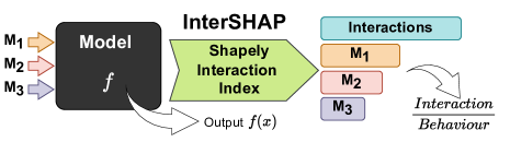
Figure 1: Overview of InterSHAP. The model (black box), takes three different modalities as input and produces an output $f(x)$. Through perturbations of the input modalities and observing the resulting changes in outputs, the Shapley interaction index (Grabisch and Roubens 1999) is used to dissect the model’s behaviour into modality contributions and cross-modal interactions. InterSHAP is defined as the ratio of interactions to model behaviour.

In medical decision-making, there is a growing trend toward utilising multimodal machine learning approaches that integrate multiple data sources to improve predictive and diagnostic tasks. These approaches acknowledge that medical data analysis is inherently multimodal, leveraging methods that are able to fuse heterogeneous data that includes clinical, genomic, and imaging modalities. Recent advancements in large multimodal models in the medical field, such as Google’s Med-PaLM (Tu et al. 2023) and Microsoft’s BiomedCLIP (Zhang et al. 2023), further highlight the utility of multimodal approaches in healthcare.

However, an inherent limitation of many of the current multimodal approaches pertains to their explainability. Thus, healthcare applications of machine learning are often left to rely on high-performance but opaque models that obscure the reasoning behind their predictions. Such models can accurately predict diagnoses, but these predictions may not reflect true causal relationships in the data (Han et al. 2022). The lack of explainability and transparency is widely recognized as a key barrier to the clinical adoption of ML models, as noted by policymakers such as the OECD (Anderson and Sutherland 2024) and emphasized in academic studies (Yang, Ye, and Xia 2022).

In response to the urgent need for XAI, numerous methods such as SHAP (Lundberg and Lee 2017) and LIME (Ribeiro, Singh, and Guestrin 2016) have emerged to explain the results of machine learning systems. While these have shown promise for unimodal models, there are few explanation methods that work effectively across data structures, meaning that cross-modal interactions can often not be quantified with unimodal methods. Multiple modalities allow a machine learning model to utilise and combine information from different sources, enabling cross-modal interactions that often lead to improved performance. However, simply identifying these interactions is insufficient for a meaningful interpretation of the model predictions. In this context, it is crucial to comprehend both the individual impact of each modality and their combined influence. Several methods, such as PID (Liang et al. 2023), EMAP (Hessel and Lee 2020), and SHAPE (Hu, Li, and Zhou 2022), have been developed to assess whether models learn cross-modal interactions. However, these methods are often (1) limited to only two modalities; (2) applied to the entire dataset, rather than individual samples; and (3) either require labelled data or are not performance-agnostic, which can lead to an incomplete understanding of cross-modal interactions.

In this paper, we introduce InterSHAP, a comprehensive, interpretable metric that quantifies the influence of cross-modal interactions on model behaviour. InterSHAP supports any number of modalities, provides local explanations, is agnostic to model performance, and works with unlabelled data. To our knowledge, our proposed variant of the Shapley interaction index is the first approach that is able to effectively separate cross-modal interactions from individual modality contributions. Figure 1 provides a schematic overview of InterSHAP. To validate the effectiveness of InterSHAP, we conduct extensive empirical analyses using synthetic datasets with either no synergy (no cross-modal interactions are needed to solve the task) or exclusively synergy (complete information can only be obtained as a result of cross-modal interaction across all modalities). The results demonstrate that InterSHAP can accurately detect a lack of cross-modal interactions ($0\%$) on datasets with no synergy, and $99.7\%$ on those with exclusive synergy, aligning precisely with the expected behaviour. Furthermore, we demonstrated that InterSHAP is extendable to more than two modalities and achieves favourable results at a local level with individual data points. Additionally, we test InterSHAP on two medical datasets to show its utility in a real-world setting. InterSHAP is not confined to medical domains and can be applied to models trained on any modality.

Our main contributions can be summarised as follows:

• Novel cross-modal interaction score InterSHAP. We introduce InterSHAP, the first model-agnostic cross-modal interaction score that operates with any number of modalities, offering both local and global explanations, applies to unlabelled datasets and does not rely on the model’s performance. We conducted extensive experiments on synthetic datasets and models to validate its functionality.

• Application to multimodal healthcare datasets. We demonstrate the benefits of InterSHAP on a cell type classification task based on multimodal protein and RNA data as well as a mortality prediction tasks.

• Open-source implementation with integration into the SHAP Package. We have developed an open-source implementation of InterSHAP that seamlessly integrates with the well-known SHAP visualisation package (Lundberg and Lee 2017). Code is available at github.com/LauraWenderoth/InterSHAP.

2 Related Work

Table 1: InterSHAP overcomes the limitations of other cross-modal interaction scores: it is unsupervised, performance agnostic, applicable to more than two modalities, and allows for dataset- (global) and sample-level (local) explainability.

Score Modalities $>2$ Local Unsupervised Performance Agnostic PID ✓ ✓ EMAP SHAPE ✓ InterSHAP ✓ ✓ ✓ ✓

Existing approaches like MM-SHAP (Parcalabescu and Frank 2023) and Perceptual Score (Gat, Schwartz, and Schwing 2021) focus on understanding the contributions of individual modalities rather than explicitly examining their interactions. They explain modality contributions in isolation without considering or quantifying cross-modal interactions within multimodal networks. In contrast, EMAP (Hessel and Lee 2020) and SHAPE (Hu, Li, and Zhou 2022) detect cross-modal interactions by analysing how perturbations to the input impact the model’s output. They systematically vary different modalities or combinations of modalities to assess their importance within the model. Another metric for detecting interactions, Partial Information Decomposition (PID) (Liang et al. 2023), quantifies synergy (interactions between modalities in a dataset with a combined effect surpassing individual contributions, indicating a non-additive relationship) in datasets, which can be interpreted as cross-modal interactions.

However, these existing approaches exhibit various limitations, summarised in Table 1. First, most of them restrict the analysis to just two modalities, which prevents them from being applied in domains that typically have more modalities, like in healthcare. Second, the results cannot be analysed at the level of individual samples, which is particularly critical for medical tasks where explainability for each patient is crucial. Third, some approaches necessitate the availability of labels, rendering them unsuitable for unlabelled datasets employed in self- or unsupervised learning scenarios. Fourth, certain methods assess interactions solely based on performance gain, rendering them highly performance-dependent. However, when assessing a model, it is crucial to understand how each interaction contributed to the present prediction without neglecting interactions only because the prediction was incorrect.

3 Methodology

We introduce InterSHAP to quantify cross-modal interaction learned by multimodal models while overcoming the limitations of SOTA explainability approaches. Following the definition of Liang, Zadeh, and Morency (2022), we define cross-modal interaction as a change in the model response that cannot be attributed to the information gained from a single modality alone, but arises only when both modalities are present. To ensure the accuracy of InterSHAP, we use the Shapley Interaction Index (SII), which has been shown to effectively capture model behaviour (Lundberg et al. 2020) and decompose unimodal feature interactions into its constituent parts (Ittner et al. 2021).

3.1 Preliminaries

Model Fusion.

To train multimodal models is model fusion, which comes in three types: (i) early fusion, which merges data features at model input, (ii) intermediate fusion, which combines data within the model, and (iii) late fusion, which combines the outputs of models trained on different individual data modalities (Stahlschmidt, Ulfenborg, and Synnergren 2022; Azam, Ryabchykov, and Bocklitz 2022).

Shapley Value.

The Shapley value $\phi$, from cooperative game theory, measures each feature’s contribution to overall performance via marginal contributions to feature coalitions (Roth 1988). In machine learning, a model $f_{M}$ is viewed as a coalition game with $M$ features or modalities as players. To avoid inefficient retraining, masking strategies are applied to features $j\notin S$, where $S\subseteq M$.

The Shapley value $\phi$ of a feature $i$ is calculated as the weighted average of their marginal contributions to all possible coalitions:

$$\phi_{i}(M,f) =\sum_{S\subseteq M\backslash\{i\}}\frac{|S|!(|M|-|S|-1)!}{|M|!}\Delta$$ (1)

$$\Delta =\left[f_{S\cup\{i\}}\left(S\cup\{i\}\right)-f_{S}\left(S\right)\right].$$

Shapley Interaction Index.

The Shapley Interaction Index (SII) (Grabisch and Roubens 1999), initially devised to quantify interaction effects between players in cooperative game theory, can be employed to discern interactions between features or modalities. We define its directly adapted version $\phi_{ij}(M,f)$ for $M$ modalities and a model $f$, where $i,j\in M$ (Lundberg et al. 2020) and $i\neq j$:

$$\phi_{ij}(M,f)=\!\!\sum_{S\subseteq M\backslash\{i,j\}}\!\!\frac{|S|!(M-|S|-2)!}{2(M-1)!}\nabla{ij}(S,f),$$ (2)

$$\nabla_{ij}(S,f)= \left[f_{S\cup\{ij\}}\left({S\cup\{ij\}}\right)-f_{S\cup\{i\}}\left({S\cup\{i\}}\right)\right.$$ (3)

$$\left.-f_{S\cup\{j\}}\left({S\cup\{j\}}\right)+f_{S}(S)\right].$$

The interaction index for a modality with itself, denoted as $\phi_{ii}$, is defined as the difference between the Shapley value $\phi_{i}$ and the sum of all interaction values:

$$\phi_{ii}(M,f)=\phi_{i}(M,f)-\sum_{j\in M}\phi_{ij}(M,f)\quad\forall i\neq j.$$ (4)

3.2 Global InterSHAP

We aim to quantify the impact of cross-modal interactions on model behaviour using InterSHAP. Model behaviour is a cumulative process, beginning with the model’s base output and progressively adding each modality and their interactions to shape the final prediction. To isolate interactions from the model behaviour, we apply the SII. Let $f\in\mathbb{R}^{c}$ be a trained model, where $c$ is the number of per-class probabilities, evaluated on a dataset with $N$ samples and $M$ modalities, represented as $\{(m_{1}^{i},\dots,m_{M}^{i})\}_{i=1}^{N}$ and corresponding labels $\{y^{i}\}_{i=1}^{N}$. The SII value $\phi_{ij}$ measures the interaction between modalities $i$ and $j$ for sample $a$. $\Phi_{ij}$ is defined as the absolute value of the mean over $\phi_{ij}$ of all samples in the dataset:

$$\Phi_{ij}=\left|\frac{1}{N}\sum_{a=1}^{N}\phi_{ij}(m_{1}^{a},\dots,m_{M}^{a},f)\right|,$$ (5)

resulting in the matrix $\Phi$ containing only positive values:

$$\Phi=\begin{bmatrix}\Phi_{11}&{\color[rgb]{0,0,0}\Phi_{12}}&\dots&{\color[rgb]{0,0,0}\Phi_{1M}}\\ {\color[rgb]{0,0,0}\Phi_{21}}&\Phi_{22}&\dots&{\color[rgb]{0,0,0}\Phi_{2M}}\\ \vdots&\vdots&\ddots&\vdots\\ {\color[rgb]{0,0,0}\Phi_{M1}}&{\color[rgb]{0,0,0}\Phi_{M2}}&\dots&\Phi_{MM}\end{bmatrix},$$ (6)

where interactions appear in green, while modality-specific contributions are shown in black. Note that, our choice of obtaining $\Phi_{ij}$ allows for a global interpretability view, accounting for opposing effects that may cancel out across dataset. This prevents score inflation and aligns with our main motivation – a general and robust measure of interaction strength. In turn, these are aggregated to obtain the total interactions contributions as well as the overall model behaviour:

$${Interactions}=\sum_{\begin{subarray}{c}i,j=1\\ i\neq j\end{subarray}}^{M}\Phi_{ij},\quad{Behavior}=\sum_{i,j=1}^{M}\Phi_{ij}.$$ (7)

Finally, these are used to calculate InterSHAP, which is the fraction of model behaviour that can be explained through cross-modal interactions:

$$InterSHAP=\frac{{Interactions}}{{Behavior}}.$$ (8)

3.3 Modality contributions

Based on the definition of cross-modal interactions in Equation 7, the contribution of all modalities $\mathcal{M}$ and the contribution of each modality $\mathcal{M}_{i}$ to the overall result is:

$$\mathcal{M}=1-{InterSHAP},\quad\mathcal{M}_{i}=\frac{\left|\Phi_{ii}\right|}{{Behaviour}}.$$ (9)

3.4 Local InterSHAP

After determining the amount of interactions that a model $f$ has learned across the entire dataset, we assess the extent to which cross-modal interactions among the $M$ modalities contribute to the model’s behaviour for each sample. Thus, we apply the definition of InterSHAP directly to a sample $a$:

$$I_{a}=\frac{\sum_{\begin{subarray}{c}i,j=1\\ i\neq j\end{subarray}}^{M}\varphi_{ij}^{a}}{\sum_{i,j=1}^{M}\varphi_{ij}^{a}},$$ (10)

where $\varphi_{ij}^{a}\!=\!\left|\phi_{ij}(\left(m_{1}^{a},\dots,m_{M}^{a}\right),f)\right|$, and $i,j\!\!\in\!\!\{1,\dots,M\}$. To determine if InterSHAP is effective at the level of all individual data points, we aggregate $I_{a}$ across the entire dataset to obtain the local interaction score for the dataset as a whole:

$$InterSHAP_{local}=\frac{1}{N}\sum_{a=1}^{N}I_{a}.$$ (11)

Table 2: Local and global InterSHAP values are presented in percentages for both the XOR function and the FCNN with early fusion on HD-XOR dataset with two modalities. EMAP_gap (EMAP - F1 of the model) and SHAPE indicate F1 score improvement from cross-modal interactions, with negative values signalling performance decline. For PID, the synergy value is provided, though it is not expressed in any standard unit. For all metrics, higher scores indicate greater measured cross-modal interactions. Results for the XOR function align with expectations, confirming the effectiveness of the InterSHAP implementation.

	Uniqueness		Synergy		Redundancy	Random
	XOR	FCNN	XOR	FCNN	FCNN	FCNN
InterSHAP	0.0	0.2 ±0.1	99.7	98.0 ±0.5	38.6 ±0.5	57.8 ±1.1
${\text{InterSHAP}_{local}}$	1.8	3.4 ±5.2	96.9	85.8 ±12.1	37.3 ±25.0	40.0 ±13.3
PID	0.01	0.01 ±0.01	0.39	0.39 ±0.01	0.14 ±0.02	0.48 ±0.01
EMAPgap	0	0 ±0	49.1	43.5 ±1.0	1.8 ±0.4	0.6 ±0.4
SHAPE	1.6	16.5 ±0.6	33.1	27.6 ±1.5	-47.1 ±0.5	15.1 ±1.9

3.5 Asymptotic Bound

InterSHAP is characterised by a computational complexity of $O(N^{M})$, where $N$ represents the number of samples and $M$ signifies the number of modalities (Grabisch and Roubens 1999; Lundberg et al. 2020). The constraint of exponential growth emerges with the increasing number of modalities rather than the feature count. InterSHAP’s dependency on the number of features within a modality follows a constant pattern, meaning its runtime remains unaffected by the feature count.

4 Experimental Validation on Synthetic Data

To verify InterSHAP’s functionality, we control three factors influencing cross-modal interactions: dataset synergy (non-additive interactions between modalities), model learning capacity, and metric effectiveness.

4.1 Setup

We utilise synthetic high-dimensional tabular datasets, generated using an XOR function (HD-XOR), with varying degrees of synergy to regulate the extent of cross-modal interactions. Each generated dataset contains 20,000 samples, with two to four modalities represented as 1D vectors consisting of around 100 features. The datasets are categorised on their degrees of synergy. Uniqueness represents datasets with no synergy, where all information is contained within a single modality. Synergy refers to datasets with complete synergy, where information is distributed across a number of modalities and can only be obtained through cross-modal interactions. Redundancy denotes datasets where the same information is present across modalities. Random applies to datasets with no meaningful information. For each number of modalities (two, three and four), we created a synergy, uniqueness and redundancy dataset as well as a random dataset for the case with two modalities.

To control for model variability in our experiments, we use the XOR function for the uniqueness and synergy datasets. The XOR function cannot be meaningfully applied to random and redundancy datasets, because it is unclear which information from each modality contributes to the solution, given the multiple possibilities. We train fully connected neural networks (FCNNs) on all datasets with three layers: input, hidden (half the input size), and output (half the hidden size). Three fusion strategies are tested: early fusion (data concatenated before input), intermediate fusion (data fused before the hidden layer), and late fusion (data fused before the output layer). Since early fusion captured the most cross-modal interactions, we use it in all subsequent FCNN experiments. Further details on the dataset generation and experimental setup are provided in Appendix A.

4.2 Results

Verification of InterSHAP. Generally, we anticipate that InterSHAP for the uniqueness dataset will show less cross-modal interaction (expected to be close to 0%) compared to the synergy dataset (expected to be close to 100%). For the random and redundancy datasets, it is unclear how many cross-modal interactions the FCNN should learn. In the redundancy setting, the FCNN might focus on just one modality or use all modalities since information is distributed across them. In the random setting, there is no inherent information, making the FCNN’s learning unpredictable.

Table 2 presents the results of the experiments conducted on the HD-XOR datasets. InterSHAP predicts the expected amount of cross-modal interaction in the XOR function with 0% cross-modal interaction for uniqueness and 99.7% for synergy. In contrast, the FCNN model showed an increase in cross-modal interaction for the uniqueness dataset (0.2% $\pm$ 0.1) and decrease in synergy (98.0% $\pm$ 0.5) for the synergy setting. This indicates that the FCNN does not fully capture the systematic structure underlying the dataset’s creation with the XOR function. Instead, it sometimes uses both modalities for predictions even when unnecessary, and conversely, may underutilise them when they are required.

InterSHAP indicates that the FCNN attributes approximately 40% of its behaviour to cross-modal interactions on the redundancy dataset. Especially noteworthy is the outcome on the random dataset, which shows that InterSHAP operates performance-agnostic, as only random performance could be achieved on this dataset. Nevertheless, the model appears to have learned something – though not relevant to the F1 Score – evidenced by approximately 60% of cross-modal interactions. In summary, InterSHAP demonstrates the expected behaviour and adequately quantifies cross-modal interaction within a model.

Modality Scalability.

To test InterSHAP’s scalability to more than two modalities, we create HD-XOR datasets with three and four modalities. The InterSHAP values for the FCNN with early fusion across uniqueness, synergy, and redundancy datasets are presented in Table 3.

Table 3: InterSHAP values, expressed as percentages, for FCNN with early fusion on HD-XOR datasets with two, three, and four modalities. The results indicate, that InterSHAP works for more than two modalities.

	Uniqueness	Synergy	Redundancy
2 Modalities	2.6 ±0.6	98.0 ±0.5	38.6 ±0.5
3 Modalities	0.6 ±0.2	88.8 ±0.5	51.9 ±0.3
4 Modalities	1.2 ±0.1	64.1 ±0.8	40.2 ±0.2

The expected behaviour is that InterSHAP values for three and four modalities should be the same or similar to those for two modalities, given that the dataset creation process remains unchanged except for the synergy setting. InterSHAP exhibits the expected behaviour on the uniqueness dataset, with values ranging from $0.6\pm 0.2$ to $2.6\pm 0.6$. Similarly, values on the redundancy setting show consistent behaviour with larger fluctuations, ranging from a minimum of $38.6\pm 0.5$ to a maximum of $51.9\pm 0.3$. However, for the synergy setting, InterSHAP indicates a decrease from $98\%$ cross-modal interactions to $64\%$ as the number of modalities increases.

Extension to Local Method.

InterSHAP can be applied to individual samples, as outlined in Section 3.4. InterSHAP values are averaged over each data point for three runs and standard deviation is calculated, as shown in Table 2.

On the HD-XOR uniqueness dataset using the XOR baseline function, the local method overestimates the synergy effect, with averages of 1.8%, compared to the global averages of 0%. Conversely, for the synergy setting, the local method underestimates the synergy effect, with averages of 96.9% locally compared to 99.7% globally. This difference is likely attributable to the masking error source. While this error averages out when considering the entire dataset, it is more pronounced at the data point level. The difference becomes more apparent when examining the FCNN results. Particularly noteworthy is the increased standard deviation, which indicates a discrepancy between data points. In contrast to the XOR function, this difference is caused by the neural network and reflects the model’s behaviour.

In summary, we have shown that with a controlled model (XOR), cross-modal interactions are slightly overestimated for datasets with near 0% synergy and slightly underestimated for datasets with near 100% synergy. For an overall interaction score across the entire dataset, we recommend using the global InterSHAP. However, if the goal is to understand the interaction score at the level of individual data points, local InterSHAP is more appropriate.

Comparison with SOTA.

To compare InterSHAP with SOTA cross-modal interaction scores, we calculated PID, EMAP and SHAPE, as shown in Table 2.

PID.  As expected, PID measures fewer cross-modal interactions on the uniqueness compared to the synergy dataset. However, PID is not able to quantify the extent of cross-modal interactions, unlike InterSHAP. In random and redundancy datasets PID also aligns with InterSHAP. Both show higher values for the random dataset than for the redundancy dataset, indicating that the model learned synergistic relationships.

EMAP.  For clearer comparison, we present EMAP_gap, calculated as EMAP minus the model’s F1 score (see Appendix C, Table 11), which reflects the extent of cross-modal interactions. Like other metrics, EMAP also follows the expected pattern, with less synergy observed for the uniqueness dataset than for the synergy dataset. However, EMAP measures no interaction in the model on the random dataset, because it is not performance-agnostic.

SHAPE.  SHAPE exhibits the expected behaviour on the baseline XOR function for uniqueness and synergy datasets but not for the FCNN model. There are major deviations between the baseline XOR and FCNN results that are not due to model behaviour. While the uniqueness dataset shows similar values for the baseline XOR, the FCNN results differ significantly, with $16.5\pm 0.06$ for uniqueness. Additionally, the redundancy dataset results do not align with the previous three metrics. We attribute these discrepancies to the masking and calculation of base values.

4.3 Visualisation

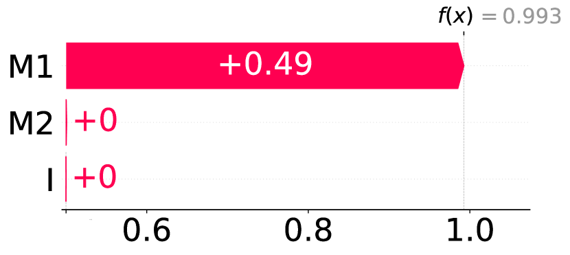
(a) Uniqueness 1

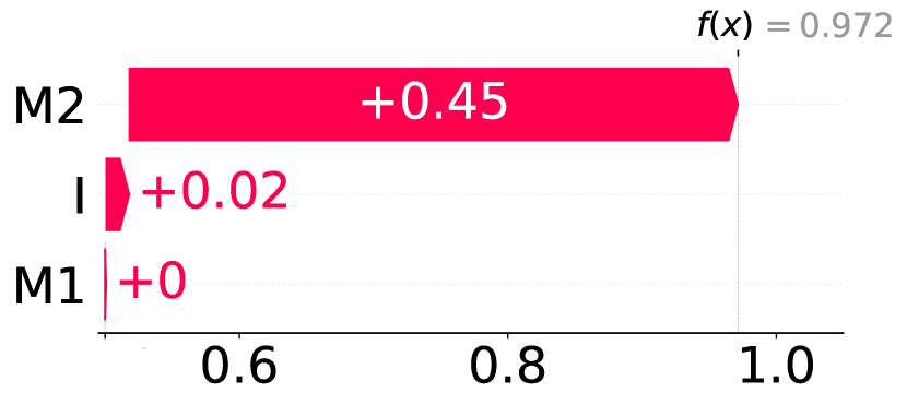
(b) Uniqueness 2

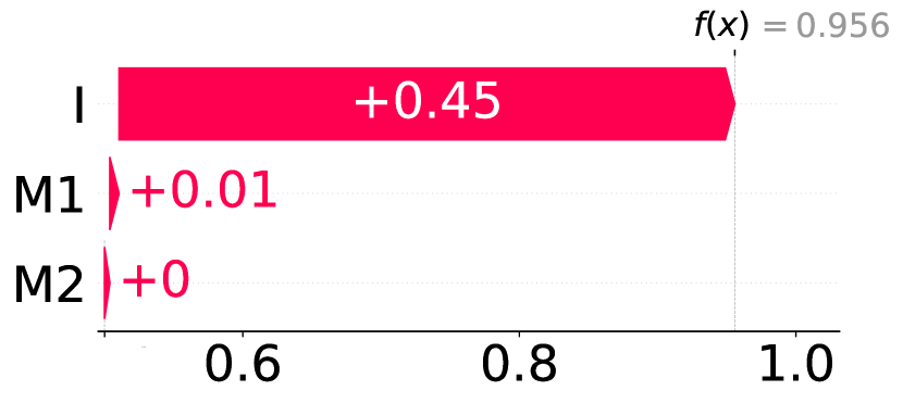
(c) Synergy

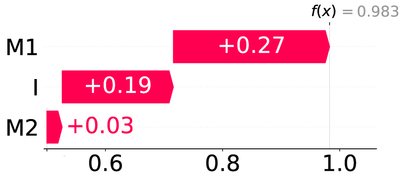
(d) Redundancy

(e) Random

Figure 2: Visualisation of InterSHAP using the SHAP package integration (Lundberg and Lee 2017). The results on the HD-XOR datasets with two modalities for FCNN with early fusion are presented. The x-axes show predicted class probabilities, with a baseline of approximately 0.5 due to the binary classification. M1 represents modality 1, M2 modality 2, and I interactions.

We designed InterSHAP to be compatible with the visualisation modules of the SHAP implementation (Lundberg and Lee 2017). Figure 2 illustrates the breakdown of model behaviour on the HD-XOR datasets into their components. This representation uniquely shows the relevance of modalities in absolute numbers in addition to cross-modal interactions. For instance, in Figure 2 (d), it is evident that modality 1 is, on average, more important for the prediction than the interactions. Additionally, the prediction on the random dataset is significantly less certain, with an average probability of only 79.8%, compared to 95-99% for the other datasets.

5 Application to Healthcare Domain

The importance of cross-modal interactions in real-world healthcare datasets is examined by analysing two publicly available multimodal datasets with two modalities with distinct input types.

The first dataset, multimodal single-cell (Burkhardt et al. 2022), includes RNA and protein data from 7,132 single cells of CD34+ haematopoietic stem and progenitor cells from three donors. Its classification task spans four cell types: neutrophil progenitor (3,121), erythrocyte progenitor (3,551), B-lymphocyte progenitor (97), and monocyte progenitor (363). The data was reduced to 140 proteins and 4,000 genes and split into training (4,993), validation (1,069), and test (1,070) sets (70:15:15 ratio).

The second dataset, MIMIC-III (Johnson et al. 2016), contains anonymised clinical data from ICU patients at Beth Israel Deaconess Medical Center (2001–2012). It includes time series data (12 physiological measurements taken hourly over 24 hours, vector size $12\times 24$) and static data (5 variables like age, vector size 5). The dataset has 36,212 data points, and is split into training (28,970), validation (3,621), and test (3,621) sets (80:10:10 ratio) (Liang et al. 2021). The tasks are binary ICD-9 code prediction (group 1) and 6-class mortality prediction. Preprocessing follows Liang et al. (2021).

We use FCNN with all three fusion methods described in Section 4.1 on the multimodal single-cell dataset. For the MIMIC-III dataset, we train two models from MultiBench (Liang et al. 2021): the MultiBench baseline, which combines an MLP for patient information and a GRU encoder, and the MVAE, which uses a product-of-experts mechanism to combine latent representations from an MLP and a recurrent neural network. Table 4 presents the results concerning the amount of cross-modal interactions for each dataset.

Table 4: Cross-modal interactions scores on the multimodal single-cell dataset for FCNN with early, intermediate and late fusion. InterSHAP aligns with other SOTA methods, capturing the decline in cross-modal information from early to late fusion.

	Single-Cell
	early	intermediate	late
InterSHAP	1.9 ±0.4	1.5 ±0.4	0.4 ±0.1
PID	0.08 ±0.01	0.08 ±0.01	0.06 ±0.0
EMAPgab	0 ±0	0 ±0	0 ±0
SHAPE	1.0 ±0.2	0.7 ±0.2	0 ±0

5.1 Multimodal Single-Cell

For the multimodal single-cell dataset, we trained three FCNNs using early, intermediate, and late fusion (performance details in Appendix C), and calculated InterSHAP, PID, and EMAP for each model. As shown in Table 4, InterSHAP values range from 0.4% to 1.9%, indicating minimal learned cross-modal interactions. A consistent pattern is observed whereby cross-modal interactions decrease from early to late fusion, which is in accordance with findings from synthetic datasets (see Appendix C.1).

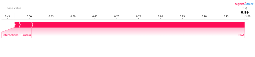
(a) Explanation over the whole dataset

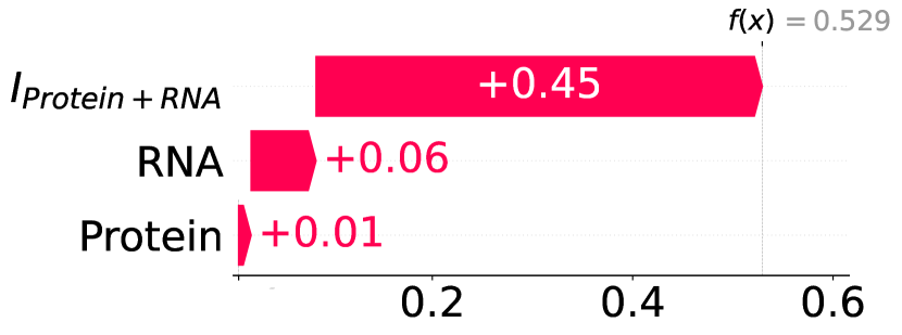
(b) B-Cell Progenitor

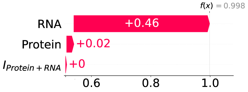
(c) Erythrocyte Progenitor

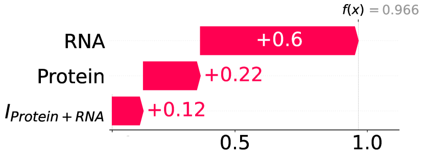
(d) Monocyte Progenitor

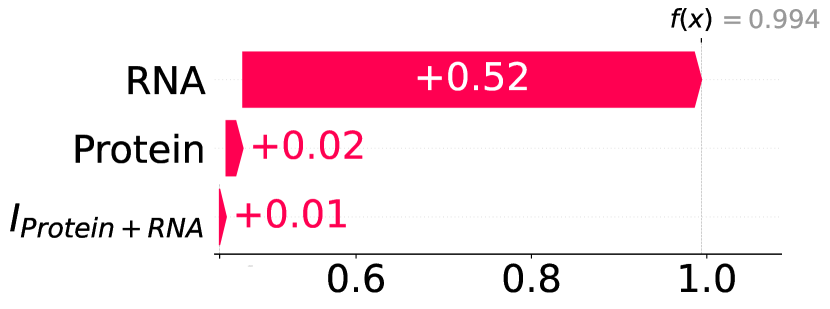
(e) Neutrophil Progenitor

Figure 3: SHAP visualisations of InterSHAP computed interactions and modality contributions derived from the FCNN early fusion model trained on the multimodal single-cell dataset. (a) Force plot of model’s behaviour on the whole dataset, with the x-axis representing the class probability of the highest probability class. (b)-(d) Breakdown by predicted class.

We employ SHAP visualisations, as shown in Figure 3, to illustrate modality contributions by predicted class. A clear distinction in measured cross-modal interactions is observed between the larger classes (erythrocytes and neutrophils, comprising 93.5% of the training dataset) and the smaller classes (monocytes and B-cells). For smaller classes, the model’s predictions depend largely on cross-modal interactions, while for larger classes, RNA is the most significant factor influencing the prediction.

The absence of ground truth in real-world datasets is a significant limitation, as the level of synergy or redundancy is unknown. To address this, additional cross-modal interaction scores, PID and EMAP, were computed for comparison with InterSHAP in Table 4. PID displayed behaviour similar to InterSHAP across the three fusion methods, with higher values for early fusion and lower for late fusion. However, PID indicated much higher synergy within the dataset, which is expected since PID focuses on the dataset rather than directly accounting for model behaviour. The authors also note that PID measures consistently exceed those of the dataset (Liang et al. 2023, 30). Therefore, to quantify the extent of cross-modal interactions utilised by a model in its predictions, InterSHAP is a more effective solution. In contrast, EMAP did not detect cross-modal interactions in any models. This difference likely arises because EMAP targets performance rather than directly measuring model behaviour. As depicted in Figure 3, smaller classes benefit significantly from interactions. However, due to their underrepresentation in the dataset, their overall impact on performance remains limited.

We can conclude that models trained on the multimodal single-cell dataset utilise minimal cross-modal interactions to solve the classification task. Exceptions to this are the smaller classes, for which integrating both modalities and concluding information from cross-modal interactions appears more relevant.

5.2 MIMIC III

For the MIMIC dataset, we trained a baseline model and the MVAE model provided in the MultiBench (Liang et al. 2021) (details in Appendix B).

From the cross-modal interactions presented in Table 5, we observe a consistent pattern: the baseline model shows fewer cross-modal interactions than the more sophisticated MVAE model. InterSHAP values vary between tasks. For deciding if the diagnosis is in ICD-9, lower interactions are measured, ranging between 1.2% and 6.8%, compared to the more challenging task of determining mortality, which shows higher interactions around 12%.

Comparing InterSHAP with PID and EMAP reveals similar behaviour to the multimodal single-cell dataset, discussed above. PID mirrors the behaviour of InterSHAP but with higher synergy values, while EMAP does not indicate performance-relevant cross-modal scores for the ICD-9 task, but does for the mortality task. This behaviour is expected and aligns well with InterSHAP, which, as it measures performance independently, captures even small amounts of cross-modal interaction, whereas EMAP captures larger performance-relevant ones.

Table 5: Cross-modal interactions scores on the MIMIC III dataset for baseline model and MVAE model from MultiBench implementation. InterSHAP aligns with other SOTA methods, capturing greater cross-modal interaction in the baseline compared to MVAE, while uniquely quantifying the proportional contribution of cross-modal interactions.

ICD-9 Mortality baseline MVAE baseline MVAE InterSHAP 1.2 _±0.2 6.8 _±1.3 11.0 _±0.5 12.3 _±2.8 PID 0.06_±0.01 0.09 _±0.01 0.10 _±0.01 0.11 _±0.01 EMAP_gap 0 _±0 1.2 _±0.0 $-$0.8 _±0.1 0.9 _±0.1 SHAPE 0.2 _±0 0.6 _±0 0.2 _±0.2 0.7 _±0.2

6 Discussion and Future Work

InterSHAP quantifies interaction strength as an interpretable percentage and works effectively with unlabelled data. Although the value of a performance-agnostic metric may be debated, InterSHAP is particularly useful for model development and debugging. For example, in our imbalanced single-cell study, smaller classes with minimal impact on the overall performance exhibited a higher reliance on cross-modal interactions, highlighting areas where modality integration could be improved. By capturing all cross-modal interactions – not just those linked to performance – InterSHAP provides deeper insights into low-performing models and can conclusively identify the absence of interactions, avoiding spurious results seen with performance-dependent methods.

Despite these benefits, we note some limitations of InterSHAP. The first is the exponential increase in runtime with the number of modalities, as all possible coalitions must be computed due to the lack of general approximation methods for SII. However, this is less critical in practice, as models are typically trained on fewer than ten modalities (Barua, Ahmed, and Begum 2023; Xu et al. 2024). Future work could explore approximation methods to address this computational challenge.

The second limitation is that we could not clearly demonstrate that InterSHAP functions as intended for synergy datasets with more than two modalities due to two factors: (1) The synergy in the training dataset decreases as the number of modalities increases. This phenomenon is attributed to the definition of XOR for more than two modalities: only one occurrence of 1 will result in the label being true, with the rest being 0. Consequently, if a 1 is present in two modalities, the label (i.e., false) is already known. (2) The F1 score decreases: 94.4 $\pm$ 0.3 for two modalities, 79.2 $\pm$ 0.2 for three modalities, and 76.4 $\pm$ 0.2 for four modalities. This indicates that the synergy present in the dataset is not fully learned, leading to the model likely relying less on cross-modal interactions for prediction. The observed decrease is likely attributable to the two factors, although the potential contribution of InterSHAP cannot be ruled out. Although InterSHAP relies on the Shapley Interaction Index (SII) and captures pairwise modality interactions, it may not fully address complex cross-modality interactions. Future research could explore alternative interaction measures than the SII. Other unimodal indices at the feature level could be also applied to quantify cross-modal interactions in datasets with more than two modalities to overcome this limitation. Potential alternatives for evaluation include Faith-SHAP (Tsai, Yeh, and Ravikumar 2023) and the Shapley-Taylor Interaction Index (Sundararajan, Dhamdhere, and Agarwal 2020).

7 Conclusion

We introduce InterSHAP, a multimodal explainability metric designed to quantify cross-modal interactions and modality contributions. InterSHAP provides a straightforward interpretation of cross-modal interactions, expressed as a percentage of overall model behaviour, which can be applied to multimodal learning tasks with any number of modalities. Besides explainability, it allows for investigating the capabilities of different model architectures in how they exploit multimodal interactions across real-world datasets. As such, InterSHAP overcomes the limitations of existing methods, akin to constraints to only two modalities and the lack of reliable, performance-independent methods. Our experiments on synthetic and real-world data demonstrate the ability of InterSHAP to accurately measure the presence (or absence) of cross-modal interactions, while allowing for global (dataset-level) and local (sample-level) explanations.

Appendix A Synthetic Data Generation

Since synthetic dataset generation presents inherent challenges, including data distribution bias, insufficient noise levels, over-smoothing, and inconsistencies (Hao et al. 2024), we draw inspiration from two existing approaches to create the synthetic datasets (Liang et al. 2023; Hessel and Lee 2020) to formulate our synthetic data generation strategy HD-XOR. Additionally, we use a second synthetic data generation method called SUM. For each generation method, there exists an ensemble of datasets displayed in Table 6. An ensemble refers to a set of datasets created using the same method (HD-XOR or SUM) with varying degrees of synergy, from setting uniqueness (no synergy) to setting synergy (full synergy). In the following, we will first present our strategy (HD-XOR) for creating the dataset ensemble. Subsequently, we will briefly introduce the strategy (SUM dataset) described by Liang et al. (2023).

High-Dimensional XOR Dataset.

Algorithm 1 Generate synthetic data

1:procedure data_distribution(setting, $N$: number of samples, $M$: number of modalities, dims $\in\mathbb{Z}^{M},$)

2:  $\iota\leftarrow 2$

3:  if $M\geq 3\quad\land\quad$setting is synergy then

4:   $\iota\leftarrow M$

5:  end if

6:  $I,y\leftarrow\{i_{1}^{i},\dots,i_{M}^{i}\}_{i=1}^{N},\{y^{i}\}_{i=1}^{N}\quad\{i_{1}^{i},\dots,i_{M}^{i}\},y^{i}=\text{GEN\_INFO}(A=\iota)$

7:  

8:  if setting is redundancy then

9:   $M_{m}\in\mathbb{R}^{\text{dims}_{m}\times 2\cdot d}\sim\mathcal{U}(-0.5,0.5),\quad\forall i\in\{1,\dots,M\}$

10:   $x^{i}\leftarrow[i_{1}^{i},i_{2}^{i}]$,  $\forall i\in\{1,\dots,N\}$

11:   $X\leftarrow\{x_{1}^{i},\dots,x_{M}^{i}\}_{i=1}^{N}$

12:  else if setting is uniqueness then

13:   unique modality $u\in\{1,\dots,M\}$

14:   $M_{m}\in\mathbb{R}^{\text{dims}_{m}\times 2\cdot d}\sim\mathcal{U}(-0.5,0.5),\quad\forall i\in\{1,\dots,M\}$

15:   $x^{i}\leftarrow[i_{1}^{i},i_{2}^{i}]$,  $\forall i\in\{1,\dots,N\}$

16:   $x_{j}\in\mathbb{R}^{2\cdot d}\sim\mathcal{N}(0,1),\quad\forall j\{1,\dots,M\},j\neq u$

17:   $X\leftarrow\{x_{1}^{i},\dots,x_{u}^{i},\dots,x_{M}^{i}\}_{i=1}^{N}$

18:  else if setting is synergy then

19:   $M_{m}\in\mathbb{R}^{\text{dims}_{m}\times d}\sim\mathcal{U}(-0.5,0.5),\quad\forall i\in\{1,\dots,M\}$

20:   $X\leftarrow I$

21:  end if

22:  $X\leftarrow\{M_{1}\cdot x_{1}^{i},\dots,M_{M}\cdot x_{M}^{i}\}_{i=1}^{N}$

23:  return $X,y$

24:end procedure

1:procedure gen_info($A$: number of information dimensions)

2:  $i\leftarrow\left\{i_{a}\in\{0,1\}\sim\text{Bernoulli}(\frac{1}{2})\right\}_{a=1}^{A}$

3:  $y\leftarrow i_{1}\oplus i_{2}\oplus\dots\oplus i_{A}=\bigoplus_{a=1}^{A}i_{a}$

4:  Project $i$ in higher dimensional space:

5:  for $a\leftarrow 1$ to $A$ do

6:   if $i_{a}$ is 0 then

7:     $i_{a}\leftarrow i_{a}\in\mathbb{R}^{d}\sim\mathcal{N}(-0.35,1),\quad a\in\{1,\dots,A\}$

8:   else

9:     $i_{a}\leftarrow i_{a}\in\mathbb{R}^{d}\sim\mathcal{N}(0.35,1),\quad a\in\{1,\dots,A\}$

10:   end if

11:  end for

12:  return $i,y$

13:end procedure

The first synthetic dataset generation strategy is the high-dimensional XOR (HD-XOR). This method builds on the XOR function and generates high-dimensional datasets with any number of modalities and dimensions. To construct the HD-XOR dataset, we drew inspiration from methodologies proposed by Hessel and Lee (2020) and Liang et al. (2023).

The procedure to generate datasets using HD-XOR is described in Algorithm 1 in detail. Firstly, for each sample in the dataset, two numbers, denoted by $i_{1}$ and $i_{2}$, are randomly drawn from a fair Bernoulli distribution representing binary features. Suppose the synergy setting involves more than two modalities, as many numbers as modalities are drawn (line $2-5$). The label for each data point is then calculated using the XOR operation. Subsequently, $i_{1}$, $i_{2},\dots i_{M}$, are projected into a higher dimensional space using a normal distribution as described in (Hessel and Lee 2020). To obtain vectors with the information encoded by the binary integers, vectors from normal distributions with different mean values (negative for $0$, positive for $1$).

Table 6: Overview of generated synthetic datasets using two different generation methods, HD-XOR and SUM. The arrows indicate the degree of synergy in the dataset. A red arrow ($\downarrow$) signifies no synergy, a green arrow ($\uparrow$) indicates maximum synergy, and a yellow arrow ($\leftrightarrow$) represents moderate synergy. The question marks (?) denote uncertainty about the amount of synergy in the dataset, as it was created with maximum redundancy.

2 Modalities		3 Modalities	4 Modalities
HD-XOR	SUM	HD-XOR	HD-XOR
Uniqueness $\downarrow$ Synergy $\uparrow$ Redundancy ? Random ?	Uniqueness 1 $\downarrow$ Uniqueness 2 $\downarrow$ Mix 1 $\leftrightarrow$ Mix 2 $\leftrightarrow$ Synergy $\uparrow$ Redundancy ?	Uniqueness $\downarrow$ Synergy $\uparrow$ Redundancy ?	Uniqueness $\downarrow$ Synergy $\uparrow$ Redundancy ?

Subsequently, the information of the vectors must be distributed for the three distinct settings (redundancy, synergy, and uniqueness), employing a methodology analogous to that described in (Liang et al. 2023). In the redundancy setting, the variables $i_{1}$ and $i_{2}$ are concatenated and then copied $M$ times (where $M$ represents the desired number of modalities) for each sample. In the uniqueness setting, the components $i_{1}$ and $i_{2}$ are also concatenated but only written to the desired modality. All other modalities are filled with vectors drawn from a normal distribution with a mean value of 0. Finally, in the synergy setting, the components $i_{1}$, $i_{2},\dots i_{M}$ are distributed according to the modalities $1,2,\dots M$, respectively. To generate the desired dimensions, we draw $M$ matrices (one for each modality) from a uniform distribution. The matrix of each modality is multiplied element-wise with the corresponding normalised vector of unit length belonging to the same modality. This ensures that each vector in each modality is unique in the redundancy setting. The labels remain unchanged during the generation of the modalities. Additionally, we created a random dataset to evaluate behaviour on data where nothing meaningful can be learned. The vectors for the modalities are randomly generated with the desired dimensions and a mean of 0, while the labels are randomly selected from 0 and 1.

The HD-XOR dataset faces limitations when applied to more than two modalities in the synergy setting. For more than two modalities, the dataset no longer contains maximum synergy because XOR is defined as the sum of all integers to be one: $\sum_{a=1}^{M}i_{a}=1$. When there are already two positive values in the first modalities, the label is known to be negative. Thus, we know that synergy decreases with an increasing number of modalities.

SUM Dataset.

Additionally, we employ a second strategy to generate synthetic datasets for two modalities from Liang et al. (2023) to validate the functionality of InterSHAP across a diverse range of datasets. Like the HD-XOR dataset, the SUM dataset consists of an ensemble of datasets with varying levels of synergy. In addition to the three previously described settings — synergy, redundancy, and uniqueness — this generation approach allows for creating mixed datasets containing a mixture of unique and synergistic information.

To create the SUM datasets, we draw three vectors, $x_{1}$, $x_{2}$, and $r$, from a normal distribution and normalise them. We then concatenate the vectors $x_{1}$ and $r$ as well as $x_{2}$ and $r$ to form a vector for each modality, containing modality-specific information (denoted by $x$) and shared information (denoted by $r$). We use different parts of the vector to calculate the labels depending on the desired setting (uniqueness, synergy, redundancy, mix). Regarding redundancy, we consider only the component $r$ to ensure information redundancy across both modalities. For uniqueness, we use either the subcomponent $x_{1}$ or $x_{2}$. For synergy, both subcomponents $x_{1}$ and $x_{2}$ contribute to the calculation of the label. For the mix setting, we combine parts of $x_{1}$ and $x_{2}$. We use a sum function to calculate the labels, hence the name. For binary labels, the label is assigned 1 if the sum is greater than 0.5, otherwise 0.

The SUM dataset is limited in the synergy setting because the sum of one modality alone can exceed or be very close to 0.5, making the second vector unnecessary or resulting in guesses that deviate from the expected 50% probability in binary classification.

Appendix B Experimental Setup

B.1 Synthetic Datasets

We created synthetic datasets with varaying degrees of synergy using two distinct methods HD-XOR and SUM described in Section Synthetic Data Generation. For each generation method, there exists an ensemble of datasets displayed in Table 6. An ensemble refers to a set of datasets created using the same method (HD-XOR or SUM) with varying degrees of synergy, from setting uniqueness (no synergy) to setting synergy (full synergy).

The generated datasets consist of 20,000 samples each, with specific dimensionality configurations customised for individual modalities. The two-modal configuration of the HD-XOR datasets comprise dimensions of 110 and 90, while the SUM datasets feature dimensions of 100 for both modalities. For the HD-XOR datasets incorporating three, four, and five modalities, the dimensions are adjusted accordingly: (110, 90, 100), (110, 90, 100, 110), and (110, 90, 100, 110, 90). Each dataset is partitioned into three subsets - validation, testing, and training - with 15% of the samples allocated to the validation and testsets and the remaining 70% designated for training purposes. Moreover, the number of output classes remains fixed at two for both datasets.

B.2 Healthcare Datasets

We use two publicly available multimodal datasets. The first is called multimodal single-cell dataset and includes surface proteins and RNA sequencing modalities from hematopoietic stem cells. The second dataset is the MIMIC III dataset, which contains clinical data from intensive care units. This dataset comprises general patient data and time-series data from sensors used in intensive care.

Mulitmodal Single-Cell.

The Multimodal Single-Cell dataset, constructed by Burkhardt et al. (2022), integrates multi-omics data comprising gene expression profiles (RNA) and protein levels (protein) of single cells derived from mobilised peripheral CD34+ haematopoietic stem and progenitor cells isolated from three healthy human donors. Each cell within the dataset is assigned a cell type, including mast cell progenitor, megakaryocyte progenitor, neutrophil progenitor, monocyte progenitor, erythrocyte progenitor, haematopoietic stem cell, and B-cell progenitor.

Table 7: Details of Single Cell.

Class Distribution
Neutrophil	Erythrocyte	B-Lymphocytes	Monocyte
43.7%	49.8%	1.4%	5.1%

Preprocessing.  To facilitate analysis, a subset of four cell classes was selected, comprising two physiologically frequent cell classes, neutrophil progenitor and erythrocyte progenitor, which are overrepresented in the dataset, and two rarer cell classes, B-lymphocytes progenitor and monocyte progenitor. This resulted in 7132 data points, with a class distribution of 3121, 3551, 97, and 363, respectively. Furthermore, the surface protein modality was randomly reduced to 140 proteins, and the RNA modality was reduced to 4000 genes. Furthermore, the dataset is organised into training, validation, and test sets following a 70:15:15 split, respectively, yielding 4,993 training data points, 1,069 validation data points, and 1,070 test data points.

MIMIC III.

The Medical Information Mart for Intensive Care III (MIMIC III) dataset is a comprehensive collection of deidentified clinical data from patients treated in intensive care units at Beth Israel Deaconess Medical Center in Boston, Massachusetts, USA between 2001 and 2012 (Johnson et al. 2016).

Table 8: Details of MIMIC III, ICD 1 and mortality.

Class Distribution ICD Mortality No Yes 1d 2d 3d 7d 1 year $>$ 1 year 82.5% 17.5% 76.0% 0.4% 1.3% 1.0% 11.0% 10.3%

Preprocessing.  The dataset was preprocessed by Liang et al. (2021), who followed the preprocessing protocol of Purushotham et al. (2018) and reported that the process took approximately one to two weeks. The original dataset contained mistakes due to noise, missing values, outliers, duplicate or incorrect records, and clerical errors, as detailed in (Purushotham et al. 2018).

The preprocessed dataset comprises two modalities: time series data and static information on patients. The time series data comprises 12 time-stamped, nurse-verified physiological measurements, including heart rate, arterial blood pressure, fluid balance, and respiratory rate, taken every hour over a 24-hour period, resulting in a vector of size $12\times 24$. In contrast, the static data comprises five medical information variables, including the e.g patient’s age, represented in a vector of size five.

The available tasks comprise two ICD-9 code predictions and a mortality prediction. The ICD-9 code predictions entail a binary classification to determine whether a patient fits any ICD-9 code within group 1 (140-239) or group 7 (460-519). The International Classification of Diseases (ICD) is a widely recognised classification system for medical diagnoses published by the World Health Organisation (WHO). It provides a standardised framework for coding and categorising diseases, allowing for accurate and consistent reporting of health information (World Health Organization and others 1978). We only used ICD-9 group 1 for our experiments. The mortality prediction, on the other hand, is a six-class prediction to determine whether the patient dies within one day, two days, three days, one week, one year, or longer than one year.

Following the split proposed by Liang et al. (2021), the data was randomly divided into three sets: a training set, a validation set, and a test set with a ratio of 80:10:10, respectively. This resulted in 28,970 training data points, 3,621 validation data points, and 3,621 test data points, for a total of 36,212 data points. Please refer to Table 8 for further details.

Access Restrictions and Privacy.  The data has been deidentified in accordance with the relevant access restrictions and privacy considerations. This process involved removing identifying data elements such as telephone numbers and addresses. For further details, please refer to Johnson et al. (2016). Furthermore, all researchers working with this dataset must have completed courses in the protection of human research participants, including those pertaining to HIPAA (Health Insurance Portability and Accountability Act) requirements.

B.3 Models

The model is one of the three key components influencing the outcome of cross-modal interaction. Therefore, we use two models: a baseline based on the XOR function and a neural network. This approach allows us to control the model behaviour with the baseline, ensuring that the only uncontrolled component is the cross-modal interaction metric.

XOR Function.

The baseline refers to the function underlying the creation of the HD-XOR dataset. We utilise the XOR function for the controlled setting because it consistently produces the correct output, ensuring that the model reflects the maximum synergy in the dataset. The baseline model $f$ is described in Algorithm 2. Here, $i=[i_{1},i_{2},\ldots,i_{M}]$ represents the different modalities, while $[1.0,0.0]$ and $[0.0,1.0]$ denote the class-wise probabilities. The function get_unique(setting) in line 3 determines which modality contains the information and returns the corresponding integer.

Algorithm 2 Baseline XOR Function $f$

1:procedure XOR($i=[i_{1},i_{2},\ldots,i_{M}]$, setting)

2:  if setting $==$ uniqueness then

3:   unique_modality $\leftarrow$ get_unique(setting)

4:   $i\leftarrow i[\text{unique\_modality}]$

5:  end if

6:  if $\sum_{a=1}^{M}i[a]==1$ then

7:   return $[1.0,0.0]$

8:  else

9:   return $[0.0,1.0]$

10:  end if

11:end procedure

Table 9: InterSHAP values are depicted as percentages for the FCNN with early fusion on SUM datasets. InterSHAP measures the fewest cross-modal interactions in uniqueness datasets and the most in synergy datasets. Mixed datasets, as expected, fall between synergy and uniqueness, indicating that InterSHAP accurately quantifies gradations of cross-modal interactions.

	Uniqueness 1	Uniqueness 2	Mix 1	Mix 2	Synergy	Redundancy
InterSHAP	2.6 $\pm$ 0.6	2.3 $\pm$ 0.3	9.7 $\pm$ 0.9	7.1 $\pm$ 0.5	15.1 $\pm$ 0.5	10.5 $\pm$ 0.2
${\text{InterSHAP}_{local}}$	9.3 $\pm$ 10.2	9.0 $\pm$ 12.7	14.7 $\pm$ 9.9	13.8 $\pm$ 9.8	22.1 $\pm$ 11.2	22.3 $\pm$ 13.3

It is important to note that the fundamental XOR function only applies to synergy and all uniqueness datasets. This limitation arises due to the necessity of determining which information from the modalities is included in the calculation. For the redundancy setting, however, it is unclear whether a modality can be entirely disregarded or only a portion. Moreover, the XOR function does not apply to random datasets, as it was not the basis for their creation.

FCNN.

For the synthetic datasets, fully connected neural networks (FCNNs) comprising three layers are employed. In an FCNN, each neuron in one layer is connected to every neuron in the adjacent layer. The hidden dimensions are half the input dimensions, and the output dimensions are half the hidden dimensions. Three different fusion strategies are examined: early, intermediate, and late fusion. Early fusion involves concatenating or fusing the data before inputting it into the network. Intermediate fusion occurs before the hidden layer, while late fusion occurs before the output layer.

We experimentally validate InterSHAP starting with two modalities, followed by scalability to more than two modalities, and then extending to the local method, with subsequent visualisation options available due to integration with the SHAP package (Lundberg and Lee 2017). Finally, we will compare InterSHAP with existing cross-modal interaction scores on synthetic datasets.

MultiBench Baseline.

We use the baseline provided by the MultiBench implementation (Liang et al. 2021). The baseline combines a multi-layer perception (MLP) for patient information and a gated recurrent unit (GRU) encoder to process sequential data physiological measurements. Their outputs are concatenated in a fusion layer, forming a joint representation for classification through an MLP classification head with two hidden layers.

MVAE.

The MMultimodalVariational Autoencoder (MVAE) (Wu and Goodman 2018) is structured similarly to the baseline but employs a different fusion mechanism. For our implementation, we utilise the MultiBench implementation (Liang et al. 2021) without any alterations. The encoder consists of an MLP for patient information and a time series encoder for physiological measurements (recurrent neural network), which maps to a 200-dimensional vector in the latent space. The fusion involves using a product-of-experts mechanism to combine these latent representations, which are subsequently utilised for classification using an MLP.

B.4 Implementation

We develop an open-source implementation of InterSHAP, availble at github.com/LauraWenderoth/InterSHAP. This implementation includes InterSHAP alongside other methods such as PID, EMAP, and SHAPE. Additionally, our implementation seamlessly integrates with the widely-used SHAP visualisation package (Lundberg and Lee 2017). We employed a masking strategy by replacing the modalities of one data point with those from another data point drawn from the training data. This process was repeated $n$ times, and the results were averaged. For the target, we chose the probabilities of classification, specifically the highest class probability, because it ensures performance independence and represents the decisive outcome.

For PID, we use the CVX estimator and report the synergy value as the cross-modal interaction score. The macro F1 score is chosen as the target metric for both EMAP and SHAPE, and they are computed without further modifications. EMAP was calculated using an open-source implementation, whereas SHAPE required re-implementation based on the original paper, assuming the model always predicts the majority class to establish its baseline performance.

Training Details.  All training runs with synthetic data were conducted using three seeds: 1, 42, and 113. The learning rate was set at $1e-4$ without early stopping, and the optimiser used was Adam with a weight decay of $1e-4$. Models with two and three modalities were trained for 200 epochs, while models with four were trained for 250 epochs.

Appendix C Additional Results

C.1 Synthetic Data

Consistency of InterSHAP.

We tested InterSHAP on another data generation strategy to ensure its consistent, correct performance. Table 9 displays the outcomes of InterSHAP conducted on FCNNs with early fusion trained on each SUM dataset. The results demonstrate that InterSHAP effectively quantifies cross-modal interactions as intended, with minimal cross-modal interactions detected for uniqueness settings ($2.6\pm 0.6$ for uniqueness 1 and $2.3\pm 0.3$ for uniqueness 2), maximal for the synergy setting ($10.5\pm 0.2$), and falling in between for mixed synergy settings ($9.7\pm 0.5$ for mix 1 and $7.1\pm 0.5$ for mix 2). This aligns with the anticipated behaviour.

Compared to the XOR dataset, the cross-modal interactions computed by InterSHAP are generally smaller. Even in the synergy setting, only 15% of the model behaviour is attributed to cross-modal interactions. This behaviour is supported by the F1 scores, which indicate that 79% can be achieved with a single modality on average while using both modalities yields 87.6% on average. Therefore, it can be inferred that the dataset inherently contains less synergy than the XOR dataset.

Examining the results for InterSHAP${}_{l}ocal$, on average, higher synergy is estimated, albeit with a higher standard deviation. However, it is also evident here that InterSHAP${}_{l}ocal$ estimates less synergy for both unique settings than the mixed settings and, on average, the most for the synergy setting. In conclusion, InterSHAP is a reliable metric for cross-modal interaction for two modalities.

Effect of Fusion Method on Interactions.

To determine the most effective fusion method, we train the FCNN on HD-XOR datasets with two modalities using early, intermediate, and late fusion, and then compute InterSHAP for all three fusion methods. The results are presented in Table 10.

All fusion approaches measure approximately the same amount of synergy on the unique dataset. However, this differs in the synergy datset. There, early fusion exhibits the highest proportion of synergy effects. Nevertheless, it is noteworthy to mention that the performance of intermediate fusion is lower ($80.0\pm 1.5$) compared to early fusion ($92.4\pm 0.3$), indicating that this effect may be attributed to the lower performance. The results are particularly pronounced for late fusion ($49.7\pm 1.2$), where InterSHAP could not detect cross-modal interactions. Interestingly, although the F1 score has decreased for intermediate fusion in the redundancy setting, the cross-modal interactions increase. This suggests a redundant additive interaction effect, where only specific information passes through the unimodal specific encoder. Despite the same information being present in both modalities, they likely represent different aspects, leading to the learning of synergistic effects in the end.

In conclusion, based on our findings, early fusion appears to be more suitable when dealing with completely synergistic modalities. However, the late fusion approaches may still learn substantial cross-modal interactions if redundancies exist.

Table 10: Effects of fusion methods using FCNN of cross-modal interactions on HD-XOR datasets with two modalities.

Uniqueness Synergy Redundancy early 0.2 $\pm$ 0.1 98.0 $\pm$ 0.5 38.6 $\pm$ 0.5 intermediate 0.6 $\pm$ 0.3 94.8 $\pm$ 0.5 47.2 $\pm$ 2.1 late 0.5 $\pm$ 0.2 0.5 $\pm$ 0.0 1.1 $\pm$ 0.4

F1 Score Results.

Table 11 presents the results for the HD-XOR dataset with two modalities, showing that the model successfully learned the dataset’s underlying logic, as indicated by high F1 macro scores across all settings—uniqueness, synergy, and redundancy—except for the random setting. When we refer to F1 scores, we are specifically referring to F1 macro scores. Notably, learning synergy was the most challenging, with an F1 score of 92.4% $\pm$ 0.3, while uniqueness was the easiest, achieving a score of 99.5% $\pm$ 0.1.

Table 11: F1 macro results for multi- and unimodal FCNN on HD-XOR with two modalities.

Synergy Uniqueness Redundancy Random Modality 1 50.3 $\pm$ 0.0 99.5 $\pm$ 0.1 96.7 $\pm$ 0.2 49.6 $\pm$ 0.1 Modality 2 51.8 $\pm$ 0.0 49.3 $\pm$ 0.1 91.4 $\pm$ 0.5 51.0 $\pm$ 0.2 Early 92.4 $\pm$ 0.3 99.5 $\pm$ 0.0 97.4 $\pm$ 0.1 50.0 $\pm$ 1.1 Intermediate 80.0 $\pm$ 1.5 96.0 $\pm$ 0.6 92.4 $\pm$ 0.4 46.5 $\pm$ 1.9 Late 49.7 $\pm$ 1.2 60.5 $\pm$ 1.3 57.8 $\pm$ 4.5 47.3 $\pm$ 1.9

To assess whether each dataset contains the desired amount of synergy, we examine the F1 scores for models trained on individual modalities. A high F1 score in this context suggests that the necessary information to solve the task is present in that modality. In the uniqueness setting, the modality containing the relevant information consistently achieved a high F1 score, confirming successful dataset creation. In the redundancy setting, performance was similar for models trained on each modality individually, with improved F1 scores when both modalities were used, indicating effective dataset creation. For the synergy setting, unimodal inputs performed no better than random, but performance improved significantly when both modalities were used, demonstrating that the synergy dataset was also effectively created.

C.2 Healthcare Data

F1 Score Results.

The F1 macro scores for both real datasets for all models used and unimodal models are shown in Table 12 and 13.

Table 12: F1 score for Mulitmodal Single-Cell dataset.

	Single-Cell
Modality 1 (Protein)	59.9 $\pm$ 2.5
Modality 2 (RNA)	64.3 $\pm$ 1.6
Early	71.3 $\pm$ 8.4
Intermediate	65.0 $\pm$ 0.9
Late	45.4 $\pm$ 1.1

Table 13: F1 score for MIMIC III dataset.

	MIMIC III
	Task 1	Mortality
Modality 1	80.7 $\pm$ 0.0	17.8 $\pm$ 0.5
Modality 2	52.9 $\pm$ 1.3	16.5 $\pm$ 0.4
baseline	56.8 $\pm$ 0.0	15.5 $\pm$ 0.1
MVAE	58.0 $\pm$ 0.0	15.7 $\pm$ 0.1

References

- Anderson and Sutherland (2024) Anderson, B.; and Sutherland, E. 2024. Collective action for responsible AI in health. Technical Report 10, Organisation for Economic Co-Operation and Development (OECD).
- Azam, Ryabchykov, and Bocklitz (2022) Azam, K. S. F.; Ryabchykov, O.; and Bocklitz, T. 2022. A Review on Data Fusion of Multidimensional Medical and Biomedical Data. Molecules, 27(21): 7448.
- Barua, Ahmed, and Begum (2023) Barua, A.; Ahmed, M. U.; and Begum, S. 2023. A Systematic Literature Review on Multimodal Machine Learning: Applications, Challenges, Gaps and Future Directions. IEEE Access, 11: 14804–14831.
- Burkhardt et al. (2022) Burkhardt, D.; Luecken, M.; Benz, A.; Holderrieth, P.; Bloom, J.; Lance, C.; Chow, A.; and Holbrook, R. 2022. Open Problems - Multimodal Single-Cell Integration.
- Gat, Schwartz, and Schwing (2021) Gat, I.; Schwartz, I.; and Schwing, A. G. 2021. Perceptual Score: What Data Modalities Does Your Model Perceive? In Ranzato, M.; Beygelzimer, A.; Dauphin, Y. N.; Liang, P.; and Vaughan, J. W., eds., Advances in Neural Information Processing Systems 34: Annual Conference on Neural Information Processing Systems 2021, NeurIPS 2021, December 6-14, 2021, virtual, 21630–21643.
- Grabisch and Roubens (1999) Grabisch, M.; and Roubens, M. 1999. An axiomatic approach to the concept of interaction among players in cooperative games. International Journal of Game Theory, 28(4): 547–565.
- Han et al. (2022) Han, J.; Xia, T.; Spathis, D.; Bondareva, E.; Brown, C.; Chauhan, J.; Dang, T.; Grammenos, A.; Hasthanasombat, A.; Floto, A.; Cicuta, P.; and Mascolo, C. 2022. Sounds of COVID-19: exploring realistic performance of audio-based digital testing. npj Digit. Medicine, 5.
- Hao et al. (2024) Hao, S.; Han, W.; Jiang, T.; Li, Y.; Wu, H.; Zhong, C.; Zhou, Z.; and Tang, H. 2024. Synthetic Data in AI: Challenges, Applications, and Ethical Implications. CoRR, abs/2401.01629. ArXiv: 2401.01629.
- Hessel and Lee (2020) Hessel, J.; and Lee, L. 2020. Does my multimodal model learn cross-modal interactions? It’s harder to tell than you might think! In Proceedings of the 2020 Conference on Empirical Methods in Natural Language Processing (EMNLP), 861–877. Association for Computational Linguistics.
- Hu, Li, and Zhou (2022) Hu, P.; Li, X.; and Zhou, Y. 2022. SHAPE: An Unified Approach to Evaluate the Contribution and Cooperation of Individual Modalities. In Proceedings of the Thirty-First International Joint Conference on Artificial Intelligence, 3064–3070. Vienna, Austria: International Joint Conferences on Artificial Intelligence Organization.
- Ittner et al. (2021) Ittner, J.; Bolikowski, L.; Hemker, K.; and Kennedy, R. 2021. Feature synergy, redundancy, and independence in global model explanations using shap vector decomposition. arXiv:2107.12436.
- Johnson et al. (2016) Johnson, A. E. W.; Pollard, T. J.; Shen, L.; Lehman, L.-w. H.; Feng, M.; Ghassemi, M.; Moody, B.; Szolovits, P.; Anthony Celi, L.; and Mark, R. G. 2016. MIMIC-III, a freely accessible critical care database. Scientific Data, 3(1). Publisher: Nature Publishing Group.
- Liang et al. (2023) Liang, P. P.; Cheng, Y.; Fan, X.; Ling, C. K.; Nie, S.; Chen, R.; Deng, Z.; Allen, N.; Auerbach, R.; Mahmood, F.; Salakhutdinov, R. R.; and Morency, L.-P. 2023. Quantifying & Modeling Multimodal Interactions: An Information Decomposition Framework. Advances in Neural Information Processing Systems, 36: 27351–27393.
- Liang et al. (2021) Liang, P. P.; Lyu, Y.; Fan, X.; Wu, Z.; Cheng, Y.; Wu, J.; Chen, L.; Wu, P.; Lee, M. A.; Zhu, Y.; Salakhutdinov, R.; and Morency, L.-P. 2021. MultiBench: Multiscale Benchmarks for Multimodal Representation Learning. In Vanschoren, J.; and Yeung, S.-K., eds., Proceedings of the Neural Information Processing Systems Track on Datasets and Benchmarks 1, NeurIPS Datasets and Benchmarks 2021, December 2021, virtual.
- Liang, Zadeh, and Morency (2022) Liang, P. P.; Zadeh, A.; and Morency, L.-P. 2022. Foundations and Recent Trends in Multimodal Machine Learning: Principles, Challenges, and Open Questions. CoRR, abs/2209.03430. ArXiv: 2209.03430.
- Lundberg et al. (2020) Lundberg, S. M.; Erion, G.; Chen, H.; DeGrave, A.; Prutkin, J. M.; Nair, B.; Katz, R.; Himmelfarb, J.; Bansal, N.; and Lee, S.-I. 2020. From local explanations to global understanding with explainable AI for trees. Nature Machine Intelligence, 2(11): 56–67.
- Lundberg and Lee (2017) Lundberg, S. M.; and Lee, S.-I. 2017. A Unified Approach to Interpreting Model Predictions. In Guyon, I.; Luxburg, U. v.; Bengio, S.; Wallach, H. M.; Fergus, R.; Vishwanathan, S. V. N.; and Garnett, R., eds., Advances in Neural Information Processing Systems 30: Annual Conference on Neural Information Processing Systems 2017, December 4-9, 2017, Long Beach, CA, USA, 4765–4774.
- Parcalabescu and Frank (2023) Parcalabescu, L.; and Frank, A. 2023. MM-SHAP: A Performance-agnostic Metric for Measuring Multimodal Contributions in Vision and Language Models & Tasks. In Proceedings of the 61st Annual Meeting of the Association for Computational Linguistics (Volume 1: Long Papers), 4032–4059.
- Purushotham et al. (2018) Purushotham, S.; Meng, C.; Che, Z.; and Liu, Y. 2018. Benchmarking deep learning models on large healthcare datasets. Journal of Biomedical Informatics, 83: 112–134.
- Ribeiro, Singh, and Guestrin (2016) Ribeiro, M. T.; Singh, S.; and Guestrin, C. 2016. “Why Should I Trust You?”: Explaining the Predictions of Any Classifier. In Proceedings of the 22nd ACM SIGKDD International Conference on Knowledge Discovery and Data Mining, 1135–1144. San Francisco California USA: ACM.
- Roth (1988) Roth, A. E. 1988. Introduction to the Shapley value. In Roth, A. E., ed., The Shapley Value: Essays in Honor of Lloyd S. Shapley, 1–28. Cambridge: Cambridge University Press. ISBN 978-0-521-36177-4.
- Stahlschmidt, Ulfenborg, and Synnergren (2022) Stahlschmidt, S. R.; Ulfenborg, B.; and Synnergren, J. 2022. Multimodal deep learning for biomedical data fusion: a review. Briefings in Bioinformatics, 23(2).
- Sundararajan, Dhamdhere, and Agarwal (2020) Sundararajan, M.; Dhamdhere, K.; and Agarwal, A. 2020. The Shapley Taylor Interaction Index. In Proceedings of the 37th International Conference on Machine Learning, ICML 2020, 13-18 July 2020, Virtual Event, volume 119 of Proceedings of Machine Learning Research, 9259–9268. PMLR.
- Tsai, Yeh, and Ravikumar (2023) Tsai, C.-P.; Yeh, C.-K.; and Ravikumar, P. 2023. Faith-Shap: The Faithful Shapley Interaction Index. J. Mach. Learn. Res., 24: 94:1–94:42.
- Tu et al. (2023) Tu, T.; Azizi, S.; Driess, D.; Schaekermann, M.; Amin, M.; Chang, P.-C.; Carroll, A.; Lau, C.; Tanno, R.; Ktena, I.; Mustafa, B.; Chowdhery, A.; Liu, Y.; Kornblith, S.; Fleet, D. J.; Mansfield, P. A.; Prakash, S.; Wong, R.; Virmani, S.; Semturs, C.; Mahdavi, S. S.; Green, B.; Dominowska, E.; Arcas, B. A. y.; Barral, J. K.; Webster, D. R.; Corrado, G. S.; Matias, Y.; Singhal, K.; Florence, P.; Karthikesalingam, A.; and Natarajan, V. 2023. Towards Generalist Biomedical AI. CoRR, abs/2307.14334. ArXiv: 2307.14334.
- World Health Organization and others (1978) World Health Organization, .; and others. 1978. International classification of diseases: [9th] ninth revision, basic tabulation list with alphabetic index. World Health Organization.
- Wu and Goodman (2018) Wu, M.; and Goodman, N. D. 2018. Multimodal Generative Models for Scalable Weakly-Supervised Learning. In Bengio, S.; Wallach, H. M.; Larochelle, H.; Grauman, K.; Cesa-Bianchi, N.; and Garnett, R., eds., Advances in Neural Information Processing Systems 31: Annual Conference on Neural Information Processing Systems 2018, NeurIPS 2018, December 3-8, 2018, Montréal, Canada, 5580–5590.
- Xu et al. (2024) Xu, X.; Li, J.; Zhu, Z.; Zhao, L.; Wang, H.; Song, C.; Chen, Y.; Zhao, Q.; Yang, J.; and Pei, Y. 2024. A Comprehensive Review on Synergy of Multi-Modal Data and AI Technologies in Medical Diagnosis. Bioengineering, 11(33): 219. Publisher: Multidisciplinary Digital Publishing Institute.
- Yang, Ye, and Xia (2022) Yang, G.; Ye, Q.; and Xia, J. 2022. Unbox the black-box for the medical explainable AI via multi-modal and multi-centre data fusion: A mini-review, two showcases and beyond. An International Journal on Information Fusion, 77: 29. Publisher: Elsevier.
- Zhang et al. (2023) Zhang, S.; Xu, Y.; Usuyama, N.; Xu, H.; Bagga, J.; Tinn, R.; Preston, S.; Rao, R.; Wei, M.; Valluri, N.; and others. 2023. BiomedCLIP: a multimodal biomedical foundation model pretrained from fifteen million scientific image-text pairs. arXiv:2303.00915.