Using matrix-product states for time-series machine learning

Abstract

Matrix-product states (MPS) have proven to be a versatile ansatz for modeling quantum many-body physics. For many applications, and particularly in one-dimension, they capture relevant quantum correlations in many-body wavefunctions while remaining tractable (polynomial scaling) to store and manipulate on a classical computer. This has motivated researchers to also apply the MPS ansatz to machine learning (ML) problems where capturing complex correlations in datasets is also a key requirement. Here, for the first time, we develop and apply an MPS-based algorithm, MPSTime, for learning a joint probability distribution underlying an observed time-series dataset, and show how it can be used to tackle important time-series ML problems, including classification and imputation. MPSTime can efficiently learn complicated time-series probability distributions directly from data, requires only moderate maximum MPS bond dimension $\chi_{\rm{max}}$, with values for our applications ranging between $\chi_{\rm{max}}=20$-$150$, and can be trained for both classification and imputation tasks under a single logarithmic loss function. Using synthetic and publicly available real-world datasets—spanning applications in medicine, energy, and astronomy—we demonstrate performance competitive with state-of-the-art ML approaches, but with the key advantage of encoding the full joint probability distribution learned from the data. By sampling from the joint probability distribution and calculating its conditional entanglement entropy, we show how its underlying structure can be uncovered and interpreted. This manuscript is supplemented with the release of publicly available code package MPSTime that implements our approach, and can be used to reproduce all presented results. The efficiency of the MPS-based ansatz for learning complex correlation structures from time-series data is likely to underpin interpretable advances to a broad range of challenging time-series ML problems across science, industry, and medicine.

I Introduction

Over the last few decades tensor network (TN) methods have become widely used tools to simulate quantum many-body systems [1, 2, 3, 4]. Their success lies in their ability to truncate an exponentially large Hilbert space into a small subspace containing the correlations relevant to the system being studied. This means that they allow a balancing of expressiveness and storage. Tensor network approaches have been used to calculate energy eigenstates and dynamics of condensed matter [5, 6] and quantum optics [7, 8, 9, 10] systems and to simulate quantum computing problems [11, 12]. A particularly successful and widely used class of TNs are one-dimensional matrix-product states (MPS) also known as tensor trains [13]. Matrix-product states can be used to represent ground states of a large class of one-dimensional systems with short-range interactions. Efficient techniques are readily available to calculate observables, correlation functions and to contract MPSs in general [4]. On top of this, significant research into MPS has led to the development of efficient algorithms for finding ground states and time evolution [14].

The ability of MPS to express a range of correlation functions while remaining tractable for computation makes it an ideal foundation for developing machine-learning (ML) algorithms. Here we use the term machine learning to refer to a class of statistical algorithms for tackling data-driven problems, like classification, that involves learning structures from data. The use of MPS for ML was realized by Stoudenmire and Schwab [15], who showed that MPS can be used for classifying numerical digits from (two-dimensional) images of human handwriting. More specifically, the wavefunction of a spin-$1/2$ chain stored using an MPS can be used to classify handwritten digits in the MNIST dataset with an error $<1\%$. In this approach real-valued data is encoded into an exponentially large Hilbert space using a nonlinear encoding function. A classifier is then trained by finding an MPS for each class having large overlap with data from that class while being orthogonal with other classes. This approach was subsequently extended to perform unsupervised generative ML with the MNIST handwriting image classification dataset [16, 17, 18, 19], among others [20, 21].

More recently, MPS-based generative models have been applied to tackle a diverse range of important unsupervised ML problems such as anomaly detection [22, 23, 24], image segmentation [25], and clustering [26], and others [27, 28]. Beyond conventional ML applications, MPS-based generative models have also been applied to the problem of compressed sensing [19], where they have demonstrated strong performance in sparse signal reconstruction. In the context of supervised ML, MPS-based classifiers have been applied to a multitude of real-world datasets including weather data [29], medical images [25], audio [30], and particle event detection [31, 32].

A key advantage of using MPS over deep-learning architectures for ML is their inherent interpretability [24]. With MPS, the learned correlations are explicitly encoded in the model’s tensors as conditional probabilities, allowing one to directly extract meaningful insights into the model’s behavior and its representation of dependencies within a dataset. For example, analyzing the entanglement properties of an MPS trained on image data allowed researchers to identify which features were most crucial for identifying samples [27]. In unsupervised anomaly detection, MPS achieved performance competitive with traditional deep-learning approaches such as variational autoencoders (VAEs) and generative adversarial networks (GANs), while offering considerably richer explainability [24]. By computing interpretable properties of the MPS such as the von Neumann entropy and mutual information, researchers uncovered the informational content of individual features and their contextual dependencies, shedding light on which features were most important for identifying anomalous patterns. This transparency provides a stark contrast to the opaque nature of deep learning architectures, which, while highly expressive, are challenging to understand and interpret [33].

The quantification of complex correlations in time series is central to data-driven time-series modeling, which underpins a range of time-series ML tasks, from diagnosing disease from measured brain signals, to forecasting inflation rates from economic data. There are many existing algorithmic approaches for tackling time-series analysis tasks, including time-series modeling, classification, anomaly detection, imputation, and forecasting [34]. These methods range from traditional statistical methods, such as autoregressive (AR) models, which are tractable but can capture only relatively simple temporal structures, to highly flexible and powerful so-called ‘black-box’ approaches based on deep neural networks, which can capture much more complex and long-range temporal structures (but are challenging to interpret). Univariate time series, considered here to be uniformly sampled (at a constant sampling period $\Delta t$) and thus representable as the vector $x_{t}$ (for $t=1,\dots,T$), encode potentially complex one-dimensional (temporal) correlation structures, similar to the one-dimensional (spatial) correlation structures of wavefunctions in one-dimensional quantum systems that can be approximated using MPS. The success of MPS in approximating wavefunctions in one-dimensional quantum systems and recent high-performing ML applications motivates us to extend this promising and flexible algorithmic framework to tackle time-series ML problems. We note that the one-dimensional nature of the dataset does not guarantee the applicability of MPS. For example, text data, which is inherently one dimensional has volume-law mutual information growth [35] and therefore cannot be efficiently modeled using MPS. Nevertheless, time-series data arise both in nature and in technological applications from a diverse array of sources. This means that the correlation structure of the data is also likely to vary significantly. In this paper, we develop and apply an MPS-based algorithm for learning a joint probability distribution underlying a temporal process directly from an observed time-series dataset. We show that the MPS ansatz is indeed an efficient and powerful one for capturing a diverse range of complex temporal correlation structures, and further show how it can be used as the basis for novel algorithms that we introduce for tackling time-series ML problems, focusing on time-series classification (the inference of a categorical label from a time series) and imputation (the inference of a subset of unobserved values from a time series). We implement this algorithm and provide our classification and imputation tools in the publicly available software package MPSTime.

Extending the existing MPS-based ML framework of Stoudenmire and Schwab [15], which was applied to two-dimensional images, to time series requires substantial further development. While MNIST figures are characterized by grayscale pixels with approximately continuous grayscale values, significant progress can be made by approximating the pixels as either black or white [16]. On the other hand, for time-series data, the real-valued amplitudes, $x_{t}$, are crucial to properly represent in order to appropriately encode the statistical structures of the underlying dynamical process. This means that a carefully chosen encoding process is required to map the real-valued time-series data into finite dimensional vectors that can be interfaced with MPS. In fact, it was recently shown that MPS can approximate any probability density function for continuous real-valued data [20]. A second key aspect of our algorithm is that we can use the same loss function for training the MPS both for classification and generative ML. This means that our method can be used to learn a probabilistic model that encodes the joint probability distribution of a data class, and also train it to act as a classifier. This unified framework for time-series ML stands in contrast to the existing algorithmic literature on time-series analysis that, due to the typical intractability of learning high-dimensional joint distributions from data, is highly disjoint in its development of different algorithms for different classes of statistical time-series problems.

This paper is structured as follows. In Sec. II we cover the relevant MPS theory and specify the tensor network structure we used in subsequent investigations. In Sec. II.1 we present an approach for encoding real-valued time-series data into a finite-dimensional Hilbert space with nonlinear feature maps. Section II.3 and Sec. II.4 describe the methods we use to perform time-series imputation and classification, respectively. In Sec. III, we firstly synthesize datasets to demonstrate the generative modeling and imputation capabilities of our MPS algorithm, MPSTime. We then introduce three real-world datasets focusing on key application areas: energy, medicine and physics, to showcase the ability of MPSTime to perform both classification and imputation of missing data points. Moving further, in Sec. IV we highlight the interpretability of the joint probability distribution encoded in the trained MPS via sampling trajectories and by calculating conditional entanglement entropies. Finally, Sec. V contains the discussion and conclusion.

II The Matrix Product State Formalism

In quantum many-body physics, a system of $T$ particles can be modeled by a wavefunction $\Psi(s_{1},s_{2},\ldots,s_{T})$, which assigns a probability amplitude to each possible configuration of the many-body system. For any specific configuration $\mathbf{s}=(s_{1},s_{2},\ldots,s_{T})$, Born’s rule states that the squared-norm of the wavefunction $p(\mathbf{x})=\lvert\Psi(\mathbf{s})\rvert^{2}$ defines the probability density of observing the configuration. Here, the wavefunction encapsulates the full joint distribution over an exponentially large space of $d^{T}$ possible states, where $d$ is the number of local states that each particle can take (e.g., $d=2$ for spin-1/2 particles).

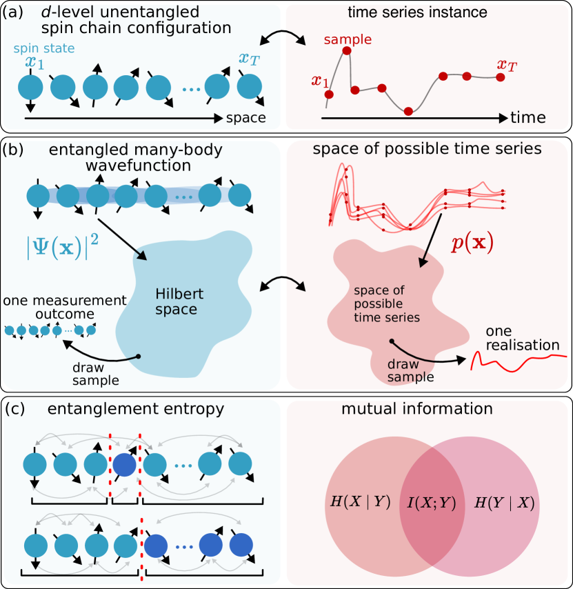
Figure 1: Mapping between quantitative formulations of quantum many-body physics and time-series analysis. Concepts in quantum physics (left, blue shading) and time-series analysis (right, red shading), and their associated theoretical and analytic tools, share similarities that motivate our MPS-based approach to time-series ML. (a) A $d$-level spin chain (left) exhibits one-dimensional (1D) spatial ordering, analogous to the 1D temporal ordering of time series, in which each sample is mapped to a discrete state which parallels that of an individual $d$-level quantum spin. (b) The probability density captured by the square of the wavefunction $|\Psi(\mathbf{x})|^{2}$ (left), is analogous to the joint probability density of a time-series process $p(\mathbf{x})$ (right). The wavefunction is a vector in an exponentially large Hilbert space, while time-series probability density is a distribution in the space of possible time series. A single measurement outcome (i.e., one spin chain configuration $\mathbf{x}$) governed by Born’s rule corresponds to sampling a single time-series realization (i.e., one time-series instance $\mathbf{x}$) from its generative distribution. (c) The entanglement entropy (left), which quantifies the degree of quantum entanglement between two spatial subsystems, is conceptually related to classical quantities such as the mutual information between temporal segments (right), both capturing statistical dependencies in their respective domains.

As we will show, for the purposes of time-series analysis, it is advantageous to view a $T$-sample time-series instance $\mathbf{x}=(x_{1},x_{2},\dots,x_{T})$ as a specific configuration of a $T$-body system, where each temporal observation $x_{t}$ – originally real-valued and continuous – is mapped to a discrete state $s_{t}$. Throughout the text, we refer to a single temporal observation $x_{t}$ as a time-series amplitude or time-series value. Here, analogous to a quantum many-body system, the wavefunction $\Psi(x_{1},x_{2},\dots,x_{T})$ encodes the joint distribution of time-series data, and is determined by the properties of the underlying generative process. Analogous ideas in quantum many-body physics and time-series machine learning are illustrated in Fig. 1. We emphasize that the joint probability distribution encompasses not just the empirical distribution of the observed time-series, but the full generative distribution from which individual time-series instances are sampled. In other words, each time-series instance $\mathbf{x}$ of $T$ measurements serves as a point sample from a $T$-dimensional distribution. As with its quantum analogue, within our MPS formalism for ML the probability density of observing a time-series instance $\mathbf{x}$ from the distribution encoded by $\Psi$ is given by Born’s rule:

$$p(\mathbf{x})=\lvert\Psi(\mathbf{x})\rvert^{2}\,.$$ (1)

Although such a wavefunction is exponentially large in general, it may be approximated by a $T$-site MPS ansatz [4] which provides a compressed tensor network representation:

$$W_{s_{1},...,s_{T}}=\sum_{\bm{\alpha}}A_{\alpha_{1}}^{s_{1}}A_{\alpha_{1},\alpha_{2}}^{s_{2}}\dots A_{\alpha_{T-2},\alpha_{T-1}}^{s_{T-1}}A_{\alpha_{T-1}}^{s_{T}}\,.$$ (2)

Here, $W$ is the low-rank MPS approximation of the original wavefunction (which can also be expressed in tensor form), each site $A^{s_{t}}$ corresponds to a measured point in time $x_{t}$, and the dimension of the bond indices $\bm{\alpha}=\{\alpha_{1},\ldots,\alpha_{T-1}\}$ may be adjusted to tune the maximum complexity of the MPS ansatz. Crucially, by compressing the wavefunction, and by extension, the joint distribution it encodes, the MPS approximation offers an explicit and tractable model of the generative distribution underlying time-series data. The ability to work directly with a tractable model of the full time-series joint distribution – rather than relying solely on the empirical distribution of observations – is what underpins the key innovations of our present work on MPS-based algorithms for time-series analysis. In particular, we show how inferring a joint distribution of time series with MPS, analogous to the distribution encoded by the quantum many-body wavefunction, allows us to tackle important statistical learning problem classes, including classification and imputation.

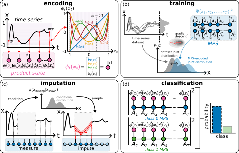
Figure 2: Time-series machine learning with MPS. (a) Each Real-valued time series amplitude $x_{t}$ is encoded in a $d$-dimensional vector $\phi_{t}$ by projecting its value onto a truncated orthonormal basis with $d$ basis functions. An entire time series (of length $T$ samples) is then encoded as a set of $T$ $\phi_{t}$ vectors, which we represent as a product state embedded in a $d^{T}$ dimensional Hilbert space. (b) Using observed time-series from a dataset, a generally entangled MPS – depicted here using Penrose graphical notation – with maximum bond dimension $\chi_{\rm{max}}$ is trained with a DMRG-inspired sweeping optimization algorithm to approximate the underlying joint distribution of the data. Two copies of the trained MPS (one conjugate-transposed, denoted by the dagger $\dagger$) with open physical indices encodes the learned distribution, allowing us to sample from and do inference with complex high-dimensional distributions in a tractable manner. In this work, we introduce MPS-based learning algorithms for two important time-series ML problems: (c) imputation (inferring unmeasured values of a time series), and (d) classification (inferring a time-series class). (c) Generative time-series modeling: we use conditional sampling to perform imputation of missing datapoints. Known points of a time series (black lines) project the MPS into a subspace, which is then used to find the unknown datapoints (red line). The same method can be used to tackle some forecasting problems if the missing points are future values. (d) MPS for classification: multiple labeled classes of time series are used to train MPSs. Taking the overlap of unlabeled time-series data (encoded as a product state) with each MPS determines its class.

II.1 Encoding time series as product states

The MPS ansatz is a powerful tool for compressing functions in an exponentially large Hilbert space. To leverage the MPS formalism to represent the joint probability distribution of a time-series process, we must map the continuous-valued time-series amplitudes, $x_{t}$, to vectors in a finite-dimensional Hilbert space, to make the time-series data compatible with the MPS formalism. To achieve this, we employ $d$-dimensional nonlinear feature maps, which throughout the text we refer to as the encoding:

$$\phi_{t}(x_{t})=[b_{1}(x_{t}),b_{2}(x_{t}),\ldots,b_{d}(x_{t})]_{t}\,,$$ (3)

which for a given choice of real or complex basis functions $b_{i}$, map a real valued time-series amplitude $x_{t}$ to a vector in $\mathbb{R}^{d}$ or $\mathbb{C}^{d}$. This mapping via the encoding $\phi_{t}(x_{t})$ is depicted schematically in Fig. 2(a). In general, the choice of basis functions $[b_{1},\ldots,b_{d}]_{t}$ can be time dependent, but here we consider a time-independent feature map. When applied to an entire time series of $T$ samples, the complete feature map $\Phi(\mathbf{x})$ is then given by the tensor product of local feature maps:

$$\Phi(\mathbf{x})=\phi_{1}(x_{1})\otimes\phi_{2}(x_{2})\otimes\ldots\otimes\phi_{T}(x_{T})\,.$$ (4)

To ensure the probabilistic interpretation of the wavefunction parameterized by the the matrix product state $W$ in Eq. (2) remains valid, the normalization condition:

$$\int_{x}|\Phi(\mathbf{x})\cdot W|^{2}{\mathrm{d}}\mu(x)=1\,,$$ (5)

must be satisfied [15]. This condition will hold, provided that: (i) the MPS is unitary; and (ii) the feature map is orthonormal under the measure $\mu(x)$ [20]. While many valid choices of feature map exist, including a Fourier basis, Laguerre and Hermite polynomials, in the present work we choose either $b_{i}(x)=P_{i}(x)$ or $b_{i}(x)=CF_{i}(x)$, the $i$th orthonormal Legendre polynomial, or $i$th complex Fourier basis function, respectively. In particular, the Legendre polynomials are well suited to encoding time-series data, as they satisfy the orthonormality conditions on the compact interval $[-1,1]$, and can generalize to any physical dimension $d$. Higher physical dimensions enable more complexity within each site and, when coupled with larger bond dimension, more complex the inter-site MPS interactions. This comes at the cost of increased computational storage and runtime.

To encode real-world time-series data using the Legendre basis, we first apply a pre-processing step to map the original values $\mathbf{x}\in\mathbb{R}$ to a compact domain $\mathbf{x}\in[-1,1]$. When using the MPS for time-series classification, we apply a scaled outlier-robust sigmoid transformation [36], before transforming the dataset to map the dataset minimum to $-1$, and the dataset maximum to 1 (min–max normalization). For imputation, preserving the shape of the data is essential, and care must be taken to ensure minimal distortion to imputed time-series when transforming between the encoding and original data domain. For this reason, we avoid nonlinear transformations (e.g., sigmoid transform), which can amplify encoding-related errors, particularly when mapping from $[-1,1]\rightarrow\mathbb{R}$. Rather, we only apply a linear min-max normalization. Further details about the specific data transformations used here are in Appendix A.

II.2 Training an MPS-based generative model

In the previous section, we laid the conceptual foundations for an MPS-based approach to time-series analysis. We motivated the MPS as being a powerful representation for encapsulating complex joint distributions underlying time series, and we described how we can represent time series in a form that is compatible with the MPS framework. In this section, we now outline the training procedure used to fit an MPS ansatz to a joint probability distribution given a finite training set of time series sampled from it. As we will show, the resulting MPS can be used to solve time-series machine learning problems, such as imputation of missing data, generation of new data, and classification of unseen data within a unified, interpretable, and tractable framework.

II.2.1 Loss function for generative modeling

Given a dataset of $N$ time series, the goal of training is to learn an MPS model which closely approximates the joint probability distribution of the data, shown schematically in Fig. 2(b). Starting with a randomly initialized MPS, a common approach to training is to iteratively update the MPS entries by minimizing the Kullback–Leibler (KL) divergence [37, 20, 16, 38, 39], a measure of the discrepancy between the probability distribution $p(\mathbf{x})$ captured by the MPS, and the true distribution $q(\mathbf{x})$ that gave rise to the data:

$$D_{KL}=\int_{\mathbf{x}}q(\mathbf{x})\log{\frac{q(\mathbf{x})}{p(\mathbf{x})}}{\mathrm{d}}\mathbf{x}\,,$$ (6)

where the integral is over every possible configuration of $\mathbf{x}$. In practice, the true distribution $q$ is unknown, so it is common to minimize an averaged negative log-likelihood (NLL) loss function [20, 40, 21, 18],

$$\mathcal{L}_{G}=-\frac{1}{N}\sum_{n=1}^{N}\log{p(\mathbf{x}_{n})}\,.$$ (7)

This is equivalent to minimizing the KL divergence (up to a constant). Once the MPS is trained, the joint probability density $p$ is extracted from the MPS using the Born rule, which now takes the form,

$$p(\mathbf{x}_{n})=\lvert W\cdot\Phi(\mathbf{x}_{n})\rvert^{2}\,.$$ (8)

To extend training to a classification setting, we treat each class of time series as originating from a separate joint probability distribution. Given $L$ classes of data, we need to learn $L$ probability distributions using $L$ separate MPSs. As in Stoudenmire and Schwab [15], an equivalent, yet more efficient approach is to attach an $L$-dimensional label index to a single site of an MPS:

$$W^{l}_{s_{1},...,s_{T}}=\sum_{\bm{\alpha}}A_{\alpha_{1}}^{s_{1}}A_{\alpha_{1},\alpha_{2}}^{s_{2}}\ldots A^{l,s_{j}}_{\alpha_{j-1},\alpha_{j}}\ldots A_{\alpha_{T-1}}^{s_{T}}\,,$$ (9)

and minimize the sum of the losses across every class:

$$\mathcal{L}=-\frac{1}{N}\sum_{n=1}^{N}\sum_{l=1}^{L}\log{\lvert W^{l}\cdot\Phi(\mathbf{x}_{n})\rvert^{2}}\,.$$ (10)

This allows us to approach generative modeling and classification in a unified manner, as the total loss $\mathcal{L}$ reduces to Eq. (7) in the single class ‘unsupervised’ case. To avoid confusion about ‘class dependence’ in the generative modeling sections, we will drop the label index $l$ from our notation when it is one dimensional.

II.2.2 Sweeping optimization algorithm

In this section, we outline the local optimization algorithm we used to minimize $\mathcal{L}$, Eq. (10), on the training data. We use the same per-site DMRG-inspired sweeping algorithm in Stoudenmire and Schwab [15], but using a modified version of tangent-space gradient optimization (TSGO) [39] in the local tensor update step. Here, we present only the key algorithmic steps as a summary, and direct readers to Stoudenmire and Schwab [15] for a detailed treatment.

Starting with a randomly initialized MPS of $T$ sites, encoding dimension $d$, and uniform bond dimension $\chi_{\rm init}$.

1. Attach the label index $l$ to the rightmost site of the MPS, and place the MPS in left-canonical form [4].

2. Merge the rightmost pair of tensors in the MPS, $A^{l,s_{T}}_{\alpha_{T-1}}$ and $A^{s_{T-1}}_{\alpha_{T-1}\alpha_{T-2}}$, to form the bond tensor $\mathcal{B}$.

3. Holding the remaining $T-2$ tensors fixed, update $\mathcal{B}$ using a modified TSGO steepest descent rule:

   $$\mathcal{B}^{\prime}=\mathcal{B}-\eta\frac{\partial\mathcal{L}/\partial\mathcal{B}}{\left|\partial\mathcal{L}/\partial\mathcal{B}\right|}\,,$$ (11)

   where $\eta$ is the learning rate. Since $\mathcal{L}$ is not complex differentiable, we use (one-half times) the Wirtinger derivative [41] to compute $\frac{\partial\mathcal{L}}{\partial\mathcal{B}}$, thereby accommodating complex-valued encodings (e.g., Fourier basis) if required.

4. Normalize the updated bond tensor:

   $$\mathcal{B}^{\prime}\leftarrow\frac{\mathcal{B^{\prime}}}{\lvert{\mathcal{B^{\prime}}\rvert}}\,.$$ (12)

5. Decompose $\mathcal{B}^{\prime}$ back into two tensors by singular value decomposition (SVD), retaining at most $\chi_{\rm{max}}$ singular values. The number of retained singular values corresponds to the maximum bond dimension shared between the two updated sites. The left and right tensors of the SVD are chosen so that the label index moves along the MPS, and is part of the bond tensor $\mathcal{B}$ at every step.

6. Repeat steps 2-5 for each adjacent pair of remaining tensors, traversing from right-to-left, then from left-to-right, for a fixed number of iterations, or until convergence is achieved.

As in Stoudenmire and Schwab [15], we define one sweep of the MPS to be a ‘round-trip’, i.e., one backward and one forward pass through all tensors in the MPS.

II.3 Imputation

Many empirical time series contain segments of time for which values are missing (e.g., due to sensor drop-out) or contaminated (e.g., with artifacts). This complicates resulting analyses and, for many algorithms (such as classification or dimension-reduction), requires imputation, i.e., that the missing data be inferred (‘filled in’) from values that were observed [42, 43]. For example, in some astrophysical star surveys, periods of sensor downtime is inevitable as a result of essential operational procedures [44], leaving ‘gaps’ in the recorded light curves of stars during which no observations are made. Existing approaches to imputing missing values in time series range from filling them with a simple statistic of observed values (e.g., the mean of the full time series [45]), linearly interpolating across the missing data, to inferring missing values based on fitted linear models (e.g., autoregressive integrated moving average (ARIMA)), similarity-based methods (e.g., $k$-nearest neighbor imputation from a training set of data (K-NNI) [46]), and machine learning algorithms (e.g., generative adversarial networks (GANs) [47], variational auto-encoders (VAEs) [48]). In this work, we present a generative approach to time-series imputation by leveraging the data distribution encoded by the MPS $W$ (as in Eq. 2), summarized schematically in Fig. 3 using Penrose graphical notation [49]. Our imputation approach, shown schematically in Fig. 2(c), consists of two main steps: (i) conditioning the MPS on known values; and (ii) inferring missing values from the conditioned MPS. Here, we summarize the key algorithmic steps and refer the reader to Appendix D for full details.

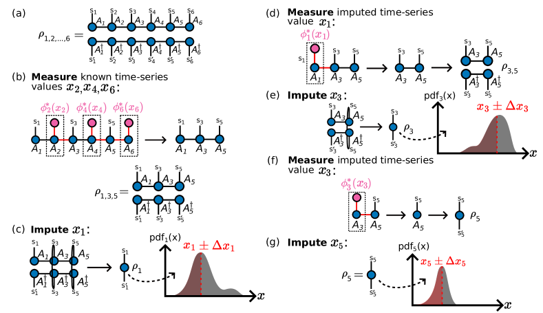
Figure 3: An MPS-based algorithm for time-series imputation. Here we consider an illustrative example of an imputation problem involving a six-site MPS, represented graphically with Penrose notation [49], where the time-series values $x_{2},x_{4},x_{6}$ are observed, and we would like to impute the unobserved values $x_{1},x_{3},x_{5}$. (a) Two copies of the trained MPS (one conjugate-transposed, indicated by the dagger, $\dagger$) with open physical indices encode the joint distribution over all possible states, given by $\rho_{1,2,\dots,6}$ (Eq. (14)). (b) The MPS is projected into a subspace where the states $s_{2}$, $s_{4}$, $s_{6}$, corresponding to each of the known time-series values, have been measured. The updated MPS now encodes the joint distribution over the remaining states $s_{1}$, $s_{3}$, $s_{5}$, conditional upon having measured $s_{2},s_{4},s_{6}$. (c) The single site conditional reduced density matrix $\rho$ (as in Eq. (15)) is obtained by tracing over all remaining sites. By evaluating the probability density function $\textrm{pdf}_{i}(x)=\phi_{i}^{\dagger}(x)\rho_{i}\phi_{i}(x)$ for $x$ in the encoding domain, we estimate the value for $x_{1}$ and its uncertainty $\Delta x_{1}$ using the median (see Eq. (17)) and weighted median absolute deviation (WMAD), respectively. (d) The MPS is projected onto the imputed state $s_{1}=\phi_{1}(x_{1})$ (Eq.(15)), yielding an updated MPS which encodes the joint distribution over $s_{3},s_{5}$. (e, f, g) We repeat estimating the next missing value using the median of the pdf (conditioned on all previously known and imputed values), then projecting the MPS onto the corresponding states, until all missing values are recovered.

Let the ordered sequence $\mathbf{x}^{*}=x_{1},x_{2},\ldots,x_{T}$ represent a time series with known observations $\{\mathbf{x}^{o}:o\in O\}$, and missing values $\{\mathbf{x}^{m}:m\in M\}$, where $M:=\{1,2,\ldots,T\}\setminus O$. The reduced density matrix for the unknown states $\rho_{M}$ can be obtained by first projecting the observed states onto the MPS:

$$\widetilde{W}_{s_{m_{1}},s_{m_{2}},\ldots}=W_{s_{1},...,s_{T}}\cdot\prod_{i\in O}\frac{\phi_{i}^{s_{i}\dagger}(x_{i})}{\sqrt{P(x_{i})}}\,,$$ (13)

and then taking the outer product:

$$\rho_{M}=\widetilde{W}\widetilde{W}^{\dagger}\,,$$ (14)

where $\widetilde{W}^{\dagger}$ is the conjugate transpose of $\widetilde{W}$. Throughout the text, we refer to the process of projecting the MPS onto a known value as either a measurement or conditioning a joint distribution on a known value. The scale factors $\sqrt{P(x_{i})}$ ensure that the MPS remains correctly normalized. Technical details of the implementation are described fully in Appendix D.

An important feature of MPS-based imputation is that each missing value is imputed one at a time, using both known observations and already imputed values that were previously missing. Therefore, the outcome of an imputation depends on the order in which it is performed. Time series are ordered in time, so we elect to perform imputation sequentially from earliest to latest using the ‘chain rule’ of probability, as described in [50]. While previous approaches typically sample a random state from the single-site conditional distributions (e.g., via inverse transform sampling [20]), here we use a deterministic approach wherein we select the state that corresponds to the median of the conditional distribution at each imputation site. Our choice to use the median is motivated by the fact that discretizing continuous time-series values using a finite number of basis functions $d$ artificially broadens the probability distribution. Sampling directly from this broadened distribution can artificially lead to outlying values being chosen which degrades the imputation performance. As detailed in Appendix B, selecting the median of the distribution effectively mitigates this broadening effect and provides a single best estimate for each imputation site. In what follows, we present our MPS-based algorithm for time-series imputation, recapitulated in Fig. 3. Starting at the earliest missing site, $i$, in $M$:

1. Obtain the single-site reduced density matrix (RDM) for site $i$, $\rho_{i}$, by taking the partial trace over all remaining (unmeasured) sites except for site $i$:

   $$\rho_{i}=\operatorname{Tr}_{M\setminus\{i\}}\left(\rho_{M}\right)=\operatorname{Tr}_{M\setminus\{i\}}\left(\widetilde{W}\widetilde{W}^{\dagger}\right)\,,$$ (15)

   where $\widetilde{W}$ is the projected MPS incorporating the observed states and $\rho_{M}$ is its corresponding density matrix as in Eq. (14).

2. Using the RDM, compute the cumulative distribution function $F_{i}(x)$ as

   $$F_{i}(x)=\frac{1}{Z}\int_{-1}^{x}\phi_{i}^{\dagger}(x^{\prime})\rho_{i}\phi_{i}(x^{\prime}){\mathrm{d}}x^{\prime}\,,$$ (16)

   with normalization factor $Z$ chosen so that $F_{i}(1)=1$.

3. Infer $x^{*}_{i}$ using the median of the conditional distribution

   $$x^{*}_{i}=\operatorname*{arg\,min}_{x}\left|F_{i}(x)-\frac{1}{2}\right|\,.$$ (17)

4. Project the MPS onto the selected state $s_{i}$ by contracting the MPS with $\phi_{i}^{\dagger}(x_{i}^{*})$, as in Eq. (13):

   $$\widetilde{W}^{\prime}=\widetilde{W}\cdot\frac{\phi_{i}^{\dagger}(x^{*}_{i})}{\sqrt{P(x^{*}_{i})}}\,.$$ (18)

5. Proceed to the next unknown time point and repeat steps 1–4 using the lower-rank MPS $\widetilde{W}^{\prime}$ until all missing values $\mathbf{x}^{m}$ are recovered.

II.4 Classification

Having established the theoretical foundations for training an MPS to learn a generative distribution underlying an observed time-series dataset, here we show how our framework can be naturally extended to the supervised setting to address the problem of time-series classification – the second key application of our approach. Specifically, for a dataset of time-series instances, each associated with a distinct class label $l$ from a finite set of classes $L$, the primary objective is to learn a model that can accurately predict the class label $l\in L$ of new, unseen time series by leveraging the learned generative distributions of the classes.

As stated in Sec. II.2, classification is achieved by training $L$ distinct MPSs. For each class, indexed by $l$, we train a separate MPS $W$ on the subset of time-series instances belonging to $l$. To classify an unlabeled time series $\mathbf{x}$, we then compute its (non-normalized) probability density $p(\mathbf{x})$ under each of the $L$ MPSs, and select the label $l$ of the MPS that assigns the highest relative probability to the instance, as illustrated schematically in Fig. 2(d).

In practice, the MPS formalism allows for a more efficient solution: by attaching an $L$-dimensional label index to a single MPS (at any site), we can train a unified model $W^{l}$ to simultaneously encode the generative distributions for all classes. For any time series $\mathbf{x}$, encoded as a product state $\Phi(\mathbf{x})$, we can then define the contraction:

$$f^{l}(\mathbf{x})=W^{l}\cdot\Phi(\mathbf{x})\,,$$ (19)

where the model output $f^{l}(\mathbf{x})$ is a length $L$ vector, with each entry being the similarity (overlap) between $\mathbf{x}$ and class $l$. To obtain the probability of $\mathbf{x}$ belonging to each class, we take the squared-norm of the output vector in order to satisfy the Born rule:

$$p(\mathbf{x}\mid l)=|f^{l}(\mathbf{x})|^{2}\,.$$ (20)

Since all classes are assumed to have the same prior probability $p(l)$, the probability of each class, given an unlabeled time series, $p(l\mid\mathbf{x})$, is directly proportional to its non-normalized likelihood $p(\mathbf{x}\mid l)$ i.e., $p(l\mid\mathbf{x})\propto p(\mathbf{x}\mid l)$ according to Bayes’ rule. Therefore, the predicted class can be determined directly from the model output by selecting the index $l$ corresponding to the largest entry in $f^{l}(\mathbf{x})$:

$$\operatorname*{arg\,max}_{l}|f^{l}(\mathbf{x})|^{2}\,.$$ (21)

In this section, we have introduced an MPS-based algorithm for learning a generative distribution underlying an observed time-series dataset. By leveraging the properties of the MPS to encode a tractable representation of complex joint distributions, it is possible to sample from and do inference on those distributions, unlocking the potential to tackle a wide range of important time-series analysis problems. Crucially, our approach allows us to perform these tasks, including imputation and classification, under a unified and statistically grounded framework.

III Numerical Experiments

In Sec. II above, we introduced a practical algorithm for learning an underlying probabilistic model from a time-series dataset, detailing how the encoded generative distribution can then be used as the basis of new MPS-based algorithms for time-series analysis tasks. While existing methods have been developed to address time-series ML tasks, such as classification and imputation independently, our approach is the first to tackle these problems within a common modeling framework by leveraging a tractable form of the complex joint distribution underlying time series. In this section, we aim to investigate the utility of MPSTime in a range of important data-driven problems involving synthetic and real-world time-series datasets. First, in Sec. III.1, we detail the construction of the datasets we investigate in our numerical experiments. Then, in Sec. III.2, we empirically validate our framework for MPS-based imputation on a synthetic dataset, showing that MPSTime can successfully learn the underlying joint distribution directly from time-series data.

III.1 Time-series datasets

To evaluate our MPS-based algorithm for time-series learning and inference, we investigated several synthetic and real-world datasets through a series of carefully constructed tasks. Here, we detail the pre-processing steps necessary to derive our classification and imputation tasks from publicly available time-series datasets. Table 1 provides a high-level overview of the datasets used in our experiments.

III.1.1 Synthetic datasets

We first aimed to validate the ability of MPSTime to infer distributions over time-series data by simulating time series from an analytic generative model. To this end, we investigated two synthetic test cases in which we simulated time series of length $T=100$ samples from a ‘noisy trendy sinusoid’ (NTS) model:

$$x_{t}=\sin{\left(\frac{2\pi}{\tau}t+\psi\right)}+\frac{mt}{T}+\sigma n_{t}\,,$$ (22)

where $x_{t}$ is the observed value at time $t\in[0,T]$, $\tau$ is the period, $m$ is the slope of a linear trend, $\psi\in[0,2\pi)$ is the phase offset, $\sigma$ is the noise scale, and $n_{t}\sim\mathcal{N}(0,1)$ are i.i.d. normally distributed random variables. A time-series dataset can be constructed by repeatedly generating time series from Eq. (22). The diversity of the time-series dataset (and thus complexity of the joint distribution over time series) can be controlled via the parameters of Eq. 22 that are fixed for all time series in the dataset, versus the parameters that are allowed to vary across the dataset. Here we analyzed six NTS datasets of differing complexity, generated through different such choices, as detailed below:

1. Simple settings: In our first test case, we fixed the period ($\tau=20$) and trend ($m=3$), while allowing the phase offset $\psi$ to vary across the time-series dataset. This was achieved by sampling a value for $\psi$ for each time series as a random sample from a uniform distribution, as $\psi\sim U(0,2\pi)$. We generated two training datasets containing $300$ time series each: one with: (i) NTS1, with low noise ($\sigma=0.1$); and (ii) NTS2, with moderate noise ($\sigma=0.2$). For imputation, we then generated a test dataset containing 200 time series on which to evaluate model performance.

2. Challenging settings: To simulate time series exhibiting richer dynamical variation, and therefore, more complex data distributions, we systematically expanded the parameter space of the NTS model. Fixing the noise scale at $\sigma=0.1$, we constructed four datasets with progressively more complex joint distributions by varying the trend $m$ and period $\tau$ parameters: (i) NTS3, with a single trend ($m=20$) and three periods ($\tau\in\{20,30,40\}$); (ii) NTS4, with three trends ($m\in\{-3,0,3\}$) and a single period ($\tau=20$); (iii) NTS5 with two trends ($m\in\{-3,3\}$) and two periods ($\tau\in\{20,40\}$); and (iv) NTS6, with three trends ($m\in\{-3,0,3\}$) and three periods ($\tau\in\{20,30,40\}$). In all cases, the phase offset $\psi$ was drawn randomly from a uniform distribution $\psi\sim U(0,2\pi)$, and the free parameter(s) were selected from randomly from the set of allowed values. In each case, we generated a training dataset of length $600$ time series to adequately sample the larger model parameter space. In each case, model performance was evaluated on a subsequent test set of $300$ generated time series.

III.1.2 Real-world datasets

We selected three real-world time-series datasets to analyze, representative of three key application domains: (i) medicine, (ii) energy, and (iii) astronomy:

1. ECG: Our medical dataset, ECG200 [51], is a two-class dataset of time series representing electrocardiogram (ECG) traces of single heart beats, labeled according to whether the signal originated from a healthy or diseased (myocardial infarction) patient. The problem is well studied in the time-series classification (TSC) literature. The dataset comprises 100 training instances and 100 test instances, where each time series contains $T=96$ samples. Of the $200$ total time series, $133$ ($66.5\%$) are labeled as ‘healthy’, and the remaining 67 ($33.5\%$) are labeled as ‘abnormal’. For classification and imputation tasks, we used the same open dataset published in the UCR time-series classification archive [52]. However, for imputation, we discarded label information and effectively treat all instances as belonging to the same data distribution (i.e., a single ‘class’).

2. Power Demand: ItalyPowerDemand [53] is a two-class dataset of time series corresponding to one day of electrical power demand in a small Italian city, sampled at 1-hour intervals, with each time series assigned to either ‘winter’ (recorded between October and March) or ‘summer’ (recorded between April and September). The dataset is split into $67$ training instances and $1029$ test instances, each of length $T=24$ samples. Of the total $1096$ time series, 547 (49.9%) are labeled as ‘winter’ (class 0) and the remaining 549 (50.1%) are labeled as ‘summer’ (class 1). For classification and imputation, we use the same open dataset published in the UCR time-series classification archive [52], omitting class labels for the latter task.

3. Astronomy: The KeplerLightCurves [54] dataset comprises $1319$ light curves from NASA’s Kepler mission. Individual time series correspond to stellar brightness measurements from a single star, sampled every $30$ minutes over a three-month quarter (‘Quarter 9’), yielding length $T=4767$ sample instances. For our classification task, we selected two of the seven classes that were particularly challenging to distinguish by eye: (i) non-variable stars, and (ii) $\delta$ Scuti stars. We then applied random under-sampling to the majority class to yield a balanced class distribution (201 non-variable stars and 201 $\delta$ Scuti stars). Instances were randomly assigned to either the train or test set using an 80/20 train/test ratio, and the first 100 samples of each time series were retained for classification.

   For the imputation task, we selected two classes from the KeplerLightCurves dataset: (i) RR Lyrae variable (25 time series), and (ii) non variable (25 time series). Unlike Power Demand and ECG, here we focused on the more typical imputation setting involving a single time-series instance. To construct the imputation datasets, each $T=4767$ sample time series was truncated to $4700$ samples and split into 47 non-overlapping windows of $T=100$ samples each. Windows containing true missing data gaps were discarded, and 80% of the remaining ‘clean’ windows (43 windows) were randomly allocated to the training set, with 20% (2 windows) allocated to the test set.

Table 1: Summary of all simulated and real-world time-series datasets analyzed here. Datasets are separated into those used for classification (labeled ‘C’) and imputation (labeled ‘I’) tasks, see Sec. III.1 for details.

Dataset	Train Size	Test Size	Length	Classes
ECG (C)	100 (50%)	100 (50%)	96	2
Power Demand (C)	67 (6%)	1029 (94%)	24	2
Astronomy (C)	321 (80%)	81 (20%)	100	2
NTS1–2 (I)§	300 (60%)	200 (40%)	100	1
NTS3–6 (I)	600 (67%)	300 (33%)	100	1
ECG (I)	100 (50%)	100 (50%)	96	1
Power Demand (I)	67 (6%)	1029 (94%)	24	1
Astronomy (I)‡	43 (96%)	2 (4%)	100	1

^§NTS1–2 refers to datasets NTS1 and NTS2. ^‡For Astronomy, we use ‘dataset’ to refer to the collection of fixed-length windows extracted from a single time-series instance. A total of 50 such datasets (i.e., 50 windowed time series) were evaluated.

III.2 Time-series imputation

So far, we have presented a practical and statistically grounded framework for MPS-based probabilistic modeling of time-series data. While the theoretical foundations are well-established, the practical efficacy of our approach – particularly the capacity to learn complex joint distributions for time-series ML problems – remains to be demonstrated. To bridge this gap between theory and practice, we now turn to an experimental validation of our approach, demonstrating first the ability of MPS to model complex joint distributions, and second, leveraging these learned distributions to perform an accurate imputation of missing values.

We begin by validating our approach on a relatively simple joint distribution of trendy sinusoids, providing a compelling proof-of-concept for the effectiveness of MPS-based imputation in a controlled setting. By systematically varying the parameters of our synthetic data generative model, we then show that a sufficiently expressive MPS can capture increasingly complex joint distributions of time-series data. Moving beyond synthetic examples, we apply our approach to impute missing values in three real-world datasets with unknown generative processes.

In order to demonstrate the performance of our MPS-based time-series imputation approach under varying degrees of data loss, we applied our method to several synthetic and real-world datasets. To simulate realistic scenarios often encountered in practical sensor deployments – such as sensor drop-outs due to misplacement, hardware failure, or data-downlinks – we focused on the contiguous missing data setting, where blocks of consecutive time-series observations were removed from test set instances. We note that if missing data are unmeasured future values, the imputation task can be considered a type of forecasting problem. Imputation performance was evaluated using the mean absolute error (MAE) defined as:

$$\text{MAE}=\frac{1}{n}\sum_{i=1}^{n}\lvert y_{i}-\hat{y}_{i}\rvert\,,$$ (23)

where $y_{i}$ is the actual missing value for the $i$-th data point, $\hat{y}_{i}$ is the imputed value for the $i$-th data point, and $n$ is the total number of missing values. A smaller MAE implies a higher accuracy.

To evaluate the imputation capabilities of our method, we varied the proportion of missing data points in each test instance by increasing the percentage of missing data from 5% to 95% of all samples. We then compared the imputation performance of our approach to several baselines, each selected to encompass a diverse range of approaches in the time-series imputation literature: (i) 1-Nearest Neighbor Imputation (1-NNI); (ii) Centroid Decomposition Recovery (CDRec); (iii) Bidirectional Recurrent Imputation for Time Series (BRITS); and, (iv) Conditional Score-based Diffusion Imputation (CSDI).

The classical baseline, 1-NNI [46], imputes missing data points by identifying the nearest neighbor in the training set (based on a Euclidean distance of observed samples), then substitutes the missing values with those from the neighboring time series. CDRec [55] decomposes a time-series matrix (i.e., an $N\times T$ matrix of $N$ time-series instances, each with fixed length $T$) into centroid patterns that capture recurring temporal behaviors, enabling the recovery of missing values through pattern-based reconstruction. The generative modeling baseline, CSDI, [56] uses a neural network-based diffusion model to gradually convert random noise into plausible imputed data points that are consistent with the data distribution conditioned on observed values. Finally, BRITS [57] is a popular deep learning method which leverages recurrent neural networks (RNNs) to model temporal dependencies in both forward and backward directions. While CDRec, CSDI, and BRITS were initially intended for multivariate time-series imputation, CDRec is one of the best performing algorithms in ‘total blackout’ scenarios [58], while CSDI is the best performing generative model-based imputation algorithm [42, 59], and most closely matches the distribution-learning approach of MPSTime.

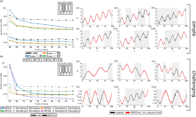
Figure 4: Time-series imputation of synthesized dataset. We compare MPSTime’s (solid line) imputation performance against the 1-nearest neighbor imputation (1-NNI) baseline (dotted line) on synthetic datasets of phase-randomized, noisy trendy sinusoids generated by the model defined in Eq. (22). The test-set mean absolute error (MAE) between the imputed values and ground-truth (unobserved) values is reported across varying percentages of missing data. (a) Simple setting: MPS with physical dimension $d=12$ and three different bond dimensions $\chi_{\rm{max}}=20,30,40$ (blue, orange, and green, respectively) trained on datasets with fixed trend $m$, fixed period $\tau$, and two noise levels $\sigma=0.1$ (NTS1, circle marker) and $\sigma=0.2$ (NTS2, diamond marker). (b) Challenging setting: MPS with $d=20$ and $\chi_{\rm{max}}=150$ trained on four datasets (NTS3-6) with increasingly complex underlying joint distributions, constructed by varying the trends $m$ and/or periods $\tau$ of noise-corrupted, phase-randomized sinusoids with $\sigma=0.1$, for the model defined in Eq. (22). In both (a) and (b), we show representative time-series examples of the MPS-imputed values on unseen (‘test’) time series generated from the same model [NTS2 dataset with $\chi_{\rm max}=30$ for (a) and NTS6 dataset with $\chi_{\rm max}=150$ for (b)] in the panels (ii)–(vii). The red shading represents the uncertainty, which here is quantified using the weighted median absolute deviation (WMAD).

III.2.1 Synthetic time series

Here, we investigate the ability of MPSTime to impute missing values from time-series data distributions of incrementally increasing complexity. Simulated instances were randomly split between training (60%) and testing (40%) sets. We varied the complexity of the dataset by changing the trend and period of the sinusoid, allowing us to systematically assess our method’s imputation performance across a range of challenging settings. Full details of the time-series model we used and its corresponding parameter values are in Sec. III.1.1.

For our simplest imputation setting, we examined two levels of additive Gaussian noise: (i) low noise ($\sigma=0.1$); and (ii) moderate noise ($\sigma=0.2$), where $\sigma$ denotes the standard deviation of the Gaussian noise distribution. In both cases, we held the period $\tau$ and trend $m$ fixed while allowing the phase to vary, which, for each time series, was drawn randomly from a uniform distribution, $\psi\sim U(0,2\pi)$. We then trained a $d=12$ MPS with three bond dimensions ($\chi_{\rm max}=20,30,40$) for ten sweeps on each of the training sets. For every test instance, we removed a central block of consecutive time-series points (with size determined by the percentage of total samples missing), maintaining approximately equal numbers of measured points on either side of the missing region.

Our first key result is presented in Fig. 4(a), and shows the MAE versus the percentage data missing. The relatively low MAE values demonstrate that an MPS can effectively learn the distribution underlying a finite number of time series, and using the learned distribution, can accurately impute missing values. As expected, imputation performance generally increased with the number of observed data points, as the MPS can leverage more conditioning information when the proportion of time-series samples that are observed increases. This effect does tend to saturate, however, as once the MPS gains enough information to determine the phase of the signal, apart from noise, it can then accurately approximate all other values. Six selected examples of the MPS-imputed time series for varying percentages of missing data are shown in subplots Figs 4(a)(ii)-(vii). Here, we also consider examples with multiple windows of missing data, which are not included in the evaluation presented in Fig. 4(a). In all cases, MPSTime could accurately infer the missing values. We observed that increasing the bond dimension $\chi_{\rm max}$ led to better imputation performance, with the most expressive MPS ($\chi_{\rm max}=40$) outperforming the 1-NNI baseline across all percentages of missing data, and for both noise levels. On the other hand, $\chi_{\rm max}=30$ performed similarly to $\chi_{\rm max}=40$ indicating that $\chi_{\rm max}=30$ is sufficiently expressive to learn the features of this dataset. We note that although there was an expected increase in MAE when increasing the noise level from $\sigma=0.1$ and $\sigma=0.2$, the $\chi_{\rm max}=30$ and $\chi_{\rm max}=40$ MPS could still accurately impute missing data when $<85\%$ of the data was missing. The imputation results here indicate that, for these bond dimensions, the MPS is sufficiently expressive to learn the joint probability distribution of the noisy sinusoid time series and can accurately impute missing values even when only a fraction of time-series values are observed.

Having demonstrated that our MPS framework can successfully encode the joint distribution underlying the simple trending sinusoidal dataset, we next aimed to test the ability of the MPS to model more complex synthetic time-series processes. To achieve this, we now use the more challenging setting and investigate several iterations of complexity by allowing the trend $m$ and/or the period $\tau$ to vary while holding the noise fixed at $\sigma=0.1$. We used the same train-test ratio as the simple dataset, however, this time training a $d=20,\chi_{\rm max}=150$ MPS for 10 sweeps. The larger value of $d$ was chosen to improve the resolution of the encoding for imputation, while the larger $\chi_{\rm max}$ value was chosen to allow the model to express the more complex correlations of the more challenging dataset. Figure 4(b) shows the mean imputation error versus the percentage of data missing across the four datasets, each with a different number of trends and periods. For almost all values, the MPS is able to outperform the 1-NNI baseline. We observe that for $<85\%$ of the data missing, the value of the MAE becomes largely fixed. This is similar to the simple dataset where, once a sufficient amount of the data is present, the projected MPS can determine the phase, period, and trend of the sinusoid and successfully fill in missing values. We note that the MPS performed best on the most complicated dataset, which contained three trends and periods. This is likely because of the large bond dimension $\chi_{\rm max}=150$ which is sufficiently expressive to learn the features of complex datasets, but can lead to overfitting on simpler ones. In addition to this, six selected examples for varying percentages of missing data are shown in subplots Figs 4(b)(ii)-(vii). All examples indicate successful imputation of missing data in the more challenging dataset.

In general, the results presented in Figs 4(a)-(b) demonstrate that the MPS framework can learn the joint probability distribution of a time-series process to a degree such that it can accurately infer the probabilistic model of trending sinusoidal functions. The successful imputation of the more complicated dataset indicates that the MPS is sufficiently expressive to encode the generative model of a process with varying period, trend and phase. This first successful result shows that MPS has significant potential as a time-series analysis tool for generative modeling of a broad class of datasets with complex correlation structures.

III.2.2 Real-world time series

Building on our demonstration of the imputation capabilities of the MPS, given synthetic time series from a known generative process, we now investigate its applicability to real-world time-series datasets. For our imputation tasks, we focused on time-series datasets from three domains of application to highlight the broad utility of our approach to: (i) medical data (the ‘ECG’ dataset); (ii) industrial data (the ‘Power Demand’ dataset), and (iii) astronomy (the ‘Astronomy’ dataset). To ensure that our imputation results were not biased by any particular train–test split, we adopted the dataset resampling strategy for time-series classification tasks in Bagnall et al. [60]. Specifically, we generated 30 resampled train-test splits for each dataset, then for each split we trained an MPS on the training set and evaluated its imputation error on instances from the test set, across various percentages of missing data. For any given percentage data missing, we imputed up to 15 randomly selected missing data block locations to account for the possibility that some regions may be easier to impute than others. Using the same folds and window locations for each dataset, we repeated the imputation experiment with the four baselines: 1-NNI, CSDI, BRITS, and CDRec. For demonstration purposes, we chose MPS hyperparameters that performed well on the first train-test split of each dataset based on a very simple grid search, and then held these values constant on the ‘unseen’ splits. For ECG and Power Demand, we trained a $d=10$, $\chi_{\rm max}=20$ MPS for 5 sweeps, and on the Astronomy dataset, we trained a $d=12$, $\chi_{\rm max}=35$ MPS for 3 sweeps. For the ECG and Power Demand datasets, we measured imputation performance with MAE, while the normalized MAE (NMAE) was used for the Astronomy dataset (due to differences in scale imposed by the individual windowing).

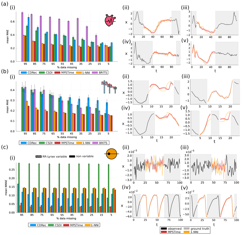
Figure 5: MPSTime demonstrates competitive and often superior performance for time-series imputation on real-world datasets. The window location and test set-averaged MAE and 95% CI across 30 folds is shown in subplot (i) as a function of percentage data missing for each dataset: (a) ECG, (b) Power Demand, (c) Astronomy. For ECG and Power Demand, we trained a $d=10$, $\chi_{\rm max}=20$ MPS, and for the Astronomy dataset, we trained a $d=12,\chi_{\rm max}=35$ MPS. For each dataset, in panels (ii-v), we show representative examples of the MPS-imputed time-series (solid red line) and uncertainty due to encoding error (shaded ribbons) alongside the 1-NNI baseline (solid gold line). The shaded windows correspond to segments of observed time-series values, while the transparent windows correspond to missing data blocks. The ground-truth (unobserved) time-series values (gray line) are plotted for comparison with the imputed values.

The imputation performance of the MPS relative to the various baselines is shown in Fig. 5(a)-(c) for the ECG, Power Demand, and Astronomy datasets respectively. Starting with the ECG dataset, Fig. 5(a)(i) shows the mean MAE versus the percentage of data missing in the imputation. We observe that the MPS has superior performance to other baselines for all values of data missing. As with the synthetic data, once a sufficient number of data points are present, in this case $<85\%$ missing, the performance of the MPS maximizes and saturates. Again, this indicates that with MPS is able to lock on to the signal once a sufficient amount of information is present. Figures 5(a)(ii)–(v) show selected examples of imputation performed for different window sizes and positions in the ECG dataset. Here, we emphasize that the functional form of the ECG dataset is highly nonlinear and more complex than the synthetic datasets presented in the previous subsection. Nevertheless, the MPS framework can still learn a joint probability distribution of the dataset to a sufficient degree that it can accurately impute missing data points with only a fraction of data being present.

Figure 5(b)(i) shows the imputation results for the Power Demand dataset. This dataset is shorter than previous examples and with 24 samples in each series. Again, the MPS showed superior performance to all other methods tested, and could accurately impute missing points. As with previous results, the performance of the MPS tended to saturate when $<85\%$ of the data was missing, again indicating that the MPS framework can learn the trend of the time series with very few conditioning points. This is in contrast to other methods such as CSDI and BRITS whose performance was competitive with the MPS when $5\%$ of the data was missing, but degraded significantly when larger fractions of the data were missing. Figure 5(b)(ii)-(v) show four selected examples of imputation in the Power Demand dataset with different configurations of missing data.

Finally, Fig. 5(c)(i) shows the imputation performance for the Astronomy dataset. Here the performance is split between the RR-Lyrae variable instances and the non variable instances. This is because, as seen in the examples in Fig. 5(c)(ii)-(v) these two sets of time series have very different properties with the RR-Lyrae variable being almost perfectly periodic, while the non variable time series are not. Here, the 1-NNI baseline showed superior performance for the RR-Lyrae variable data. This is not unexpected due to the periodic nature of the time series in this dataset. Since the 1-NNI method finds a sample from the training data that is closest to the data that is being imputed, for periodic datasets, there is a high probability that the training data contains a time series that is very close to the one being imputed. On the non-variable dataset CDRec outperformed MPSTime, although here, MPS performed better than CSDI and 1-NNI. Unlike the previous examples, the performance of the MPS did not show a significant performance improvement with less data missing, or a saturation effect after a fixed number of data points were known. This was particularly visible for the non variable dataset, which showed approximately constant MAE for different fractions of data missing.

The imputation results presented for real-world datasets in Fig. 5 show that MPSTime can learn joint probability distributions of challenging, highly nonlinear functions that arise in real-world time series. A notable aspect of the MPS performance was that, for the ECG and Power Demand datasets, the joint probability distribution was learned with a sufficient degree of accuracy that when $<85\%$ of the data was missing, MPSTime could perform imputation with a MAE value of $<0.3$ for ECG and $<0.2$ for Power Demand. For these datasets, MPSTime outperformed all other methods. Although the MPS method did not outperform in the Kepler dataset, overall, its performance was among the best in all the imputation tests we performed. The results in Fig. 5 highlight that we can learn complex joint probability distributions that underlie real-world time-series processes well enough to perform accurate imputation. MPSTime therefore offers a very promising approach for performing imputation on a diverse array of real-world time-series datasets for a range of applications.

III.3 Time-series classification

Having shown that MPSTime can accurately impute missing values in a range of challenging scenarios, including those involving real-world datasets, we now demonstrate its ability to infer data classes through a series of time-series classification (TSC) tasks. To underscore the inherent versatility of MPSTime in addressing diverse ML objectives within a unified framework, we constructed classification tasks from the same open datasets that seeded the real-world imputation experiments in Sec. III.2 and detailed in Sec. III.1.

For each TSC task, we compare the performance of MPSTime to three baselines, each selected to represent a distinct algorithmic paradigm within the TSC literature. Our selection of baselines comprises: (i) Nearest Neighbor with Dynamic Time Warping (1-NN-DTW) [60]; (ii) InceptionTime [61]; and (iii) HIVE-COTE V2.0 (HC2) [62]. The classical elastic distance-based classifier, 1-NN-DTW, is a standard benchmark against which many new algorithms are compared, given its strong performance across various TSC problems on the UCR repository [60]. At the time of constructing our classification tasks, InceptionTime was considered best in category for deep learning [63]. While a recent variant, H-InceptionTime [64], has shown small but significant improvements in classification accuracy over the original InceptionTime algorithm [63], to the best of our knowledge, there are no readily available implementations for this variant. Finally, HC2 is a meta-ensemble of classifiers, each built on different time-series data representations (e.g., shapelets, bag-of-words based dictionaries, among others). Recent benchmarking studies have placed HC2 as the current top-performing algorithm for TSC, evaluated across all datasets in the UCR repository [63]. Further discussion about the TSC baselines is provided in Appendix G. We emphasize that our selection of HC2 and InceptionTime as TSC baselines – both highly expressive and computationally intensive – establishes an especially challenging setting in which to compare the performance of MPSTime.

To benchmark MPSTime against the various baselines, we evaluated classification accuracy using cross-validation across 30 stratified train-test resamples, as per Middlehurst et al. [63]. For the ECG and Power Demand datasets, we used the original train-test split published on the UCR repository as the first fold, and generated 29 additional folds using reproducible random seeds. For these datasets, we report the published 30-fold classification accuracy results for the baselines (available at the UCR repository [52]).

As the Astronomy dataset was derived as a two-class subset of the standard KeplerLightCurves open dataset (see Sec. III.1.2), published results are not publicly available for the baselines. Therefore, we evaluated reference implementations of 1NN-DTW, InceptionTime and HC2 on the Astronomy dataset, following the same 30-fold train-test resample approach outlined above. Training details, including hyperparameter settings and specific implementations for the baselines, are in Appendix G. For MPSTime, we chose parameters that performed well in our preliminary experiments on the Astronomy dataset. We note that this particular choice does not confer an unfair advantage: the 30-fold resampling methodology safeguards against configuration bias, as superior performance must be demonstrated consistently across multiple evaluation contexts (i.e., different train-test splits), rather than relying on fold-specific optimizations that may not generalize.

The classification results, shown in Fig. 6, highlight the strong performance of MPSTime, which achieves TSC accuracies competitive with state-of-the-art ML methods on our benchmarks. Notably, for both ECG and Power Demand datasets, MPSTime achieves accuracies that closely match (within statistical uncertainty) the top-performing deep learning and ensemble methods, InceptionTime and HC2, respectively, while outperforming the classic 1-NN-DTW benchmark on these benchmarks. On the Astronomy dataset, we observed the greatest variability in performance differences across different methods, with MPSTime achieving a mean accuracy of $0.91\pm 0.01$, which was lower than both InceptionTime ($0.93\pm 0.01$) and HC2 ($0.96\pm 0.01$). It is worth noting that with the Astronomy TSC task, we did not perform extensive hyperparameter tuning for MPSTime as for ECG and Power Demand. The baseline methods, while evaluated with default parameters, benefit from extensive prior optimization studies that inform these default configurations. A systematic exploration of MPSTime’s parameter space, comparable to those conducted for the baseline methods, could yield more competitive results for the Astronomy dataset.

Interestingly, for the ECG and Power Demand TSC tasks, hyperparameter tuning of MPSTime revealed optimal values of $d$ in the range of $3$-$6$, which is notably lower than those required for accurate imputation (in the range $d=10$–$12$) on the same datasets in Sec. III.2.2. On the other hand, optimal values of $\chi_{\rm max}$ were comparable across TSC ($\chi_{\rm max}=15$–$25$) and those yielding accurate performance on imputation tasks ($\chi_{\rm max}=20$) for these two datasets. These findings are consistent with the fundamental differences between classification and imputation tasks. In particular, we observe optimal classification performance with lower $d$ values (i.e., $d=3$-$6$) as the model only needs to learn the essential features that distinguish between classes. Optimal imputation demands a more expressive model and larger $d$ value (i.e., d in the range $10$-$12$) to accurately capture and do inference on the complex joint distribution underlying time-series datasets. This requirement stems from the discretization discussed in Sec. II.1: larger $d$ enables a finer-grained discretization of the originally continuous time-series values, which, leads to a more accurate approximation of the original time-series joint distribution. When doing inference on the encoded distribution, a higher $d$ thus allows for a more accurate reconstruction of missing values. In summary, our TSC experiments demonstrate that MPSTime achieves competitive classification performance on real-world time-series datasets when compared to state-of-the-art methods. These findings recapitulate the versatility of our approach in tackling multiple time-series ML objectives under a single framework.

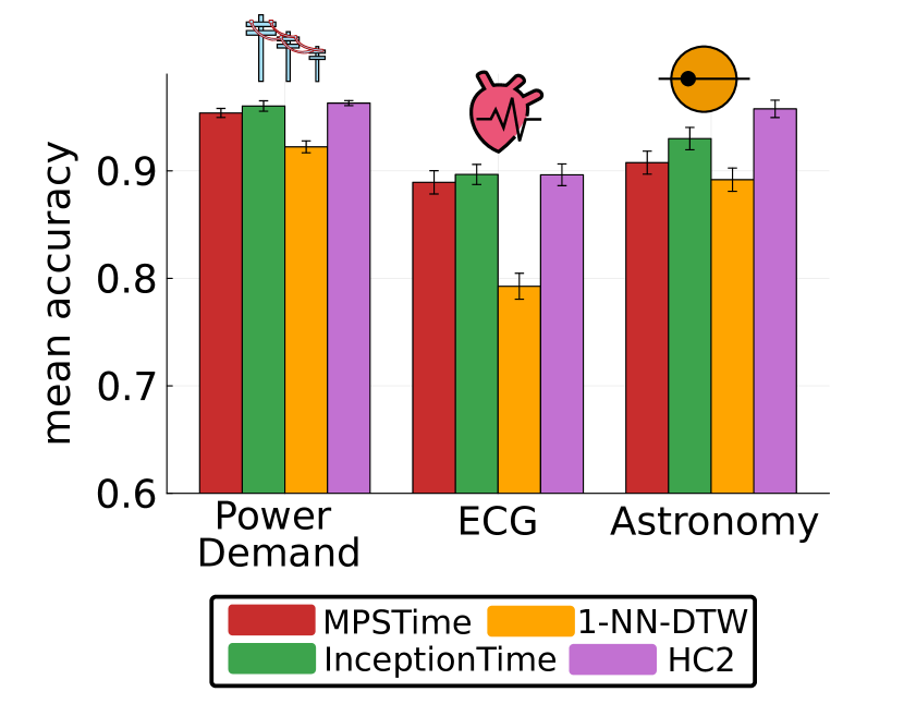
Figure 6: MPSTime outperforms a classic time-series classification benchmark (1-NN-DTW) and is competitive with modern state-of-the-art algorithms. The mean classification accuracy and 95% CI (across cross-validation folds) are shown for each of the three empirical datasets: Power Demand, ECG, and the Astronomy dataset. We compare our MPS classifier with three baselines: one nearest neighbor with Dynamic Time-Warping (1-NN-DTW), InceptionTime, and HIVE-COTE 2.0 (HC2).

IV MPS interpretability

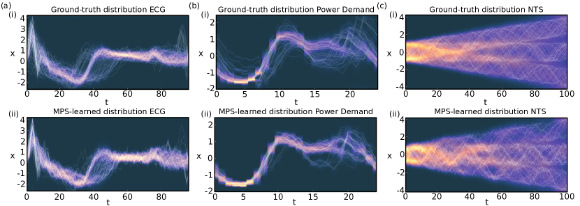
Figure 7: Sampling MPS joint probability distributions. At each time-point, the time-marginalized kernel density estimate (KDE) of time-series amplitudes is visualized as a heat map, overlaid with individual training instances for reference. For each dataset – (a) ECG, (b) Power Demand, and (c) the most complex Noisy, Trendy Sinusoid (NTS) dataset from Sec. III.2.1 with 3 periods and 3 trends – we show two panels: in subplot (i), we show the ground-truth training data, with the KDE heat map computed from the training instances and overlaid with examples of time series from the training set. Subplot (ii) shows the synthetic data generated by sampling from a $\chi_{\rm max}=80$, $d=12$ MPS trained on the corresponding dataset. Using inverse transform sampling, we generate each time-series amplitude conditionally from the MPS-encoded distribution, computing the KDE heat map from the synthetic dataset, and overlaying with representative examples of the synthetic single-shot trajectories.

A compelling justification for using MPS to infer complex joint time-series distributions directly from data lies in their inherent interpretability, which sets them apart from ‘black-box’ approaches. For example, the single-site reduced density matrix (RDM) $\rho$, as in Eq. 14, can be used to extract the learned conditional probability distribution of time-series amplitudes at a given time point $t$, directly from the MPS. If amplitudes of other sites are known, this can be used to constrain the distribution given by $\rho$ by conditioning other sites on their known values. As we have shown in Sec. III.2, the RDM forms the foundation of conditional site-wise sampling, enabling us to effectively impute missing values in time series by leveraging the temporal dependencies encoded by the MPS during training. Beyond its role in sampling, the RDM, which encapsulates all interactions between a given subsystem and the rest of the MPS, serves as a powerful tool for characterizing the local and global correlation structures captured within the model.

In this section, we harness analytical tools and machinery from quantum information theory to showcase the rich interpretability of MPSTime. Specifically, we demonstrate how these tools provide meaningful insights into the complex temporal correlations learned by the MPS. In Sec. IV.1, we study the generative distribution learned by the MPS through sampling entire time-series trajectories from the encoded joint distribution and comparing these to real-world instances from the training set. Through this qualitative investigation, we aim to determine whether the MPS is able to successfully capture complex temporal correlations from a finite number of training instances, and as a result, produce plausible synthetic data, as the sampling process explicitly relies on the temporal dependencies learned at each MPS site. In Sec. IV.2, we show how the complex correlations encoded by the MPS can be understood through the lens of entanglement entropy, extending fundamental concepts from quantum information theory – traditionally applied to analyze MPS in quantum many-body physics – to the analysis of temporal correlation structures learned by the MPS in a time-series ML setting.

IV.1 Unveiling temporal correlation structures learned by MPS through sampling

Building upon our earlier results in Sec. III.2, where we used partially observed time series to impute missing values from the conditional distribution represented by the MPS, we now study how accurately MPSTime can capture the joint time-series distribution from which a given time-series dataset is sampled. To this end, we generated single-shot trajectories (entire $T$-sample instances) directly from the MPS-encoded joint distribution. Unlike imputation, which begins with conditioning the MPS on partially observed time series, we randomly sample values directly from the unconditioned joint distribution using inverse transform sampling. The sampling process begins at the first MPS site, then proceeds sequentially from left-to-right, at each site, selecting a random state from the RDM, then updating the MPS to reflect the selected state, until all sites have been sampled once. This yields a single time-series instance of $T$ samples. By returning to the first site and sampling again, additional independent trajectories can be generated from the modeled joint distribution. A discussion of the specific inverse transform sampling method we use is given in Appendix E.

For our investigation, we focused on one synthetic (NTS6) and two empirical datasets (Power Demand and ECG). For the purposes of qualitative comparison, we selected values of $\chi_{\rm max}$ and $d$ that ensured the MPS possessed sufficient expressibility to model the essential temporal correlations (i.e., larger $\chi_{\rm max}$), while producing trajectories from the encoded generative distribution with small encoding error (i.e., larger $d$). To achieve this, we trained a $\chi_{\rm max}=85$ and $d=12$ MPS for all three datasets. From each MPS, we then generated the same number of trajectories as there were time-series instances in the training set, allowing for a direct comparison between realizations from the various modeled and original data distributions. In Fig. 7 we qualitatively compare the synthetically generated time-series instances from the MPS to training instances from the ground-truth joint distribution. In all cases, the MPS was able to replicate the data distribution underlying a finite number of time-series instances, as evidenced by its ability to generate new time-series that closely resemble the training data.

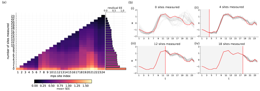
Figure 8: Interpreting the joint probability distribution of the MPS using the single-site entanglement entropy (SEE). By sequentially updating the MPS ($d=12$, $\chi_{\rm max}=80$) with each additional measured site, the SEE reveals how the entanglement in the remaining unmeasured sites evolves. This SEE structure provides insight into the contextual dependencies captured by the MPS, which, as it is conditioned on each additional site, reflects an evolving conditional distribution. Panel (a) shows the mean SEE across the Power Demand test set as a function of the number of sequentially measured sites (y-axis), starting from the first site and progressing from left (site 1) to right (site 24). The accompanying bar plot depicts the residual entanglement entropy – defined as the average unmeasured SEE – for varying numbers of measured sites. Panel (b) shows representative time-series trajectories sampled from the MPS for varying numbers of measured sites. These trajectories demonstrate how the conditional distribution of time-series amplitudes evolves as increasingly many points are measured: (i) no sites measured, (ii) 4 sites measured, (iii) 12 sites measured, (iv) 18 sites measured. The solid red line indicates the ground-truth time-series being used to condition the MPS.

IV.2 Conditional entanglement entropy

In a quantum mechanical system, the single-site entanglement entropy (SEE) quantifies the amount of entanglement shared between a single site and the remainder of the system [28]. When adapted to MPS-based time-series ML, the SEE determines the extent to which the time-series amplitude at a single site depends on the value of all other amplitudes (see Fig. 1(c)). If the SEE is large, this implies strong correlations with the remainder of the MPS, i.e., determining the amplitudes at other sites (time points) can reduce uncertainty about the amplitude at the site under consideration. On the other hand, a small SEE suggests the site behaves more independently, and therefore, determining the amplitudes of other sites does little to constrain its value through uncertainty reduction.

Examining how the SEE changes after conditioning on the time-series amplitude at one or more sites can therefore provide insight into the conditional relationships learned by the MPS. As a concrete example, consider an unmeasured site $B$ with $\textrm{SEE}_{\rm before}>0$. We then “measure” another site $A$, projecting the MPS onto a subspace in which the local state at $A$ is fixed to the observed time-series value. If this conditioning reduces the SEE at site $B$, i.e., $\textrm{SEE}_{\rm after}<\textrm{SEE}_{\rm before}$, this implies that $B$’s state is strongly influenced by knowledge of $A$’s state. In other words, observing a particular time-series amplitude $x_{A}$ at site $A$ constrains the distribution of amplitudes $x_{B}$ can take at site $B$. Extending this approach across multiple pairs or sets of sites can allow us to ‘map out’ more complex correlation structures encoded by the MPS.

For an MPS site $A_{i}$, the SEE is defined as the von Neumann entropy of the single-site reduced density matrix [65]:

$$S=-\sum_{k=1}^{r}\lambda_{k}\ln{\lambda_{k}}\,,$$ (24)

where $\lambda_{k}$ are the eigenvalues of the single-site reduced density matrix $\rho_{i}$ with rank $r$.

To showcase the insights facilitated by the SEE, we analyzed the same MPS trained on the Power Demand dataset in Sec. IV.1. For our analysis, we aimed to uncover the conditional dependencies learned by the MPS by observing how its entanglement structure evolves as increasingly many site-wise measurements are made. Here, we chose to perform measurements in a sequential order, starting at the first site and incrementing the number of measured sites by one. With each additional measurement, we analyzed the SEE of the remaining unmeasured sites in order to isolate the influence of the measurement on the resulting entanglement structure.

In Fig. 8(a)(i), we visualize the conditional entanglement structure of the MPS by averaging the measurement-dependent SEE over the entire Power Demand test set of $1029$ instances. As a proxy for the remaining entanglement encapsulated by the MPS after cumulative measurements, we also computed the residual entanglement entropy as the average SEE of the unmeasured sites. As expected, as more sites of the MPS are conditioned, the SEE decreases throughout the MPS. Interestingly, there appear to be key sites where, after they are conditioned, the SEE drops sharply. This occurs after measuring sites (correspond to time values in the MPS) 1, 2, 8, and 18. This indicates that the values at these points are likely crucial in determining the values of other points within the MPS. Figure 8(b) shows the sampled trajectories of the joint probability distribution learned by the MPS conditioned on 0-18 sites being measured with known amplitudes of a single time series. Moving from (i)-(iv) we clearly observe a reduction in the fluctuations in the trajectory amplitudes as more sites are measured. The reduction in fluctuations is particularly prominent between $t=15$ and $t=23$. This indicates that the conditional SEE can be used as a proxy for determining the certainty of the values of unmeasured sites conditioned on the measurement outcomes of other sites. The results illustrated in Fig. 8 highlight the utility of the MPSTime, which can be used to compute the conditional trajectories and conditional SEE. We emphasize that such calculations would be highly challenging or impossible to perform with the empirical dataset alone, while they are naturally extracted from the MPS framework.

V Discussion and Conclusion

Here we have presented MPSTime, an end-to-end framework for training and applying matrix-product states to time-series machine-learning problems. We show that a generative model parameterized by an MPS can effectively capture complex, high-dimensional joint time-series distributions, making it particularly well-suited to handling the challenges of time-series data. Leveraging the joint distribution encoded by the MPS, we demonstrate the versatility of our model by tackling important problems in time-series ML – imputation and classification – within a flexible and interpretable statistical framework. To our knowledge, this is the first framework for inferring joint distributions directly from time-series data. This provides a unified approach for tackling important problems, including classification, imputation, and synthetic data generation. Previously, existing approaches in the ML literature have treated these tasks in a disjoint manner, lacking a clear and common conceptual basis. Further, for the applications in this work, our MPS-based generative model only requires moderate bond dimension $\chi_{\rm max}$ and physical dimension $d$, striking a compelling balance between model expressiveness and computational efficiency.

In conclusion, we first validated our method on a range of synthetically generated datasets, showcasing its remarkable ability to recover missing data under diverse and challenging conditions. Our results underscore the model’s capacity to impute values in datasets with complex temporal correlations, achieving near-ground-truth accuracy even when faced with noisy and limited observations. We further benchmarked the method on three real-world datasets, where it demonstrated competitive and often superior performance relative to several classical and state-of-the-art imputation algorithms. Having demonstrated the promising imputation capabilities of the MPS, we then showcased its flexibility to adapt to classification tasks on the same real-world datasets. The MPS classifier exhibited robust performance across all three datasets, achieving mean classification accuracies comparable to those of state-of-the-art classification algorithms.

Appendix A Data pre-processing details

Here we discuss the details of the data transformations we applied to each raw time-series dataset prior to encoding them with the feature map. For a given time-series dataset of $N$ instances and $T$ data points (samples) per instance, represented by an $N\times T$ data matrix $\bm{X}$, the outlier-robust sigmoid transformation is given by [36]:

$$\bm{X^{\prime}}=\left(1+\exp{-\frac{\bm{X}-m_{\bm{X}}}{r_{\bm{X}}/1.35}}\right)^{-1},$$ (25)

where $\bm{X^{\prime}}$ is the normalized time-series data matrix, $\bm{X}$ is the un-normalized time-series data matrix, $m_{\bm{X}}$ is the median of $\bm{X}$ and $r_{\bm{X}}$ is its interquartile range. In the case of a scaled robust sigmoid transform, an additional linear transformation, commonly referred to as MinMax, is applied to $\bm{X^{\prime}}$ such to rescale it to the target range $[a,b]$:

$$\bm{X^{\prime\prime}}=\left(b-a\right)\cdot\frac{\bm{X^{\prime}}-x^{\prime}_{\text{min}}}{x^{\prime}_{\text{max}}-x^{\prime}_{\text{min}}}+a,$$ (26)

where $\bm{X^{\prime\prime}}$ is the scaled robust-sigmoid transformed data matrix, $x^{\prime}_{\text{min}}$ and $x^{\prime}_{\text{max}}$ are the minimum and maximum of $\bm{X^{\prime}}$, respectively. In cases where we only apply the linear rescaling, we use the same transformation in Eq. 26, but applied to the raw data matrix $\bm{X}$ rather than the sigmoid transformed data matrix $\bm{X^{\prime}}$.

When we evaluated a trained model on unseen data, the unseen data was preprocessed with the values $m_{\bm{X}}$, $r_{\bm{X}}$, $x^{\prime}_{\text{min}}$, and $x^{\prime}_{\text{max}}$ extracted from the training dataset. An undesirable implication of this is that occasionally test time series were preprocessed to map outside of the range $[a,b]$. For each of these time-series instances:

1. If the minimum was less than $a$, the time series was shifted up so it had a minimum value of $a$.

2. After that, if the maximum was larger than $b$, the time series was rescaled so it was at most $b$.

These outliers had no meaningful bearing on the results. For example, for the default UCR train/test split of the ECG dataset, only $5$ out of the $100$ time series in the test set were shifted up by $0.1\%$, $0.1\%$, $0.2\%$, $1\%$, and $1.7\%$, respectively. No time series were rescaled. For the default UCR train/test split of the Power Demand dataset, only $34$ out of the $1029$ test time series were altered: $13$ were shifted up, the five largest shifts were: $1.9\%$, $2.1\%$, $2.1\%$, $4.4\%$ and $5.1\%$. A total of $23$ time series were rescaled, with the five largest rescales being by $2.6\%$, $3.0\%$, $4.1\%$, $4.5\%$ and $8.8\%$.

When evaluating imputation performance in Sec. III.2, the mean absolute error (Eq. (23)) was computed on the raw (non-preprocessed) data.

Appendix B Impact of artificial broadening from finite basis representation on conditional imputation

In this work, we train an MPS to encode a probability distribution of time-series amplitudes. As these amplitudes are originally real-valued and continuous ($x_{t}\in\mathcal{R}$), they must first be mapped to discrete quantum states ($\ket{x_{t}}$) to be compatible with the MPS framework. To achieve this discretization, we project the amplitudes onto a truncated basis set of $d$ functions, $\phi_{t}(x_{t})=\{b_{1}(x_{t}),b_{2}(x_{t}),\ldots,b_{d}(x_{t})\}_{t}$. Here, the choice of $d$ determines the resolution of the discretization, with larger $d$ providing a finer approximation of the original continuous time-series amplitudes.

Notably, when discretizing with a finite $d$, the reduced density matrix (RDM) at each site can assign artificially inflated probabilities to states that would otherwise be unlikely under the true distribution. This results in an artificial broadening of the encoded probability distributions, as depicted in Fig. 9. In the context of imputation, such broadening can lead to errors, as randomly sampling from the distribution may include unrepresentative states, disproportionately skewing quantities such as the expectation.

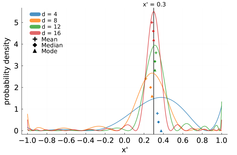
Figure 9: Distribution broadening due to the finite basis representation of a continuous value. Given a continuous value in the compact domain $x^{\prime}\in[-1,1]$, e.g., $x^{\prime}=0.3$, represented by the dotted black line, the corresponding conditional distribution under the finite Legendre basis representation is shown for varying $d$. Summary statistics (mean, median and mode) derived from each distribution are shown as colored markers.

For the purposes of imputation, however, the goal is to obtain a single representative estimate from the conditional distribution at a particular time point. To this end, we chose to investigate deterministic summary statistics derived from the conditional distribution, as opposed to individual random samples. We then defined an ‘encoding error’ $\epsilon_{d}$ to quantify the discrepancy introduced by the finite basis approximation:

$$\epsilon_{d}=\lvert x_{i}-\hat{x}_{i,d}\rvert\,,$$ (27)

where $x_{i}$ is a continuous value in the encoding domain, and $\hat{x}_{i,d}$ is a summary statistic derived from the conditional probability distribution at site $i$, after encoding $x_{i}$ as a discrete quantum state (via the encoding $\phi_{i}(x_{i})$) using a finite basis with dimension $d$. In Fig. 10, we compare the encoding error for three summary statistics – the expectation (mean), median, and mode – as a function of $d$ and the continuous value in the Legendre encoding domain $x_{i}\in[-1,1])$. As expected, the mean, shown in Fig. 10(a), exhibits large encoding errors across the domain, particularly for smaller $d$, as a result of its sensitivity to the artificial broadening of the distribution. The mode (Fig. 10(b)), while competitive for higher $d$, exhibits significant error spikes near the domain boundaries which can lead to erroneous imputations. The median, shown in Fig. 10(c), was found to consistently outperform other summary statistics, providing the lowest average error across the encoding domain. Motivated by these empirical findings, we chose to adopt the median, given that it best mitigates the effects of artificial broadening and ensures the most representative single point estimate from the encoded distribution.

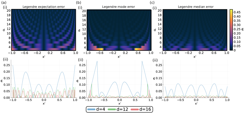
Figure 10: Encoding error over the Legendre domain. The absolute error between a known value $x^{\prime}$ in the encoding domain, and a summary statistic for the probability distribution corresponding to the conditional density matrix $\rho=\phi^{\dagger}(x^{\prime})\phi(x^{\prime})$ (note that the Legendre feature map $\phi$ is time independent), which we refer to as the encoding error $\epsilon_{d}$ (as in Eq. (27)) is shown for (a) the mean (expectation); (b) the mode; and, (c) the median. In subplot (i) of each main panel, the encoding error when using the summary statistic as the single point estimator, is shown for varying $d$ and $x^{\prime}$ across the compact Legendre encoding domain $x^{\prime}\in[-1,1]$. In each subplot (ii), we show the encoding error for a few selected values of $d$.

Appendix C Hyperparameter tuning for classification

For classification, the physical dimension $d$, maximum bond dimension $\chi_{\rm max}$ and learning rate $\eta$ were determined by hyperparameter tuning. The particular hyperparameter ranges we searched for each empirical dataset are summarized in the table below:

Hyperparameter	ECG	Power Demand	Astronomy
$d$	[2, 15]	[2, 4]	3
$\eta$	[0.001, 10.0]	[0.001, 10.0]	1.0
$\chi_{\rm max}$	[15, 50]	[15, 30]	30
encoding	Legendre	Legendre	Fourier

To carry out hyperparameter tuning for ECG and Power Demand, we used an off-the-shelf Julia implementation of the adaptive particle swarm optimization algorithm [66] with stratified 5-fold cross-validation. Since the Astronomy dataset was derived as a subset of the original KeplerLightCurves UCR dataset, no published results exist for the baseline methods. To ensure a fair comparison in this context, we evaluated the baseline methods using their default configurations, i.e., their out-of-box performance. While these default parameters are typically based on extensive hyperparameter studies, such investigations are not the focus of the present work. Instead, for our MPS-based classifier, we selected a parameter set that performed well in our preliminary experiments. It is important to note that this choice of parameters does not confer an unfair advantage: our 30-fold resampling strategy ensures that any given configuration performing well on one fold may not necessarily do so in others, as is the case for the default parameters of the baseline methods.

Appendix D Imputation algorithm details

Here we provide details on the specific steps of the imputation algorithm used in the main text. To elucidate the key steps of the proposed algorithm, consider a 6 site MPS trained on time-series instances of length $T=6$ samples from class C, shown in Fig. 11. Given an unseen time-series instance of data class C that is incomplete, for example, only the values $x_{2}$, $x_{4}$, $x_{6}$ are known, the goal of imputation is to estimate the unknown values (i.e., to ‘fill in the gaps’) - in this case, $x_{1}$, $x_{3}$, $x_{5}$. Our approach is performed in two main steps: (i) the trained MPS is conditioned on known values by first transforming them into quantum states and then projecting the MPS onto these known states; (ii) using the conditioned MPS, the unknown values are then determined by sequentially computing and sampling from a series of single-site reduced density matrices.

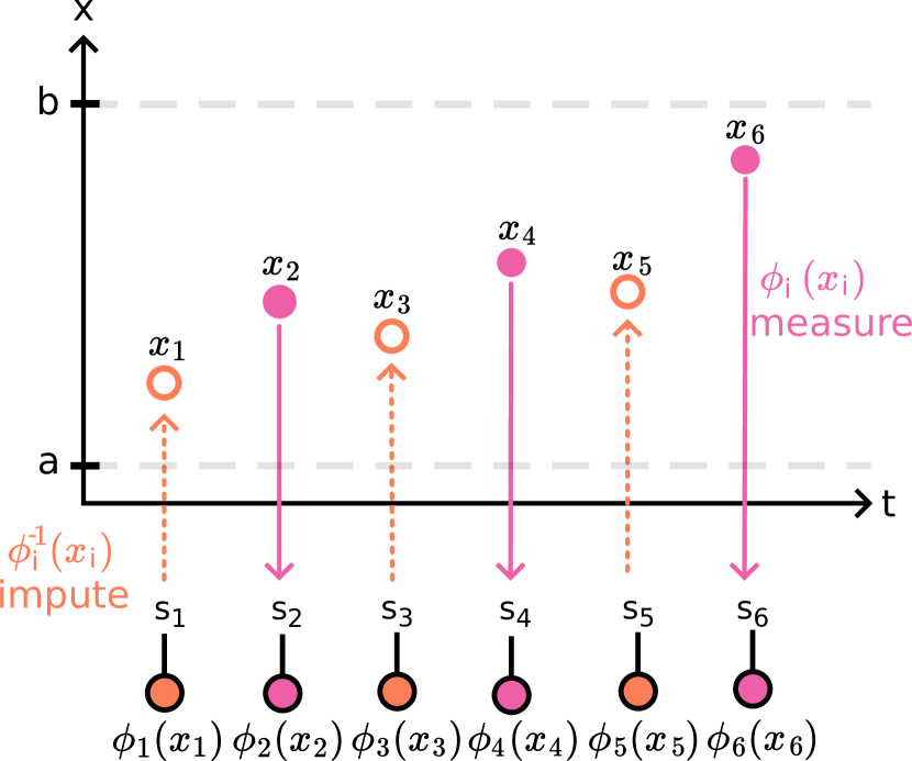
Figure 11: A toy imputation problem involving six time-series samples. Here, we consider three observed data points (solid pink markers) $x_{2}$, $x_{4}$, $x_{6}$, and three unobserved (missing) data points, $x_{1}$, $x_{3}$, $x_{5}$. Observed values in the encoding domain $x_{t}\in[a,b]$ are mapped to discrete quantum states (pink vectors) via the encoding $\phi_{i}(x_{i})$ i.e., $s_{i}=\phi_{i}(x_{i})$. The MPS is then conditioned on the observed values by making a series of projective measurements at the sites corresponding to the observed states, $s_{2}$, $s_{4}$, $s_{6}$. The unobserved states (orange vectors) are determined from the conditional probability distribution encoded by the partially conditioned MPS, and transformed back to time-series values in the encoding domain (orange markers) by an inverse transformation.

D.1 Projecting the trained MPS onto known states

The first step of the algorithm is to project the MPS - through a sequence of iterative site-wise measurements - into a subspace which can then be used to impute missing data. We assume the MPS $W$, which is trained to approximate the underlying joint PDF of class C time-series data, is L2 normalized. This normalization condition can be shown diagrammatically in Penrose graphical notation [49]) as:

where $s_{1},s_{2},\dots,s_{6}$ correspond to the physical indices at each site. Using the feature-mapped state associated with the first known value of the time series, $\phi_{2}(x_{2})$, a projective measurement is made at the corresponding MPS site $A_{2}$ by contracting its physical index with that of the state vector $\phi_{2}(x_{2})$ (shown in pink):

To ensure the updated MPS continues to represent a valid conditional probability distribution, the entries in the tensor corresponding to the measured site (dashed circle) are divided through by the factor $\sqrt{P(s_{2})}$, yielding a normalized MPS. To compute the marginal probability $P(s_{2})$, we perform a contraction operation with two copies of the MPS (one conjugated), first tracing over all remaining sites, and then contracting the state vector of interest $\phi_{2}(x_{2})$ with its corresponding MPS site (on both copies), shown diagrammatically as:

Note that in the main text, we refer to $P(x_{i})=P(\phi_{i}(x_{i}))$ in order to reduce notational clutter. The rescaled tensor is then contracted over the bond index with the adjacent site to yield an updated MPS that is one site shorter. Having projected the MPS onto the known state at the first site, the updated MPS now approximates the PDF conditioned on the known time-series value at $t=2$:

Here, we use open physical indices to represent the entire structure of the joint probability distribution over all possible configurations that $s_{1},s_{3},\dots,s_{6}$ can take. Using the known value of the time series at $t=4$ (pink vector), one then proceeds to make a second projective measurement of the MPS onto its corresponding state at the fourth site $A_{4}$ (now the third site), before normalizing the updated tensor by dividing through by $\sqrt{P(x_{4})}$ and contracting with its neighboring site:

Here, we show the resulting 4 site MPS which approximates the PDF conditional on having measured the states $s_{2},s_{4}$.

This process of making projective measurements, normalizing, and contracting with the neighboring site proceeds recursively for all remaining known data points, yielding a final MPS which approximates the PDF conditioned on all known time-series values:

with sites corresponding to the unknown states (time-series data points) that are to be imputed.

D.2 Imputing missing time-series data

The second step of the imputation algorithm involves determining the values of the unknown data points by estimating their respective values from the conditional PDF represented by the MPS. Here we use a sequential sampling approach which involves computing $d\times d$ single-site reduced density matrices.

We obtain the reduced density matrix $\rho_{1}$ of the first imputation site $A_{1}$ by tracing out the remaining sites $A_{3}$, $A_{6}$, shown diagrammatically as:

The probability density function (pdf) of the continuous variable $X$ is evaluated using the reduced density matrix $\rho$ as follows:

$$\textrm{pdf}_{X}(x)=\phi^{\dagger}(x)\rho\,\phi(x).$$ (28)

To sample a value for $x_{1}$ from the continuous distribution with this pdf, i.e., $x_{1}\sim\textrm{pdf}_{X}(x)$, one would typically resort to inverse transform sampling (see [21] and [20] for more details). However, for the purposes of imputation, our primary focus is on obtaining the best single-point estimate and its associated uncertainty, given the known data. This allows us to work directly with the reduced density matrix $\rho$, circumventing the need to generate individual samples. Using $\rho_{1}$, we calculate the median of the continuous random variable $X$, which serves as our best point estimate for $x_{1}$:

$$\text{median}(X)=\hat{x}\quad\text{such that}\quad\frac{1}{Z}\int_{-\infty}^{\hat{x}}f_{X}(x)\,dx=0.5,$$ (29)

where $\textrm{pdf}_{X}(x)$ is defined in Eq. 28 and $Z$ is a normalization factor:

$$Z=\int_{a}^{b}\textrm{pdf}_{X}(x)dx,$$ (30)

which ensures the pdf remains normalized over the support of the encoding domain $[a,b]$ ($[-1,1]$ for Legendre). For details about our choice of the median as the best single point estimate, see Appendix. B.

To quantify the uncertainty in our point estimate $\hat{x}$ we use the weighted median absolute deviation (WMAD):

$$\text{WMAD}(\hat{x})=\text{median}(\lvert x_{i}-\hat{x}\rvert,w_{i}),$$ (31)

where $\hat{x}$ is the median (our point estimate for $x_{1}$), $x_{i}$ are discretized values of the random variable $X$ within the encoding domain $[a,b]$, and the weights $w_{i}$ are proportional to the probability densities $w_{i}\propto\textrm{pdf}_{X}(x_{i})$.

Using the value of the point estimate $x_{1}$ and the associated state $\phi_{1}(x_{1})$, a projective measurement is made at the corresponding MPS site $A_{1}$, completing one step of the imputation algorithm. The process then continues recursively – at each step, obtaining the single site reduced density matrix $\rho_{1}$, computing the point estimate $x^{*}_{1}$, and performing a projective measurement – until all remaining unknown values have been determined:

To transform the imputed states (yellow vectors) back to their rescaled time-series values, one can apply the inverse of the feature map $\phi_{t}^{-1}(x)$. An additional transformation can be applied to convert the rescaled time-series (in the encoding domain) back to their respective amplitudes in the original data domain, i.e., .

Appendix E Inverse transform sampling

To generate single-shot time-series trajectories, as in Fig. 7, we used an inverse transform sampling (ITS) approach augmented with a rejection scheme to mitigate the effects of the encoding error discussed in Sec. B. Specifically, due to the finite basis approximation of (original continuous) time-series values, we observe an error which manifests as an artificial broadening of the conditional distribution of time-series values at each MPS site. As a consequence of this broadening, the conditional distribution can assign non-negligible probabilities to time-series values that would otherwise be highly improbable, as depicted in Fig. 9. When generating trajectories through conditional site-wise sampling – starting at the first site and proceeding sequentially to the end – these errors can propagate and compound, potentially leading to trajectories that are not representative of the underlying joint distribution. While increasing $d$, the number of basis functions in the encoding (as in Eq. (3)), can mitigate this error in principle, achieving meaningful reductions in distribution broadening would require values that render ITS computationally intractable for most applications. Instead, we use a rejection scheme to discard highly improbable values based on their deviation from the median (WMAD) of the conditional distribution. Our choice of the median was motivated empirically from the analysis presented in Appendix B.

To perform inverse transform sampling (ITS), given an MPS site $A_{i}$ corresponding to an unobserved time-series value $x_{i}$, we use the following procedure to sample the value from the corresponding conditional distribution, i.e., $x_{i}\sim pdf_{i}(x)$. First, we evaluate the cumulative distribution function, $F_{i}(x)$, as:

$$F_{i}(x)=\frac{1}{Z}\int_{a}^{x}\phi^{\dagger}(x^{\prime})\rho_{i}\phi_{i}(x^{\prime}){\mathrm{d}}x^{\prime}\,,$$ (32)

with $Z$ chosen so that $F_{s_{i}}(b)=1$, and where $a$ is the lower bound on the support of the encoding domain $[a,b]$. Next, we sample a random value from a uniform distribution defined on the interval $[0,1]$:

$$u\sim U(0,1).$$ (33)

Using the inverse cumulative distribution function, $F_{i}^{-1}(u)$, we select the value $x_{i}$ such that $F_{i}(x_{i})=u$. We then apply the WMAD-based rejection criteria described in Alg.1.

The selection of the rejection threshold factor $\alpha$ requires careful consideration. A threshold that is overly restrictive (i.e., small $\alpha$) would constrain the sampling space, potentially introducing bias by suppressing variability that is a feature of the true encoded distribution. Conversely, a less stringent threshold (i.e., large $\alpha$) would fail to adequately address the artificial broadening effects. Through empirical investigation, we identified $\alpha=2.0$ (i.e., $2\cdot\rm WMAD)$ as an effective heuristic, which provides a balance between the two extremes.

Algorithm 1 Single-shot time-series generation.

1:

2:Compute the conditional PDF, $\textrm{pdf}_{i}(x)$, at MPS site $A_{i}$.

3:Compute the conditional CDF as in Eq. (32).

4:Generate a uniform random number $u\sim U(0,1)$.

5:Find $x_{i}=F_{i}^{-1}(u)$ such that $F_{i}(x_{i})=u$.

6:Compute the median $m_{i}$ and WMAD $wm_{i}$ of the conditional distribution $pdf_{i}(x)$.

7:Evaluate the deviation of $x_{i}$ from $m_{i}$:

$$\Delta_{i}=|x_{i}-m_{i}|.$$

8:while $\Delta_{i}>\alpha\cdot wm_{i}$ do $\triangleright$ Rejection step

9:  Generate a new $u\sim U(0,1)$.

10:  Find $x_{i}=F_{i}^{-1}(u)$.

11:  Evaluate $\Delta_{i}$

12:end while

13:Accept $x_{i}$ as the $i$-th value in the trajectory.

Appendix F Real world time-series datasets

Here we provide further details on the three UCR time-series datasets used for the classification task in Sec.III.3, each representing key domain of application: (i) ECG (medicine), (ii) Power Demand (energy) and (iii) Astronomy (physics). Representative time-series examples from each dataset are shown in Fig. 12.

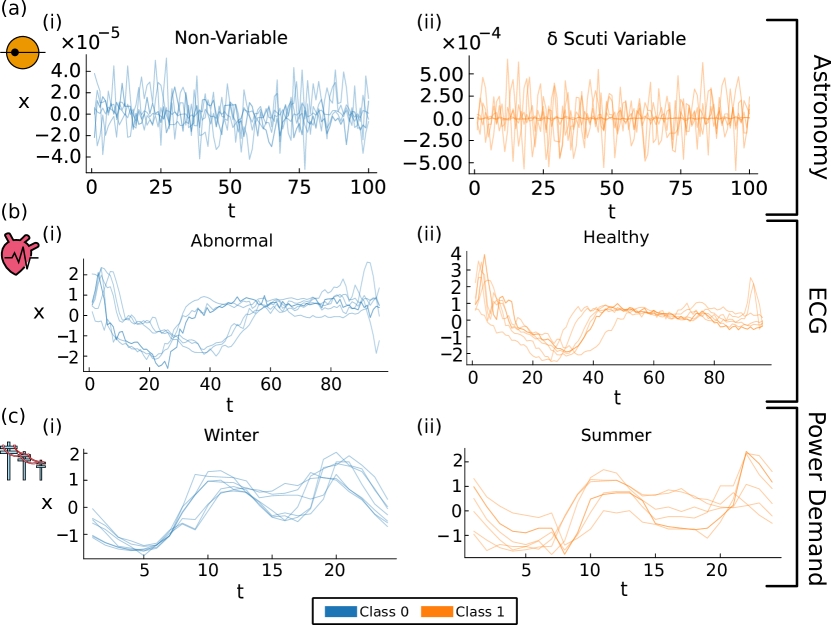
Figure 12: Representative time-series instances for each empirical dataset. Several time-series instances from each class are plotted on the same axis, and in the original data domain, for the three datasets: (a) Astronomy (2-class subset of KeplerLightCurves), (b) ECG (ECG200), and (c) Power Demand (ItalyPowerDemand). In each panel, we plot representative instances from (i) class 0, and (ii) class 1, for the various binary classification problems.

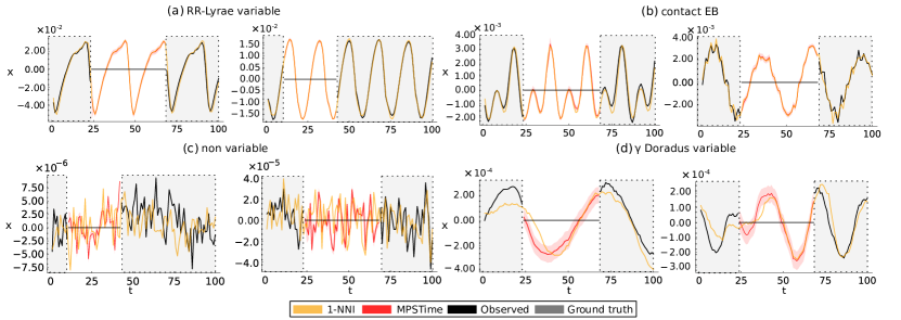
Figure 13: MPS imputations on unseen Astronomy time series with real data gaps caused by satellite transmission downlinks. The panels depict examples of MPS ($\chi_{\rm max}=35$, $d=12$) and 1-NNI on held-out instances with real data gaps from four classes of star system: (a) RR-Lyrae variable, (b) contact eclipsing binary (contact EB), (c) non variable, and (d) $\gamma$ Doradus variable. The flat horizontal lines in light gray correspond to real missing data which has been imputed with the time-series mean in the original UCR dataset.

F.1 Imputation on real-world data gaps

For our investigation of the Astronomy dataset in Sec. III.2 of the main text, we excluded time-series windows with true data gaps for which ground-truth values are unavailable. For completeness, to showcase how our method may perform with real missing data, we trained a $d=12$, $\chi_{\rm max}=35$ MPS on clean windows from four classes of star system: (i) RR-Lyrae variable; (ii) contact Eclipsing Binary (contact EB); (iii) non variable; and, (iv) Gamma Doradus variable ($\gamma$ Doradus variable). We then imputed real missing values on two held-out instances from each class and plotted a visual comparison with the 1-Nearest Neighbor Imputation (1-NNI) baseline in Fig. 13. Notably, while MPS and 1-NNI produce similar predictions for uniformly repetitive periodic light curves, such as RR-Lyrae and contact EB (Fig. 13a, b, respectively), they diverge for less uniform patterns, such as non variable and $\gamma$ Doradus variable (Fig. 13c, d, respectively).

Appendix G Time-series classification baselines

For classification performance baselines we selected three models, each representing a key category of time-series classifier; (i) distance-based, (ii) deep learning ensemble, (iii) hybrid:

• 1-NN-DTW: Nearest neighbor using a Dynamic Time Warping (DTW) similarity measure. Considered to be the most commonly used standard classical benchmark in much of the time-series classification literature [60].

• InceptionTime [61]: State-of-the-art deep learning classifier which consists of an ensemble of five Convolutional Neural Network (CNN) models.

• HC2 [62]: HC2 (HIVE-COTE V2.0) is an ensemble of classifiers, each built on different time-series data representations including phase-independent shapelets, bag-of-words based dictionaries, among others. HC2 is considered to be state-of-the-art for classification accuracy on the UCR repository.

For the Astronomy dataset, we used off-the-shelf implementations of the 1-NN-DTW, InceptionTime, and HC2 classifiers that are accessible at the Python aeon (v0.11.1) library [67]. For the InceptionTime baseline, we used the recommended hyperparameter values from the original implementation [61], which are set as defaults in aeon, and trained the model for 250 epochs on an NVIDIA L40S GPU. To facilitate a fair comparison, we allowed HC2 the same computational resources as InceptionTime by setting the build-time contract to match the maximum time taken to train InceptionTime on the same hardware. We also used default hyperparameters for HC2 provided in the aeon implementation.

Appendix H Time-series imputation baselines

In the main text, we compare our imputation algorithm with several state-of-the-art methods, each representing a unique architecture of time-series imputation model: (i) classical (1-NNI), (ii) diffusion model (CSDI), (iii) recurrent neural network (BRITS), and (iv) matrix completion method (CDRec):

• 1-NNI [46]: A special case of k-NNI (k-Nearest Neighbours Imputation), where $k=1$. 1-NNI substitutes missing data points in unseen time series with those from the Euclidean nearest neighbour time series in the training set.

• CSDI [56]: CSDI (Conditional Score-based Diffusion Imputation) is a generative approach to imputation which uses a neural network-based diffusion model to generate new data points that are consistent with the underlying data distribution.

• BRITS [57]: BRITS (Bidirectional recurrent imputation for time series) uses a recurrent neural network (RNN) architecture to handle missing values in time series.

• CDRec [55]: A matrix-based technique for memory efficient centroid decomposition (an approximation of SVD) of long time series.

For our benchmarking investigations, we used off-the-shelf implementations of the aforementioned algorithms which are readily available in the Python PyPOTS (v0.8) library [59]. Hyperparameters for each model were set to the default values provided with the implementation.

References

- Fannes et al. [1992] M. Fannes, B. Nachtergaele, and R. F. Werner, Communications in mathematical physics 144, 443 (1992).
- Cirac et al. [2021] J. I. Cirac, D. Pérez-García, N. Schuch, and F. Verstraete, Reviews of Modern Physics 93, 045003 (2021).
- Orús [2014] R. Orús, Annals of Physics 349, 117 (2014).
- Schollwoeck [2011] U. Schollwoeck, Annals of Physics 326, 96 (2011), arXiv:1008.3477 [cond-mat].
- Verstraete and Cirac [2006] F. Verstraete and J. I. Cirac, Physical Review B 73, 094423 (2006).
- Pirvu et al. [2012] B. Pirvu, G. Vidal, F. Verstraete, and L. Tagliacozzo, Phys. Rev. B 86, 075117 (2012).
- Manzoni et al. [2017] M. T. Manzoni, D. E. Chang, and J. S. Douglas, Nature Communications 8, 1743 (2017).
- Mahmoodian et al. [2020] S. Mahmoodian, G. Calajó, D. E. Chang, K. Hammerer, and A. S. Sørensen, Physical Review X 10, 031011 (2020).
- Pichler and Zoller [2016] H. Pichler and P. Zoller, Phys. Rev. Lett. 116, 093601 (2016).
- Mahmoodian [2019] S. Mahmoodian, Phys. Rev. Lett. 123, 133603 (2019).
- Vidal [2003] G. Vidal, Physical Review Letters 91, 147902 (2003).
- Tindall et al. [2024] J. Tindall, M. Fishman, E. M. Stoudenmire, and D. Sels, PRX Quantum 5, 010308 (2024).
- Oseledets [2011] I. V. Oseledets, SIAM Journal on Scientific Computing 33, 2295 (2011).
- Vidal [2004] G. Vidal, Physical Review Letters 93, 040502 (2004).
- Stoudenmire and Schwab [2017] E. M. Stoudenmire and D. J. Schwab, “Supervised Learning with Quantum-Inspired Tensor Networks,” (2017), arXiv:1605.05775 [cond-mat, stat].
- Han et al. [2018] Z.-Y. Han, J. Wang, H. Fan, L. Wang, and P. Zhang, Physical Review X 8, 031012 (2018).
- Dymarsky and Pavlenko [2022] A. Dymarsky and K. Pavlenko, Physical Review Research 4, 043111 (2022).
- Cheng et al. [2019] S. Cheng, L. Wang, T. Xiang, and P. Zhang, Physical Review B 99, 155131 (2019), arXiv:1901.02217 [cond-mat, physics:quant-ph, stat].
- Ran et al. [2020] S.-J. Ran, Z.-Z. Sun, S.-M. Fei, G. Su, and M. Lewenstein, Physical Review Research 2 (2020), 10.1103/PhysRevResearch.2.033293.
- Meiburg et al. [2023] A. Meiburg, J. Chen, J. Miller, R. Tihon, G. Rabusseau, and A. Perdomo-Ortiz, “Generative Learning of Continuous Data by Tensor Networks,” (2023), arXiv:2310.20498 [cond-mat, physics:quant-ph, stat].
- Mossi et al. [2024] A. Mossi, B. Žunkovic, and K. Flouris, “A Matrix Product State Model for Simultaneous Classification and Generation,” (2024), arXiv:2406.17441 [math-ph, physics:physics, physics:quant-ph, stat].
- Wang et al. [2020] J. Wang, C. Roberts, G. Vidal, and S. Leichenauer, “Anomaly Detection with Tensor Networks,” (2020), arXiv:2006.02516 [quant-ph, stat].
- Žunkovič [2023] B. Žunkovič, Neurocomputing 552, 126556 (2023), arXiv:2211.14085 [cs].
- Aizpurua et al. [2024] B. Aizpurua, S. Palmer, and R. Orus, “Tensor Networks for Explainable Machine Learning in Cybersecurity,” (2024), arXiv:2401.00867.
- Selvan and Dam [2020] R. Selvan and E. B. Dam, “Tensor Networks for Medical Image Classification,” (2020), arXiv:2004.10076 [cs, stat].
- Shi et al. [2022] X. Shi, Y. Shang, and C. Guo, Physical Review A 105, 052424 (2022), publisher: American Physical Society.
- Bai et al. [2022] S.-C. Bai, Y.-C. Tang, and S.-J. Ran, Chinese Physics Letters 39, 100701 (2022), arXiv:2207.06031 [cond-mat, physics:physics, physics:quant-ph].
- Liu et al. [2021] Y. Liu, W.-J. Li, X. Zhang, M. Lewenstein, G. Su, and S.-J. Ran, Frontiers in Applied Mathematics and Statistics 7 (2021).
- Bhatia et al. [2019] A. S. Bhatia, M. K. Saggi, A. Kumar, and S. Jain, “Matrix Product State Based Quantum Classifier,” (2019), arXiv:1905.01426 [quant-ph].
- Reyes and Stoudenmire [2020] J. Reyes and M. Stoudenmire, “A Multi-Scale Tensor Network Architecture for Classification and Regression,” (2020), arXiv:2001.08286 [quant-ph, stat].
- Araz and Spannowsky [2021] J. Y. Araz and M. Spannowsky, Journal of High Energy Physics 2021, 112 (2021), arXiv:2106.08334 [hep-ex, physics:hep-ph, physics:physics].
- Felser et al. [2021] T. Felser, M. Trenti, L. Sestini, A. Gianelle, D. Zuliani, D. Lucchesi, and S. Montangero, “Quantum-inspired Machine Learning on high-energy physics data,” (2021), arXiv:2004.13747 [cond-mat, physics:hep-ex, physics:physics, physics:quant-ph, stat].
- Guidotti et al. [2018] R. Guidotti, A. Monreale, S. Ruggieri, F. Turini, D. Pedreschi, and F. Giannotti, “A Survey Of Methods For Explaining Black Box Models,” (2018), arXiv:1802.01933 [cs].
- Fulcher [2018] B. D. Fulcher, in Feature Engineering for Machine Learning and Data Analytics, edited by Guozhu Dong and Huan Liu (CRC Press, Boca Raton, 2018) 1st ed., pp. 87–116.
- Lu et al. [2021] S. Lu, M. Kan’asz-Nagy, I. Kukuljan, and J. I. Cirac, ArXiv abs/2103.06872 (2021).
- Fulcher et al. [2013] B. D. Fulcher, M. A. Little, and N. S. Jones, Journal of The Royal Society Interface 10, 20130048 (2013), publisher: Royal Society.
- Kullback and Leibler [1951] S. Kullback and R. A. Leibler, The Annals of Mathematical Statistics 22, 79 (1951), publisher: Institute of Mathematical Statistics.
- Li and Zhang [2018] Z. Li and P. Zhang, “Shortcut Matrix Product States and its applications,” (2018), arXiv:1812.05248 [cond-mat, physics:quant-ph, stat].
- Sun et al. [2020a] Z.-z. Sun, S.-j. Ran, and G. Su, Physical Review E 102, 012152 (2020a), arXiv:2001.04029 [cond-mat, stat].
- Liu et al. [2023a] J. Liu, S. Li, J. Zhang, and P. Zhang, Physical Review E 107, L012103 (2023a), arXiv:2106.12974 [cond-mat, physics:quant-ph, stat].
- Kreutz-Delgado [2009] K. Kreutz-Delgado, arXiv preprint arXiv:0906.4835 (2009).
- Wang et al. [2024] J. Wang, W. Du, W. Cao, K. Zhang, W. Wang, Y. Liang, and Q. Wen, “Deep Learning for Multivariate Time Series Imputation: A Survey,” (2024), arXiv:2402.04059 [cs].
- Fang and Wang [2020] C. Fang and C. Wang, “Time Series Data Imputation: A Survey on Deep Learning Approaches,” (2020), arXiv:2011.11347.
- Garcıa et al. [2014] R. A. Garcıa, S. Mathur, S. Pires, C. Regulo, B. Bellamy, P. L. Palle, J. Ballot, S. B. Forteza, P. G. Beck, T. R. Bedding, T. Ceillier, T. R. Cortes, D. Salabert, and D. Stello, “Impact on asteroseismic analyses of regular gaps in Kepler data,” (2014), arXiv:1405.5374.
- Osman et al. [2018] M. S. Osman, A. M. Abu-Mahfouz, and P. R. Page, IEEE Access 6, 63279 (2018), conference Name: IEEE Access.
- Beretta and Santaniello [2016] L. Beretta and A. Santaniello, BMC Medical Informatics and Decision Making 16, 74 (2016).
- Luo et al. [2018] Y. Luo, X. Cai, Y. ZHANG, J. Xu, and Y. xiaojie, in Advances in Neural Information Processing Systems, Vol. 31 (Curran Associates, Inc., 2018).
- McCoy et al. [2018] J. T. McCoy, S. Kroon, and L. Auret, IFAC-PapersOnLine 5th IFAC Workshop on Mining, Mineral and Metal Processing MMM 2018, 51, 141 (2018).
- Penrose et al. [1971] R. Penrose et al., Combinatorial mathematics and its applications 1, 221 (1971).
- Ferris and Vidal [2012] A. J. Ferris and G. Vidal, Physical Review B 85, 165146 (2012), arXiv:1201.3974 [cond-mat, physics:quant-ph].
- Olszewski et al. [2001] R. T. Olszewski, R. A. Maxion, and D. P. Siewiorek (2001).
- Dau et al. [2019] H. A. Dau, A. Bagnall, K. Kamgar, C.-C. M. Yeh, Y. Zhu, S. Gharghabi, C. A. Ratanamahatana, and E. Keogh, “The UCR Time Series Archive,” (2019), arXiv:1810.07758.
- Keogh et al. [2006] E. Keogh, L. Wei, X. Xi, S. Lonardi, J. Shieh, and S. Sirowy, in Sixth International Conference on Data Mining (ICDM’06) (IEEE, Hong Kong, China, 2006) pp. 912–916, iSSN: 1550-4786.
- Barbara et al. [2022] N. H. Barbara, T. R. Bedding, B. D. Fulcher, S. J. Murphy, and T. Van Reeth, Monthly Notices of the Royal Astronomical Society 514, 2793 (2022).
- Khayati et al. [2014] M. Khayati, M. Bohlen, and J. Gamper, in 2014 IEEE 30th International Conference on Data Engineering (IEEE, Chicago, IL, USA, 2014) pp. 100–111.
- Tashiro et al. [2021] Y. Tashiro, J. Song, Y. Song, and S. Ermon, “CSDI: Conditional Score-based Diffusion Models for Probabilistic Time Series Imputation,” (2021), arXiv:2107.03502.
- Cao et al. [2018] W. Cao, D. Wang, J. Li, H. Zhou, L. Li, and Y. Li, in Neural Information Processing Systems (2018).
- Khayati et al. [2020] M. Khayati, A. Lerner, Z. Tymchenko, and P. Cudré-Mauroux, Proceedings of the VLDB Endowment 13, 768 (2020).
- Du [2023] W. Du, arXiv preprint arXiv:2305.18811 (2023).
- Bagnall et al. [2017] A. Bagnall, J. Lines, A. Bostrom, J. Large, and E. Keogh, Data Mining and Knowledge Discovery 31, 606 (2017).
- Fawaz et al. [2020] H. I. Fawaz, B. Lucas, G. Forestier, C. Pelletier, D. F. Schmidt, J. Weber, G. I. Webb, L. Idoumghar, P.-A. Muller, and F. Petitjean, Data Mining and Knowledge Discovery 34, 1936 (2020), arXiv:1909.04939 [cs, stat].
- Middlehurst et al. [2021] M. Middlehurst, J. Large, M. Flynn, J. Lines, A. Bostrom, and A. Bagnall, “HIVE-COTE 2.0: a new meta ensemble for time series classification,” (2021), arXiv:2104.07551 [cs].
- Middlehurst et al. [2024a] M. Middlehurst, P. Schäfer, and A. Bagnall, Data Mining and Knowledge Discovery 38, 1958 (2024a).
- Ismail-Fawaz et al. [2022] A. Ismail-Fawaz, M. Devanne, J. Weber, and G. Forestier, in 2022 IEEE International Conference on Big Data (Big Data) (2022) pp. 972–981.
- Hayashi et al. [2015] M. Hayashi, S. Ishizaka, A. Kawachi, G. Kimura, and T. Ogawa, in Introduction to Quantum Information Science, edited by M. Hayashi, S. Ishizaka, A. Kawachi, G. Kimura, and T. Ogawa (Springer, Berlin, Heidelberg, 2015) pp. 127–166.
- Zhan et al. [2009] Z.-H. Zhan, J. Zhang, Y. Li, and H. S.-H. Chung, IEEE Transactions on Systems, Man, and Cybernetics, Part B (Cybernetics) 39, 1362 (2009), conference Name: IEEE Transactions on Systems, Man, and Cybernetics, Part B (Cybernetics).
- Middlehurst et al. [2024b] M. Middlehurst, A. Ismail-Fawaz, A. Guillaume, C. Holder, D. G. Rubio, G. Bulatova, L. Tsaprounis, L. Mentel, M. Walter, P. Schäfer, and A. Bagnall, “aeon: a Python toolkit for learning from time series,” (2024b), arXiv:2406.14231.
- Bai and Ran [2024] S.-C. Bai and S.-J. Ran, “Universal replication of chaotic characteristics by classical and quantum machine learning,” (2024), arXiv:2405.08484.
- Rubin [1975] D. B. Rubin, ETS Research Bulletin Series 1975, i (1975), _eprint: https://onlinelibrary.wiley.com/doi/pdf/10.1002/j.2333-8504.1975.tb01053.x.
- Xu et al. [2023] M. A. Xu, A. Moreno, S. Nagesh, V. B. Aydemir, D. W. Wetter, S. Kumar, and J. M. Rehg, “PulseImpute: A Novel Benchmark Task for Pulsative Physiological Signal Imputation,” (2023), arXiv:2212.07514 [cs].
- Du et al. [2024] W. Du, J. Wang, L. Qian, Y. Yang, F. Liu, Z. Wang, Z. Ibrahim, H. Liu, Z. Zhao, Y. Zhou, W. Wang, K. Ding, Y. Liang, B. A. Prakash, and Q. Wen, “TSI-Bench: Benchmarking Time Series Imputation,” (2024), arXiv:2406.12747 [cs].
- Ismail et al. [2022] A. R. Ismail, N. Z. Abidin, and M. K. Maen, Journal of Robotics and Control (JRC) 3, 143 (2022).
- Phan [2020] T.-T.-H. Phan, in 2020 International Conference on Multimedia Analysis and Pattern Recognition (MAPR) (2020) pp. 1–6.
- Zhang and Qi [2005] G. Zhang and M. Qi, European Journal of Operational Research 160, 501 (2005).
- Weerakody et al. [2021] P. B. Weerakody, K. W. Wong, G. Wang, and W. Ela, Neurocomputing 441, 161 (2021).
- Li et al. [2009] L. Li, J. McCann, N. S. Pollard, and C. Faloutsos, in Proceedings of the 15th ACM SIGKDD international conference on Knowledge discovery and data mining (ACM, Paris France, 2009) pp. 507–516.
- Zhang [2012] S. Zhang, Journal of Systems and Software 85, 2541 (2012).
- Khayati et al. [2015] M. Khayati, M. H. Böhlen, and P. C. Mauroux, in Advances in Spatial and Temporal Databases, Vol. 9239, edited by C. Claramunt, M. Schneider, R. C.-W. Wong, L. Xiong, W.-K. Loh, C. Shahabi, and K.-J. Li (Springer International Publishing, Cham, 2015) pp. 237–254, series Title: Lecture Notes in Computer Science.
- Yoon et al. [2019] J. Yoon, W. R. Zame, and M. van der Schaar, IEEE Transactions on Biomedical Engineering 66, 1477 (2019), conference Name: IEEE Transactions on Biomedical Engineering.
- Liu et al. [2023b] M. Liu, H. Huang, H. Feng, L. Sun, B. Du, and Y. Fu, in 2023 IEEE 39th International Conference on Data Engineering (ICDE) (2023) pp. 1927–1939, iSSN: 2375-026X.
- Yang et al. [2024] L. Yang, Z. Zhang, Y. Song, S. Hong, R. Xu, Y. Zhao, W. Zhang, B. Cui, and M.-H. Yang, “Diffusion Models: A Comprehensive Survey of Methods and Applications,” (2024), arXiv:2209.00796 [cs].
- Kazijevs and Samad [2023] M. Kazijevs and M. D. Samad, Journal of Biomedical Informatics 144, 104440 (2023).
- Yang et al. [2020] F. Yang, J. Du, J. Lang, W. Lu, L. Liu, C. Jin, and Q. Kang, BioMed Research International 2020, 7141725 (2020), _eprint: https://onlinelibrary.wiley.com/doi/pdf/10.1155/2020/7141725.
- Ran and Su [2023] S.-J. Ran and G. Su, Intelligent Computing 2, 0061 (2023), publisher: American Association for the Advancement of Science.
- Kobayashi et al. [2024] N. Kobayashi, Y. Suimon, and K. Miyamoto, “Time series generation for option pricing on quantum computers using tensor network,” (2024), arXiv:2402.17148 [quant-ph, q-fin].
- Bates et al. [2004] S. Bates, J. Sienz, and V. Toropov, in 45th AIAA/ASME/ASCE/AHS/ASC Structures, Structural Dynamics & Materials Conference, Structures, Structural Dynamics, and Materials and Co-located Conferences (American Institute of Aeronautics and Astronautics, 2004).
- Selvan et al. [2022] R. Selvan, E. B. Dam, S. A. Flensborg, and J. Petersen, “Patch-based Medical Image Segmentation using Matrix Product State Tensor Networks,” (2022), arXiv:2109.07138 [cs].
- Zhao et al. [2016] Q. Zhao, G. Zhou, S. Xie, L. Zhang, and A. Cichocki, “Tensor Ring Decomposition,” (2016), arXiv:1606.05535 [cs].
- Wall and D’Aguanno [2021] M. L. Wall and G. D’Aguanno, Physical Review A 104, 042408 (2021).
- Rieser et al. [2023] H.-M. Rieser, F. Köster, and A. P. Raulf, Proceedings of the Royal Society A: Mathematical, Physical and Engineering Sciences 479, 20230218 (2023), publisher: Royal Society.
- Wright et al. [2022] L. Wright, F. Barratt, J. Dborin, V. Wimalaweera, B. Coyle, and A. G. Green, “Deterministic Tensor Network Classifiers,” (2022), arXiv:2205.09768 [cond-mat, physics:quant-ph].
- Weyrauch and Rakov [2013] M. Weyrauch and M. V. Rakov, Ukrainian Journal of Physics 58, 657 (2013), arXiv:1303.1333 [cond-mat].
- Pippan et al. [2010] P. Pippan, S. R. White, and H. G. Evertz, Physical Review B 81, 081103 (2010), publisher: American Physical Society.
- Lin et al. [2023] S.-H. Lin, O. Kuijpers, S. Peterhansl, and F. Pollmann, “Distributive Pre-Training of Generative Modeling Using Matrix-Product States,” (2023), arXiv:2306.14787 [cond-mat, physics:quant-ph].
- Lubba et al. [2019] C. H. Lubba, S. S. Sethi, P. Knaute, S. R. Schultz, B. D. Fulcher, and N. S. Jones, Data Mining and Knowledge Discovery 33, 1821 (2019).
- Hauru et al. [2021] M. Hauru, M. Van Damme, and J. Haegeman, SciPost Physics 10, 040 (2021), arXiv:2007.03638 [cond-mat, physics:quant-ph].
- Lin et al. [2021] H. Lin, S. Ye, and X. Zhu, “Tensor Network for Supervised Learning at Finite Temperature,” (2021), arXiv:2104.05439 [cs].
- Strashko and Stoudenmire [2022] A. Strashko and E. M. Stoudenmire, “Generalization and Overfitting in Matrix Product State Machine Learning Architectures,” (2022), arXiv:2208.04372 [quant-ph].
- Meng et al. [2023] Y.-M. Meng, J. Zhang, P. Zhang, C. Gao, and S.-J. Ran, SciPost Physics 14, 142 (2023).
- Sun et al. [2020b] Z.-Z. Sun, C. Peng, D. Liu, S.-J. Ran, and G. Su, Physical Review B 101, 075135 (2020b).
- Bagnall et al. [2016] A. Bagnall, A. Bostrom, J. Large, and J. Lines, “The Great Time Series Classification Bake Off: An Experimental Evaluation of Recently Proposed Algorithms. Extended Version,” (2016), arXiv:1602.01711 [cs].
- Weigold et al. [2021] M. Weigold, J. Barzen, F. Leymann, and M. Salm, IET Quantum Communication 2, 141 (2021), _eprint: https://onlinelibrary.wiley.com/doi/pdf/10.1049/qtc2.12032.
- Wall et al. [2021] M. L. Wall, M. R. Abernathy, and G. Quiroz, Physical Review Research 3, 023010 (2021).
- Sengupta et al. [2022] R. Sengupta, S. Adhikary, I. Oseledets, and J. Biamonte, “Tensor networks in machine learning,” (2022), arXiv:2207.02851 [cond-mat, physics:quant-ph].
- Schuld and Killoran [2019] M. Schuld and N. Killoran, Physical Review Letters 122, 040504 (2019), arXiv:1803.07128 [quant-ph].
- Psarras et al. [2022] C. Psarras, L. Karlsson, J. Li, and P. Bientinesi, “The landscape of software for tensor computations,” (2022), arXiv:2103.13756 [cs].
- Pérez-Salinas et al. [2020] A. Pérez-Salinas, A. Cervera-Lierta, E. Gil-Fuster, and J. I. Latorre, Quantum 4, 226 (2020), arXiv:1907.02085 [quant-ph].
- Novikov et al. [2017] A. Novikov, M. Trofimov, and I. Oseledets, “Exponential Machines,” (2017), arXiv:1605.03795 [cs, stat].
- Martyn et al. [2020] J. Martyn, G. Vidal, C. Roberts, and S. Leichenauer, “Entanglement and Tensor Networks for Supervised Image Classification,” (2020), arXiv:2007.06082 [quant-ph, stat].
- Lloyd et al. [2020] S. Lloyd, M. Schuld, A. Ijaz, J. Izaac, and N. Killoran, “Quantum embeddings for machine learning,” (2020), arXiv:2001.03622 [quant-ph].
- Liu et al. [2019] D. Liu, S.-J. Ran, P. Wittek, C. Peng, R. B. García, G. Su, and M. Lewenstein, New Journal of Physics 21, 073059 (2019).
- Huggins et al. [2019] W. Huggins, P. Patel, K. B. Whaley, and E. M. Stoudenmire, Quantum Science and Technology 4, 024001 (2019), arXiv:1803.11537 [cond-mat, physics:quant-ph].
- LaRose and Coyle [2020] R. LaRose and B. Coyle, Physical Review A 102, 032420 (2020), arXiv:2003.01695 [quant-ph].
- Guo et al. [2018] C. Guo, Z. Jie, W. Lu, and D. Poletti, Physical Review E 98, 042114 (2018), arXiv:1803.10908 [cond-mat, physics:nlin].
- Dilip et al. [2022] R. Dilip, Y.-J. Liu, A. Smith, and F. Pollmann, Physical Review Research 4, 043007 (2022), publisher: American Physical Society.
- Dborin et al. [2022] J. Dborin, F. Barratt, V. Wimalaweera, L. Wright, and A. G. Green, Quantum Science and Technology 7, 035014 (2022), publisher: IOP Publishing.