3D non-linear non-adiabatic MHD simulations of core density collapse event in LHD plasma

Abstract

A new three-dimensional, non-linear, non-adiabatic Magnetohydrodynamics (MHD) model has been implemented in MIPS code, which takes into account the parallel heat diffusivity. The model has been benchmarked against the former MHD model used in MIPS code. A preliminary study of the core density collapse event (CDC) observed in the Large Helical Device (LHD) plasma has been performed using the new model. The equilibrium has been constructed using HINT code for axis $\beta=4\%$ plasma with a steep pressure gradient, which makes the plasma potentially unstable in the LHD. The model can show preliminary characteristics of the CDC event. The work is extended to analyze the effect of an external heating source on the CDC event. An external heat source centered at the core of the plasma triggers the CDC event earlier than the time of spontaneous CDC, caused by the increase in pressure gradient steepness. The amplitude and geometry of the heat source have been observed to have an effect on the MHD stability.

• December 2024

Keywords: 3D non-linear MHD simulations, non-adiabatic, core density collapse event, stellarator, heat source

1 Introduction

In the LHD experiment, high-pressure configurations with internal diffusion barrier (IDB) have been achieved [1], which allow higher beta ($\beta$) values and improved confinement of the plasma. Increasing $\beta$ causes the rotational transform to become flatter or even reversed [2]. The high $\beta$ configuration with large Shafranov shift and IDB is prone to being unstable under the core density collapse (CDC) event [3] due to the steep pressure gradient interaction with the bad curvature region. In the regions where there is bad curvature, ballooning mode instabilities are expected to appear, which are one of the candidates for the triggering mechanism of the CDC event [4, 2, 5]. The CDC event drops the density profile in the core region, while keeping the temperature profile, on a fast timescale, affecting the fusion performance of the device.

In this work, a new $3$D non-linear non-adiabatic MHD model has been developed in MIPS code [6] including parallel heat diffusivity. The developed MHD equations represent the time evolution of plasma density $(n)$, momentum $(\rho\mathbf{v})$ and single fluid temperature $(T=T_{\rm i}+T_{\rm e})$. The approach allows us to analyze the density and the temperature dynamics, including anisotropic plasma heat diffusivity, and particle and heat sources. In this study, the improvement of the developed model compared to the former model of the code is the inclusion of external particle and heat sources, which serves to consider the fueling and heating system, such as Electron cyclotron heating (ECH) or Ion cyclotron resonance heating (ICRH). In order to analyze the process of CDC, a 3D MHD equilibrium with a steep pressure profile in the core region has been prepared using the HINT code [7, 8]. The equilibrium profile mimics the plasma with an internal diffusion barrier (IDB), which is considered to cause the CDC event. The non-linear MHD evolution is computed using the MIPS code based on the equilibrium produced by HINT. Furthermore, the effect of external heating on plasma response has been analyzed.

The manuscript is organized as follows. In Section 2 the new set of equations and the benchmark of the developed model are discussed. In Section 3 the analysis of the CDC event and the effects of external heating are discussed. Conclusions and perspectives are summarized in Section 4.

2 Model equations and methodology

A new 3D non-linear non-adiabatic MHD model has been implemented in MIPS code [6]. The developed model solves the evolution of the density $n$, momentum $\rho\mathbf{v}$, single-fluid temperature $T=T_{e}+T_{i}$, magnetic field $\mathbf{B}$, electric field $\mathbf{E}$ and current density $\mathbf{J}$:

$$\frac{\partial n}{\partial t}= -\nabla\cdot(n\mathbf{v})+\nabla\cdot(D_{\perp}\nabla(n-n_{\rm eq}))+S_{\rm n},$$ (1)

$$\eqalign{\frac{\partial\rho\mathbf{v}}{\partial t}=&-\nabla\cdot(\rho\mathbf{v}\mathbf{v})-\nabla(nT)+\mathbf{J}\times\mathbf{B}\\ &+\nabla\cdot\bigg{(}\rho\nu\bigg{[}\nabla\mathbf{v}+(\nabla\mathbf{v})^{\rm T}-\frac{2}{3}(\nabla\cdot\mathbf{v})\mathbb{I}\bigg{]}\bigg{)},}$$ (4)

$$\eqalign{\frac{\partial T}{\partial t}=&-\nabla\cdot(T\mathbf{v})-(\gamma-2)T\nabla\cdot\mathbf{v}\\ &+\frac{1}{n}\bigg{[}\nabla\cdot\bigg{(}n\chi_{\perp}\bigg{(}\nabla_{\perp}T-\nabla_{\perp,\rm eq}T_{\rm eq}\bigg{)}\bigg{)}\bigg{]}\\ &+\frac{1}{n}\bigg{[}\nabla\cdot\bigg{(}n\chi_{\parallel}\bigg{(}\nabla_{\parallel}T-\nabla_{\parallel,\rm eq}T_{\rm eq}\bigg{)}\bigg{)}\bigg{]}\\ &-\frac{T}{n}\bigg{[}\nabla\cdot(D_{\perp}\nabla(n-n_{\rm eq}))+S_{\rm n}\bigg{]}\\ &+S_{\rm T},}$$ (10)

$$\mathbf{E}=-\mathbf{v}\times\mathbf{B}+\eta(\mathbf{J}-\mathbf{J}_{\rm eq}),$$ (11)

$$\partial_{t}\mathbf{B}=\nabla\times\mathbf{E},$$ (12)

$$\nabla\times\mathbf{B}=\mu_{\rm 0}\mathbf{J},$$ (13)

where $\rho$ is the mass density, viscosity is $\nu$, and resistivity $\eta$. Particle and heat diffusivities are $D_{\perp}$ and $\chi$. Heat diffusivity is split into parallel ($\parallel$) and perpendicular ($\perp$) components to account for the anisotropic effects of thermal diffusion. The subscript “eq” is the equilibrium component, $\gamma=5/3$ is the adiabatic constant and $\mu_{0}$ is the vacuum permeability. $S_{\rm n}$ and $S_{\rm T}$ are the particle and heat sources, respectively. $S_{\rm T}$ includes a correction term for the particle source, i.e. $S_{\rm T}=(\gamma-1)(\hat{S}_{\rm T}+(1/2)v^{2}S_{\rm n}/n)$, where $\hat{S}_{\rm T}$ is an external heat source. The parallel and perpendicular gradients are defined as $\nabla_{\parallel}=\mathbf{b}(\mathbf{b}\cdot\nabla)$,$\nabla_{\parallel,\rm eq}=(\mathbf{b}-\mathbf{b}_{\rm eq})(\mathbf{b}_{\rm eq}\cdot\nabla)$ and $\nabla_{\perp}=\nabla-\nabla_{\parallel}$. The numerical grid is an equispaced, rectangular cylindrical coordinate grid $(R,\phi,Z)$. Time integration is computed using the 4th-order explicit Runge-Kutta scheme. The spatial derivatives are computed using the $4$th-order central difference method in each dimension. Periodic boundary conditions are used for the toroidal direction. A binary mask is used to solve the evolution of $n$, $\rho\mathbf{v}$, $T$, $\mathbf{B}$, $\mathbf{E}$ and $\mathbf{J}$ inside of the mask, and $\mathbf{B}$, $\mathbf{E}$ and $\mathbf{J}$ outside of it. In this work, the binary mask boundary is set at the last closed flux surface (LCFS). The code uses MPI parallelization (see [9] for scaling of parallel computing performance).

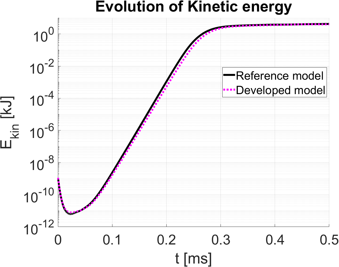
Figure 1: Kinetic energy evolution of LHD $\beta_{\rm axis}=4\%$ plasma for benchmark of the developed model (dotted pink) against the reference model (solid black).

The developed model has been benchmarked against the former MHD model in MIPS code. Time evolution of the kinetic energies of these two MHD models is shown in Figure 1. It has been verified that, using the same plasma parameters, the developed model can reproduce the same evolution of kinetic energy as well as the energy growth rate as the former model.

3 Simulation results

The 3D MHD equilibrium is calculated by HINT code. HINT code allows changes in the magnetic topology due to the non-linear 3D equilibrium response, which is the lowest order plasma response appearing in the 3D steady state [7, 8]. The properties of the constructed equilibrium are discussed in Section 3.1. The 3D non-linear MHD evolution is calculated by MIPS code, based on the 3D equilibrium, which is prepared by HINT code. The analysis of the spontaneous CDC event, $i.e.$ the instability intrinsic to the configuration without any external source, is discussed in Section 3.2. The work is extended to include the effect of external heat sources. The study of the effect of external heating source on the plasma response is discussed in Section 3.3.

3.1 3D equilibrium of LHD plasma

The 3D full-torus MHD equilibrium is constructed using HINT code, which considers the stochastic regions of the magnetic field and the existence of magnetic islands. The modeled 3D equilibrium is the LHD plasma configuration of axis $\beta=4\%$, which is particularly unstable and undergoes the CDC event. The equilibrium is obtained parting from the vacuum magnetic configuration and a parabolic initial guess given to the pressure profile. Then the plasma profile and the magnetic configuration are evolved until convergence, which satisfies the MHD equilibrium, is reached. It assumes a static equilibrium, $i.e.$, $\mathbf{v}=\mathbf{0}$. The density profile is approximated by a polynomial function of the normalized toroidal flux as:

$$n\propto n_{\rm axis}(1-\Phi_{\rm N})(1-\Phi_{\rm N}^{4}),$$ (14)

where $n_{\rm axis}$ is the axis density amplitude and $\Phi_{\rm N}$ is the normalized toroidal flux. The equilibrium temperature profile is determined by $P=nT=n(T_{\rm i}+T_{\rm e})$. Figure 2 shows the equilibrium plasma profile versus major radius of: pressure, density, temperature and normalized toroidal flux, that are obtained by HINT code process.

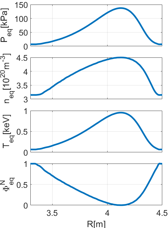
Figure 2: Plasma profiles versus major radius at $Z=$0\text{\,}\,\mathrm{m}$$ and $\phi=(1/2)(2\pi/10)$ of the equilibrium pressure (top), density ($2$nd), temperature ($3$rd), and normalized toroidal flux (bottom).

The central density is $n_{\rm axis}=$4.5\text{\times}{10}^{20}\text{\,}\,\mathrm{m}^{-3}$$, and the edge value is $n_{\rm edge}=$3.15\text{\times}{10}^{20}\text{\,}\,\mathrm{m}^{-3}$$. The temperature at the axis is $T_{0}=$0.95\text{\,}\,\mathrm{k}\mathrm{e}\mathrm{V}$$, and at the edge is $T_{\rm edge}=$0.07\text{\,}\,\mathrm{k}\mathrm{e}\mathrm{V}$$. The pressure at the axis is $P_{\rm axis}=$137.3\text{\,}\,\mathrm{k}\mathrm{P}\mathrm{a}$$ and at the edge $P_{\rm edge}=$6.85\text{\,}\,\mathrm{k}\mathrm{P}\mathrm{a}$$. This equilibrium profile mimics the plasma configuration with an internal diffusion barrier (IDB), which causes the CDC event. The LHD device has a periodicity of $10$, meaning that each periodic region spans $2\pi/10$ radians. The toroidal angle $\phi=0$ corresponds to the vertically elongated poloidal slice, while $\phi=(1/2)(2\pi/10)$ corresponds to the horizontally elongated poloidal slice. In the horizontally elongated poloidal slice, Thomson scattering diagnostics are utilized to measure electron temperature and density along the major radius [10]. For this, the latter poloidal slice is chosen as the angle to be analyzed in this study.

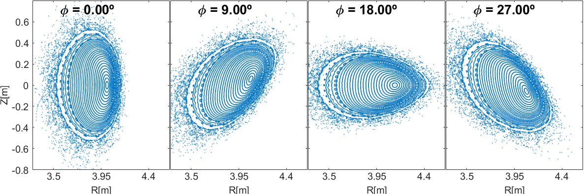
Figure 3: Poincaré plot of four different equispaced poloidal slices in the first periodic region $\phi=[0,2\pi/10]$ of the 3D equilibrium constructed using HINT.

Figure 3 shows the Poincaré plot of the 3D equilibrium together with the plasma shape variation along the toroidal angle for $4$ different slices, covering an entire periodic region $\phi=[0,2\pi/10]$. Clear magnetic flux surfaces are observed in the core region. Strong Shafranov shift is observed due to the high beta value. The edge region shows stochastic characteristics.

3.2 Spontaneous CDC event and its characteristics

The 3D non-linear MHD evolution is computed using MIPS code based on the 3D equilibrium discussed in the previous section. The major radius of LHD is $R_{\rm axis}=$3.6\text{\,}\,\mathrm{m}$$. The considered magnetic field and density at the axis are $B_{\rm axis}=$3\text{\,}\,\mathrm{T}$$ and $n_{\rm axis}=$4.5\text{\times}{10}^{20}\text{\,}\,\mathrm{m}^{-3}$$, respectively. The spatial grid resolution is $(R,\phi,Z)=(128,640,128)$. Particle and perpendicular heat diffusivity are uniform over the simulation domain, with values $D_{\perp}=$1.1\text{\,}\,\mathrm{m}^{2}\mathrm{s}^{-1}$$ and $\chi_{\perp}=$1.1\text{\times}{10}^{2}\text{\,}\,\mathrm{m}^{2}\mathrm{s}^{-1}$$, respectively. Viscosity, resistivity and parallel heat diffusivity are temperature dependent, i.e. $\nu(T)\propto\nu_{\rm axis}(T/T_{0})^{-3/2}$, $\eta(T)\propto\eta_{\rm axis}(T/T_{0})^{-3/2}$ and $\chi_{\parallel}(T,n)\propto\chi_{\parallel,\rm axis}(T/T_{0})^{5/2}/n$, where the values at the axis are: $\nu_{\rm axis}=$1.1\text{\times}{10}^{2}\text{\,}\,\mathrm{m}^{2}\mathrm{s}^{-1}$$, $\eta_{\rm axis}=$1.4\text{\times}{10}^{-4}\text{\,}\,\Omega\mathrm{m}$$, $\chi_{\parallel,\rm axis}=$1.1\text{\times}{10}^{5}\text{\,}\,\mathrm{m}^{2}\mathrm{s}^{-1}$$. The $\eta,\nu,\chi_{\perp}$ parameters used in this work are larger, and $\chi_{\parallel}$ is smaller, than the realistic values because of numerical capability of the code. In this study, the particle source is not considered, $i.e.$, $S_{\rm n}=0$. Total pressure is $P=nT=n(T_{\rm i}+T_{\rm e})$. The summary of normalization of MHD system of the work is shown in the table in A.

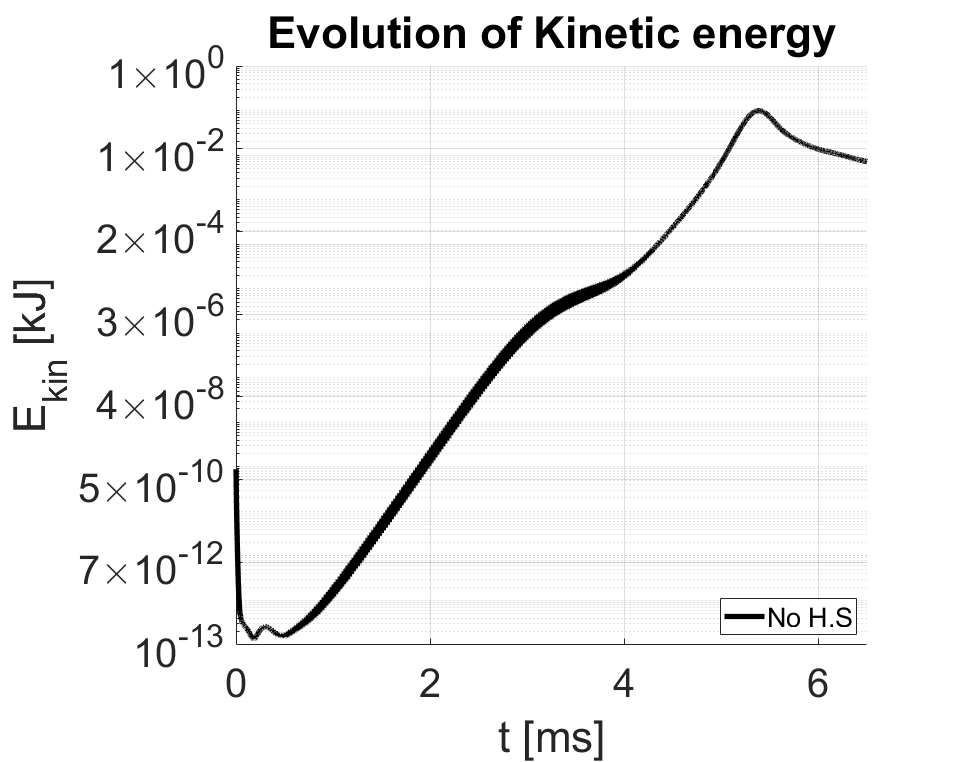
Figure 4: Evolution of kinetic energy of the spontaneous CDC event in LHD $\beta_{\rm axis}=4\%$ plasma using the $3$D non-linear non-adiabatic model

, without external heating source.

Figure 4 shows the time evolution of kinetic energy for the case without heat/particle source,$i.e$., $S_{\mathrm{n}}=0$, $S_{\mathrm{T}}=0$. The kinetic energy exponentially evolves during the linear stage, then the energy saturates and the plasma undergoes the CDC crash. The CDC event breaks the core density profile whilst maintaining the steep temperature and pressure profiles. Experimentally, a flattening of the density radial profile is observed [4, 11]. After the CDC crash, the plasma goes through the relaxation stage.

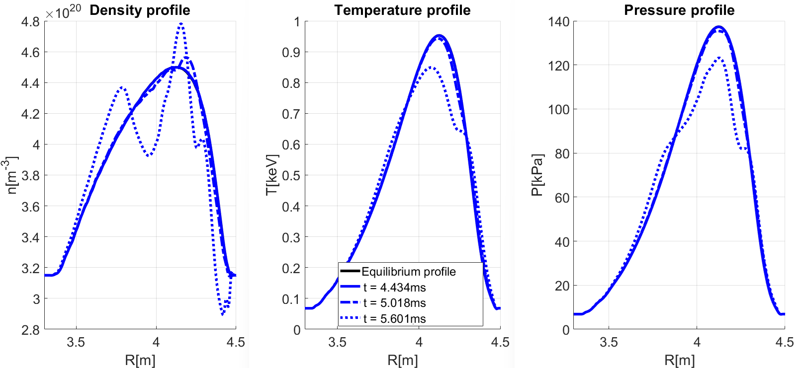
Figure 5: Radial profile versus major radius $(Z=$0\text{\,}\,\mathrm{m}$$, $\phi=(1/2)(2\pi/10))$ for density (left), temperature (center) and pressure (right). The results are obtained with $S_{\mathrm{n}}=0$, $S_{\mathrm{T}}=0$. Three time slices which correspond to the linear stage ($t=$4.434\text{\,}\,\mathrm{m}\mathrm{s}$$) with solid lines, near the CDC crash ($t=$5.018\text{\,}\,\mathrm{m}\mathrm{s}$$) with dash-dotted lines, and the relaxation stage ($t=$5.601\text{\,}\,\mathrm{m}\mathrm{s}$$) with dotted lines, are compared.

Figure 5 shows radial profiles versus major radius for density, temperature and pressure for the three time slices: linear stage ($t=$4.434\text{\,}\,\mathrm{m}\mathrm{s}$$), near the CDC crash ($t=$5.018\text{\,}\,\mathrm{m}\mathrm{s}$$) and the relaxation stage ($t=$5.601\text{\,}\,\mathrm{m}\mathrm{s}$$). The radial profiles are represented at the angle of the horizontally elongated poloidal slice, $\phi=(1/2)(2\pi/10)$ and $Z=$0\text{\,}\,\mathrm{m}$$ ($\simeq$ axis). The density profile collapse is observed, although it does not show the complete flattening of the profile expected from experimental results. However, the simulation represents the main characteristics of the CDC event, i.e. breaking of the core density profile whilst maintaining the steep temperature and pressure profiles. Further improvement of the model is required to be closer to the experimental observation for the future work. Density profile at the relaxation stage has a well near the boundary at the low field side of the plasma, $R\sim$4.4\text{\,}\,\mathrm{m}$$. This is due to the binary mask used for this work. In the binary mask region, $R>$4.5\text{\,}\,\mathrm{m}$$, density values does not change in time and it is set constant. The target physics to analyze in this work is the density collapse event in the core region, therefore the effect of binary mask location does not significantly affect the results. This numerical imprecision will be improved by refining the binary mask location and implementation in future work.

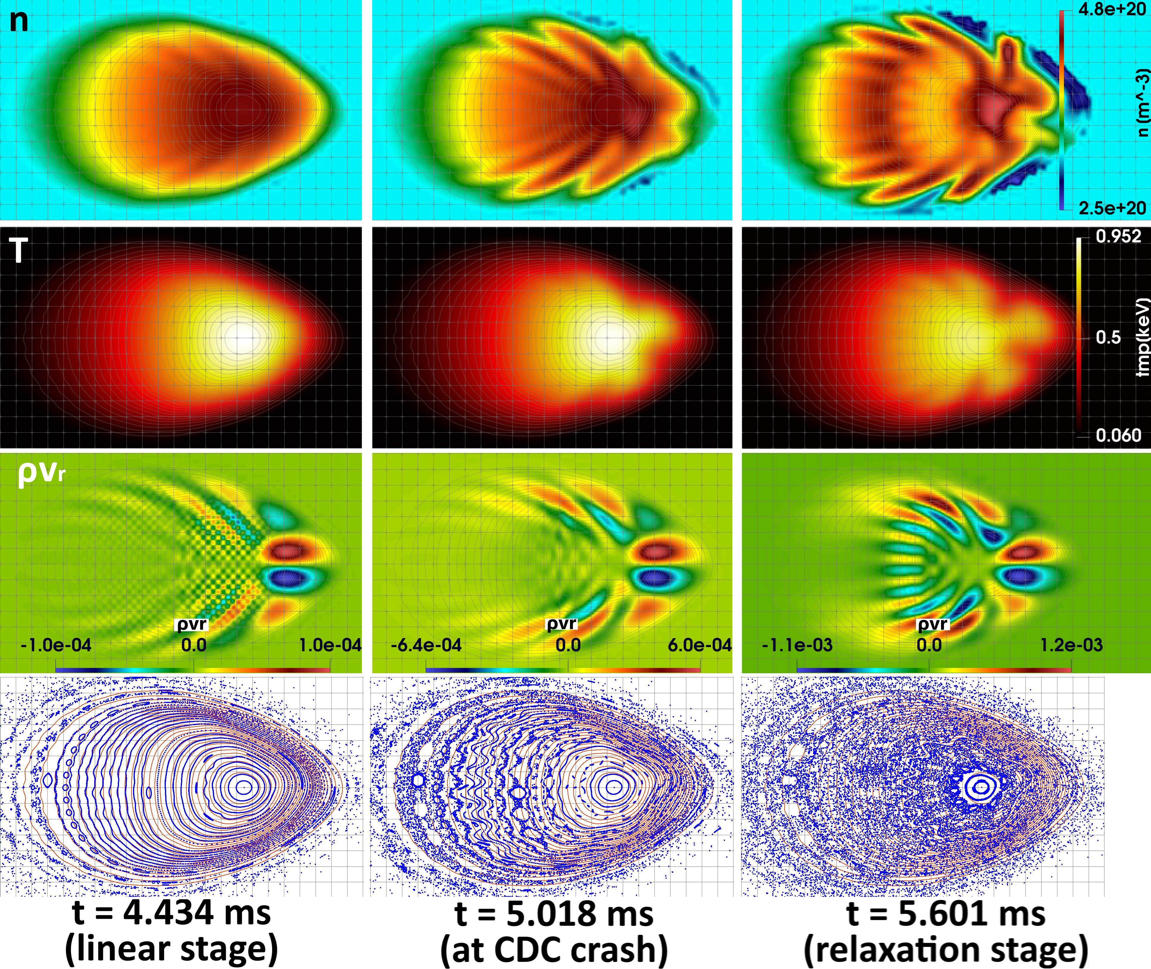
Figure 6: 2D contour plots at $\phi=(1/2)(2\pi/10)$ of density (top), temperature ($2$nd row), radial momentum ($3$rd row) and Poincaré plot (bottom) for the case without external source for three different time slices which correspond to the linear stage ($t=$4.434\text{\,}\,\mathrm{m}\mathrm{s}$$), near the CDC crash ($t=$5.018\text{\,}\,\mathrm{m}\mathrm{s}$$) and the relaxation stage ($t=$5.601\text{\,}\,\mathrm{m}\mathrm{s}$$). Equilibrium pressure contour lines are included in the figures for comparison in light gray for top, $2$nd and $3$rd rows, and in red for bottom row.

Figure 6 shows the 2D contour plots at the horizontally elongated poloidal slice, $\phi=(1/2)(2\pi/10)$ of density, temperature, radial momentum structures, and Poincaré plot. It shows the temperature profile is less affected while the density profile undergoes the collapse. The radial momentum profile shows a clear ballooning mode structure, which is known to be one of the triggering mechanisms of the CDC event [4, 2, 5, 12]. The Poincaré plot shows the fine magnetic flux surfaces in the linear stage. Then it becomes stochastic at the CDC crash and the stochasticity remains during the relaxation stage. There are some large magnetic islands generated at the CDC crash, then they are broken at the relaxation stage, where it becomes mostly stochastic. The evolution of stochastic region allows the plasma profiles to relax, and eventually the observation is consistent with the CDC event. The modeling of the CDC crash is observed to completely stochastize the magnetic field in W7-X [12] after the ballooning mode structure saturates. The nested topology is preserved in a region near the core, thus, the expected flattening of the density profile of the CDC event is not observed in this work.

3.3 Effect of external heat source on plasma response

In the following section of the study, the effect of an external heat source on the plasma response has been analyzed. The particle source is $S_{\rm n}=0$. The heat source is not included in the construction of the equilibrium, but it is added in the calculation of non-linear MHD evolution. In this work, two spatially different source profiles have been studied in order to understand the effect of the localization of the source: $1)$ toroidally uniform heating source $S_{\rm T,uni}$, and $2)$ toroidally localized heating source $S_{\rm T,loc}$. The sources are constant in time and have Gaussian profiles with the function of the normalized toroidal flux and toroidal angle, as described by:

$$S_{\rm T,uni}(\Phi_{\rm N}) =h_{0}\exp\bigg{(}{-\frac{(\sqrt{\Phi_{\rm N}}-\mu_{\Phi_{\rm N}})^{2}}{\sigma_{\Phi_{\rm N}}}}\bigg{)},$$ (15a)

$$S_{\rm T,loc}(\Phi_{\rm N},\phi) =S_{\rm T,uni}(\Phi_{\rm N})\exp\bigg{(}{-\frac{(\phi-\mu_{\phi})^{2}}{\sigma_{\phi}}}\bigg{)},$$ (15b)

where $$h_{0} \mu_{\rm\Phi_{N}}=0.0 \sigma_{\rm\Phi_{N}}=0.12 \mu_{\phi}=(1/2)(2\pi/10) \sigma_{\phi}=0.05$$ is the amplitude of the heat source. The heat source is centered at the magnetic axis, i.e. and has a width of . In the toroidally localized heating source case, toroidal location is set as , i.e. at the first horizontally elongated poloidal slice, and the width in the toroidal direction is .

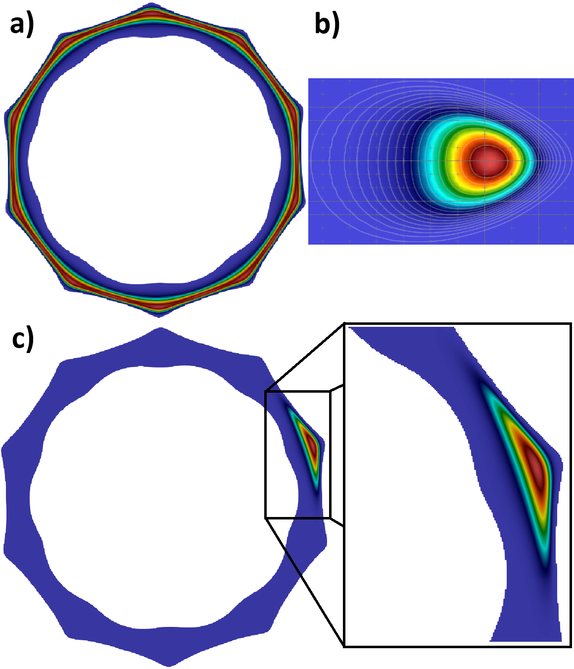
Figure 7: Heat sources profiles: a) toroidal heat source viewed at toroidal slice $Z=$0\text{\,}\,\mathrm{m}$$, b) poloidal cut of both toroidal and localized heat source at $\phi=(1/2)(2\pi/10)$ and c) localized heat source displayed toroidally at $Z=$0\text{\,}\,\mathrm{m}$$ (left) and zoomed in figure (box).

Figure 7 shows the profiles of the heating source at $Z=$0\text{\,}\,\mathrm{m}$$ for the two cases: 1) toroidally uniform heat source, 2) toroidally localized heat source. The peak of the source is centered at the magnetic axis so that the temperature profile grows in the core region. The aim of the work is to investigate the effect of the heating source; therefore, a Gaussian heating profile is assumed for this work. This source is expected to cause the pressure gradient to become steeper, therefore the CDC is expected to be triggered earlier than the spontaneous CDC event. The total injected power is computed as $H.S=\int_{\rm V}S_{\rm T}\,\rmd V$. A preliminary study for three different heat source amplitudes has been performed for $H.S=$1\text{\,}\,\mathrm{M}\mathrm{W}$,$6\text{\,}\,\mathrm{M}\mathrm{W}$$ and $10\text{\,}\,\mathrm{M}\mathrm{W}$.

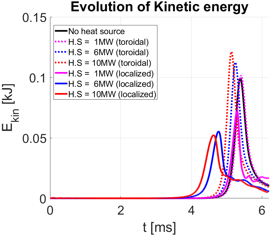
Figure 8: Kinetic energy evolution for the cases without heat source (black) for reference, with toroidal heat sources (dashed lines) and for localized heat sources (solid lines). The colors match the different heat source amplitude: $1\text{\,}\,\mathrm{M}\mathrm{W}$ (pink), $6\text{\,}\,\mathrm{M}\mathrm{W}$ (blue) and $10\text{\,}\,\mathrm{M}\mathrm{W}$ (red). The $\rm y$-axis is linear for clarity.

Figure 8 shows the time evolution of kinetic energies for i) spontaneous CDC event, ii) addition of toroidally uniform heating source, and iii) addition of toroidally localized heating source. The timing of the CDC event, which corresponds to the peak of the kinetic energy, occurs earlier in the cases of activated heating source. Increasing the heat source power contributes to cause the CDC event. The toroidally localized heating source triggers even earlier timing and smaller amplitude than the toroidally uniform heating source case.

Adding a toroidally uniform heat source increases both temperature and pressure profiles in the core region and it preserves the stellarator symmetry of the plasma profile. It enhances the pressure gradient in the core region, which triggers earlier the CDC event. Regarding the plasma profiles, the CDC event with toroidally uniform heating source case shows similar plasma evolution with the case without heating source, apart from the steeper pressure gradient.

Applying a toroidally localized heat source breaks the stellarator symmetry of the plasma configuration. For the same amount of integrated heating energy, the peak of the toroidally localized heat source is much larger than the one of the toroidally uniform heating source cases. The case $H.S=$6\text{\,}\,\mathrm{M}\mathrm{W}$$ has been chosen for the next studies.

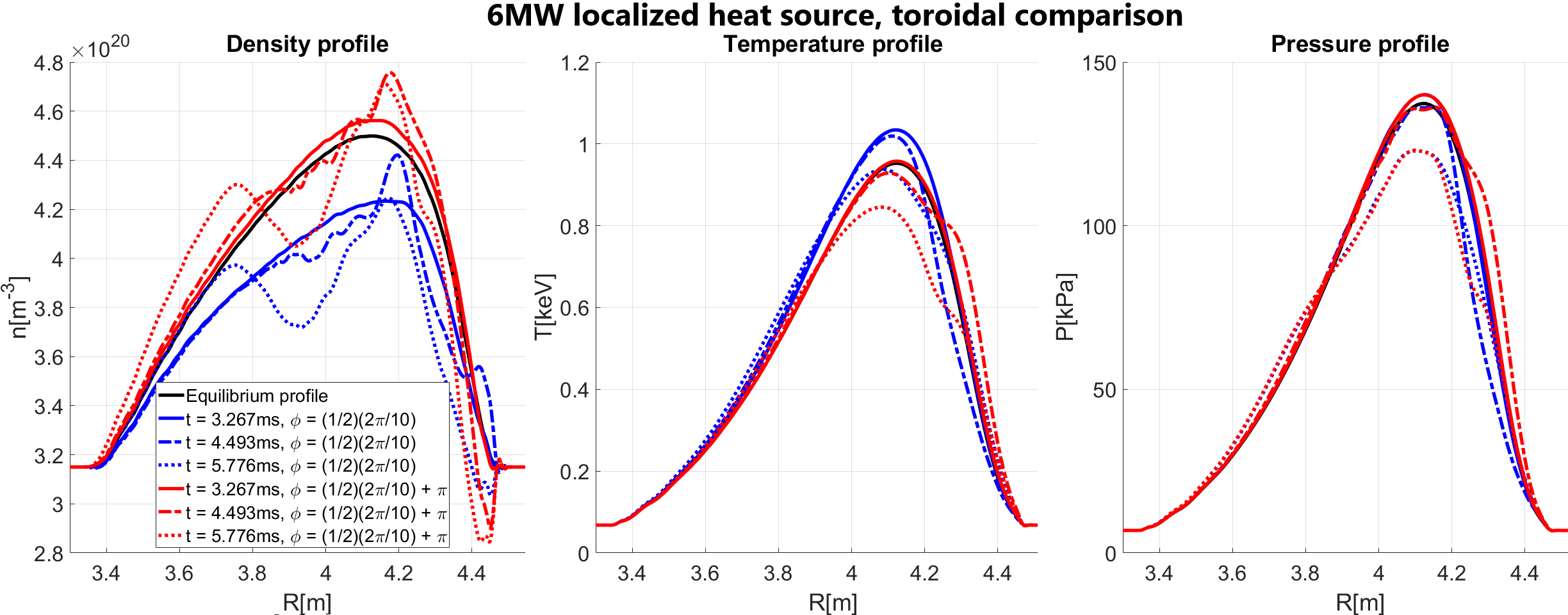
Figure 9: Radial profile versus major radius at $Z=$0\text{\,}\,\mathrm{m}$$ for density (left), temperature (center) and pressure (right), for the case of $H.S=$6\text{\,}\,\mathrm{M}\mathrm{W}$$ toroidally localized heat source. Three time slices are represented: linear stage ($t=$3.267\text{\,}\,\mathrm{m}\mathrm{s}$$) with solid lines, near CDC crash ($t=$4.493\text{\,}\,\mathrm{m}\mathrm{s}$$) with dash-dotted lines, and at the relaxation stage ($t=$5.776\text{\,}\,\mathrm{m}\mathrm{s}$$) with dotted lines. Two toroidal angles are represented: 1) $\phi=(1/2)(2\pi/10),$ which corresponds to where the heat source is centered (blue), and 2) $\phi=(1/2)(2\pi/10)+\pi,$ which is the toroidally opposite angle (red).

Figure 9 shows the evolution of the radial profile of density, temperature and pressure for the case of $H.S=$6\text{\,}\,\mathrm{M}\mathrm{W}$$ toroidally localized heat source. As consequence of the highly-peaked heat source, the local temperature in the core region and pressure gradient increase significantly while density decreases. On the other hand, at the opposite toroidal angle of the location of the heat source, the plasma temperature is practically unaffected while density grows. The increase of the steepness of the gradient at the location of localized heating source causes the CDC event even earlier than in the case of toroidally uniform heat source. Once the CDC event occurs, the plasma collapse appears over the whole plasma.

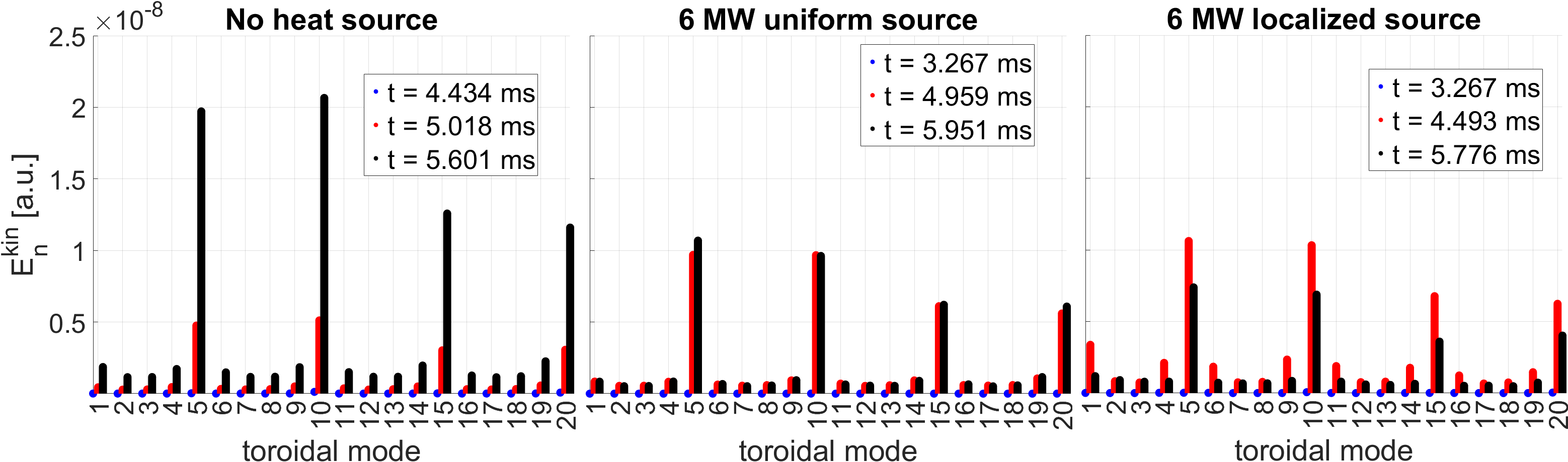
Figure 10: Toroidal mode spectrum amplitude of the kinetic energy for the case without heat source (left panel), with $6\text{\,}\,\mathrm{M}\mathrm{W}$ uniform heat source (middle panel), and with $6\text{\,}\,\mathrm{M}\mathrm{W}$ localized heat source case (right panel), for the three time slices corresponding to i) linear regime (blue), ii) near CDC crash (red), iii) relaxation stage (black).

Figure 10 shows the kinetic energy spectrum on boozer coordinates of the ${\rm n}=0-20$ toroidal modes, where a first average has been performed first over the ${\rm m}=0-30$ poloidal modes, and a second one over the normalized toroidal flux. Three time slices corresponding to i) linear regime, ii) near the CDC crash and iii) at the relaxation stage, for the case without any heat source, with $6\text{\,}\,\mathrm{M}\mathrm{W}$ uniform heat source, and the case with $6\text{\,}\,\mathrm{M}\mathrm{W}$ localized heat source are compared. The dominant modes of the kinetic energy spectrum are ${\rm n}=5,10,15,20$, for the three cases, as a consequence of the periodicity $5$ of the perturbation. The detailed discussion of the excited mode numbers of multiples of 5 is discussed in the next paragraph with Figure 11. The localized heat source excites not only toroidal modes ${\rm n}=5,10,15,20$, but also ${\rm n}=1$ due to the breaking of stellarator symmetry of the plasma. The localized heat source modifies the velocity field configuration through the non-linear process.

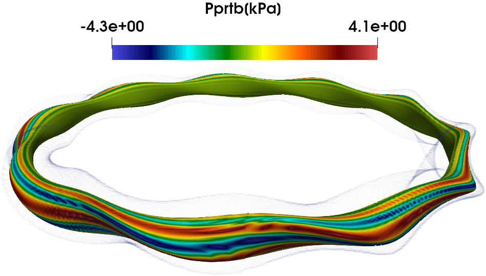
Figure 11: 3D contour plot of pressure perturbation (Pprtb) at the linear stage, $t=$4.434\text{\,}\,\mathrm{m}\mathrm{s}$$ of no-external heating source case. The pressure contour at $P=$8\text{\,}\,\mathrm{k}\mathrm{P}\mathrm{a}$$ with a light gray colored frame is shown for a reference.

Figure 11 shows the 3D contour plot of the pressure perturbation at the linear stage, $t=$4.434\text{\,}\,\mathrm{m}\mathrm{s}$$. The contour of the plasma at $P=$8\text{\,}\,\mathrm{k}\mathrm{P}\mathrm{a}$$ is represented as light gray for reference. The ballooning mode structure of the pressure perturbation is observed. The pressure perturbation profile has a toroidal periodicity of $5$ while the periodicity of the device is $10$. This is due to the magnetic field configuration, which is constructed using two helical coils of periodicity $5$. This periodicity of the perturbation contributes the toroidal mode numbers of ${\rm n}=5,10,15,20$, which appear frequently in the kinetic energy averaged spectrum structure evolution in Figure 10.

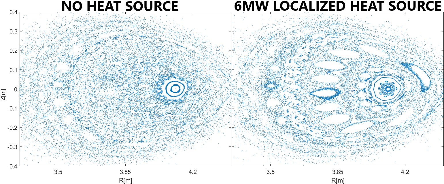
Figure 12: Poincaré plot at $\phi=(1/2)(2\pi/10)$ for the case without source (left) and the case with $6\text{\,}\,\mathrm{M}\mathrm{W}$ toroidally localized heat source (right) at the relaxation stage: $t=$5.601\text{\,}\,\mathrm{m}\mathrm{s}$$ (left) and $t=$5.776\text{\,}\,\mathrm{m}\mathrm{s}$$ (right).

Figure 12 shows the Poincaré plot at the relaxation stage and $\phi=(1/2)(2\pi/10)$ for the case without source and the case with toroidally localized heating source $6\text{\,}\,\mathrm{M}\mathrm{W}$. In the case of toroidally localized heating source, some magnetic islands grow after the CDC crash. The magnetic islands make the plasma profiles to flatten. The generation of magnetic islands implies the reformation of magnetic field configuration after the CDC event.

4 Conclusions and perspectives

The developed $3$D non-linear non-adiabatic MHD model, implemented in the MIPS code, allows to calculate anisotropic heat diffusivity and injection of particle and heat sources. The developed model has been benchmarked and confirmed the validity with the previous version of MIPS code. The 3D non-linear non-adiabatic MHD simulation shows preliminary results of main characteristics of CDC event observed in LHD plasma. The ballooning mode structures are observed before the CDC event. CDC event causes the drop of the density profile in the core region while temperature profile maintains the profile. The modification of the topological magnetic structure caused by CDC event has been observed, breaking the nested flux surfaces. The effect of heat source on the plasma response has been studied. The geometry of the added heating source, toroidally uniform heating source and toroidally localized heating source, has been compared. It has been observed that the amplitude and geometry of the external heat source have an influence on the MHD stability of the plasma. Adding external heating source is observed to enhance the pressure gradient in the core region, and consequently, triggering the CDC event earlier in time than the spontaneous CDC event, especially with the toroidally localized heating source case. The toroidally localized heating source excites the magnetic islands in its CDC event, more than the spontaneous CDC event. The observation implies that heating source can affect the magnetic field configuration. There are some discrepancies between the numerical results and experimental observations in terms of the plasma profile of post-CDC event. Future studies are expected to extend the physics model and numerical model to allow performing with more realistic plasma parameters in order to compare with experimental results.

References

Appendix A Table of denormalization of MIPS variables

Table 1: Definition of the variables used in MIPS code, and the normalization from/to SI units.

Magnitude	Variable	Unit	Dimensions	Denormalization
Length	$R,\vec{r}$	$[m]$	$[L]$	$\hat{r}$
Magnetic field	$\vec{B}$	$[T]$	$[MT^{-2}I^{-1}]$	$B_{0}\hat{B}$
Density	$n$	$[m^{-3}]$	$[L^{-3}]$	$n_{0}\hat{n}$
Mass density	$\rho$	$[kg/m^{3}]$	$[ML^{-3}]$	$\rho_{0}\hat{\rho}$
Pressure	$p$	$[N/m^{2}]$	$[ML^{-1}T^{-2}]$	$\frac{B_{0}^{2}}{\mu_{0}}\hat{p}$
Energy (Temperature)	$T$	$[J]$ or $[eV]$	$[ML^{2}T^{-2}]$	$\frac{B_{0}^{2}}{\mu_{0}n_{0}}\hat{T}$ or $\frac{B_{0}^{2}}{Z_{e}\mu_{0}n_{0}}\hat{T}$
Velocity	$\vec{v}$	$[m/s]$	$[LT^{-1}]$	$v_{A}\hat{v}=\frac{B_{0}}{\sqrt{\mu_{0}\rho_{0}}}\hat{v}$
Time	$t$	$[s]$	$[T]$	$\tau_{A}\hat{t}=R_{0}/v_{A}\hat{t}$
Current density	$\vec{J}$	$[A/m^{2}]$	$[IL^{-2}]$	$\frac{B_{0}}{\mu_{0}R_{0}}\hat{J}$
Resistivity	$\eta$	$[\Omega m]$	$[ML^{3}T^{-3}I^{-2}]$	$\frac{\mu_{0}R_{0}^{2}}{\tau_{A}}\hat{\eta}$
Kinematic viscosity	$\nu$	$[m^{2}/s]$	$[L^{2}T^{-1}]$	$\frac{R_{0}^{2}}{\tau_{A}}\hat{\nu}$
Particle diffusivity	$D_{\perp}$	$[m^{2}/s]$	$[L^{2}T^{-1}]$	$\frac{R_{0}^{2}}{\tau_{A}}\hat{D}$
Heat diffusivity	$\chi$	$[m^{2}/s]$	$[L^{2}T^{-1}]$	$\frac{R_{0}^{2}}{\tau_{A}}\hat{\chi}$
Particle source	$S_{\rm N}$	$[m^{-3}s^{-1}]$	$[L^{-3}T^{-1}]$	$\frac{n_{0}}{\tau_{A}}\hat{S}_{\rm N}$
Energy source	$S_{\rm T}$	$[W/m^{3}]$ or $[eV/m^{3}s]$	$[ML^{-1}T^{-3}]$	$\frac{B_{0}^{2}}{\mu_{0}\tau_{A}}\hat{S}_{\rm T}$ or $\frac{B_{0}^{2}}{Z_{e}\mu_{0}\tau_{A}}\hat{S}_{\rm T}$

In this work, the reference values used are: $B_{0}=$3.0\text{\,}\,\mathrm{T}$$, $n_{0}=$4.5\text{\times}{10}^{20}\text{\,}\,\mathrm{m}^{-3}$$, $\rho_{0}=n_{0}\times m_{p}~\mathrm{[kg\cdot m^{-3}]}$, $m_{p}=$1.672\,621\,92\text{\times}{10}^{-27}\text{\,}\,\mathrm{k}\mathrm{g}$$, $\mu_{0}=4\pi\times${10}^{-7}\text{\,}\,\mathrm{H}\mathrm{m}^{-1}$$, $Z_{\rm e}=$1.602\,176\,63\text{\times}{10}^{-19}\text{\,}\,\mathrm{C}$$ and $R_{0}=$3.6\text{\,}\,\mathrm{m}$$. The normalized values used in the numerical simulation are: Particle and perpendicular heat diffusivity, $D_{\perp}=10^{-7}$ and $\chi_{\perp}=10^{-5}$, respectively. Viscosity, resistivity and parallel heat diffusivity: $\nu_{\rm axis}=10^{-5}$,$\eta_{\rm axis}=10^{-5}$, $\chi_{\parallel,\rm axis}=10^{-2}$.

References

- [1] Ohyabu N, Morisaki T, Masuzaki S, Sakamoto R, Kobayashi M, Miyazawa J, Shoji M, Komori A and Motojima O (LHD Experimental Group) 2006 Phys. Rev. Lett. 97(5) 055002 URL https://link.aps.org/doi/10.1103/PhysRevLett.97.055002
- [2] Ohdachi S, Watanabe K, Tanaka K, Suzuki Y, Takemura Y, Sakakibara S, Du X, Bando T, Narushima Y, Sakamoto R, Miyazawa J, Motojima G, Morisaki T and Group L E 2017 Nuclear Fusion 57 066042 URL https://dx.doi.org/10.1088/1741-4326/aa6c1e
- [3] SAKAMOTO R, YAMADA H, OHYABU N, KOBAYASHI M, MIYAZAWA J, OHDACHI S, MORISAKI T, MASUZAKI S, YAMADA I, NARIHARA K, GOTO M, MORITA S, SAKAKIBARA S, TANAKA K, KAWAHATA K, KOMORI A, MOTOJIMA O and experimental group L 2007 Plasma and Fusion Research 2 047–047
- [4] S O, Sakamoto R, Miyazawa J, Morisaki T, Masuzaki S, Yamada H, Watanabe K, Jacobo V, Nakajima N, Watanabe F, Takeuchi M, Toi K, Sakakibara S, Suzuki Y, Narushima Y, Yamada I, Mianami T, Narihara K, Tanaka K, Tokuzawa T, Kawahata K and Group L E 2010 Contributions to Plasma Physics 50 552–557 URL https://onlinelibrary.wiley.com/doi/abs/10.1002/ctpp.200900051
- [5] Varela J, Watanabe K, Nakajima N, Ohdachi S, Garcia Gonzalo L and Mier J 2011 Plasma and Fusion Research 6
- [6] TODO Y, NAKAJIMA N, SATO M and MIURA H 2010 Plasma and Fusion Research 5 S2062–S2062
- [7] Suzuki Y, Nakajima N, Watanabe K, Nakamura Y and Hayashi T 2006 Nuclear Fusion 46 L19
- [8] Suzuki Y 2017 Plasma Physics and Controlled Fusion 59 054008 URL https://dx.doi.org/10.1088/1361-6587/aa5adc
- [9] Futatani S and Suzuki Y 2019 Plasma Physics and Controlled Fusion 61 095014 URL https://dx.doi.org/10.1088/1361-6587/ab34aa
- [10] Yamada I, Narihara K, Funaba H, Minami T, Hayashi H and Kohmoto T 2010 Fusion Science and Technology 58 345–351 (Preprint https://doi.org/10.13182/FST10-A10820) URL https://doi.org/10.13182/FST10-A10820
- [11] Sakamoto R, Yamada H, Kobayashi M, Miyazawa J, Ohdachi S, Morisaki T, Masuzaki S, Goto M, Funaba H, Yamada I, Ida K, Morita S, Peterson B J, Ohyabu N, Komori A and Motojima O 2010 Fusion Science and Technology 58 53–60 URL https://doi.org/10.13182/FST10-A10793
- [12] Suzuki Y, Futatani S and Geiger J 2021 Plasma physics and controlled fusion 63 124009:1–124009:2 URL http://hdl.handle.net/2117/357620