Ivan Biočić
, Daniel E. Cedeño-Girón
and Bruno Toaldo
Abstract.
In this paper, a method to exactly sample the trajectories of inverse subordinators (in the sense of the finite dimensional distributions), jointly with the undershooting or overshooting process, is provided. The method applies to general subordinators with infinite activity. The (random) running times of these algorithms have finite moments and explicit bounds for the expectations are provided. Additionally, the Monte Carlo approximation of functionals of subdiffusive processes (in the form of time-changed Feller processes) is considered where a central limit theorem and the Berry-Esseen bounds are proved. The approximation of time-changed Itô diffusions is also studied. The strong error, as a function of the time step, is explicitly evaluated demonstrating the strong convergence, and the algorithm’s complexity is provided. The Monte Carlo approximation of functionals and its properties for the approximate method is studied as well.
Key words and phrases:
Inverse subordinators, anomalous diffusion, time-changed processes, semi-Markov processes, Monte Carlo method
2020 Mathematics Subject Classification:
60K50, 65C05
The authors acknowledge financial support under the National Recovery and Resilience Plan (NRRP), Mission 4, Component 2, Investment 1.1, Call for tender No. 104 published on 2.2.2022 by the Italian Ministry of University and Research (MUR), funded by the European Union – NextGenerationEU– Project Title “Non–Markovian Dynamics and Non-local Equations” – 202277N5H9 - CUP: D53D23005670006 - Grant Assignment Decree No. 973 adopted on June 30, 2023, by the Italian Ministry of University and Research (MUR)
The authors would like to thank the Isaac Newton Institute for Mathematical Sciences, Cambridge, for support and hospitality during the programme Stochastic systems for anomalous diffusion, where work on this paper was undertaken. This work was supported by EPSRC grant EP/Z000580/1
1. Introduction
The interplay between continuous time random walks (CTRWs), time-changed Markov processes and fractional-type non-local equations gained considerable popularity in the last decades. This is certainly connected to the central role that this theory has for modeling anomalous diffusion, especially in the context of Hamiltonian chaos [83; 84; 85], Hamiltonian systems describing cellular flows [37; 38], trapping models [2; 76], anomalous heat conduction [26; 70], option pricing [42], neuronal modeling [4], and many others, see e.g. [10; 11; 27; 28; 29; 34; 63; 64; 67], and references therein for several possible applications and modeling aspects of the theory.
One of the milestones in this context is the seminal paper [66] from which the CTRWs were rapidly adapted and tested for their suitability to describe anomalous diffusions in carrier transport in amorphous solids [77; 78; 79].
A CTRW in describes the motion of a particle performing independent random jumps paced by independent residence times. In formulae: If is a sequence of non-negative absolutely continuous independent identically distributed random variables (residence times), then a CTRW is defined as the process given by
(1.1)
Here is a sequence of independent identically distributed random variables in and .
CTRWs lead, after a scaling limit, to fractional partial differential equations (PDEs) under appropriate assumptions on the non-exponential residence times and the jumps. In practice, one can introduce a scale parameter to get a scaled process that converges as (in a suitable sense) to another process such that solves the fractional equation
(1.2)
with . Here is the fractional derivative in the Caputo sense, i.e.
(1.3)
and is a linear operator connected to .
Hence, since very often CTRWs can be simulated exactly, a lot of efforts have been dedicated to approximations of solutions to fractional PDEs using Monte Carlo methods based on CTRWs, see e.g. [30; 35; 82] and the references therein. The recent work [52] also provides convergence rates for functional limit theorems for CTRW approximations to the fractional evolution. We also note that CTRW approximations have an effective alternative in numerical methods, see [56].
It turns out that the CTRWs limit processes are time-changed Markov processes. More precisely, define and suppose that , as , weakly in the space of càdlàg functions endowed with the Skorohod topology, where is a Feller process. Then where , see [62, Section 2]. Note that when and are independent, one has that a.s. Moreover, the processes are subdiffusive in the sense that the process , used as a time-change, induces intervals of constancy whose duration is arbitrarily distributed (depending on the jumps of ), and as such are suitable to model sticking or trapping effects in an evolution. The mean square displacement for these processes has been studied in several cases (see, e.g., [49; 81]) and shown to be sublinear.
The stochastic representation of the solution to (1.2) is obtained by assuming that is a Markov process with the infinitesimal generator , and by assuming that is a positively skewed stable process (i.e. a stable subordinator) independent of , see [8]. If is a general subordinator independent from , then the governing equation is as in (1.2) but with a different non-local time operator as in (4.10), see e.g. [18; 40; 50; 51; 61]. The process is then called an inverse subordinator (or local time), see more on these processes in [5; 12]. If the random variables and (the residence time and the subsequent jump) are not independent, then the processes and are not independent. In this case, the governing equation is non-local in both variables and in a coupled way, i.e. the non-local operator acts jointly on both variables and , see [6; 9].
In light of this relationship between fractional PDEs and subordinators, simulating and inverting subordinator paths raised a new strategy to solve non-local PDEs numerically, see e.g. [45; 59; 60]. The papers [36; 43; 45; 48] provided a framework for connecting Itô diffusions time-changed with inverse subordinators and their associated transition densities, where approximations of these processes and the convergence rate were also studied.
In these papers, however, the paths of inverse subordinators were always simulated approximately, from the trajectories of the corresponding subordinator.
The exact sampling of the inverse subordinator has been done exactly, only for a fixed single time and in the stable case, in the paper [53], where the Monte Carlo estimator for the stochastic representation of the solution to the fractional Cauchy problem was studied. Also, very recently, in [24] the authors show a paths’s approximation for Lévy processes time-changed by inverse subordinators using a martingale approach (see Section 7 there).
Clearly, a method to make exact samples of trajectories of an inverse subordinator (i.e. a method for exact sampling from the finite-dimensional distribution) would be crucial in the context of modeling diffusion subject to sticking or trapping, and for approximating the associated non-local kinetic equations. With the so far developed techniques it is impossible to perform this sample exactly, but only using approximations from the paths of the subordinator, and in some specific cases. However, the single time exact sampling of the inverse subordinator is already possible using different techniques. This has been done in [19; 21] for stable subordinators and their truncated and tempered versions, and in [32; 33] which are the more general and up-to-date contributions. The latter papers, provide an exact and fast algorithm to sample a quite general class of inverse subordinators, at a fixed single time. This will be the starting point for the algorithms developed in this paper.
1.1. Main results and structure of the paper
In this work we develop a method to make exact samples from the finite-dimensional distributions of the processes
Here is the inverse of the strictly increasing subordinator , where is called the age process, and is called the remaining lifetime process. The processes and are called the undershooting and overshooting of the subordinator, respectively. Our method can be applied to any inverse subordinator even with infinite activity. However, the algorithm requires exact sampling from the single time distribution of the processes , and . This is currently possible for a fairly general class of inverse subordinators, using the method described in [32; 33]. The sampling of trajectories is detailed in Section 3, and the procedures are given in Algorithms 1 and 2. The computational complexity is also provided explicitly in Proposition 3.5.
With this at hand, we then study some properties of a Monte Carlo estimator for the quantity , where is an arbitrary Feller process in , denotes the expectation when a.s., and are suitable functionals, for arbitrary and any choice of times . For the Monte Carlo estimator we prove, in particular, a Central Limit Theorem (CLT) and the Berry-Esseen bounds, see Theorem 4.3. This is detailed in Section 4.
The previously discussed Monte Carlo method is applicable whenever the Feller process can be sampled exactly. This is of course not always possible. In Section 5, we consider an Euler-Maruyama scheme for the approximation of the trajectories of time-changed Itô diffusions. In particular, we provide an estimate for the strong error as a function of the time step of the scheme, and as a consequence the strong convergence order is determined. Our method improves classical methods in the literature, e.g. [48], as we avoid the error in the scheme introduced by approximation of the paths of the inverse subordinator.
With this at hand, we then consider a Monte Carlo estimator for functionals of the approximate process: properties, such as a CLT and computational complexity, are then studied.
In the next section, we provide some preliminary notions and a description of some already existing algorithms that are relevant to our paper.
2. Exact sampling and computational complexity
We start by explaining what we mean by an exact simulation. For this notion, we suggest the instructive discussion in [33, Appendix D] to which we refer to the notion of exact (or practically exact) simulation adopted in this paper. For the reader’s convenience, here we summarize the main parts.
Since computers dispose of finite resources (bits of precision) the law of the output of any algorithm will differ from the target law. The more intuitive notion of exact simulation, useful in practice, is the following: A simulation is exact if the distance (associated with a suitable metric) between the desired and simulated law is controlled with machine precision, i.e. with bits of precision. In other words, if is the ideal simulated quantity and denotes the output of the simulated law, determining if the simulation is exact reduces to check a suitable distance , where denotes the law of the corresponding quantity. The choice of the metric is clearly crucial in this context. Several distances might be taken into account but the obvious one is the Wasserstein distance which, however, shows its limitations even in the context of a rejection sampling, see, in particular, [33, Item I, Appendix D]. Here we will consider the Lévy-Prokhorov metric. The latter metrizes weak convergence and in this sense it is a very natural choice; its definition is as follows. For two given probability measures and on a metric space , define the distance , where , which is called the Lévy-Prokhorov distance between and . Let be the family of probability measures on such that each has marginals and , respectively. Then, it is true that (see [25] for details)
(2.1)
i.e. the distance is the smallest such that the distance between and is no more than under a suitable law , with probability at least .
Then, in the case of an algorithm that employs times numerical methods of the -th kind, each one controlling the error in the quantity , the Lévy-Prokhorov distance is bounded by . In this paper we adopt this notion of exact simulation (or, practically exact according to [33]): we say that an algorithm is exact if the above distance between the output and the ideal variable can be controlled with the machine precision, i.e. if , where is a constant (that can be determined explicitly) and is the number of bits of precision.
Our algorithms will not be constructed using approximations, but their implementation might require to call others that do so. In particular, the implementation of our Algorithm requires to sample from (the single time) distribution of . In [33], the authors provided a method to do so in the case when is a tempered stable subordinator, i.e. its Lévy density is
(2.2)
for some and , where is the Lévy density of the -stable subordinator. The method is then generalized to more general subordinators by the same authors, see below and [32].
The method from [33], called the TSFFP-Algorithm, returns exact samples of the first passage event (i.e. the first-passage time, undershoot, and overshoot) across an absolutely continuous non-increasing function, called the barrier. Hence, it can be used to get an exact sample of the vector at fixed time . The provided method is exact in the sense above, despite employing numerical inversion and integration, see Appendix D.1 in [33] where the authors prove exactness in the Lévy-Prokhorov metric. In fact, the TSFFP-Algorithm reduces the complexity of dealing with a tempered stable subordinator to a non-tempered one by the Esscher transform. An additional rejection sampling step is then required to obtain the first passage event of the tempered stable subordinator from the stable one. In turn, sampling the first passage event of a stable process relies on sampling from the undershoot law, since the first-passage time and the overshoot laws are explicit. The undershoot law implies the stable law, which involves a non-elementary integral. This latter is circumvented by extending the state space and using modified versions of the rejection sampling method, such as [54; 55]. For more details, see [33, Sections 2.4 and 4.3].
The generalization is [32, Algorithm-1] which is the extension of the algorithm in [33] to a larger class of subordinators. The available class of subordinators is such that their Lévy density satisfies as , where . Here as stands for , where and are positive functions. In such cases, the Lévy density can be written as
(2.3)
for some constants , , , and a density of a finite measure on . For further details see [32, Appendix A]. Here we also mention that can be changed to the condition , for any constant . Indeed, the multiplication of the Lévy measure by a constant only changes the time scale of the subordinator. At the end of the next section, one can find examples of such subordinators as well as the simulations of their trajectories.
To the best of our knowledge, the two algorithms mentioned above are the only ones that return exact (in the sense above) samples of the first passage event of a subordinator.
The implementation of the algorithm in our paper requires running the algorithms above a finite (explicit) number of times and adding some elementary arithmetic operations or rejection sampling. Therefore, the error propagation is easily controlled as, at the end of our algorithm (end of the trajectory), the error is bounded by the error made in [33, TSFFP-algorithm] or [32, Algorithm-1], which can be controlled with machine precision times a finite number (that can be determined by the number of iterations and elementary operations).
To be precise, the Lévy-Prokhorov distance between the desired and simulated random variable is bounded by the maximum number of iterations between the numerical methods employed, multiplied by the desired error tolerance. In the case of the TSFFP-Algorithm, the Lévy-Prokhorov distance is bounded by , where , and are parameters of the problem, , and is the number of bits of precision, see [33, Appendix D.1] for this estimate.
2.1. Computational complexity
We remark that, since the two mentioned algorithms from [33; 32] are fast, see the discussion in [33, Section 2.2], and we perform a finite number of iterations and elementary operations, our algorithms are fast in the same sense as well.
Computational complexity refers to the resources needed by an algorithm to complete its task and is usually expressed as a function of the inputs of the algorithm, see [20]. Here, we focus on the computation time, also known as running time, which encompasses the number of instructions executed and data accesses performed during the algorithm’s execution. Additionally, if an algorithm incorporates an element of randomness, its computational complexity becomes random as well, so it is also meaningful to study the moments of the (random) running time.
Here we present the complexity of [32, Algorithm-1], which is relevant since we will use it to determine the complexity of our algorithms which will be given in Propositions 3.5, 4.1, 5.6, and 5.8. The running time of [32, Algorithm-1], according to Theorem 2.1 therein, has moments of all order and its first moment is bounded above by
(2.4)
Here is a constant that does not depend on parameters , , , , , or , , while for and , we have
(2.5)
Finally, stands for the expected running time of [33, Algorithm TSFP] which bound is given in [33, Theorem 1] and reads
(2.6)
where is a constant that does not depend on the above parameters, is the target barrier at time zero, and specifies the required number of precision bits of the output.
The expressions (2.4) and (2.6) were obtained by assuming that elementary operations (such as addition, multiplication, definition of objects, and evaluation of functions, among others) have the same cost of one. This assumption is adopted herein, and for the sake of brevity, we will refer to the complexity (random running time) of [32, Algorithm-1] and its first moment as and , respectively, throughout the document; hence is bounded by (2.4).
3. Exact simulation of paths of the inverse, undershoot, and overshoot of a subordinator
In this section, let be a subordinator, i.e. an increasing Lévy process with , with the Laplace exponent given by
(3.1)
with infinite activity, i.e. , and a potentially positive drift . There is one-to-one correspondence between functions of type (3.1) and subordinators, see [80]. The infinite activity means that the subordinator has a countable infinity of jumps in any given finite time interval.
We denote the inverse of by , where , the undershooting of by where , and the overshooting by , where .
The method provided in [32], described in Section 2, gives the possibility to make exact simulations of the vector for a fixed and a quite general class of subordinators. Furthermore, since subordinators start at zero, one has that almost surely, and thus the method above does not allow to sample under different starting points. Denote by and . In this section, we provide a method of exact simulation of the trajectories and , in a finite (but arbitrary big) number of points, when the process can start at . In other words, we can assume any starting point and , with , , . In practice, we furnish a method to exactly sample the vectors
(3.2)
and
(3.3)
for any choice of , , and without assuming or . Since the starting point of the subordinator is , a.s., one has that and , hence in order to give a meaning to the event we perform the following construction of the mentioned processes.
Take the Feller semigroup , , acting on functions , given by
(3.4)
where denotes the Dirac point mass at , and is the one-dimensional distribution of the subordinator with the Laplace exponent (3.1). In particular, this is a convolution semigroup induced by a Lévy process, see e.g. [15, Examples 1.3 and 1.17], denoted by , where is a pure drift, and is an independent subordinator, both not necessarily started at zero. We construct this process as the canonical one in the sense of [73, Chapter III.1], and thus on the filtered probability spaces where is the natural filtration, , and is the (unique) probability measure such that .
Now, we can define, as above, the processes , and , paying attention that under one has that , and , while under for , one could have different starting points and thus is the inverse of a subordinator started at and and are the corresponding undershooting and overshooting.
It turns out that the process has a certain kind of semi-Markov property. In particular, it turns out that , has the simple Markov property and can be inserted in the theory developed by [62, Section 4]. For a general discussion of definitions of semi-Markov properties, see [39, Chapter III]. We can apply the theory of [62, Section 4] also to the process , and it turns out that is a Hunt process, i.e. it is a strong Markov càdlàg process which is quasi-left-continuous. In following paragraphs, we formalize the previous assertions.
It is clear that under the processes , , and are just the inverse of a subordinator, the so-called customary age, and the so-called remaining lifetime process, respectively, while is just the process . First recall that is the inverse of a strictly increasing subordinator (started at an arbitrary point), so it has continuous trajectories (and so does ). It is easy to see that the process is right-continuous, while the age process is left-continuous.
The discontinuity points of the process , occur at times in the range of that are isolated on their left, i.e. in times , where . Hence has no fixed discontinuities, and a.s. for any provided that . In practice, this implies that if we consider the right-continuous version
(3.5)
then we have , -a.s., for all fixed . However, conditioning on , under with , there could be a positive probability that is a discontinuity point of , e.g. if the Lévy measure has a mass. Therefore, we will focus here on the customary left-continuous process .
We first formalize the (simple) Markov property of the process , and then the strong Markov property of , .
Theorem 3.1.
The process , is a homogeneous Markov process with the transition probabilities satisfying
(3.6)
(3.7)
for all and .
Proof.
To prove the result we resort to [62, Theorem 4.1].
From the Fourier symbol
(3.8)
where is the Bernstein function (3.1) associated with , and by using [75, Theorem 31.5], it
is plain that the semigroup , , is generated by such that
(3.9)
where is the Lévy measure of the subordinator (i.e., it is supported on ). It follows that our process is (also) a jump diffusion in the sense of [1] and also in the sense of [62], i.e. the generator (3.9) has the form of [62, Formula (2.5)] with the jump kernel
(3.10)
Recall that the process , generates the semigroup , , where the first coordinate is a pure drift, and that is the inverse of the second coordinate . Thus, satisfies . The result then follows by an application of [62, Theorem 4.1]. Indeed, this theorem says that is a homogeneous simple Markov process associated with a semigroup of operators , , on the space of bounded Borel functions, such that for it holds that
(3.11)
(3.12)
from which it follows that
(3.13)
(3.14)
(3.15)
where we also used (3.10).
In order to apply [62, Theorem 4.1], one should check that the process associated with , , is Markov additive in the sense of [17], i.e. that the future depends only on the current state of , but in our case this is clear since is a Lévy process started at .
∎
Now we formalize the strong Markov property of , .
Theorem 3.2.
The process , , is a Hunt process with the transition probabilities satisfying
(3.16)
for all and .
Proof.
The proof follows similarly as the one of Theorem 3.1. Indeed, [62, Theorem 3.1 & Theorem 4.1] imply that is a Hunt process associated with a semigroup of operators , , on the space of bounded Borel measurable functions such that
From Theorems 3.1 and 3.2 it is clear that we can use the simple Markov property to obtain our algorithm for the exact sampling of paths of and . Indeed, denote by
(3.21)
(3.22)
the distribution of vectors (3.2) and (3.3) for , conditioning on and .
Then, by Theorem 3.1 we have that, for , ,
Here we show that we can sample from the transition probabilities appearing in (3.23) and (3.24). We do this by showing that there exists r.v.’s whose distributions under are given by such probabilities, with an appropriate choice of parameters.
Proposition 3.3.
Consider a family of random variables , , with the distribution, under ,
(3.25)
with the parameter , independent from and a random vector
(3.26)
with the parameters , , , .
Let be the transition probabilities defined in Theorem 3.1. Then it holds that
(3.27)
Furthermore, let
(3.28)
then
(3.29)
Proof.
Under , the process is a subordinator with a.s., and is the inverse of , so and , a.s. It follows that
(3.30)
where we used the independence between and , the form of the distribution of and the fact that as explained above. The result follows by observing that (3.30) coincides with the transition probabilities obtained in Theorem 3.1.
The second result follows immediately by Theorem 3.2.
∎
The previous proposition, together with a simple conditioning argument, suggest the following result.
Proposition 3.4.
Let be an arbitrary probability space supporting , and , , that are independent copies of the random variables introduced in Proposition 3.3.
It is true that
(3.31)
where , , and, for ,
(3.32)
Further, it is true that
(3.33)
where , , and, for ,
(3.34)
Proof.
Since the probability space here is inessential, the proof follows by a simple conditioning argument and Proposition 3.3.
∎
The random variables and appearing in Propositions 3.3 and 3.4 are easily exactly simulated provided that falls in the class of subordinators for which we can exactly sample , see Section 2, and that we can sample . This inspires the Algorithms 1 and 2 which give a method to exactly sample the random vectors
(3.35)
(3.36)
for any choice of , . Note again that, since is pure drift started at under , the processes is just the inverse of the second coordinate , translated by .
Algorithm 2generating vectors (3.36) conditionally on ,
Recall that denotes the (random) running time of the algorithm [32, Algorithm-1], and denotes its expectation, for details see Section 2.1.
Proposition 3.5.
Let be the number of time points and let , , denote a sequence of i.i.d. random variables with the distribution of , and define . If the inverse of the cumulative density function of the random variable is known explicitly, then the Algorithm 1 has complexity , with the mean running time bounded by and finite moments of all order. The Algorithm 2 has the complexity with the mean running time bounded by and finite moments of all order.
Proof.
Let us start by analyzing Algorithm 2 first. In it, the lines 2, 3, 4, 7, and 8 correspond to the worst case, since they contain the largest number of computations and also perform the call to [32, Algorithm-1]. The lines 2, 3, and 8 have the cost of one, as assumed in Section 2.1, and are executed times. Line 7 has the complexity of , with a mean value bounded by (2.4), and is (independently) executed times. The claim for Algorithm 2 now easily follows.
In the case of the Algorithm 1, the lines 2, 3, 4, 8, 9, 12, and 13 represent the least favorable scenario. The line 12 has the complexity , and the line 8 has the cost of two by the assumption that the inverse of the cumulative density function is known. The latter holds true since the line 8 first generates a uniform random variable and then evaluates the inverse cumulative density function to get the sampled random variable . The remaining lines have the cost of one, as only elementary operations are performed and each is executed times. This finishes the proof.
∎
Remark 3.6.
It is clear that if one only wants to sample the trajectory of , it is more convenient to use Algorithm 2 as it does not require sampling the random variables . We remark that the idea of using the overshooting to make a process Markovian and simulate its trajectories has been already used, in a different context, i.e., for a discrete time process, in [65].
Remark 3.7(On sampling paths of tempered subordinators).
Let be an absolutely continuous Lévy measure and its tempered version, i.e. , . If samples of the random variable with the distribution as in (3.25) are available, then samples of the tempered version, denoted here by , are also available through the rejection sampling method.
Recall that the rejection sampling method consists of sampling random variables from a target distribution with a probability density function using a proposal distribution with a probability density function . The idea is to generate random variables from the distribution and accept them with probability . The constant represents a finite value that serves as a bound of the likelihood ratio over the support of , see [7, p. 39]. In our case, is
(3.37)
In other words, to obtain samples of , first we generate samples and from and , respectively, and accept the value if .
An example is the tempered stable Lévy measure. In this case,
(3.38)
where , , and represents the Gamma function. Furthermore, the cumulative distribution function of , denoted here by , and its inverse are available. Indeed, we have . Therefore, samples of random variables with distribution can be obtained through the inverse transform sampling method [7, p. 37]. This allows us to sample the paths of the -stable inverse subordinator along with the undershoot and overshoot processes and their respective tempered versions using Algorithms 1 and 2.
Example 3.8.
In addition to the stable subordinator and its tempered version, Section 4.2 of [32] provides an illustrative example. Another example can be found in [80, p. 307], where the Lévy measure and the Laplace exponent of the subordinator are , , , and , respectively. Note that by setting we have
(3.39)
where we use the fact . Then it is clear that as .
Thus, the assumptions of [32, Algorithm-1] are satisfied, see the discussion in Section 2. In order to apply our algorithm, one should also have the distribution of the random variable . However, the tail of is known explicitly .
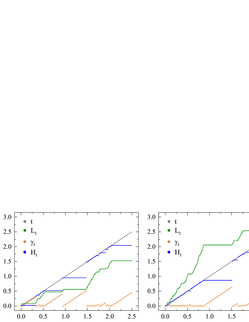
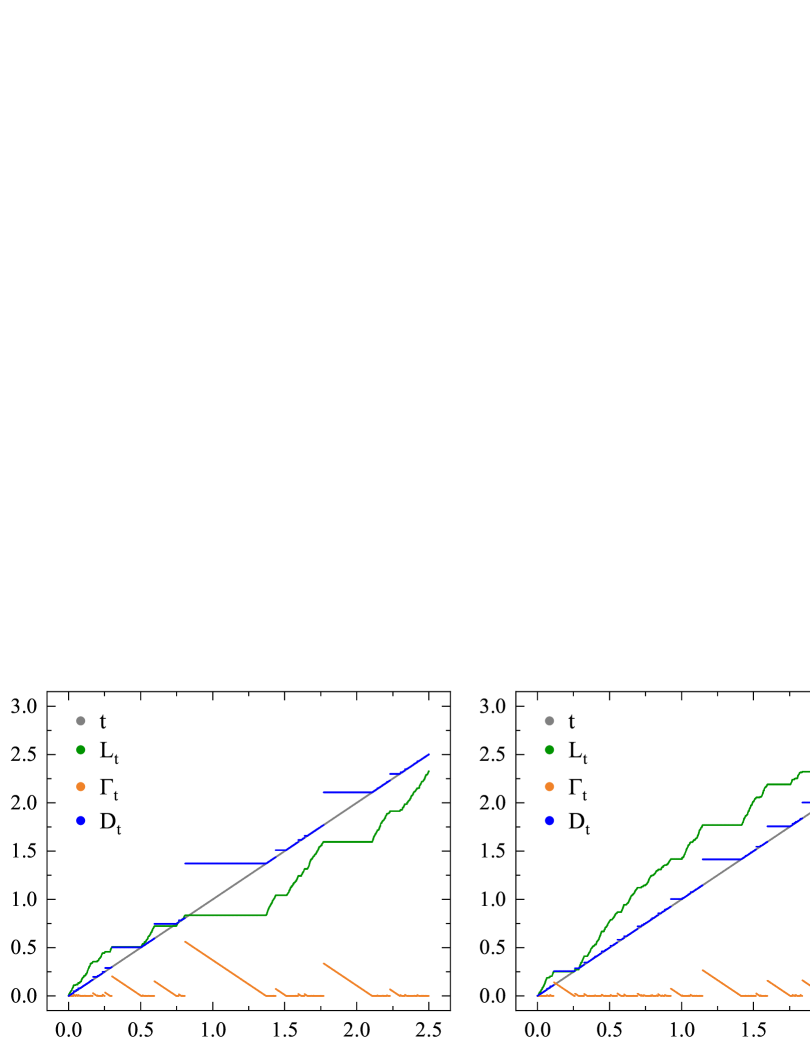
For illustrative purposes, we look at the -stable subordinator and its tempered version, see Figure 1. We attach the GitHub repository with the Python code used to sample figures for the reader’s convenience [13].
(a)Sample of the -stable inverse subordinator, age process, and undershoot process through Algorithm 1, left figure, while the right one stands for the tempered version.
(b)Sample of the -stable inverse subordinator, remaining lifetime process, and overshoot process through Algorithm 2, left figure, while the right one stands for the tempered version.
Figure 1. Paths for the -stable inverse subordinator and its tempered version in a time interval from to with equidistant steps with , , and . The green, orange, and blue colors stand for the inverse subordinators, age process (remaining lifetime), and undershooting (overshooting) process, respectively. Time is displayed in black.
4. Exact simulation of time-changed processes and Monte Carlo method
The ability to make simulations of the vectors (3.2) and (3.3) yields the possibility of exact sampling of the trajectories of suitable time-changed processes.
Namely, consider a Feller process , , on .
As long as it can be sampled exactly, its composition with an independent inverse subordinator, its undershoot, or its overshoot (sampled as shown in the previous section) can be also sampled exactly.
Here is the construction of the process we are going to sample.
Consider the canonical construction of the process , where is a Feller process and is an independent strictly increasing càdlàg process with stationary and independent increments. Hence, we have the (family of) filtered probability spaces where is the natural filtration, , and is the unique measure such that . In particular, we have that defined as is a subordinator under any while is a subordinator under . Define now the first-passage processes
Recall that since is assumed to be strictly increasing then the inverse is, a.s., continuous.
We define
In particular, under , is a subordinator, is the undershooting and the overshooting.
Following [6, Section 4] it is possible to prove that the processes
(4.1)
(4.2)
are Markov additive processes in the sense of Cinlar [17] on the probability spaces above. Therefore, it is noteworthy that whenever the Feller process (4.1) is a jump diffusion it can be inserted in the theory developed in [62, Section 4], i.e. the left-continuous process has the simple Markov property, while is a Hunt process. Equivalently, if the process (4.2) is a jump diffusion, then the left-continuous process has the simple Markov property while is a Hunt process.
To summarize, by using the results of the previous section we can make exact sampling of the vectors
(4.3)
(4.4)
(4.5)
under , for any , . Here is a subordinator with the Laplace exponent (3.1), is its inverse process, is the undershooting of the subordinator, while is the overshooting of the subordinator . This is possible whenever an exact algorithm to make simulations of the Feller process is available, as shown in Algorithm 3. We use for the inverse subordinator or the undershoot process , or the overshoot process , of a given subordinator , where no distinction between the three is needed.
Algorithm 3Generating vectors (4.3), (4.4) and (4.5) under
Examples of Feller processes whose trajectories can be sampled exactly include for example the following processes. Diffusions for which an analytical solution is known constitute one example, see e.g. [47, Section 4.4] which offers many such examples. In the context of diffusion processes, we highlight the class of one-dimensional diffusions that under specific conditions of the drift and the diffusion coefficients can be transformed into the Wiener process, as shown by Ricciardi’s research [74, see Theorem 1]. Similarly, [47, Section 4.3] provides an appropriate transformation such that a certain one-dimensional non-linear stochastic differential equations is reduced to a linear one, for which an analytical solution can be obtained. In higher dimensions this kind of transformation is not straightforward, but in [47, Section 4.8] there are some cases in which this is possible. Additionally, the authors in [16] provide an algorithm for the exact simulation of jump diffusion processes. First passage times for diffusion processes can be sampled exactly in some situations, see e.g. [31; 41].
Proposition 4.1.
If is the complexity of generating , then the complexity of Algorithm 3 is if we use Algorithm 1, or if we use Algorithm 2, where is defined in Proposition 3.5.
Proof.
The Algorithm 3 consists mainly of two stages. In the first stage, we sample from Algorithms 1 or 2 with the complexity , or , see Proposition 3.5. The second stage consists of sampling which has the complexity . The claim now easily follows.
∎
Remark 4.2.
The complexity in the proposition above depends both on the complexity of sampling the Feller process (denoted by ) and the complexity of sampling the time-change. In this generality, the value of is not clear, but for time and space homogeneous Feller processes with well-behaved densities, it is clear that expected time of generating is bounded by , so the total expected running time of sampling time-changed Feller processes, in this specific case, is proportional to .
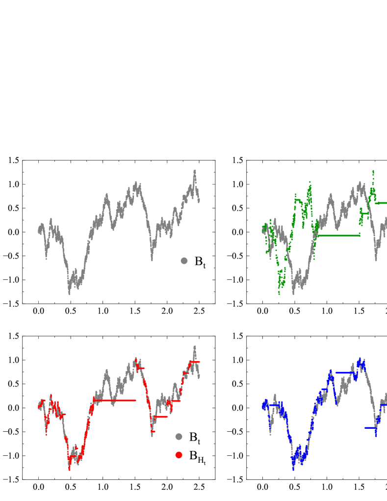
For illustrative purposes, we look at the Brownian motion and time-change it with the tempered -stable inverse subordinator and its undershooting and overshooting processes; see Figure 2.
Figure 2. Time-changed Brownian motion. The Brownian motion shown on the top-left is time-changed with the tempered -stable inverse subordinator of the previous figure, i.e. Figure 1 (A) right-hand side, and shown in the top-right. The bottom figures show the same Brownian motion time-changed with the undershooting and overshooting processes (left and right side, respectively) of Figure 1 (A) and (B) on the right-hand side, respectively.
4.1. Monte Carlo approximations
In this section, which draws inspiration from the recent research [53], we want to pose our attention to the Monte Carlo approximation of functionals of the process ,
(4.6)
where , is a -dimensional Feller process, and, as before, stands for the inverse subordinator or the undershoot process , or the overshoot process , of a given subordinator , where no distinction between the three is needed.
It is noteworthy that our study builds upon and generalizes the findings of previous research in this field in the following aspects. Any inverse subordinator and undershooting processes are considered, as well as any overshooting process that satisfies (4.33). We consider any -dimensional Feller process instead of -dimensional isotropic stable process. The availability of exact sample paths of inverse, undershoot, and overshoot processes allows us to consider general functionals of the time-changed process instead of only the single time position.
Note that the distribution of under does not depend on and so for this distribution we use the symbol
(4.7)
whenever there is no need to distinguish between the inverse subordinator, undershooting, or overshooting.
In particular, if is the inverse subordinator, then the term in (4.6) for gives the stochastic representation of the unique solution (in a suitable sense) to the general Cauchy problem
(4.8)
(4.9)
Here is the infinitesimal generator of the Feller process , and the operator is a non-local in time operator which can be defined in different ways. Still, the most popular is as a fractional-type derivative (see e.g. [18; 50]):
(4.10)
However, different approaches are also possible, see e.g. [51].
If instead is the undershoot , then (4.6) for is the stochastic representation of the unique solution to
(4.11)
(4.12)
where the non-local operator is non-local in time and space and given by
The Monte Carlo approximation of (4.6) that we consider here is the random variable
(4.13)
where and are independent and identically distributed samples of the processes and , respectively.
It is clear that by the strong law of large numbers -a.s. as , if is well-defined.
For this estimator we study the central limit theorem and Berry-Esseen theorem. First, we provide general conditions for which these theorems can be obtained and after that we show that these conditions are satisfied, for example, by all the isotropic Lévy processes. In our theorems we will control the behaviour of at the infinity. In particular, we will adopt the notation
(4.14)
Theorem 4.3.
Let be locally bounded and suppose that there exists such that . If , suppose additionally that
If, furthermore, (4.15) is replaced by the condition
(4.17)
for some , then for all such and all , it holds that
(4.18)
where .
Proof.
For the first result, it is enough to check that the second moment of is finite and to apply the central limit theorem. If , the result is trivial so we proceed with calculations for . Note that for any we have
(4.19)
By the assumption on the growth of and by suitably choosing , we obtain
(4.20)
for some . We deal with the term in (4.20) only since the first one is finite by the local boundedness of .
Note that is decreasing in so for any we get
Further, by a simple conditioning argument we have
Thus, the second moment is finite and we can apply the central limit theorem to finish the proof of the first claim.
For the second claim, by the very same argument, it is possible to see that
(4.23)
so the claim follows by an application of the Berry-Esseen Theorem, see e.g. [68, page 355].
∎
Now we show that a class of processes satisfies the condition of the previous theorem.
4.1.1. Isotropic Lévy processes
In this subsection we assume that the process , , is an isotropic Lévy process. This means that the process is characterized by the Lévy-Khintchine characteristic exponent
(4.24)
for a function with the representation
Here , the measure is the Lévy measure, i.e. it is such that
(4.25)
and the symbol stands for the law of under . A Lévy process is isotropic since both the Lévy measure and the law are isotropic measures, i.e. they are invariant upon linear isometries on .
Stable distributions (with the zero skewness parameter) exemplify isotropic Lévy measures, and the Cauchy distribution is a special case of these distributions.
In the following, Pruitt’s function for our -dimensional isotropic Lévy process will be relevant, i.e. the function
This function is strictly positive and decreasing (see more on[14; 72]) and in particular by [14, Remark 1] we have that
(4.26)
Then we have the following result.
Proposition 4.4.
Let be the inverse or the undershooting of a subordinator.
If the process is an isotropic Lévy process in , then the condition (4.15) is satisfied for any and for any such that
(4.27)
while the condition (4.17) is satisfied for any and for any such that
(4.28)
Proof.
Using (4.26) we get, for any constant which is enough larger than , that
(4.29)
The second integral in (4.29) is finite since the expectation of an inverse subordinator always exists and equals to the renewal measure, see [12, Section 1.3], while the undershooting is a.s. bounded by . For the first integral note that
(4.30)
(4.31)
The integral in (4.30) is convergent by (4.27) so we are left to check the integral in (4.31). We have that
(4.32)
where the integrals in (4.32) are finite by the definition of Lévy measure and the assumption (4.27). The second statement follows by using the very same argument and the assumption (4.28).
∎
Proposition 4.5.
Let be the overshooting of a subordinator whose Lévy measure satisfies
(4.33)
If the process is an isotropic Lévy process in then the condition (4.15) is satisfied for any and for any such that
(4.34)
while the condition (4.17) is satisfied for any and for any such that
(4.35)
Proof.
The proof is conducted in the same way as the proof of Proposition 4.4 up to the equation (4.29). Then, in order to check that the overshooting has finite expectation we use [12, Proposition 2 in Chapter III] to see that the distribution of on is given by , where is the potential measure of the subordinator. Here we do not have to integrate at zero because we assume which implies that . Thus
(4.36)
(4.37)
To finish the proof, we change the variables in the inner integral of (4.37) to get
Here, the finiteness of the integral follows from the fact that is a Lévy measure, and from the assumption (4.33). Further, is the renewal function of the subordinator and as such it is finite, see [12, Chapter III]. Further, it holds that which follows by [12, Proposition 2 in Chapter III].
∎
Remark 4.6.
For example, suppose that , , is a one-dimensional isotropic stable process with exponent , . Then the conditions (4.27) and (4.28) are satisfied, respectively, by and . In other words, in the case of the isotropic stable process , we can indeed consider exploding functionals in Theorem 4.3.
Remark 4.7.
Theorem 4.3, allows us to state the following convergence in distribution
Eq. (4.20) and (4.22) provide an upper bound to . The asymptotic confidence interval is
(4.38)
where is -quantile of the standard normal distribution. Moreover, it is clear that for a desired tolerance error , has to satisfy
(4.39)
The calculation of such estimator has complexity , that is, , or and , respectively.
5. Approximate simulation of time-changed processes
In this section, we deviate from the preceding one by considering Feller processes for which exact sampling is not necessarily available. In particular, we focus on -dimensional diffusions of the form
(5.1)
where is the (possible random) initial condition and is an -dimensional Wiener process, whose components are independent Wiener processes. The functions, and are measurable functions so the equations (5.1) is, component by component,
(5.2)
It is well-known that the stochastic differential equation (5.1) has a unique (strong) solution whenever has a finite second moment and the coefficients satisfy the standard Lipschitz conditions, see [47; 71].
For a suitably time-changed diffusion process, , stochastic calculus was developed in [48; 36; 45; 43].
This is deeply connected with (5.1) by the so-called duality principle [48, Theorem 4.2], which states that if is the unique solution to (5.1), then the time-changed process is the unique solution to
(5.3)
The theory of equations having the form (5.3) is valid for suitable time-changes that are in the so-called synchronization, see [48] for details. In our case the connection with the theory of (5.3) is clear in the case , i.e. when the time-change is the inverse of a subordinator (independent from the diffusion). For example, the case when the time-change is the undershooting is not covered by the theory in [48] since is a left-continuous process (and so is ). In view of the independence between the diffusion and the random time process, the sampling of two components can be done separately as explained in the previous section. However sometimes it happens that the diffusion cannot be sampled exactly. In this case several approximation methods exist. The more classical ones are the Euler-Maruyama method, its semi-implicit version or the Milstein schemes, but many others exist (see, e.g., [22] for a scheme in case the SDE has a distributional drift). With a scheme at hand one can approximate the diffusion part to obtain an approximation of the time-changed process. Hence, in our context, the representation (5.3) is not needed to sample the time-changed process nor to evaluate the approximation error.
We focus on evaluating the approximation error when the diffusion process is sampled using the Euler-Maruyama method. In the literature, the approximation error results are known also for different schemes. For example, the semi-implicit version of the Euler-Maruyama method has been studied in [23], but only in the case when the time-change is performed with an independent inverse subordinator, although for very general drift coefficients. This method, however, besides the error induced by the approximation of the diffusion includes also the error induced by the approximation method for the paths of the inverse subordinator. Further, the authors of [23] evaluate the strong convergence order (in the sense of ) which is of the same order as we get in Theorem 5.3, cf. Theorems 3.1 and 3.2 in [23]. Also, the Milstein method, which improves the Euler-Maruyama scheme but requires stronger assumptions on the diffusion coefficients, has been studied for time-changed diffusion via inverse subordinator, see [44] and also [58] where a similar equation is considered. In these papers, the authors used an approximation method for the trajectories of inverse subordinators, too. Clearly, approximation of the paths of the random time introduces a further error that with our method is avoided. For a more elaborate statement, see Remark 5.2 below.
Without loss of generality, from now on we assume that . The Euler-Maruyama approximation of the solution to SDE (5.1) with the time-steps , where is given by [47, Section 10.2]:
(5.4)
where , and , and denotes the maximum time step . We will denote the linear interpolation of , , as , i.e. component by component we have
(5.5)
In essence, the Euler-Maruyama approximation depends on all the grid , and not only on the maximum step size , but our results will be uniform for all grids with the prescribed maximum step size , so we proceed with this slightly abbreviated notation.
Usually, for ordinary differential equations, one evaluates the error as . Accordingly, for a stochastic differential equation, the classical approach is to evaluate the strong error as which is the straightforward generalization of the deterministic case, see [47, Section 9.6]. Instead, we adopt here the stronger criterion that bounds the strong error as follows
(5.6)
In [45, Propositions 3.1 and 3.2] it is proved that, when and satisfy suitable assumptions, the approximation (5.5) converges with the strong order of (and with the weak order of 1) to the exact solution. The following lemma provides the explicit constants involved in the strong error of the approximation of the solution to (5.1) by the Euler-Maruyama method. Since the proof is an adaptation of the method from [45], we postpone it to the Appendix. Before we present the exlicit constants, we bring the assumptions on the SDE (5.1) that will be used throughout the section.
(A).
The initial condition of the SDE (5.1) satisfies , while the drift and the diffusion coefficients satisfy
(5.7)
(5.8)
(5.9)
for all , , , where denotes the Euclidean norms in appropriate dimensions, and the constants and do not depend on .
Lemma 5.1.
Let (A) hold and suppose that the Euler-Maruyama approximation is defined using an arbitrary grid with the maximum step size .
Then there exist such that the strong error of the Euler-Maruyama approximation is finite and satisfies
(5.10)
where
and
Furthermore, by using [45, Proposition 3.2] it is also possible to evaluate the weak error, i.e.
(5.11)
for a suitable constant . However, this estimates requires several conditions on the growth of the coefficients of the SDE and of the solution to the associated transition density.
Remark 5.2.
In the following theorems, we provide the strong errors with explicit constants (which come from Lemma 5.1). These results not only extend, but also enhance the results available in the existing literature for two reasons. First, there is an increased flexibility in options concerning a time-change. Second, Algorithms 1 and 2 return exact paths, whereas existing literature approximates both the diffusion and the time-change paths, thereby inducing two errors (see the proof of Theorem 3.1 in [45]):
(5.12)
The first right-hand side term concerns the approximation of the inverse subordinator path, while the second term concerns the approximation of a diffusion process. Obviously, by using the exact sampling method for the inverse subordinator that we derived in Section 3, in our approximations there is no need for a division as in (5.12), provided that one consider an exact simulation whose output can be controlled with machine precision under the Lévy-Prokhorov metric, as explained in Section 2.
Here is the algorithm that we use to approximate the process .
Let be where is the solution to (5.3) satisfying (A). For , let , where , be the approximation of given in Algorithm 4. Then, for being the undershooting, the strong error is finite and satisfies
(5.13)
Additionally, for being the inverse of a subordinator with the Laplace exponent , the strong error is finite and satisfies
(5.14)
where is any constant such that .
Proof.
By Lemma 5.1 and the independence between the and , we observe that
(5.15)
(5.16)
Now, when is the undershooting, we use that to obtain the claim.
If, on the other hand, is the inverse of a subordinator, by Lemma A.3 for any such that it holds
(5.17)
which gives the claim.
∎
The time-change with the overshooting requires a separate statement since the strong error is finite under some more restrictive assumptions. Recall that the potential measure of the subordinator is defined as , . Now we have the statement for the strong error of the time-changed process with the overshooting.
Theorem 5.4.
Let where is the solution to (5.3) satisfying (A). For , let , where , be the approximation of as in Algorithm 4. If , where
(5.18)
then the strong error is finite and it holds that
(5.19)
Proof.
The proof can be conducted similarly to the proof of Theorem 5.3. We have
(5.20)
(5.21)
We are left to bound . Recall that on has the distribution and that , see [12] and the comments in the proof of Proposition 4.5. We have
(5.22)
By Fubini’s theorem and by the change of variables in the second integral we get
(5.23)
(5.24)
To bound the integral in (5.24), we distinguish two cases: and . If , then for the integral in (5.24) we have
(5.25)
Thus, by collecting the bounds (5.24) and (5.25) we obtain
(5.26)
For , we have a similar calculation where we separate the integral in (5.24) in the following way:
(5.27)
Thus, by collecting the bounds (5.24) and (5.27) we get
(5.28)
By combining bounds in (5.26) and (5.28), we obtain the claim of the proof.
∎
Remark 5.5.
The Algorithm 4 can be conducted with any grid, not just with the grid of equidistant number of points , as long as the maximum step size is bounded by , and the corresponding bounds on the strong error of approximation of , proved in Theorems 5.3 and 5.4 remain the same. This holds since the strong error of Euler-Maruyama is uniformly bounded among all grids with the maximum step , proved in Lemma 5.1.
Moreover, by using this uniformness, it is even allowed to add the sampled points to the grid . The maximum step size of the new grid is again , and the same bounds from Theorems 5.3 and 5.4 hold by using the so-called freezing lemma.
Proposition 5.6.
Assume (A). For a desired tolerance on the strong error of the approximation of by on , the complexity is
(5.29)
if , and
(5.30)
if or (with the additional assumption defined in (5.18) in this case), where was defined in Proposition 3.5.
The random variables in (5.29) and (5.30) have finite moments of all order and their expectation can be bounded by using Proposition 3.5.
Proof.
The Algorithm 4 first samples the time-change , , which has the cost of in the case , and in the case or , see Proposition 4.1.
Then comes the sampling of the Euler-Maruyama scheme. If is the desired error tolerance on the paths of , then the time step has to satisfy
(5.31)
see Theorem 5.3 and (5.16), and Theorem 5.4 and (5.21).
It is clear that by choosing small enough, this can be achieved for any . For such that the equality in (5.31) holds, the number of grid points for the Euler-Maruyama scheme is , and they all have the cost of one since they only consist of elementary operations. To calculate the values , we need to calculate additional interpolations, which have the cost of one. By summing up those costs, and by noting that
the statement on the complexity follows.
Since , in all the cases, the claim for finite moments of all order easily follows.
∎
5.1. Monte Carlo approximations of time-changed diffusion processes
We consider now the Monte Carlo estimator for where is a time-changed diffusion process as above and is a suitable locally bounded functional. The estimator is given by
(5.32)
and is the counterpart of (4.13) in the case when an exact simulation of the Markov process is not at hand. Here we evaluate the error in the approximation.
Theorem 5.7.
Assume (A) and let be such that , for a positive constant and , . Then
(5.33)
where
(5.34)
where .
Furthermore, the expectation in (5.34) can be bounded as in Theorems 5.3 and 5.4, where for the case we additionally assume defined in (5.18).
Proof.
First note that
(5.35)
Indeed, by argumentation as in Theorem 4.3 for (4.20) (since by the Lipschitz assumption on ) we get
(5.36)
(5.37)
(5.38)
where in the last line we used Lemma A.1 and the fact that is non-decreasing. This proves the finiteness of the first two moments, where for the case we must note that so by the assumption .
Note that
(5.39)
Note that, under assumption , the second term on the right-hand side can be bounded by the strong error as in Theorem 5.3, as follows
(5.40)
Therefore, by using (5.6) and Theorem 5.3 or Theorem 5.4, the second right term in (5.39) is bounded by .
Further, for we have
(5.41)
(5.42)
where we used Lemma A.1 and Lemma 5.1, and that .
Hence, by the same reasoning as in the beginning of the proof, we obtain
(5.43)
(5.44)
By collecting these two bounds for terms in (5.39), we get the claim.
∎
Proposition 5.8.
Assume (A) and fix the tolerance error . For the computation of the estimator (5.32) with -error smaller than , the complexity is bounded by
(5.45)
if , and
(5.46)
if or (with the additional assumption in this case, see (5.18)).
The constants and come from Theorem 5.7, and from Lemma 5.1, while comes from Section 2.1.
The random variables in (5.45) and (5.46) have finite moments of all order, and their expectation can be bounded by using Proposition 3.5. The exponential moments of are bounded in Theorems 5.3 and 5.4.
Proof.
Fix . Choose and such that and . In this way the bound (5.33) is smaller than . Therefore, must be bigger than , and must be smaller than
(5.47)
Now the complexity of the estimator (5.32) is given as
multiplied by the Euler-Maruyama complexity which is given in Proposition 5.6 by using the time step .
The aforementioned substantiates the proposition claim.
∎
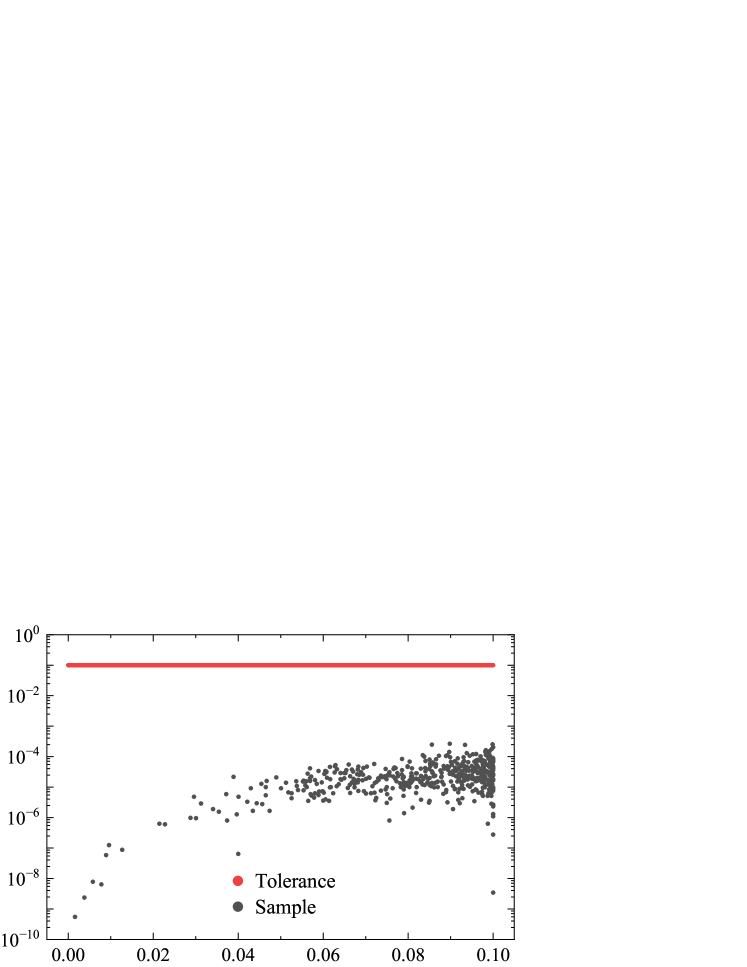
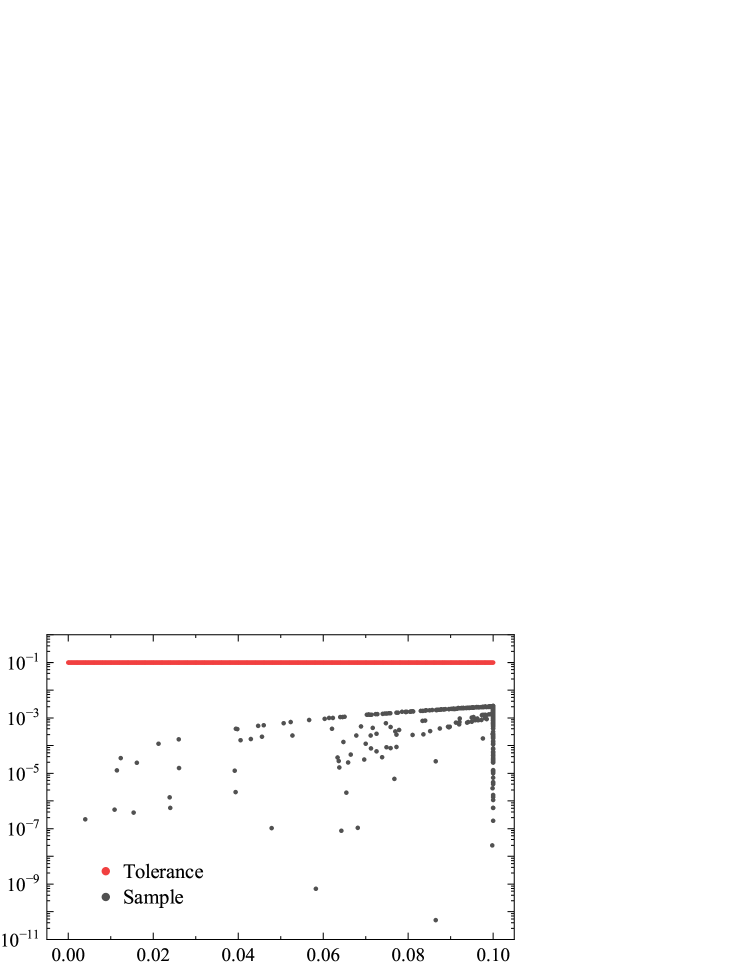
5.1.1. Numerical examples
In the following examples we consider diffusions for which the explicit solution is known, approximate it using Algorithm 4, and compute the error
(5.48)
for 500 independent trajectories. The results are shown in Figure 3.
Example 5.9.
We consider the time-changed (with inverse subordinator) Ornstein-Uhlenbeck process,
where , and , , which is a subdiffusion and a special case of a fractional Pearson diffusion. For further details about these subdiffusions see [3; 57]. In particular, let be the inverse of an -stable subordinator, , , , , and , . Fix the tolerance error and use formula (5.31) to get .
Figure 3(a) shows independent samples of the error (5.48) for the desired tolerance error.
These agree with the findings of Theorem 5.3.
Example 5.10.
The process , , with solves the stochastic differential equation
see [47, Chapter 4.4] for details. We time-change this diffusion with the undershooting process of an -stable subordinator, , in , and consider and . Further, we may choose . Now we fix the tolerance error and compute that by using (5.31). By executing Algorithm 4, the error (5.48) is calculated. The results are shown in Figure 3(b), which corroborate the findings of Theorem 5.3.
(a)Ornstein-Uhlenbeck, time-changed with the inverse of an -stable subordinator.
(b)Diffusion, time-changed with the undershooting process of an -stable inverse subordinator.
Figure 3. 500 independent error (5.48) samples for two different diffusions, with a desired tolerance error . Each point represents the maximum error obtained by a sample and its corresponding time point at which the error occurred.
5.1.2. The limit distribution
Now we study the limit distribution of the Monte Carlo estimator defined in (5.32) when the time step and jointly, i.e., we put as .
Denote
(5.49)
where are independent samples of . Define
(5.50)
First we need to verify that for a suitable choice of the random variables in (5.50) form a null array.
According to [46, p. 88], a null array is a triangular array of random variables or vectors , , , such that the are independent for each and satisfy , in probability, as , uniformly in .
Lemma 5.11.
Assume (A) and , for and .
Set , with , and if , additionally assume defined in (5.18). Then the random variables (5.50) form a null array.
Proof.
Using Markov, triangular and Cauchy-Schwartz inequalities, we have
(5.51)
Note that is bounded by using (5.44) while can be bounded as in (5.40). Therefore,
The proof of our theorem consists of proving conditions (1), (2), and (3) of Theorem 5.13 for defined in (5.50).
Proof of condition (1).
Note that
(5.54)
Hence
(5.55)
In the same spirit as [53, Equation 3.41], the second term on the right-hand side goes to zero as :
(5.56)
Using the Markov inequality, (5.40), and (5.6) and Theorems 5.3 and 5.4, we have
(5.57)
which tends to as .
Proof of condition (2).
In the same fashion as above we have that
(5.58)
as . Therefore it is enough to check that
(5.59)
which is, then, equivalent to proving condition (2).
For a random variable , we denote . Then
(5.60)
(5.61)
(5.62)
Theorem 5.7 implies that the first term of (5.62) goes to zero as .
The second term in (5.62) goes to zero by the dominated convergence theorem, since by the calculations from the beginning of the proof of Theorem 5.7. Hence,
(5.63)
Similarly, denote . Then, by repeating the very same steps as above we have that
(5.64)
By combining (5.63) and (5.64), condition (2) holds with .
Proof of condition (3). We have that
(5.65)
The following lines prove that the second term on the right-hand side of the above equation goes to zero as .
(5.66)
Note that so
(5.67)
Similarly,
(5.68)
Substituting equations (5.67) and (5.68) into (5.1.2) and using equations (5.63), (5.64), and (5.58), shows that (5.1.2) goes to zero as . Indeed, (5.67) also tends to zero by dominated convergence theorem, using (5.35).
Now, we will prove
(5.69)
Use the Cauchy-Schwarz inequality to note that
(5.70)
Since (as proved in (5.35)) and (with the help of (5.58)) , and furthermore we know that have a uniform upper bound for all by equation (5.42). Hence have a uniform upper bound for all . Hence
The choice of , , is not unique in the sense that the proof of the previous claim holds even if as which can be seen by inspecting the proof.
Remark 5.15.
In the classical case of Monte Carlo approximations for the Euler-Maruyama scheme, one chooses and then so that , i.e. . In this case, the bound of the error of the approximations, given in Theorem 5.7, is
(5.74)
If the tolerance for the error of the approximations is , then we can choose so that . In this case, the complexity (obtained by repeating the reasoning as in Proposition 5.8) is bounded by
if , and
if or (with the additional assumption in this case, see (5.18)).
The explicit expressions for constants in the lines above can be found in Theorem 5.7 and Lemma 5.1, while comes from Section 2.1.
, , , which together with the Gronwall’s inequality (see [47, Lemma 4.5.1]), yields
Note that for all , , so we get
∎
Remark A.2.
For time-independent coefficients, the constant becomes
Lemma A.3.
Let be a subordinator given by (3.1), and its inverse. Then, for any , and for any such that it holds that
Proof.
The proof of this claim follows by repeating exactly the same steps as in [33, Lemma A.1].
∎
Acknowledgments
The authors acknowledge financial support under the National Recovery and Resilience Plan (NRRP), Mission 4, Component 2, Investment 1.1, Call for tender No. 104 published on 2.2.2022 by the Italian Ministry of University and Research (MUR), funded by the European Union – NextGenerationEU– Project Title “Non–Markovian Dynamics and Non-local Equations” – 202277N5H9 - CUP: D53D23005670006 - Grant Assignment Decree No. 973 adopted on June 30, 2023, by the Italian Ministry of University and Research (MUR).
The authors would like to thank the Isaac Newton Institute for Mathematical Sciences, Cambridge, for support and hospitality during the programme Stochastic systems for anomalous diffusion, where work on this paper was undertaken. This work was supported by EPSRC grant EP/Z000580/1.
The authors would like to thank Prof. Aleksandar Mijatović for fruitful discussions on the
topic that improved a previous version of this manuscript.
References
[1]
D. Applebaum.
Lévy processes and stochastic calculus.
Cambridge University Press, New York, second edition, 2009.
[2]
G. B. Arous, M. Cabezas, J. Černý, and R. Royfman.
Randomly trapped random walks.
The Annals of Probability, 43(5):2405–2457, 2015.
[3]
G. Ascione, N. Leonenko, and E. Pirozzi.
Time-Non-Local Pearson diffusions.
Journal of Statistical Physics, 183(48), 2021.
[4]
G. Ascione, E. Pirozzi, and B. Toaldo.
On the exit time from open sets of some semi-Markov processes.
The Annals of Applied Probability, 30(3):1130–1163, 2020.
[5]
G. Ascione, M. Savov, and B. Toaldo.
Regularity and asymptotics of densities of inverse subordinators.
Transactions of the London Mathematical Society, 11(1):e70004,
2024.
[6]
G. Ascione, E. Scalas, B. Toaldo, and L. Torricelli.
Time-changed Markov processes and coupled non-local equations.
arXiv:2412.14956, 2024.
[7]
S. Asmussen and P. W. Glynn.
Stochastic simulation: Algorithms and analysis.
Springer, 2007.
[8]
B. Baeumer and M. M. Meerschaert.
Stochastic solutions for fractional Cauchy problems.
Fractional Calculus and Applied Analysis, 4:481–800, 2001.
[9]
B. Baeumer, M. M. Meerschaert, and J. Mortensen.
Space-time fractional derivative operators.
Proceedings of the American Mathematical Society,
133(8):2273–2282, 2005.
[10]
E. Barkai, Y. Garini, and R. Metzler.
Strange kinetics of single molecules in living cells.
Physics Today, 65(8):29–35, 2012.
[11]
E. Barkai, R. Metzler, and J. Klafter.
From continuous time random walks to the fractional Fokker-Planck
equation.
Physiscal Review E, 61:132–138, 2000.
[12]
J. Bertoin.
Lévy processes.
Cambridge University Press, Cambridge, 1996.
[14]
K. Bogdan, T. Grzywny, and M. Ryznar.
Barriers, exit time and survival probability for unimodal Lévy
processes.
Probability Theory and Related Fields, 162:155–198, 2015.
[15]
B. Böttcher, R. Schilling, and J. Wang.
Lévy Matters III. Lévy-Type Processes: Construction,
Approximation and Sample Path Properties.
Springer, 2013.
[16]
B. Casella and G. O. Roberts.
Exact simulation of jump-diffusion processes with Monte Carlo
applications.
Methodology and Computing in Applied Probability, 13:449–473,
2011.
[17]
E. Çinlar.
Markov additive processes. I.
Zeitschrift für Wahrscheinlichkeitstheorie und Verwandte
Gebiete, 24:85–93, 1972.
[18]
Z.-Q. Chen.
Time fractional equations and probabilistic representation.
Chaos, Solitons and Fractals, 102:168–174, 2017.
[19]
Z. Chi.
On exact sampling of the first passage event of a Lévy process
with infinite Lévy measure and bounded variation.
Stochastic Processes and their Applications, 26(4):1124–1144,
2016.
[20]
T. H. Cormen, C. E. Leiserson, R. L. Rivest, and C. Stein.
Introduction to Algorithms.
The MIT Press, fourth edition, 2022.
[21]
A. Dassios, J. W. Lim, and Y. Qu.
Exact simulation of a truncated Lévy subordinator.
ACM Transactions on Modeling and Computer Simulation, 30(3):17,
2020.
[22]
T. De Angelis, M. Germain, and E. Issoglio.
A numerical scheme for stochastic differential equations with
distributional drift.
Stochastic Process. Appl., 154:55–90, 2022.
[23]
C.-S. Deng and W. Liu.
Semi-implicit Euler-Maruyama method for non-linear time-changed
stochastic differential equations.
BIT Numerical Mathematics, 60:1133–1151, 2020.
[24]
A. Di Gregorio and F. Iafrate.
Path dynamics of time-changed Lévy processes: A martingale
approach.
Journal of Theoretical Probability, 37:3246–3280, 2024.
[25]
R. M. Dudley.
Distances of probability measures and random variables.
The Annals of Mathematical Statistics, 39(5):1563–1572, 1968.
[26]
F. Falcini, R. Garra, and V. Voller.
Modeling anomalous heat diffusion: Comparing fractional derivative
and non-linear diffusivity treatments.
International Journal of Thermal Sciences, 137:584–588, 2019.
[27]
S. Fedotov.
Non-Markovian random walks and nonlinear reactions: Subdiffusion
and propagating fronts.
Physical Review E, 81:011117, 2010.
[28]
S. Fedotov, N. Korabel, T. A. Waigh, D. Han, and V. J. Allan.
Memory effects and Lévy walk dynamics in intracellular transport
of cargoes.
Physical Review E, 98:042136, 2018.
[29]
S. Fedotov and V. Méndez.
Non-Markovian model for transport and reactions of particles in
spiny dendrites.
Physical Review Letters, 101:218102, 2008.
[30]
D. Fulger, E. Scalas, and G. Germano.
Monte Carlo simulation of uncoupled continuous-time random walks
yielding a stochastic solution of the space-time fractional diffusion
equation.
Physical Review E, 77(2):021122, 2008.
[31]
M. T. Giraudo, L. Sacerdote, and C. Zucca.
A Monte Carlo method for the simulation of first passage times of
diffusion processes.
Methodology and Computing in Applied Probability, 3:215–231,
2001.
[32]
J. I. González Cázares, F. Lin, and A. Mijatović.
Fast exact simulation of the first-passage event of a subordinator.
arXiv:2306.06927, 2024.
[33]
J. I. González Cázares, F. Lin, and A. Mijatović.
Fast exact simulation of the first passage of a tempered stable
subordinator across a non-increasing function.
Stochastic Systems, (in press), 2024.
[34]
R. Gorenflo, F. Mainardi, D. Moretti, G. Pagnini, and P. Paradisi.
Discrete random walk models for space–time fractional diffusion.
Chemical Physics, 284(1):521–541, 2002.
[35]
R. Gorenflo, F. Mainardi, and A. Vivoli.
Continuos-time random walk and parametric subordination in fractional
diffusion.
Chaos, Solitons and Fractals, 34(1):87–103, 2007.
[36]
M. Hahn, K. Kobayashi, and S. Umarov.
SDEs driven by a time-changed Lévy process and their associated
time-fractional order pseudo-differential equations.
Journal of Theoretical Probability, 25:262–279, 2012.
[37]
M. Hairer, G. Iyer, L. Koralov, A. Novikov, and Z. Pajor-Gyulai.
A fractional kinetic process describing the intermediate time
behaviour of cellular flows.
The Annals of Probability, 46(2):897–955, 2018.
[38]
M. Hairer, L. Koralov, and Z. Pajor-Gyulai.
From averaging to homogenization in cellular flows - an exact
description of the transition.
Annales de L’institut Henri Poincaré - Probabilités et
Statistiques, 52(4):1592–1613, 2016.
[39]
B. Harlamov.
Continuous semi-Markov processes.
John Wiley & Sons, 2013.
[40]
M. E. Hernández-Hernández, V. N. Kolokoltsov, and L. Toniazzi.
Generalised fractional evolution equations of Caputo type.
Chaos, Solitons and Fractals, 102:184–196, 2017.
[41]
S. Herrmann and C. Zucca.
Exact simulation of the first-passage time of diffusions.
Journal of Scientific Computing, 9(3):1477–1504, 2019.
[42]
A. Jacquier and L. Torricelli.
Anomalous diffusions in option prices: connecting trade duration and
the volatility term structure.
SIAM Journal on Financial Mathematics, 11(4):1137–1167, 2020.
[43]
S. Jin and K. Kobayashi.
Strong approximation of stochastic differential equations driven by a
time-changed Brownian motion with time-space-dependent coefficients.
Journal of Mathematical Annalysis and Applications,
479(2):619–636, 2019.
[44]
S. Jin and K. Kobayashi.
Strong approximation of time-changed stochastic differential
equations involving drifts with random and non-random integrators.
BIT Numerical Mathematics, 61:829–857, 2021.
[45]
E. Jum and K. Kobayashi.
A strong and weak approximation scheme for stochastic differential
equations driven by a time-changed Brownian motion.
Probability and Mathematical Statistics, 36(2):201–220, 2016.
[46]
O. Kallenberg.
Foundations of Modern Probability.
Springer, second edition, 2002.
[47]
P. E. Kloeden and E. Platen.
Numerical solution of stochastic differential equations.
Springer, 1992.
[48]
K. Kobayashi.
Stochastic calculus for a time-changed semimartingale and the
associated stochastic differential equations.
Journal of Theoretical Probability, 24:789–820, 2011.
[49]
A. N. Kochubei.
Distributed order calculus and equations of ultraslow diffusion.
Journal of Mathematical Analysis and Applications,
340(1):252–281, 2008.
[50]
A. N. Kochubei.
General fractional calculus, evolution equations and renewal
processes.
Integral Equations and Operator Theory, 71:583–600, 2011.
[51]
V. N. Kolokoltsov.
On fully mixed and multidimensional extensions of the Caputo and
Riemann-Liouville derivatives, related Markov process and fractional
differential equations.
Fractional Calculus and Applied Analysis, 18(4):1039–1073,
2015.
[52]
V. N. Kolokoltsov.
The rates of convergence for functional limit theorems with stable
subordinators and for CTRW approximations to fractional evolutions.
Fractal and Fractional, 7(4):335, 2023.
[53]
V. N. Kolokoltsov, F. Ling, and A. Mijatović.
Monte Carlo estimation of the solution of fractional partial
differential equations.
Fractional Calculus and Applied Analysis, 24(1):278–306, 2021.
[54]
R. A. Kronmal and A. V. Peterson.
A variant of the acceptance-rejection method for computer generation
of random variables.
Journal of the American Statistical Association,
76(374):446–451, 1981.
[55]
R. A. Kronmal and A. V. Peterson.
An acceptance-complement analogue of the
mixture-plus-acceptance-rejection method for generating random variables.
ACM Transactions on Mathematical Software, 10(3):271–281,
1984.
[56]
N. Leonenko and I. Podlubny.
Monte Carlo method for fractional-order differentiation.
Fractional Calculus and Applied Analysis, 25:346–361, 2022.
[57]
N. N. Leonenko, M. M. Meerschaert, and A. Sikorskii.
Fractional Pearson diffusions.
Journal of Mathematical Analysis and Applications,
403(2):532–546, 2013.
[58]
W. Liu, R. Wu, and R. Zuo.
A Milstein-type method for highly non-linear non-autonomous
time-changed stochastic differential equations.
arXiv:2308.13999, 2023.
[59]
L. Lv and L. Wang.
Stochastic representation and Monte Carlo simulation for
multiterm time-fractional diffusion equation.
Advances in Mathematical Physics, 2020:1315426, 2020.
[60]
M. Magdziarz, A. Weron, and K. Weron.
Fractional Fokker-Planck dynamics: Stochastic representation and
computer simulation.
Physical Review E, 75(1), 2007.
[61]
M. M. Meerschaert and H.-P. Scheffler.
Limit theorems for continuous-time random walks with infinite mean
waiting times.
Journal of Applied Probability, 41(3):623–638, 2004.
[62]
M. M. Meerschaert and P. Straka.
Semi-Markov approach to continuous time random walk limit process.
The Annals of Probability, 42(4):1699–1726, 2014.
[63]
R. Metzler, E. Barkai, and J. Klafter.
Anomalous diffusion and relaxation close to thermal equilibrium: A
fractional Fokker-Planck equation approach.
Physical Review Letters, 82(18):3563–3567, 1999.
[64]
R. Metzler and J. Klafter.
The random walk’s guide to anomalous diffusion: a fractional dynamics
approach.
Physics Reports, 339(1):1–77, 2000.
[65]
A. Mijatović and V. Vysotsky.
Stability of overshoots of zero mean random walks.
Electron. J. Probab., 25:Paper No. 63, 22, 2020.
[66]
E. W. Montroll and G. H. Weiss.
Random walk on lattices II.
Journal of Mathematical Physics, 6(2):167–181, 1965.
[67]
A. Mura and G. Pagnini.
Characterizations and simulations of a class of stochastic processes
to model anomalous diffusion.
Journal of Physics A: Mathematical and Theoretical, 41, 2009.
[68]
R. O’Donnell.
Analysis of Boolean Functions.
Cambridge University Press, 2014.
[69]
A. Osȩkowski.
Sharp maximal inequalities for the martingale square bracket.
Stochastics, 82(6):589–605, 2010.
[70]
Y. Povstenko.
Fractional Thermoelasticity.
Springer International Publishing, 1st edition, 2015.
[71]
P. E. Protter.
Stochastic integration and differential equations.
Springer, 2nd edition, 2004.
[72]
W. E. Pruitt.
The growth of random walks and Lévy processes.
The Annals of Probability, 9(6):948–956, 1981.
[73]
D. Revuz and M. Yor.
Continuous martingales and Brownian motion.
Springer Science & Business Media, 3rd edition, 1999.
[74]
L. M. Ricciardi.
On the transformation of diffusion processes into the Wiener
process.
Journal of Mathematical Analysis and Applications,
54(1):185–199, 1976.
[75]
K.-I. Sato.
Lévy processes and infinitely divisible distributions.
Cambridge University Press, Cambridge, 1999.
[76]
M. Savov and B. Toaldo.
Semi-Markov processes, integro-differential equations and anomalous
diffusion-aggregation.
Annales de l’Institut Henri Poincaré, Probabilités et
Statistiques, 56(4):2640–2671, 2020.
[77]
H. Scher and M. Lax.
Stochastic transport in a disordered solid. I. Theory.
Physical Review B, 7(10):4491–4502, 1973.
[78]
H. Scher and M. Lax.
Stochastic transport in a disordered solid. II. Impurity
conduction.
Physical Review B, 7(10):4502–4519, 1973.
[79]
H. Scher and E. W. Montroll.
Anomalous transit-time dispersion in amophous solids.
Physical Review B, 12(6):2455–2477, 1975.
[80]
R. Schilling, R. Song, and Z. Vondraček.
Berstein functions Theory and applications.
De Gruyter, 2nd edition, 2012.
[81]
B. Toaldo.
Lévy mixing related to distributed order calculus, subordinators
and slow diffusions.
Journal of Mathematical Analysis and Applications,
430(2):1009–1036, 2015.
[82]
V. V. Uchaikin and V. V. Saenko.
Stochastic solution to partial differential equations of fractional
orders.
Sibirskii Zhurnal Vychislitel’noi Matematiki, 6(2):197–203,
2003.
[83]
G. M. Zaslavsky.
Fractional kinetic equation for Hamiltonian chaos.
Physica D: Nonlinear Phenomena, 76(1-3):110–122, 1994.
[84]
G. M. Zaslavsky.
Chaos, fractional kinetics, and anomalous transport.
Physics reports, 371(6):461–580, 2002.
[85]
G. M. Zaslavsky.
Hamiltonian Chaos and Fractional Dynamics.
Oxford University Press, 2005.
Ivan Biočić
Department of Mathematics, Faculty of Science, University of Zagreb, Zagreb, Croatia,
Department of Mathematics “Giuseppe Peano”, University of Turin, Turin, Italy,
Email: ivan.biocic@unito.it, ivan.biocic@math.hr
Daniel E. Cedeño-Girón
Department of Mathematics “Giuseppe Peano”, University of Turin, Turin, Italy,
Email: danieleduardo.cedenogiron@unito.it
Bruno Toaldo
Department of Mathematics “Giuseppe Peano”, University of Turin, Turin, Italy,