Extreme events in a random set of nonlinear elastic bending waves
Abstract
The processes that generate rogue waves on the sea surface remain a mystery. Despite their different natures, the nonlinear bending waves generated in a thin elastic plate share some similarities with waves on the surface of the sea. For instance, both involve four-wave interactions during energy exchange, but in bending waves, the number of waves is not conserved. Here, we present an experimental study to investigate extreme event statistics in random elastic bending waves forced by an electromagnetic shaker on a thin stainless steel plate. In our setup, the standard statistical criterion used to define extreme events, such as rogue waves on the sea surface, is insufficiently restrictive. We therefore apply a new criterion to determine the occurrence frequency of rare events, similar to those observed in wave tanks [5]. With this new criterion, we examine correlations between extreme events amplitude and wave slopes, energy, and periods, raising questions about the links between statistically rare events and rogue waves.
I Introduction
Among rare events that have dramatic consequences, one can mention the rogue waves on the ocean. Rogue waves are exceptionally large waves that occur in seas and oceans, for a given sea state. For a longtime they were only supported by seafarers’ testimonials and their consequences on ships and infrastructures damages, but there are now many direct field measurements evidencing the existence of this freak wave especially since the ‘New Year Wave’ recorded at the Draupner platform in the North Sea on the of January 1995[1, 2]. Field measurements are subject to many uncontrolled external factors hence they have been complemented by monitored experiments in order to capture the main ingredients involved in the generation of these huge events [3, 4, 5]. Among these many experiments, we highlight the recent experiment made in a large wave tank facility with a random narrow-banded white noise forcing [5]. We have used this work as reference for rogue wave statistics at water surface. The precise definition of rogue waves is controversial and may depend on who are concerned. One of the most accepted definition is the one based on the significant height of the waves, which is defined as the average height of the highest one-third of waves. Rogue waves are those whose height is at least twice this significant wave height . For surface waves, it reduces to a purely statistical threshold: rogue waves are events larger than eight times the standard deviation of the wave elevation[1, 2, 5].
It is clear that nonlinear interactions between waves play an important role although wave-stream coupling, wind stress and topography may also have important effects on the real sea state [1]. In the narrow band approximation, some nonlinear aspects are described by the Nonlinear Schrödinger Equation (NLSE) [6]. NLSE generates extreme events known as Peregrine solitons through a modulational instability. One can observe such structures in wave tank under very specific forcing. They are also observed in nonlinear optic and plasma physics that are well described by NLSE [3, 7, 8, 9]. However, such phenomenon might not include all the mechanisms of rogue wave formation in a random sea state with large spectra. Indeed, we know from the Weak or Wave Turbulence (WT) theory that the surface gravity wave generated at the water surface interact through a four waves process conserving the number of waves i.e., two mothers waves generate two daughters waves. This process implies a direct cascade of the wave energy and an inverse cascade of wave action [10]. The exact role of the nonlinear interactions and the precise effects of the inverse cascade on the occurrence of rogue waves remain unresolved.
To explore these effects, we study another set of nonlinear waves: the bending waves generated in a thin elastic plate. These waves, described by the Föppl–von Kármán equation [11], present some similitudes with the surface gravity waves in the framework of the WT. There are four interacting waves during energy exchange implying a direct cascade of energy predicted in [12]. Experiments differ from that prediction mainly due to dissipation [13, 14, 15]. In contrast to surface gravity waves, the number of waves and hence the wave action are not necessarily preserved. Therefore, there is no inverse cascade [12]. In that case, one can show that for scales larger than the forcing, there is no flux between scales in average implying an equipartition of the energy at these large scales [16]. This imposes a flat Power Density Spectrum (PDS) at low frequency, i.e. with the forcing frequency, for the speed of the surface displacement and a PDS in for waves amplitude (instead of for the surface gravity waves [10]). Another difference is the expected crest-trough symmetry in the bending wave problem that does not exist with surface where crests are sharper than trough [17].
We first shortly present the experimental device of the bending wave setup. Then the statistical characteristics of the local displacement and especially the fraction of extreme events is given for various forcing amplitudes and frequencies. In order to have relevant comparison with surface waves, we measure the correlation of these rare events amplitudes with different wave characteristics (periods, steepness, energy). The next part discusses the properties of rare events in a set of bending waves with those on gravity surface waves obtained in [5].
II Experimental Device and data processing
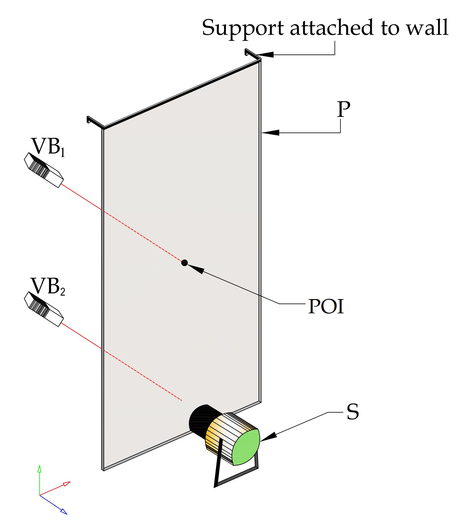
The setup, shown in figure 1, is similar to the one presented in [16]. A thin elastic plate ( mm3) is fasten to its support at the top and to an Electromagnetic (EM) shaker attached at 10 cm from the bottom. Others boundaries are free. In our device, the bending waves follow a quadratic dispersion relation such that with the wavenumber, the wavelength and where is proportional to the sound velocity in the bulk of the material ( being the Young modulus, the Poisson ratio, the specific mass of the stainless steel).The EM shaker is used to drive the plate to an out–of–equilibrium steady state by imposing a sinusoidal motion of various frequency and amplitude. The forcing frequency is such that the associated forcing wavelength, , is smaller than the plate size, , in order to capture the role of the wave at scales larger than the which are at equipartition of energy. Also, forcing bending waves at higher frequencies, such as 150 Hz and 250 Hz as in our study, offers a distinct advantage by providing significantly more statistics in a shorter time compared to surface wave experiments, which are typically limited to 2 Hz. A vibrometer is used to measure the plate displacement. Measurements are taken around the plate’s center, 20 cm from its boundaries, where the statistics are equivalent. In addition, we measure the velocity and the force at the energy injection point in order to quantify the level of turbulence by the energy input. For each forcing parameter, we performed a 10 hours measurement at a sampling rate of 4096 samples per second. The convergence of the extreme events statistics has been tested with a run of 62 hours.
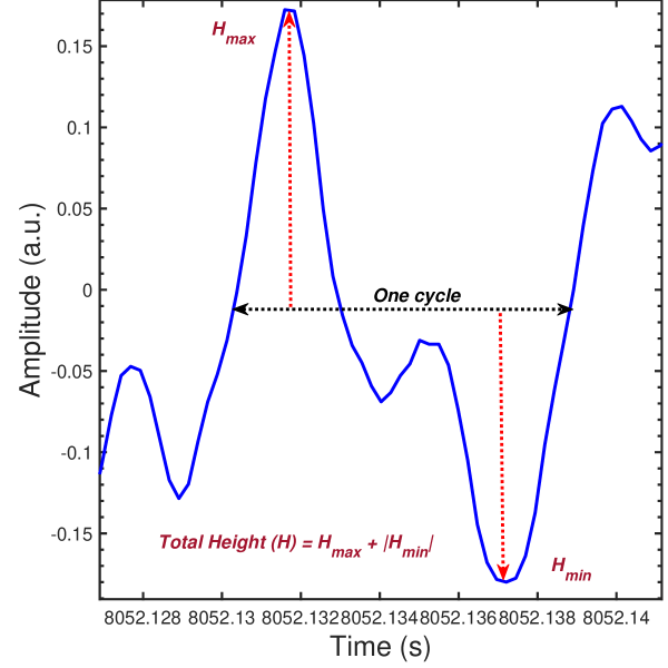
In order to mimic the rogue waves analysis, as in surface waves, we have to define a local wave period as the th interval between two zero crossing with the same slope sign of the transverse displacement . The wave crests, , and wave troughs, , are defined as the maximum and minimum values, respectively, during the local period (see the temporal trace in Figure 2). Then, the wave height, , is defined as the sum of and .
III experimental results
III.1 Statistics of the the bending waves amplitudes
III.1.1 Statistical properties of the displacement
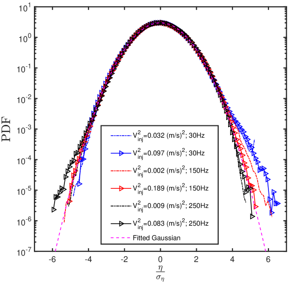
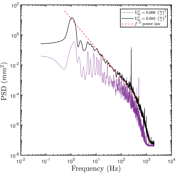
We first consider briefly the statistical properties of the transversal displacement directly measured by the vibrometer at one point near the plate center. In the nonlinear regime, the typical displacement fluctuations are depicted by their Probability Density Functions (PDF) figure 3 and their Power Density Spectrum (PDS) figure 4. In figure 3 fluctuations are nearly Gaussian in the nonlinear regime with sometime a small skewness. This skewness is very sensitive to any tiny misalignment of the plate with the vertical axis. The PDS are shown in figure 4 at low forcing and in the nonlinear regime with a forcing frequency . The low forcing spectrum exhibits the forcing frequency and the modes of the plates whereas the spectrum in the nonlinear regime is continuous above and below (up to a peak around nearly 1 Hz). The power law in exhibited for , is compatible with an equipartition of the energy with no energy flux in average in this range of frequency [16]. Note that this range will be significantly shrunken with the forcing frequency at Hz.
III.1.2 Statistical properties of the wave height
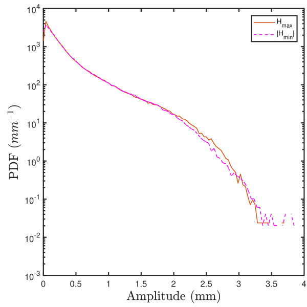
We focus now on the height, , as previously defined. The PDF of the height is shown on figure 5. Although the PDF of the transversal displacement is quite Gaussian, the shape of the PDF of the height is far from the Rayleigh distribution. Such Rayleigh distribution would describe the height of a random set of Gaussian and uncorrelated transversal displacement. It also accurately describes the height of gravity waves on water surfaces. The PDF’s of the bending waves height have fatter tail enhancing rare events in the nonlinear regime. In contrast to surface wave, these peculiar shapes are also found in the PDF of and which are symmetrical in figure 6, as expected by the symmetries of the setup (i.e. the fluctuations of and seem poorly affected by the small skewness observed for the displacement).
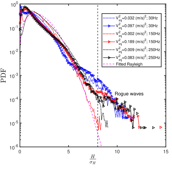
The traditional definition of rogue waves involves the significant wave height, . For surface sea waves, the height distribution follows a Rayleigh distribution, and corresponds to four times the standard deviation of the surface elevation, . Therefore, the most widely accepted definition of rogue waves is waves with a height such that .
In contrast, bending elastic waves exhibit a distribution with much fatter tails (see Figure 5). Consequently, using the criterion results in an event rate (about 1%) that is too high to classify such waves as rare. On the other hand, the stricter criterion is overly restrictive, as it corresponds to only one or two events occurring during 10 hours of experiments where such events are observed. This equates to a fraction of rare events less than in strongly forced cases, which is significantly lower than the rogue wave occurrence rates measured in wave tanks.
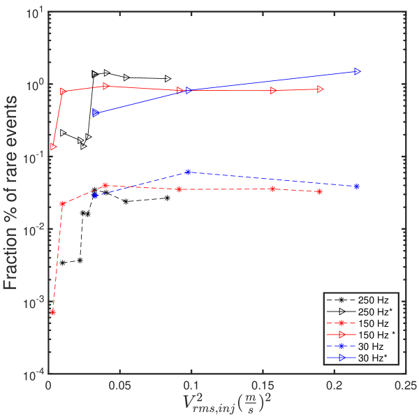
To recover the same fraction of rare events as in [5], we define them as where is now the standard deviation of the wave height. These are the events within the fat tails delimited by the black dasher line in figure 5. These fractions of rare events are shown figure 7 for various forcing. In the strongly forced fully nonlinear regime, it converges around a fraction of 0.02 to 0.06 % with no clear dependencies to the forcing frequency. It is about a few hundred events during the 10 hours measurements. In the next section, we look for the correlation of these rare events with others characteristics of the waves.
III.2 Correlation
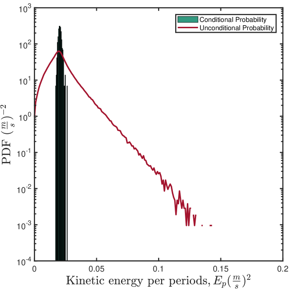
To capture the correlations between extreme events and other quantities characterizing the wave, like its kinetic energy per unit mass, its slope or its local periods, we are going to compare the PDF conditioned to the presence of an extreme event within the local period with the PDF without any condition. If the extreme events were uncorrelated to the considered quantities, PDF would remain unchanged. We focus on the driving in the strong nonlinear regime, where the number of extreme events reach its asymptotic values (i.e. for a forcing energy around 0.05 in figure 7). Due to the destructive potential of rogue waves at sea surface, we might assume that they contain lot of energy. In the case of our bending waves, we compare in figure 8 the PDF of the kinetic energy per unit mass during a local period conditioned to the presence of extreme events during this local period and the unconditioned PDF. The width of the conditional probability is shrunken about a factor 7 but the average is about the same as the unconditional average (the ratio of the conditioned over the unconditioned average kinetic energy per unit mass is about 0.95 in case of figure 8) i.e all the periods containing rare events have almost the averaged kinetic energy per unit mass.
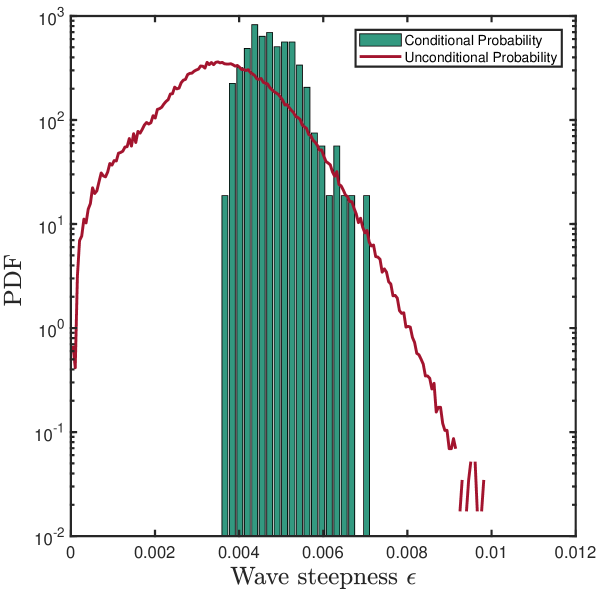
Rogue waves in ocean are sometime described as walls of water. This suggests that rogue waves steepness is large. We probe the correlation between extreme events amplitudes and the wave steepness of the bending waves. The steepness is the ratio of the wave amplitude over half the wavelength, . In terms of the local wave period and height, it can be recast as: , where is the height corresponding to the local period as defined previously. Here, we used the dispersion relation of the bending waves; which remains valid in the nonlinear regime of WT [18]. Figure 9 shows the PDF of the steepness when rare events occurs and compare it to the unconditional steepness PDF. Here again the fluctuations of the rare events steepness are shrunk (about a factor 2) but their average is higher about 30 %. The fact that the steepness of rare events remains of the same order as that of other waves is inconsistent with the ”wall of water” image often derived from sailors’ testimonies, which implies extreme steepness for rogue waves. However, it is important to note that this intuitive picture is not always accurate. Steepness alone may not reliably indicate rogue events, as demonstrated by studies of field measurements from real sea states, which show that normal conditions can also exhibit high wave steepness. [19].
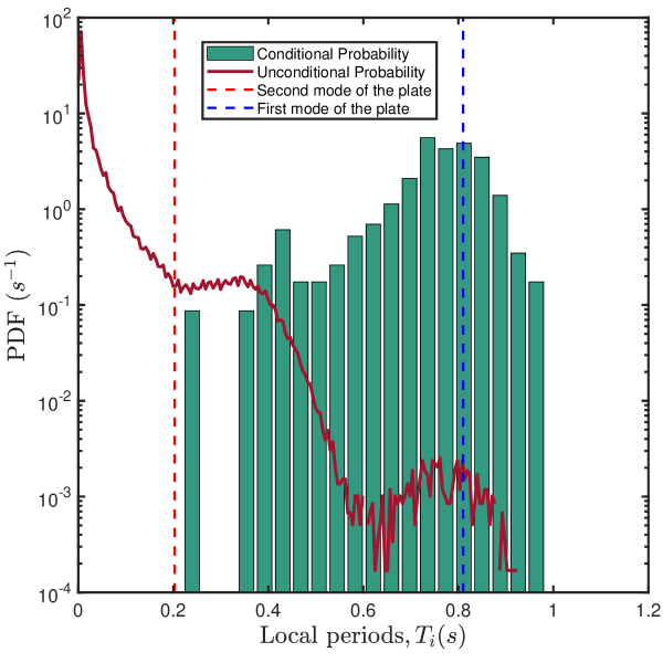
Finally we compare in figure 10 the statistics of the local period of rare events to the unconditional local period statistics. Here the local periods of extreme events are clearly concentrated around the highest periods that coincide with a bump in the unconditional PDF of the local period. These local periods around 0.8 s correspond to nearly 2 m wavelength. It is one wavelength along the length and half a wavelength along the width of the plate. Actually this fundamental mode is clearly visible in the spectra figure 4. All these observations made in the case with and Hz in figures 8 – 10, remains true for all forcing, at 150 and 250 Hz, as long as we are in the nonlinear regime. At 30 Hz where the equipartition stage is reduced, the steepness of rare events is slightly higher. We report in the table in appendix A: the ratio of the unconditioned statistics over the conditioned one for the kinetic energy per unit mass during a period, for the steepness and for the local period for the average and the variance of all our experimental run.
With these elements, we can elaborate the following scenario for the generation of rare events in a set of bending waves. Although there is no inverse cascade expected in the bending wave turbulence, there is at least an equipartiton of the energy per mode at wavelength larger than the forcing in the stationary state. This is enough to bring energy to the fundamental modes of the plate. This large wavelength will not require a high steepness to reach a very large height. The steepness must be slightly higher when the equipatition range is reduced. The extreme events develop over the fundamental modes of the plate. Since these rare events occur over the longest wavelength, their kinetic energy per unit mass during these modes reaches its time average value.
One can conclude that the mechanisms generating extreme events in sea surface and in a set of bending wave are different. We had to use another statistical criterion to recover a fraction of rare events similar to the observation of rogue waves. For the bending waves, the fundamental modes of the elastic plate play a major role, and the rare events correspond to the longest wavelength with our statistical definition of the extreme events. This correlation has not been reported for surface waves. In contrast, the rogue waves occur near the Tayfun period , where the Tayfun frequency is . Here, the mean frequency is , the dimensionless spectral bandwidth is , and the spectral moments are for [20, 1, 5]. Our study raises several issues. For instance, can we use only statistical criteria to characterize completely rogue waves without any consideration about the spectrum of the waves? In other world, can we just assimilate rogue waves to extreme events without consideration of the steepness or the energy? Another issue concern the role of the inverse cascade in the rogue wave’s formation. Indeed, although there is no inverse cascade in the bending waves, the equiparition is enough to fill up the fundamental modes of the plate. The inverse cascade of the wave action must enhance this process for surface gravity waves. However, this phenomenon is not reported in wave tanks where the inverse cascade, if existing, is quite limited [21]. Moreover, the phenomenological JONSWAP spectrum used to describe the sea state is relatively narrow [22]. What is the mechanism limiting the transfer to large wavelength in wave tanks? What implies this cutoff in the extreme events generation?
This study leverages the advantages of bending elastic waves, where we observe extreme states similar to those in surface gravity waves but driven by different mechanisms. By using forcing frequencies nearly 100 times higher than those in surface gravity wave experiments, we can collect much more statistical data in a shorter time. These features provide new insights into the mechanisms behind bending elastic waves, offering a different perspective. Finally, we acknowledge that our current definition of local wave period may not fully capture true rogue waves in a set of bending waves, a point to be addressed once the definition is clarified.
Acknowledgements.
We wish to acknowledge the ANR for financial support and B. Gallet, C. Touzé, S. Varghese for fruitful discussions.Appendixes
Appendix A Tables
| 0.5Vpp | 0.5Vpp(LONG)111Long measurement of 62 hours to check convergence | 1.0Vpp | 1.5Vpp | |
|---|---|---|---|---|
| 00footnotetext: is the r.m.s transversal displacement; | ||||
| 00footnotetext: is the r.m.s injected velocity; | ||||
| K00footnotetext: K is the kurtosis; S is the skewness; | ||||
| S | ||||
| 00footnotetext: is the total number of all recorded events; | ||||
| 00footnotetext: is the number of detected rare events; | ||||
| frac 00footnotetext: frac is the ratio of ; | ||||
| 00footnotetext: and | ||||
| 0.5Vpp | 1.0Vpp | 2.0Vpp | 3.0Vpp | 4.0Vpp | 5.0Vpp | |
|---|---|---|---|---|---|---|
| K | ||||||
| S | ||||||
| frac | ||||||
| 2.0Vpp1115-hour measurement | 3.0Vpp1115-hour measurement | 3.2Vpp1115-hour measurement | 3.4Vpp1115-hour measurement | 3.6Vpp | 3.8Vpp | 4.0Vpp2226-hour measurement | 4.5Vpp | 7.0Vpp | |
|---|---|---|---|---|---|---|---|---|---|
| K | |||||||||
| S | |||||||||
| frac | |||||||||
References
- [1] Nobuhito Mori, Takuji Waseda and Amin Chabchou, ed. Science and Engineering of Freak Waves (Elsevier Inc, 2003) https://doi.org/10.1016/C2021-0-01205-0
- [2] Kristian Dysthe, Harald E. Krogstad and Peter Muller, Oceanic Rogue Waves Annu. Rev. Fluid Mech. 2008.40:287-310
- [3] A. Chabchoub, N. P. Hoffmann, and N. Akhmediev, Rogue Wave Observation in a Water Wave Tank, Phys. Rev. Lett. 106, 204502 (2011), DOI: 10.1103/PhysRevLett.106.204502
- [4] A. Toffoli, D. Proment, H. Salman, J. Monbaliu, F. Frascoli, M. Dafilis, E. Stramignoni, R. Forza, M. Manfrin, and M. Onorato, Wind Generated Rogue Waves in an Annular Wave Flume, Phys. Rev. Lett. 118, 144503 (2017), DOI: 10.1103/PhysRevLett.118.144503
- [5] Guillaume Michel, Félicien Bonnefoy, Guillaume Ducrozet and Eric Falcon, Statistics of rogue waves in isotropic wave fields Journal of Fluid Mechanics , Volume 943 , 25 July 2022 , A26 DOI: https://doi.org/10.1017/jfm.2022.436
- [6] D. H. Peregrine, Water Waves , nonlinear Schrödinger equations and their solutions, Austral. Math. Soc. Ser. B 25 (1983), 16-43 DOI: https://doi.org/10.1017/S0334270000003891
- [7] John M. Dudley, Frédéric Dias, Miro Erkintalo and Goëry Genty Instabilities, breathers and rogue waves in optics, NATURE PHOTONICS 8 (2014), DOI: 10.1038/NPHOTON.2014.220
- [8] M. Onoratoa, S. Residori, U. Bortolozzo, A. Montina , F.T. Arecchi, Rogue waves and their generating mechanisms in different physical contexts, Physics Report 528–2 ‘2013), 47-89
- [9] H. Bailung, S. K. Sharma, and Y. Nakamura, Observation of Peregrine Solitons in a Multicomponent Plasma with Negative Ions, PRL 107, 255005 (2011), DOI: 10.1103/PhysRevLett.107.255005
- [10] S. Nazarenko, Waves Turbuence Lecture Notes in Physics 825, (Springer-Verlag, Berlin 2011)
- [11] L. D. Landau and E. M. Lifshitz, Theory of Elasticity (Pergamon, New York, 1959).
- [12] G. Du’́ring, Ch. Josserand and S. Rica, PRL 97, 025503 (2006)
- [13] N. Mordant, Are There Waves in Elastic Wave Turbulence?, PRL 100, 234505 (2008)
- [14] Arezky Boudaoud, Olivier Cadot, Benoî t Odille, and Cyril Touzé Observation of Wave Turbulence in Vibrating Plates, PRL 100, 234504 (2008)
- [15] T. Humbert, O. Cadot, G. D’́uring, C. Josserand, S. Rica and C. Touzé, Wave turbulence in vibrating plates: The effect of damping, EPL, 102 (2013) ,doi: 10.1209/0295-5075/102/30002
- [16] B Miquel, A Naert, S Aumaître, Low-frequency spectra of bending wave turbulence PHYSICAL REVIEW E 103, L061001 (2021), DOI: 10.1103/PhysRevE.103.L061001
- [17] M. A. Tayfun, Narrow-Band Nonlinear Sea Waves, JOURNAL OF GEOPHYSICAL RESEARCH, 85–C3, pp 1548-1552, (1980)
- [18] P. Cobelli, P. Petitjeans, A. Maurel, V. Pagneux and N. Mordant Space-Time Resolved Wave Turbulence in a Vibrating Plate, Phys. Rev. Lett. 103, 204301 (2009), DOI: 10.1103/PhysRevLett.103.204301
- [19] Christou, M. & Ewans, K. Field Measurements of Rogue Water Waves. Journal Of Physical Oceanography. 44, 2317 - 2335 (2014), https://journals.ametsoc.org/view/journals/phoc/44/9/jpo-d-13-0199.1.xml
- [20] M. A. Tayfun, Joint distribution of large wave heights and associated periods ,Journal of Waterway, Port, Coastal and Ocean Engineering ·(1993) DOI: 10.1061/(ASCE)0733-950X(1993)119:3(261)
- [21] E. Falcon, G. Michel, G. Prabhudesai, A. Cazaubiel, M. Berhanu, N. Mordant, S. Aumaître, and F. Bonnefoy, , Phys. Rev. Lett. 125, 134501, DOI:https://doi.org/10.1103/PhysRevLett.125.134501
- [22] Hasselmann K., T.P. Barnett, E. Bouws, H. Carlson, D.E. Cartwright, K. Enke, J.A. Ewing, H. Gienapp, D.E. Hasselmann, P. Kruseman, A. Meerburg, P. Mller, D.J. Olbers, K. Richter, W. Sell, and H. Walden. Measurements of wind-wave growth and swell decay during the Joint North Sea Wave Project (JONSWAP)’ Ergnzungsheft zur Deutschen Hydrographischen Zeitschrift Reihe, A(8) (Nr. 12), p.95, 1973.