Chemical potential of the warm dense electron gas from ab initio
path integral Monte Carlo simulations
Abstract
We present extensive new ab initio path integral Monte Carlo (PIMC) simulation results for the chemical potential of the warm dense uniform electron gas (UEG), spanning a broad range of densities and temperatures. This is achieved by following two independent routes, i) based on the direct estimation of the free energy [Dornheim et al., arXiv:2407.01044] and ii) using a histogram estimator in PIMC simulations with a varying number of particles. We empirically confirm the expected inverse linear dependence of the exchange–correlation (XC) part of the chemical potential on the simulated number of electrons, which allows for a reliable extrapolation to the thermodynamic limit without the necessity for an additional finite-size correction. We find very good agreement (within ) with the previous parametrization of the XC-free energy by Groth et al. [Phys. Rev. Lett. 119, 135001 (2017)], which constitutes an important cross validation of current state-of-the-art UEG equations of state. In addition to being interesting in its own right, our study constitutes the basis for the future PIMC based investigation of the chemical potential of real warm dense matter systems starting with hydrogen.
I Introduction
Understanding warm dense matter (WDM) – an extreme state characterized by high densities, temperatures, and pressures Graziani et al. (2014); Bonitz et al. (2020); Drake (2018) – constitutes a formidable challenge for theory and experiment alike Bonitz et al. (2024). In nature, such conditions abound in a great variety of astrophysical objects such as giant planet interiors Benuzzi-Mounaix et al. (2014); Vorberger et al. (2007), brown dwarfs Becker et al. (2014), and white dwarf atmospheres Saumon et al. (2022). In addition, WDM plays an important role in several technological applications Kraus et al. (2016); Brongersma et al. (2015). A prime example is inertial confinement fusion (ICF) Hurricane et al. (2023); Betti and Hurricane (2016), where both the fusion fuel and its surrounding ablator material have to traverse the WDM regime in a controlled way Hu et al. (2011), while avoiding incipient inhomogeneities and instabilities. Consequently, a rigorous theoretical understanding of WDM is indispensable for the integrated multi-scale modelling of ICF applications which, in turn, is needed for the development of improved designs with an increased fusion yield to make ICF an economically viable future source of clean and abundant energy Batani et al. (2023).
In the laboratory, WDM is created using a plethora of different techniques Falk (2018) at large research facilities such as the National Ignition Facility (NIF) Moses et al. (2009); Döppner et al. (2023); MacDonald et al. (2023), the Linac Coherent Light Source (LCLS) Bostedt et al. (2016); Glenzer et al. (2016), and the OMEGA laser facility Soures et al. (1996); Glenzer et al. (2007) in the USA, the Laser Megajoule Miquel et al. (2016) in France, and the European XFEL Tschentscher et al. (2017) in Germany. Here, a major challenge is given by the rigorous diagnostics of the extreme states of matter generated, which is further exacerbated by the ultrafast time scales (typically s). In practice, even the most advanced inelastic x-ray scattering methods Glenzer and Redmer (2009); Sheffield et al. (2010); Fletcher et al. (2015) typically depend on approximate theoretical models for their interpretation Gregori et al. (2003); Döppner et al. (2023); Böhme et al. (2023); Fletcher et al. (2022); Sperling et al. (2015). Although there has been noteable recent progress both in the model-free interpretation of x-ray Thomson scattering (XRTS) measurements Dornheim et al. (2022a, 2023a, 2024a, 2024b); Vorberger et al. (2024) and in the more rigorous modelling based on ab initio simulations Schörner et al. (2023); Dornheim et al. (2024c); Gawne et al. (2024); Kononov et al. (2022), the value of these experiments for the determination of key properties such as the equation-of-state (EOS) of a given material Falk et al. (2014, 2012) has remained limited; an improved theoretical description is therefore strongly needed.
From a theoretical perspective, WDM is more conveniently defined by two dimensionless parameters that are both of the order of unity Ott et al. (2018); Dornheim et al. (2023b): the density parameter with the number density, and the degeneracy temperature with the usual electronic Fermi energy Giuliani and Vignale (2008); a third parameter is given by the classical coupling parameter of the ions that indicates the ratio of Coulomb interaction to ionic kinetic energy, and is also of the order of or even larger than one. This implies the nontrivial interplay of effects such as Coulomb coupling, strong thermal excitations, quantum degeneracy and diffraction, and, in general, also partial ionization that have to be taken into account holistically. In thermal equilibrium, the gold standard for the modelling of quantum many-body systems such as WDM is given by quantum Monte Carlo (QMC) methods Anderson (2007), with the ab initio path integral Monte Carlo (PIMC) approach Herman et al. (1982); Pollock and Ceperley (1984); Takahashi and Imada (1984) often being the method of choice at finite temperatures.
In this context, a key system is given by the uniform electron gas (UEG) Giuliani and Vignale (2008); Dornheim et al. (2018a); Loos and Gill (2016), which is the archetypal system of interacting electrons and constitutes the quantum mechanical generalization of the classical one-component plasma. In the ground state, QMC results for the UEG Ceperley and Alder (1980); Ortiz and Ballone (1994); Ortiz et al. (1999); Moroni et al. (1992, 1995); Spink et al. (2013) have been pivotal for the arguably unrivaled success of density functional theory (DFT) in statistical physics, quantum chemistry, material science, and related disciplines Jones (2015). Over the last decade, these efforts have been extended to WDM conditions Brown et al. (2013); Schoof et al. (2015); Filinov et al. (2015); Dornheim et al. (2016); Groth et al. (2017a); Malone et al. (2015, 2016); Yilmaz et al. (2020); Hou et al. (2022); Lee et al. (2021), resulting in extensive results for a wealth of UEG properties such as its linear Dornheim et al. (2019a); Hou et al. (2022); Groth et al. (2017b); Dornheim et al. (2020a, b, 2021a, 2022b) and non-linear Dornheim et al. (2020c, 2021b, 2021c, 2021d) density response, its structural properties Dornheim et al. (2017, 2016); Brown et al. (2013), its momentum distribution function Hunger et al. (2021); Dornheim et al. (2021e, f); Militzer and Pollock (2002); Militzer et al. (2019), its virial coefficients Dornheim et al. (2022c); Röpke et al. (2024), its imaginary-time structure Dornheim et al. (2023c, d, e), and even its dynamic structure factor Dornheim et al. (2018b); Groth et al. (2019); Dornheim et al. (2022d); Filinov et al. (2023) and dynamic Matsubara density response Tolias et al. (2024a); Dornheim et al. (2024d, e, f). Of particular value are the accurate parametrizations of its exchange–correlation (XC) free energy Groth et al. (2017a); Dornheim et al. (2018a); Karasiev et al. (2014, 2019) that continuously cover the entire relevant WDM phase diagram region. These XC-functionals can be used directly as input for thermal DFT simulations Mermin (1965) of real WDM applications on the level of the local density approximation Karasiev et al. (2016); Sjostrom and Daligault (2014); Ramakrishna et al. (2020), and as the basis for the construction of more advanced functionals Sjostrom and Daligault (2014); Karasiev et al. (2018, 2022); Kozlowski et al. (2023).
In practice, the construction of the two most important parametrizations – the functional by Groth et al. Groth et al. (2017a) (GDSMFB) and the corrected functional by Karasiev et al. Karasiev et al. (2018, 2014) (corrKSDT) – is based on PIMC results for the interaction energy , kinetic energy , or internal energy (or a combination of these three) as well as on thermodynamic relations such as the well-known adiabatic connection formula Ichimaru et al. (1987). This was necessary as PIMC by itself does not give one direct access to the partition function , with the total particle number, the volume of the cubic simulation cell, and the inverse temperature in energy units, thus precluding direct access to the free energy
| (1) |
Very recently, four of us have changed this rather unfortunate situation by introducing simulations in the extended -ensemble Dornheim et al. (2024g). This new scheme connects a non-interacting and uniform Bose reference system, for which the canonical partition function and free energy can be readily estimated from a well-known recursion relation Krauth (2006); Barghathi et al. (2020); Zhou and Dai (2018), with the interacting (and, in general, potentially non-uniform) system of interest and, in this way, allows for the direct estimation of the free energy from PIMC simulations for a single density–temperature combination, i.e., without thermodynamic integration. The subsequent extensive application of this idea to the warm dense UEG Dornheim et al. (2024h) has fully substantiated the high quality of the GDSMFB parametrization, which constitutes a valuable independent cross-check of this key property.
In the present work, we consider another important thermodynamic property: the chemical potential that describes the change in the free energy upon adding an additional particle to the system. In general, the accurate knowledge of is crucial for understanding the stability conditions of complex systems. Indeed, the chemical potential governs the stability of multiphase systems (it yields the phase coexistence line), the chemical stability (equilibrium between reaction products, mass action law) and the stable density profile in an external field. Moreover, the chemical potential provides some insight into the electronic properties. Since it is related to the energy needed to add particles to the system, , it contains information about the binding energy and the energy of the highest occupied orbital (HOMO) in a quantum system either in the ground state or in the presence of a band gap that is larger than the thermal energy. In finite systems, such as nuclei, Coulomb clusters Tsuruta and Ichimaru (1993); Ludwig et al. (2005); Bonitz et al. (2010), ions in traps Dubin and O’Neil (1999) or artificial atoms Ashoori (1996); Bedanov and Peeters (1994), is directly related to the addition energy and to the electronic structure (shell configuration, magic clusters etc.). In a macroscopic Fermi system in the ground state, it coincides with the Fermi energy. We underline that this applies not only to ideal models, but also to interacting systems, where the Fermi energy is generally not known. Therefore, a first-principles approach to the chemical potential will be extremely valuable, in particular for warm dense matter.
In classical systems, the chemical potential has been computed from numerical simulations using free energy perturbation methods Bennet (1976), Widom insertion methods Kofke and T. (1997), expanded ensemble methods Attard (1993), histogram-reweighting methods S. and E. (1982) or spatially resolved thermodynamic integration methods Heidari et al. (2018). Most widespread are the free energy perturbation methods that are based on the Zwanzig identity Zwanzig (1954) and the closely related Widom insertion methods that are based on the potential distribution theorem Widom (1982); Bakhshandeh and Levin (2022). Dedicated umbrella sampling techniques and multistage variants of these methods have been developed with the objective of increasing the sampling efficiency for dense liquids Kofke and T. (1997); Heidari et al. (2018). However, the theoretical backbone of most of these methods (the Zwanzig identity or the potential distribution theorem) cannot be straightforwardly extended to quantum systems, (i) being based on the classical factorization which does not generally hold, since the kinetic and potential energy operators do not commute, and (ii) not considering the proper Fermi-Dirac (or Bose-Einstein) statistics Herdman et al. (2014). Here, we use exact PIMC simulations to compute in two independent ways, namely by computing the difference in the free energy [Eq. (2)] using our recent -ensemble approach and also by estimating the corresponding ratio of - and particle partition functions from a single simulation in which the number of particles is allowed to vary. We find perfect agreement between these routes, as it is expected.
A great practical advantage of the chemical potential concerns its known scaling with respect to the number of electrons Herdman et al. (2014); Siepmann et al. (1992) towards the thermodynamic limit (TDL), i.e., the limit of where is being kept constant. This allows us to reliably extrapolate our PIMC results to the TDL without the need for the usual semi-analytical finite-size corrections Chiesa et al. (2006); Drummond et al. (2008); Brown et al. (2013); Dornheim et al. (2016); Dornheim and Vorberger (2021); ueg ; Holzmann et al. (2016) that have been used for the construction of the GDSMFB and corrKSDT parametrizations, but also for the finite-size correction of the new free energy results in Refs. Dornheim et al. (2024g, h). The present estimation of [and its XC-contribution thus constitutes a completely independent route towards the EOS of a given system, and thus allows us to further test previous results over a broad range of densities and temperatures. In addition to its considerable value for the further understanding of the archetypal UEG, the present study will serve as a template for the future PIMC based investigation of the chemical potential of real WDM systems such as hydrogen Filinov and Bonitz (2023); Bonitz et al. (2024); Dornheim et al. (2024i); Böhme et al. (2022); Militzer and Ceperley (2001); Militzer et al. (2021) and beryllium Dornheim et al. (2024c).
The paper is organized as follows: In Sec. II, we give a concise overview of the required theoretical background, including an introduction to the chemical potential (Sec. II.1), to the direct PIMC estimation of the free energy via the extended -ensemble (Sec. II.2), to the estimation of the canonical properties of the ideal Bose gas and ideal Fermi gas (Sec. II.3), to the decomposition of the total chemical potential into an ideal, a bosonic interaction, and a quantum statistical contribution (Sec. II.4), to the alternative histogram estimator route (Sec. II.5), and to the estimation of based on parametrizations of (II.6). All simulation results are presented in Sec. III, starting with the verification and comparison of the independent PIMC estimators (III.1) and an exploration of the required extrapolation to the thermodynamic limit (Sec. III.2); the bulk of our results is presented in Sec. III.3, where we compare the present data to the previous parametrization by Groth et al. Groth et al. (2017a). The paper is concluded by a summary and outlook in Sec. IV.
II Theory
We assume Hartree atomic units throughout this work unless indicated otherwise. Detailed introductions to the PIMC method Ceperley (1995); Boninsegni et al. (2006a), its application to the UEG Dornheim et al. (2018a, 2019b), and the associated fermion sign problem Dornheim (2019) have been presented in the literature.
II.1 Chemical potential
In the canonical ensemble, which is defined by a constant number of particles , volume and inverse temperature , the chemical potential is given by the change in the free energy associated with the addition of a particle, ,
| (2) |
with the free energy related to the canonical partition function by the usual relation, Eq. (1). While both and cannot be directly estimated within a traditional PIMC simulation, one can obtain both by connecting the interacting (and, in general, also inhomogeneous) system of interest with a non-interacting reference system for which both and are known Dornheim et al. (2024g, h), see Sec. II.2 below.
For simulations with periodic boundary conditions, it has become a standard practice to use the Ewald pair interaction potential, which constitutes the corresponding solution of Poisson’s equation Fraser et al. (1996). In this situation, the definition of Eq. (2) is somewhat ambiguous. Specifically, one might either add a Coulomb interacting electron (i.e., without the infinite periodic array of images), or an additional Ewald interacting electron with its own neutralizing background. Bakhshandeh and Levin Bakhshandeh and Levin (2022) have shown that, for classical systems, while both approaches converge to the same TDL, the latter exhibits a more favorable converge behavior. In the present quantum case, it is important that the added electron is indistinguishable from the other electrons (of the same spin orientation), which makes the neutralized Ewald potential the appropriate choice.
II.2 Free energy and the -ensemble
To compute the free energy from PIMC simulations, we follow the approach introduced in Refs. Dornheim et al. (2024g, h) and consider the modified Hamiltonian
| (3) |
where and denote the operators of kinetic and potential energy, respectively. Here denotes a free parameter, with describing a non-interacting reference system and corresponding to the non-ideal system of interest. By connecting these two limits (with intermediate steps), one can access the free energy of the interacting Fermi system via Dornheim et al. (2024g)
with the free energy of an ideal Bose gas that can be computed from a recursion relation for the corresponding canonical partition function, cf. Eq. (6) below. The second term on the RHS of Eq. (II.2) connects the ideal and non-ideal Bose systems, with being the ratio of configurations with two different -values, and with being a free algorithmic parameter; see Ref. Dornheim et al. (2024h) for an extensive discussion. The final term is given by the average sign
| (5) |
which constitutes an important measure for the degree of cancellation between positive and negative contributions in a PIMC simulation with a sign problem Dornheim (2019), and which, in the context of the present work, constitutes a quantum statistics correction connecting the interacting Bose and Fermi systems.
II.3 Ideal Fermi and Bose gas
The final missing ingredient is given by . For this purpose, we use the well-known recursion relation of the canonical partition function of ideal quantum many-body systems Barghathi et al. (2020); Krauth (2006); a convenient compact form for spin-polarized bosons or fermions is given by Zhou and Dai (2018)
| (6) |
with the matrix being defined as
| (7) |
with ; note that and in the first line of Eq. (7) correspond to Fermi-Dirac and Bose-Einstein statistics, respectively. In the noninteracting case, the partition functions of the individual spin-components factorize (this holds even in the spin-polarized case with and , as it is ), and the full partition function is given by
| (8) |
It is easy to see that the chemical potential can be expressed as the ratio of partition functions Herdman et al. (2014); Hansen and McDonald (2013)
| (9) |
the ideal chemical potential that corresponds to the addition of a spin-up particle is thus given by
| (10) |
as all spin-down contributions trivially cancel. Naturally, Eq. (10) does not generalize to interacting systems.
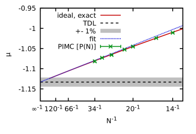
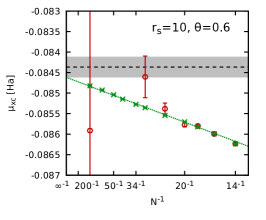
In the top panel of Fig. 1, we show the canonical chemical potential of the unpolarized ideal Fermi gas at and as a function of the total number of particles. Specifically, the solid red line corresponds to Eq. (10) and the dashed black line depicts the thermodynamic limit, i.e., the limit of as the density is being kept constant. We note that the evaluation of the determinant in Eq. (6) becomes unstable for at these conditions. The dotted blue line shows an empirical linear fit to the canonical results for and leads to good agreement with the correct thermodynamic limit. The PIMC results for that are also shown in Fig. 1 are discussed in Sec. II.5 below.
II.4 Decomposition of the chemical potential
Taken together, we can express the chemical potential of the non-ideal Fermi system of interest as
| (11) |
which consists of three individual contributions that are defined in analogy to the decomposition of the total free energy introduced in Ref. Dornheim et al. (2024h):
| (12) | |||||
In a nutshell, the full chemical potential is given by the sum of the chemical potential of the ideal Bose system , the bosonic interaction contribution , and the quantum statistical contribution .
II.5 Chemical potential from particle number histograms
As an alternative route towards the chemical potential of interacting quantum many-body systems, we can estimate the corresponding ratio of canonical partition functions [Eq. (9)] from PIMC simulations where the particle number is allowed to vary. For example, one might consider the grand-canonical partition function
| (13) |
where the grand-canonical chemical potential is a free input parameter. The canonical expectation value of then immediately follows as Herdman et al. (2014)
| (14) |
with being the histogram of particle numbers, i.e., the expectation value of the operator
| (15) |
in the grand-canonical simulation, with being the particle number of the PIMC configuration ; hence,
| (16) |
We note that, for a fermionic PIMC simulation that is subject to the fermion sign problem Dornheim (2021), the grand-canonical expectation value in Eq. (16) is given by
| (17) |
with the grand-canonical average sign Dornheim (2021), and where the notation implies the usual expectation value with respect to the bosonic absolute weights Dornheim (2019, 2021).
On one hand, the histogram approach given in Eq. (14) has the advantage that one can get from a single PIMC simulation, and without the need for any external input for the noninteracting Bose- or Fermi-system. On the other hand, a substantial amount of simulation time might be wasted for particle numbers or that are not relevant for the evaluation of Eq. (14). To remedy this issue, we generalize Eq. (13) as
| (18) |
leading to
| (19) |
A convenient empirical choice for the generalized weight function is given by
| (20) |
with being the target number of particles; the variance controls the amount of irrelevant particle numbers in the PIMC simulation, with being a good choice. This leads to our final result for the canonical chemical potential,
| (21) |
Without loss of generality, we employ the full grand-canonical worm algorithm Boninsegni et al. (2006b, a) to update the spin-up electrons, which are allowed to vary with respect to the number of particles. In contrast, we use a canonical adaption of the worm algorithm Dornheim et al. (2021e) to update the spin-down electrons, for which the number of particles is being kept fixed.
In practice, we find that the histogram approach constitutes a more convenient and efficient route towards and we use it for the bulk of the warm dense UEG results that are presented below. The direct free energy approach is less efficient, but it constitutes a valuable and independent cross check of our implementation.
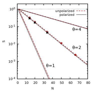
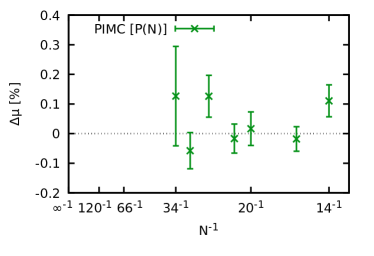
The green crosses in the top panel of Fig. 1 show PIMC results that have been computed via Eq. (21) for . They are in excellent agreement with the exact reference curve within the given statistical confidence interval; this can be seen particularly well in the bottom panel of Fig. 1, where we show the relative deviation of the PIMC data from the exact result. We find increasing error bars upon increasing the system size, which is a direct consequence of the inherent cancellation of positive and negative terms due to the fermion sign problem Dornheim (2019, 2021). In Fig. 2, we show the average sign [Eq. (5)] of the ideal Fermi gas as a function of the system size both for the unpolarized (dashed red) and spin-polarized (dotted black) cases for , , . In all three cases, we find the expected exponential decrease with Troyer and Wiese (2005); Dornheim (2019), which illustrates the challenges associated with the PIMC simulation of quantum degenerate Fermi systems. Fortunately, the sign problem is considerably less severe for interacting systems, since Coulomb repulsion effectively suppresses the formation of permutation cycles Dornheim et al. (2019b); this holds both for the extended -ensemble and the histogram estimator. The red circles and black stars in Fig. 2 show PIMC results for both spin polarizations for and are in perfect agreement with the exact, semi-analytical result, as expected.
II.6 Chemical potential from the UEG equation-of-state
To utilize available parametrizations of the free energy in terms of and , we need to perform a derivative of the free energy with respect to the density under constant temperature and volume. We define the free energy per particle , leading to
| (22) |
The derivative of the free energy with respect to the density at constant temperature can be obtained from a parametrization in and by considering the derivative of a function f(x) in the direction given by vector . Using the connection between and for constant temperature , it follows
| (23) |
The chemical potential is then
| (24) |
Naturally, the same relation holds between the respective XC-contributions and .
III Results
All PIMC results that are presented in this work have been computed using the open-source ISHTAR code Dornheim et al. (2024j), and were obtained for a fully unpolarized system. We use imaginary-time propagators within the primitive factorization , and the convergence with the number of time slices has been carefully checked. More sophisticated factorization schemes Sakkos et al. (2009) and their application to Fermi systems Chin (2015); Dornheim et al. (2015) have been presented in the literature, but they are not required here. Note that we do not impose any nodal restrictions Ceperley (1991), which makes our simulations very costly due to the fermion sign problem Dornheim (2019), but exact within the given Monte Carlo error bars.
III.1 Verification and comparison of estimators
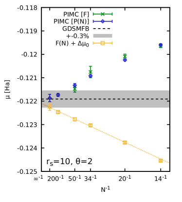
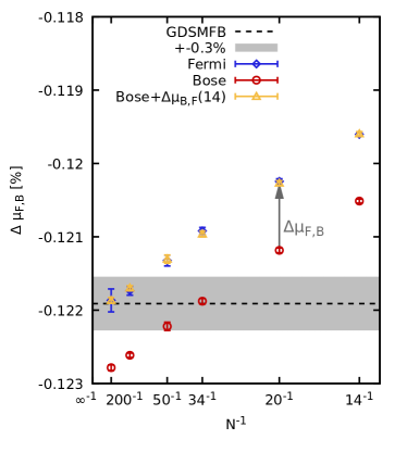
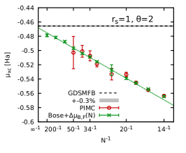
In the left panel of Fig. 3, we show PIMC simulation results for the total canonical chemical potential as a function of the total number of electrons for the unpolarized UEG at and . The dashed black line has been obtained from the parametrization of by Groth et al. Groth et al. (2017a) (GDSMFB), and has been included as a reference; the shaded grey area shows an interval of around this result and serves as a guide to the eye. The green crosses have been obtained by directly evaluating the differences in the free energy [Eqs. (2) and (11)] and appear to converge towards the GDSMFB reference result. The blue diamonds show independent PIMC results from the histogram estimator [Eq. (21), with ] and are in excellent agreement with the independent -ensemble results for all within the given Monte Carlo error bars. Importantly, the latter are considerably smaller for the histogram estimator, making it the method of choice throughout the remainder of this paper.
The yellow squares have been computed from the blue diamonds by finite-size correcting the non-interacting part, i.e., by adding the corresponding finite-size correction
| (25) |
Interestingly, adding the correction Eq. (25) to the raw PIMC results does not diminish the magnitude of the dependence on the system size, but changes its sign. Nevertheless, adding is very advantageous in practice as the asymptotic dependence of the XC-contribution to on the number of electrons has been presented in the literature Siepmann et al. (1992); Herdman et al. (2014),
with being the total pressure. The dotted yellow line shows a corresponding linear fit for , which nicely captures the functional dependence of the PIMC results. Eq. (III.1) thus constitutes a reliable route to extrapolate our PIMC results for to the appropriate thermodynamic limit without the need for any external finite-size correction.
The right panel of Fig. 3 is devoted to the analysis of quantum statistics effects. Specifically, the blue diamonds and red circles show our raw PIMC results for Fermi-Dirac and Bose-Einstein statistics, respectively. In addition, the yellow triangles have been obtained by adding to the red circles a constant quantum statistics correction that has been computed for electrons. Evidently, the thus obtained data points are in perfect agreement with the full fermionic PIMC results, but with a substantially reduced statistical error bar. Naturally, the impact of quantum statistics becomes more pronounced for higher density and lower temperatures, and the utility of a corresponding decomposition [cf. Eq. (11)] is investigated in the following.
III.2 Decomposition and extrapolation to the thermodynamic limit
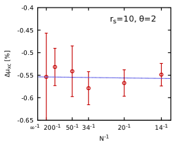
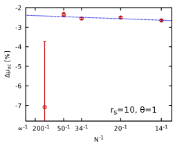
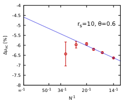
In Fig. 4, we show the quantum statistical contribution , i.e., the difference between the chemical potential obtained for Fermi-Dirac and Bose-Einstein statistics, as a function of system size for various combinations of the density and temperature. Note that we normalize these differences by the computed from the GDSMFB parametrization Groth et al. (2017a) for convenience. The top row has been obtained for and (left), (center), and (right), i.e., for typical WDM parameters. Remarkably, we find differences exceeding in between fermions and bosons for , which clearly emphasizes the importance of quantum degeneracy effects for the description of WDM. At the same time, the dependence of on is relatively weak for all depicted cases. This also holds for the bottom row, where we show results for , which corresponds to the boundary of the strongly coupled electron liquid regime Dornheim et al. (2020a, 2018b), for (left), (center) and (right).
This observation is of great practical value, since PIMC simulations of large bosonic systems are comparatively unproblematic, as they are not subject to the exponential increase in compute time due to the fermion sign problem. We thus propose to use bosonic PIMC results for as a basis, and to correct them with PIMC results for that can be estimated reliably for a significantly smaller number of particles. In practice, we use an empirical linear model for , which is included as the dotted blue lines in Fig. 4; we find excellent agreement between the PIMC results and these fits for all investigated cases, and over the entire investigated range of system sizes .
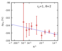
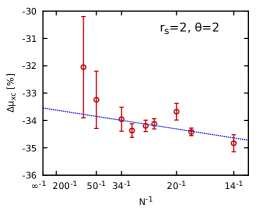
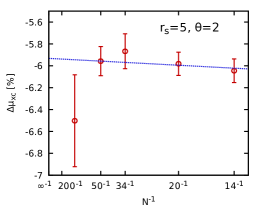
Let us next consider Fig. 5, where we investigate the extrapolation of to the TDL for the same parameters as in Fig. 4. Overall, we find the most pronounced dependence on the system size for the highest density ( and ), where the finite-size effect for attains roughly one half of in the TDL. In contrast, finite-size effects decrease towards lower temperatures and larger , which is consistent with the investigation of the finite-size effects of other observables in the available literature Dornheim et al. (2016, 2018a, 2020d, 2024h). More specifically, the red circles show our raw fermionic PIMC results; these are very accurate for small , but exhibit substantially increasing statistical error bars with increasing due to the fermion sign problem, in particular at high densities and low temperatures. In stark contrast, the green crosses that have been obtained by adding to the bosonic PIMC results the quantum statistical correction as it has been explained in the discussion of Fig. 4 above, are not afflicted by this exponential scaling and remain accurate even for . This allows us to reliably extrapolate to the TDL, see the dotted green curves that correspond to linear fits for motivated by Eq. (III.1). We again stress that this procedure does not involve any of the usual external finite-size correction procedures that have been applied for the construction of both GDSMFB and corrKSDT (as well as to the original KSDT Karasiev et al. (2014), albeit in a truncated first-order form Brown et al. (2013); Dornheim et al. (2016)).
III.3 Comparison to previous parametrization
Let us conclude our investigation by comparing our new extrapolated results for [see also Table 1] to the state-of-the-art parmetrization of by Groth et al. Groth et al. (2017a) (GDSMFB). We note that the corrected KSDT functional (corrKSDT) is largely indistinguishable from GDSMFB Karasiev et al. (2019), so that our conclusions can be expected to hold for both parametrizations.
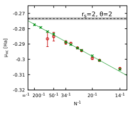
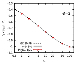
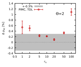
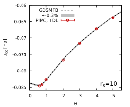
In the top row of Fig. 6, we first investigate the -dependence of for a constant value of the degeneracy temperature of . The top left panel shows the results for itself (multiplied by for convenience), with the dashed black line corresponding to GDSMFB and the red circles to our new results. Clearly, both data sets exhibit the same qualitative behavior over the depicted range of densities. To get a more quantitative comparison, we show the relative deviation in the central panel. The largest deviation between GDSMFB and the present work is given by at . Indeed, GDSMFB has been based on configuration PIMC and permutation blocking PIMC input data for , which makes the good agreement so far out of its range of application all the more impressive. A second trend is given by the systematic sign of the observed deviation, which is always positive; in other words, the new PIMC results are always somewhat smaller than the result computed from GDSMFB at , even though this deviation is small in magnitude. In fact, GDSMFB boasts a relative accuracy of Groth et al. (2017a) (which has inspired the shaded gray area in Fig. 6), but this can be expected to translate into a larger uncertainty for its derivatives. This point has been investigated recently by Karasiev et al. Karasiev et al. (2019), who found unphysical oscillations in the heat capacity computed from either GDSMFB or corrKSDT. On the other hand, this discrepancy might also stem from the present work, possibly from the extrapolation to the thermodynamic limit. Indeed, while the asymptotic -dependence seems to empirically hold for based on our PIMC data, a small residual second-order effect might induce a systematic bias in , which might also explain the observed small deviations. Here, we cannot conclusively resolve this intriguing question at these conditions; the observed agreement on the order of is well within the expected accuracy range for a derivative of GDSMFB and is thus satisfactory. For completeness, we show the relative importance of quantum statistical effects in the right panel. Evidently, it quickly decays with decreasing density where the formation of permutation cycles is suppressed by the increasing degree of Coulomb repulsion, and it becomes negligible in the electron liquid regime.
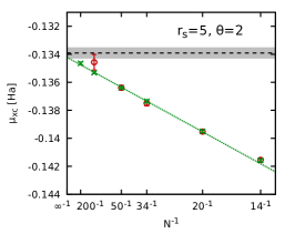
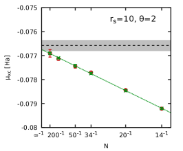
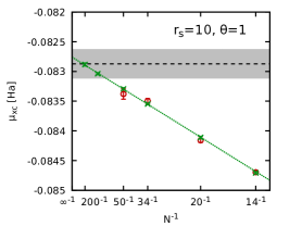
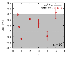
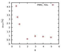
In the bottom row of Fig. 6, we investigate the -dependence of at , for which GDSMFB exhibits a nontrivial minimum around . A similar non-monotonic behavior has been observed by Groth et al. Groth et al. (2016) for the XC-energy , where it has been explained as a competition between quantum delocalization and thermal disorder, which increases towards low and high temperatures, respectively. While our PIMC simulations are limited to , we can clearly resolve a lower value for at compared to the zero-temperature limit. In the center panel of the bottom row, we show again the relative deviation between the present work and GDSMFB. Evidently, all new PIMC data points are in good agreement with the interval around the latter, including the lowest temperature point at . This regime constitutes the most uncertain part of GDSMFB, where its functional dependence has been determined based on temperature-corrected STLS data points Groth et al. (2017a). Finally, the quantum statistical contribution that is depicted in the right panel systematically increases towards low temperatures, and attains at at this relatively low density.
IV Summary and Discussion
In this work, we have presented extensive new ab initio PIMC results for the chemical potential of the warm dense UEG. To this end, we have implemented two independent strategies: i) the direct estimation of as the change in free energy by computing the latter for both and particles using the recent extended -ensemble approach Dornheim et al. (2024g, h) and ii) the estimation of from the ratio of the corresponding partition functions based on PIMC simulations with a varying particle number. In practice, both routes give the same results, with the histogram estimator being the more efficient choice. A great advantage of the chemical potential compared to other thermodynamic observables such as the free energy , internal energy , or kinetic/interaction energy and is its a-priori known asymptotic dependence on the system size Siepmann et al. (1992); Herdman et al. (2014). In combination with the decomposition of into an easy to compute bosonic contribution and an additional quantum statistical correction that can be estimated from relatively small system sizes, this has facilitated the reliable extrapolation to the thermodynamic limit based on PIMC results for up to electrons. This has been achieved without the need for any additional external finite-size corrections, as those employed for the construction of previous PIMC based parametrizations of the UEG EOS.
Overall, we find a very good agreement between the present results and the XC-contribution to computed from the XC-free energy parametrization by Groth et al. Groth et al. (2017a). More specifically, we have found a maximum deviation of at , which, however, is well outside the nominal applicability range of GDSMFB. For , we observe a maximum deviation of at , with a small but systematic trend for all densities at . This could fully be explained by the nominal confidence interval of reported by Groth et al. Groth et al. (2017a), which can easily be exceeded by the evaluation of the derivatives both with respect to and that are required for the estimation of [cf. Eq. (24)]. An alternative potential explanation is given by a small residual term in our extrapolation to the TDL; this, however, cannot conclusively be resolved based on the given data. On the other hand, we find no such systematic trend for the -dependence at . We, thus, conclude that the present study constitutes a valuable independent cross check of current state-of-the art parametrizations of the UEG, which has further substantiated the high quality of the latter.
We are convinced that our work opens up new avenues for a gamut of future investigations. First, we note that the current simulation set-up might be further optimized towards the simulation of larger systems e.g. by utilizing an improved Monte Carlo treatment of the long-range Ewald interaction Müller et al. (2023) or by exploiting path contraction schemes John et al. (2016). Moreover, one might pursue a more efficient estimation of quantum statistics effects by combining the histogram estimator for with the -extrapolation technique Xiong and Xiong (2022); Dornheim et al. (2023f, 2024k), which has been shown to yield highly accurate results for weak to moderate degrees of quantum degeneracy. In addition, we note that constitutes a hitherto unexplored and independent alternative route towards the EOS and can, thus, be used as an additional input for the future construction of improved parametrizations that might yield superior accuracy for the evaluation of derivatives compared to current ones Karasiev et al. (2019). In a similar vein, our set-up can easily be applied to interesting parameter regimes such as the strongly coupled electron liquid regime Dornheim et al. (2020a); Tolias et al. (2021, 2023); Castello et al. (2022), which are outside of the application range of either GDSMFB or corrKSDT. Moreover, we envision the application of our set-up to real WDM systems starting with light elements such as hydrogen. This will facilitate the rigorous assessment of existing EOS tables Militzer et al. (2021) with respect to thermodynamic consistency, and open the way towards the construction of improved parametrizations based on simulation data without the usual approximations e.g. due to a fixed nodal structure (restricted PIMC) or an XC-functional (DFT). Specifically, PIMC reference data for can be utilized to benchmark DFT results for various XC functionals. This will help to avoid problems associated with the dependence of the total free energy on the reference energy of the atoms in DFT, which can vary depending on the type of pseudopotentials used Lejaeghere et al. (2016); Kresse and Hafner (1994); Vanderbilt (1990).
Finally, knowledge of the chemical potential opens up the Gibbs–Duhem route to the isothermal compressibility Attard (2002). To be more specific, an immediate consequence of the Gibbs–Duhem thermodynamic equation reads as Widom (2002); Attard (2002); Lomba and Lee (1996)
| (27) |
Introducing the isothermal coefficient of compressibility , one directly obtains Attard (2002); Lomba and Lee (1996)
| (28) |
Switching from the phase variables to the phase variables, one gets
| (29) |
Within a finite difference approximation of the first order thermodynamic derivatives, the isothermal compressibility can, thus, be evaluated with the histogram approach from four adjacent state point PIMC simulations. The Gibbs–Duhem route is preferable to the free energy route to the isothermal compressibility based on Giuliani and Vignale (2008)
| (30) |
which, thus, also involves all possible second order derivatives with respect to , i.e. Tolias et al. (2024b),
| (31) |
The Gibbs-Duhem route is also preferable to the direct route to the isothermal compressibility through the evaluation of the particle number fluctuations Hansen and McDonald (2013); Balescu (1975)
| (32) |
in grand-canonical ensemble PIMC simulations, since these are generally subject to a severe fermion sign problem in WDM conditions Dornheim (2021). Finally, the Gibbs-Duhem route is also preferable to the sum rule route to the isothermal compressibility, which is based on the exact long-wavelength limit of the static local field correction Giuliani and Vignale (2008)
| (33) |
and involves the exchange-correlation contribution to the isothermal compressibility . The issue here is that the length scales which are relevant to the long wavelength limit are generally inaccessible in PIMC simulations due to the electrons simulated. However, the state-of-affairs is improving with the development of the PIMC extrapolation technique Xiong and Xiong (2022); Dornheim et al. (2023f, 2024i), which circumvents the fermion sign problem, thus enabling PIMC simulations with up to electrons Dornheim et al. (2024k) at certain parameters. Unfortunately, as aforementioned, the standard variant of the PIMC extrapolation technique is only applicable to mildly or moderately degenerate systems and breaks down for the UEG when Dornheim et al. (2023f, 2024i).
Acknowledgements.
This work was partially supported by the Center for Advanced Systems Understanding (CASUS), financed by Germany’s Federal Ministry of Education and Research (BMBF) and the Saxon state government out of the State budget approved by the Saxon State Parliament. This work has received funding from the European Research Council (ERC) under the European Union’s Horizon 2022 research and innovation programme (Grant agreement No. 101076233, ”PREXTREME”). Views and opinions expressed are however those of the authors only and do not necessarily reflect those of the European Union or the European Research Council Executive Agency. Neither the European Union nor the granting authority can be held responsible for them. Computations were performed on a Bull Cluster at the Center for Information Services and High-Performance Computing (ZIH) at Technische Universität Dresden and at the Norddeutscher Verbund für Hoch- und Höchstleistungsrechnen (HLRN) under grant mvp00024.References
- Graziani et al. (2014) F. Graziani, M. P. Desjarlais, R. Redmer, and S. B. Trickey, eds., Frontiers and Challenges in Warm Dense Matter (Springer, International Publishing, 2014).
- Bonitz et al. (2020) M. Bonitz, T. Dornheim, Zh. A. Moldabekov, S. Zhang, P. Hamann, H. Kählert, A. Filinov, K. Ramakrishna, and J. Vorberger, “Ab initio simulation of warm dense matter,” Phys. Plasmas 27, 042710 (2020).
- Drake (2018) R.P. Drake, High-Energy-Density Physics: Foundation of Inertial Fusion and Experimental Astrophysics, Graduate Texts in Physics (Springer International Publishing, 2018).
- Bonitz et al. (2024) M. Bonitz, J. Vorberger, M. Bethkenhagen, M. Böhme, D.M. Ceperley, A. Filinov, T. Gawne, F. Graziani, G. Gregori, P. Hamann, S.B. Hansen, M. Holzmann, S.X. Hu, H. Kählert, V. Karasiev, U. Kleinschmidt, L. Kordts, C. Makait, B. Militzer, Z.A. Moldabekov, C. Pierleoni, M. Preising, K. Ramakrishna, R. Redmer, S. Schwalbe, P. Svensson, and T. Dornheim, “Toward First-principles based simulations of dense hydrogen,” Phys. Plasmas 31, 110501 (2024).
- Benuzzi-Mounaix et al. (2014) Alessandra Benuzzi-Mounaix, Stéphane Mazevet, Alessandra Ravasio, Tommaso Vinci, Adrien Denoeud, Michel Koenig, Nourou Amadou, Erik Brambrink, Floriane Festa, Anna Levy, Marion Harmand, Stéphanie Brygoo, Gael Huser, Vanina Recoules, Johan Bouchet, Guillaume Morard, François Guyot, Thibaut de Resseguier, Kohei Myanishi, Norimasa Ozaki, Fabien Dorchies, Jerôme Gaudin, Pierre Marie Leguay, Olivier Peyrusse, Olivier Henry, Didier Raffestin, Sebastien Le Pape, Ray Smith, and Riccardo Musella, “Progress in warm dense matter study with applications to planetology,” Phys. Scripta T161, 014060 (2014).
- Vorberger et al. (2007) J. Vorberger, I. Tamblyn, B. Militzer, and S. A. Bonev, “Hydrogen-helium mixtures in the interiors of giant planets,” Phys. Rev. B 75, 024206 (2007).
- Becker et al. (2014) A. Becker, W. Lorenzen, J. J. Fortney, N. Nettelmann, M. Schöttler, and R. Redmer, “Ab initio equations of state for hydrogen (h-reos.3) and helium (he-reos.3) and their implications for the interior of brown dwarfs,” Astrophys. J. Suppl. Ser 215, 21 (2014).
- Saumon et al. (2022) Didier Saumon, Simon Blouin, and Pier-Emmanuel Tremblay, “Current challenges in the physics of white dwarf stars,” Phys. Rep. 988, 1–63 (2022).
- Kraus et al. (2016) D. Kraus, A. Ravasio, M. Gauthier, D. O. Gericke, J. Vorberger, S. Frydrych, J. Helfrich, L. B. Fletcher, G. Schaumann, B. Nagler, B. Barbrel, B. Bachmann, E. J. Gamboa, S. Göde, E. Granados, G. Gregori, H. J. Lee, P. Neumayer, W. Schumaker, T. Döppner, R. W. Falcone, S. H. Glenzer, and M. Roth, “Nanosecond formation of diamond and lonsdaleite by shock compression of graphite,” Nature Communications 7, 10970 (2016).
- Brongersma et al. (2015) Mark L. Brongersma, Naomi J. Halas, and Peter Nordlander, “Plasmon-induced hot carrier science and technology,” Nature Nanotechnology 10, 25–34 (2015).
- Hurricane et al. (2023) O. A. Hurricane, P. K. Patel, R. Betti, D. H. Froula, S. P. Regan, S. A. Slutz, M. R. Gomez, and M. A. Sweeney, “Physics principles of inertial confinement fusion and U.S. program overview,” Rev. Mod. Phys. 95, 025005 (2023).
- Betti and Hurricane (2016) R. Betti and O. A. Hurricane, “Inertial-confinement fusion with lasers,” Nature Physics 12, 435–448 (2016).
- Hu et al. (2011) S. X. Hu, B. Militzer, V. N. Goncharov, and S. Skupsky, “First-principles equation-of-state table of deuterium for inertial confinement fusion applications,” Phys. Rev. B 84, 224109 (2011).
- Batani et al. (2023) Dimitri Batani, Arnaud Colaïtis, Fabrizio Consoli, Colin N. Danson, Leonida Antonio Gizzi, Javier Honrubia, Thomas Kühl, Sebastien Le Pape, Jean-Luc Miquel, Jose Manuel Perlado, et al., “Future for inertial-fusion energy in Europe: a roadmap,” High Power Laser Sci. Eng. 11, e83 (2023).
- Falk (2018) K. Falk, “Experimental methods for warm dense matter research,” High Power Laser Sci. Eng 6, e59 (2018).
- Moses et al. (2009) E. I. Moses, R. N. Boyd, B. A. Remington, C. J. Keane, and R. Al-Ayat, “The National Ignition Facility: Ushering in a new age for high energy density science,” Phys. Plasmas 16, 041006 (2009).
- Döppner et al. (2023) T. Döppner, M. Bethkenhagen, D. Kraus, P. Neumayer, D. A. Chapman, B. Bachmann, R. A. Baggott, M. P. Böhme, L. Divol, R. W. Falcone, L. B. Fletcher, O. L. Landen, M. J. MacDonald, A. M. Saunders, M. Schörner, P. A. Sterne, J. Vorberger, B. B. L. Witte, A. Yi, R. Redmer, S. H. Glenzer, and D. O. Gericke, “Observing the onset of pressure-driven K-shell delocalization,” Nature 618, 270–275 (2023).
- MacDonald et al. (2023) M. J. MacDonald, C. A. Di Stefano, T. Döppner, L. B. Fletcher, K. A. Flippo, D. Kalantar, E. C. Merritt, S. J. Ali, P. M. Celliers, R. Heredia, S. Vonhof, G. W. Collins, J. A. Gaffney, D. O. Gericke, S. H. Glenzer, D. Kraus, A. M. Saunders, D. W. Schmidt, C. T. Wilson, R. Zacharias, and R. W. Falcone, “The colliding planar shocks platform to study warm dense matter at the National Ignition Facility,” Phys. Plasmas 30, 062701 (2023).
- Bostedt et al. (2016) Christoph Bostedt, Sébastien Boutet, David M. Fritz, Zhirong Huang, Hae Ja Lee, Henrik T. Lemke, Aymeric Robert, William F. Schlotter, Joshua J. Turner, and Garth J. Williams, “Linac Coherent Light Source: The first five years,” Rev. Mod. Phys. 88, 015007 (2016).
- Glenzer et al. (2016) S H Glenzer, L B Fletcher, E Galtier, B Nagler, R Alonso-Mori, B Barbrel, S B Brown, D A Chapman, Z Chen, C B Curry, F Fiuza, E Gamboa, M Gauthier, D O Gericke, A Gleason, S Goede, E Granados, P Heimann, J Kim, D Kraus, M J MacDonald, A J Mackinnon, R Mishra, A Ravasio, C Roedel, P Sperling, W Schumaker, Y Y Tsui, J Vorberger, U Zastrau, A Fry, W E White, J B Hasting, and H J Lee, “Matter under extreme conditions experiments at the Linac Coherent Light Source,” J. Phys. B - At. Mol. Opt. 49, 092001 (2016).
- Soures et al. (1996) J. M. Soures, S. J. Loucks, R. L. McCrory, C. P. Verdon, A. Babushkin, R. E. Bahr, T. R. Boehly, R. Boni, D. K. Bradley, D. L. Brown, J. A. Delettrez, R. S. Craxton, W. R. Donaldson, R. Epstein, R. Gram, D. R. Harding, P. A. Jaanimagi, S. D. Jacobs, K. Kearney, R. L. Keck, J. H. Kelly, T. J. Kessler, R. L. Kremens, J. P. Knauer, S. A. Letzring, D. J. Lonobile, L. D. Lund, F. J. Marshall, P. W. McKenty, D. D. Meyerhofer, S. F. B. Morse, A. Okishev, S. Papernov, G. Pien, W. Seka, R. W. Short, M. D. Skeldon, S. Skupsky, A. W. Schmid, D. J. Smith, S. Swales, M. Wittman, B. Yaakobi, and M. J. Shoup III, “The Role of the Laboratory for Laser Energetics in the National Ignition Facility Project,” Fusion Technol. 30, 492–496 (1996).
- Glenzer et al. (2007) S. H. Glenzer, O. L. Landen, P. Neumayer, R. W. Lee, K. Widmann, S. W. Pollaine, R. J. Wallace, G. Gregori, A. Höll, T. Bornath, R. Thiele, V. Schwarz, W.-D. Kraeft, and R. Redmer, “Observations of plasmons in warm dense matter,” Phys. Rev. Lett. 98, 065002 (2007).
- Miquel et al. (2016) J-L Miquel, C Lion, and P Vivini, “The Laser Mega-Joule : LMJ, PETAL status and Program Overview,” J. Phys.: Conf. Ser. 688, 012067 (2016).
- Tschentscher et al. (2017) Thomas Tschentscher, Christian Bressler, Jan Grünert, Anders Madsen, Adrian P. Mancuso, Michael Meyer, Andreas Scherz, Harald Sinn, and Ulf Zastrau, “Photon Beam Transport and Scientific Instruments at the European XFEL,” Appl. Sci. 7, 592 (2017).
- Glenzer and Redmer (2009) S. H. Glenzer and R. Redmer, “X-ray Thomson scattering in high energy density plasmas,” Rev. Mod. Phys 81, 1625 (2009).
- Sheffield et al. (2010) J. Sheffield, D. Froula, S.H. Glenzer, and N.C. Luhmann, Plasma Scattering of Electromagnetic Radiation: Theory and Measurement Techniques (Elsevier Science, 2010).
- Fletcher et al. (2015) L. B. Fletcher, H. J. Lee, T. Döppner, E. Galtier, B. Nagler, P. Heimann, C. Fortmann, S. LePape, T. Ma, M. Millot, A. Pak, D. Turnbull, D. A. Chapman, D. O. Gericke, J. Vorberger, T. White, G. Gregori, M. Wei, B. Barbrel, R. W. Falcone, C.-C. Kao, H. Nuhn, J. Welch, U. Zastrau, P. Neumayer, J. B. Hastings, and S. H. Glenzer, “Ultrabright X-ray laser scattering for dynamic warm dense matter physics,” Nature Photonics 9, 274–279 (2015).
- Gregori et al. (2003) G. Gregori, S. H. Glenzer, W. Rozmus, R. W. Lee, and O. L. Landen, “Theoretical model of x-ray scattering as a dense matter probe,” Phys. Rev. E 67, 026412 (2003).
- Böhme et al. (2023) Maximilian P. Böhme, Luke B. Fletcher, Tilo Döppner, Dominik Kraus, Andrew D. Baczewski, Thomas R. Preston, Michael J. MacDonald, Frank R. Graziani, Zhandos A. Moldabekov, Jan Vorberger, and Tobias Dornheim, “Evidence of free-bound transitions in warm dense matter and their impact on equation-of-state measurements,” (2023), arXiv:2306.17653 [physics.plasm-ph] .
- Fletcher et al. (2022) L. B. Fletcher, J. Vorberger, W. Schumaker, C. Ruyer, S. Goede, E. Galtier, U. Zastrau, E. P. Alves, S. D. Baalrud, R. A. Baggott, B. Barbrel, Z. Chen, T. Döppner, M. Gauthier, E. Granados, J. B. Kim, D. Kraus, H. J. Lee, M. J. MacDonald, R. Mishra, A. Pelka, A. Ravasio, C. Roedel, A. R. Fry, R. Redmer, F. Fiuza, D. O. Gericke, and S. H. Glenzer, “Electron-Ion Temperature Relaxation in Warm Dense Hydrogen Observed With Picosecond Resolved X-Ray Scattering,” Frontiers in Physics 10 (2022), 10.3389/fphy.2022.838524.
- Sperling et al. (2015) P. Sperling, E. J. Gamboa, H. J. Lee, H. K. Chung, E. Galtier, Y. Omarbakiyeva, H. Reinholz, G. Röpke, U. Zastrau, J. Hastings, L. B. Fletcher, and S. H. Glenzer, “Free-Electron X-Ray Laser Measurements of Collisional-Damped Plasmons in Isochorically Heated Warm Dense Matter,” Phys. Rev. Lett. 115, 115001 (2015).
- Dornheim et al. (2022a) Tobias Dornheim, Maximilian Böhme, Dominik Kraus, Tilo Döppner, Thomas R. Preston, Zhandos A. Moldabekov, and Jan Vorberger, “Accurate temperature diagnostics for matter under extreme conditions,” Nature Communications 13, 7911 (2022a).
- Dornheim et al. (2023a) Tobias Dornheim, Maximilian P. Böhme, David A. Chapman, Dominik Kraus, Thomas R. Preston, Zhandos A. Moldabekov, Niclas Schlünzen, Attila Cangi, Tilo Döppner, and Jan Vorberger, “Imaginary-time correlation function thermometry: A new, high-accuracy and model-free temperature analysis technique for x-ray Thomson scattering data,” Phys. Plasmas 30, 042707 (2023a).
- Dornheim et al. (2024a) T. Dornheim, T. Döppner, A. D. Baczewski, P. Tolias, M. P. Böhme, Zh. A. Moldabekov, Th. Gawne, D. Ranjan, D. A. Chapman, M. J. MacDonald, Th. R. Preston, D. Kraus, and J. Vorberger, “X-ray Thomson scattering absolute intensity from the f-sum rule in the imaginary-time domain,” Scientific Reports 14, 14377 (2024a).
- Dornheim et al. (2024b) Tobias Dornheim, Hannah M. Bellenbaum, Mandy Bethkenhagen, Stephanie B. Hansen, Maximilian P. Böhme, Tilo Döppner, Luke B. Fletcher, Thomas Gawne, Dirk O. Gericke, Sebastien Hamel, Dominik Kraus, Michael J. MacDonald, Zhandos A. Moldabekov, Thomas R. Preston, Ronald Redmer, Maximilian Schörner, Sebastian Schwalbe, Panagiotis Tolias, and Jan Vorberger, “Model-free Rayleigh weight from x-ray Thomson scattering measurements,” (2024b), arXiv:2409.08591 [physics.plasm-ph] .
- Vorberger et al. (2024) Jan Vorberger, Thomas R. Preston, Nikita Medvedev, Maximilian P. Böhme, Zhandos A. Moldabekov, Dominik Kraus, and Tobias Dornheim, “Revealing non-equilibrium and relaxation in laser heated matter,” Phys. Lett. A 499, 129362 (2024).
- Schörner et al. (2023) Maximilian Schörner, Mandy Bethkenhagen, Tilo Döppner, Dominik Kraus, Luke B. Fletcher, Siegfried H. Glenzer, and Ronald Redmer, “X-ray Thomson scattering spectra from density functional theory molecular dynamics simulations based on a modified Chihara formula,” Phys. Rev. E 107, 065207 (2023).
- Dornheim et al. (2024c) Tobias Dornheim, Tilo Döppner, Panagiotis Tolias, Maximilian Böhme, Luke Fletcher, Thomas Gawne, Frank Graziani, Dominik Kraus, Michael MacDonald, Zhandos Moldabekov, Sebastian Schwalbe, Dirk Gericke, and Jan Vorberger, “Unraveling electronic correlations in warm dense quantum plasmas,” (2024c), arXiv:2402.19113 [physics.plasm-ph] .
- Gawne et al. (2024) Thomas Gawne, Zhandos A. Moldabekov, Oliver S. Humphries, Karen Appel, Carsten Baehtz, Victorien Bouffetier, Erik Brambrink, Attila Cangi, Sebastian Göde, Zuzana Konôpková, Mikako Makita, Mikhail Mishchenko, Motoaki Nakatsutsumi, Kushal Ramakrishna, Lisa Randolph, Sebastian Schwalbe, Jan Vorberger, Lennart Wollenweber, Ulf Zastrau, Tobias Dornheim, and Thomas R. Preston, “Ultrahigh resolution x-ray Thomson scattering measurements at the European X-ray Free Electron Laser,” Phys. Rev. B 109, L241112 (2024).
- Kononov et al. (2022) Alina Kononov, Cheng-Wei Lee, Tatiane Pereira dos Santos, Brian Robinson, Yifan Yao, Yi Yao, Xavier Andrade, Andrew David Baczewski, Emil Constantinescu, Alfredo A. Correa, Yosuke Kanai, Normand Modine, and André Schleife, “Electron dynamics in extended systems within real-time time-dependent density-functional theory,” MRS Communications 12, 1002 (2022).
- Falk et al. (2014) K. Falk, E. J. Gamboa, G. Kagan, D. S. Montgomery, B. Srinivasan, P. Tzeferacos, and J. F. Benage, “Equation of state measurements of warm dense carbon using laser-driven shock and release technique,” Phys. Rev. Lett. 112, 155003 (2014).
- Falk et al. (2012) K. Falk, S.P. Regan, J. Vorberger, M.A. Barrios, T.R. Boehly, D.E. Fratanduono, S.H. Glenzer, D.G. Hicks, S.X. Hu, C.D. Murphy, P.B. Radha, S. Rothman, A.P. Jephcoat, J.S. Wark, D.O. Gericke, and G. Gregori, “Self-consistent measurement of the equation of state of liquid deuterium,” High Energy Density Phys. 8, 76–80 (2012).
- Ott et al. (2018) Torben Ott, Hauke Thomsen, Jan Willem Abraham, Tobias Dornheim, and Michael Bonitz, “Recent progress in the theory and simulation of strongly correlated plasmas: phase transitions, transport, quantum, and magnetic field effects,” Eur. Phys. J. D 72, 84 (2018).
- Dornheim et al. (2023b) Tobias Dornheim, Zhandos A. Moldabekov, Kushal Ramakrishna, Panagiotis Tolias, Andrew D. Baczewski, Dominik Kraus, Thomas R. Preston, David A. Chapman, Maximilian P. Böhme, Tilo Döppner, Frank Graziani, Michael Bonitz, Attila Cangi, and Jan Vorberger, “Electronic density response of warm dense matter,” Phys. Plasmas 30, 032705 (2023b).
- Giuliani and Vignale (2008) G. Giuliani and G. Vignale, Quantum Theory of the Electron Liquid (Cambridge University Press, Cambridge, 2008).
- Anderson (2007) J.B. Anderson, Quantum Monte Carlo: Origins, Development, Applications (Oxford University Press, USA, 2007).
- Herman et al. (1982) M. F. Herman, E. J. Bruskin, and B. J. Berne, “On path integral Monte Carlo simulations,” J. Chem. Phys. 76, 5150–5155 (1982).
- Pollock and Ceperley (1984) E. L. Pollock and D. M. Ceperley, “Simulation of quantum many-body systems by path-integral methods,” Phys. Rev. B 30, 2555–2568 (1984).
- Takahashi and Imada (1984) Minoru Takahashi and Masatoshi Imada, “Monte Carlo Calculation of Quantum Systems,” J. Phys. Soc. Jpn 53, 963–974 (1984).
- Dornheim et al. (2018a) T. Dornheim, S. Groth, and M. Bonitz, “The uniform electron gas at warm dense matter conditions,” Phys. Rep. 744, 1–86 (2018a).
- Loos and Gill (2016) P.-F. Loos and P. M. W. Gill, “The uniform electron gas,” Comput. Mol. Sci 6, 410–429 (2016).
- Ceperley and Alder (1980) D. M. Ceperley and B. J. Alder, “Ground state of the electron gas by a stochastic method,” Phys. Rev. Lett. 45, 566–569 (1980).
- Ortiz and Ballone (1994) G. Ortiz and P. Ballone, “Correlation energy, structure factor, radial distribution function, and momentum distribution of the spin-polarized uniform electron gas,” Phys. Rev. B 50, 1391–1405 (1994).
- Ortiz et al. (1999) G. Ortiz, M. Harris, and P. Ballone, “Zero temperature phases of the electron gas,” Phys. Rev. Lett. 82, 5317–5320 (1999).
- Moroni et al. (1992) S. Moroni, D. M. Ceperley, and G. Senatore, “Static response from quantum Monte Carlo calculations,” Phys. Rev. Lett 69, 1837 (1992).
- Moroni et al. (1995) S. Moroni, D. M. Ceperley, and G. Senatore, “Static response and local field factor of the electron gas,” Phys. Rev. Lett 75, 689 (1995).
- Spink et al. (2013) G. G. Spink, R. J. Needs, and N. D. Drummond, “Quantum Monte Carlo study of the three-dimensional spin-polarized homogeneous electron gas,” Phys. Rev. B 88, 085121 (2013).
- Jones (2015) R. O. Jones, “Density functional theory: Its origins, rise to prominence, and future,” Rev. Mod. Phys. 87, 897–923 (2015).
- Brown et al. (2013) Ethan W. Brown, Bryan K. Clark, Jonathan L. DuBois, and David M. Ceperley, “Path-Integral Monte Carlo Simulation of the Warm Dense Homogeneous Electron Gas,” Phys. Rev. Lett. 110, 146405 (2013).
- Schoof et al. (2015) T. Schoof, S. Groth, J. Vorberger, and M. Bonitz, “Ab initio thermodynamic results for the degenerate electron gas at finite temperature,” Phys. Rev. Lett. 115, 130402 (2015).
- Filinov et al. (2015) V. S. Filinov, V. E. Fortov, M. Bonitz, and Zh. Moldabekov, “Fermionic path-integral Monte Carlo results for the uniform electron gas at finite temperature,” Phys. Rev. E 91, 033108 (2015).
- Dornheim et al. (2016) T. Dornheim, S. Groth, T. Sjostrom, F. D. Malone, W. M. C. Foulkes, and M. Bonitz, “Ab initio quantum Monte Carlo simulation of the warm dense electron gas in the thermodynamic limit,” Phys. Rev. Lett. 117, 156403 (2016).
- Groth et al. (2017a) S. Groth, T. Dornheim, T. Sjostrom, F. D. Malone, W. M. C. Foulkes, and M. Bonitz, “Ab initio exchange–correlation free energy of the uniform electron gas at warm dense matter conditions,” Phys. Rev. Lett. 119, 135001 (2017a).
- Malone et al. (2015) Fionn D. Malone, N. S. Blunt, James J. Shepherd, D. K. K. Lee, J. S. Spencer, and W. M. C. Foulkes, “Interaction picture density matrix quantum Monte Carlo,” J. Chem. Phys. 143, 044116 (2015).
- Malone et al. (2016) Fionn D. Malone, N. S. Blunt, Ethan W. Brown, D. K. K. Lee, J. S. Spencer, W. M. C. Foulkes, and James J. Shepherd, “Accurate exchange-correlation energies for the warm dense electron gas,” Phys. Rev. Lett. 117, 115701 (2016).
- Yilmaz et al. (2020) A. Yilmaz, K. Hunger, T. Dornheim, S. Groth, and M. Bonitz, “Restricted configuration path integral Monte Carlo,” J. Chem. Phys. 153, 124114 (2020).
- Hou et al. (2022) Peng-Cheng Hou, Bao-Zong Wang, Kristjan Haule, Youjin Deng, and Kun Chen, “Exchange-correlation effect in the charge response of a warm dense electron gas,” Phys. Rev. B 106, L081126 (2022).
- Lee et al. (2021) Joonho Lee, Miguel A. Morales, and Fionn D. Malone, “A phaseless auxiliary-field quantum Monte Carlo perspective on the uniform electron gas at finite temperatures: Issues, observations, and benchmark study,” J. Chem. Phys. 154, 064109 (2021).
- Dornheim et al. (2019a) T. Dornheim, J. Vorberger, S. Groth, N. Hoffmann, Zh.A. Moldabekov, and M. Bonitz, “The static local field correction of the warm dense electron gas: An ab initio path integral Monte Carlo study and machine learning representation,” J. Chem. Phys 151, 194104 (2019a).
- Groth et al. (2017b) S. Groth, T. Dornheim, and M. Bonitz, “Configuration path integral Monte Carlo approach to the static density response of the warm dense electron gas,” J. Chem. Phys 147, 164108 (2017b).
- Dornheim et al. (2020a) Tobias Dornheim, Travis Sjostrom, Shigenori Tanaka, and Jan Vorberger, “Strongly coupled electron liquid: Ab initio path integral Monte Carlo simulations and dielectric theories,” Phys. Rev. B 101, 045129 (2020a).
- Dornheim et al. (2020b) Tobias Dornheim, Attila Cangi, Kushal Ramakrishna, Maximilian Böhme, Shigenori Tanaka, and Jan Vorberger, “Effective static approximation: A fast and reliable tool for warm-dense matter theory,” Phys. Rev. Lett. 125, 235001 (2020b).
- Dornheim et al. (2021a) Tobias Dornheim, Zhandos A. Moldabekov, and Panagiotis Tolias, “Analytical representation of the local field correction of the uniform electron gas within the effective static approximation,” Phys. Rev. B 103, 165102 (2021a).
- Dornheim et al. (2022b) Tobias Dornheim, Jan Vorberger, Zhandos A. Moldabekov, and Panagiotis Tolias, “Spin-resolved density response of the warm dense electron gas,” Phys. Rev. Res. 4, 033018 (2022b).
- Dornheim et al. (2020c) Tobias Dornheim, Jan Vorberger, and Michael Bonitz, “Nonlinear electronic density response in warm dense matter,” Phys. Rev. Lett. 125, 085001 (2020c).
- Dornheim et al. (2021b) Tobias Dornheim, Maximilian Böhme, Zhandos A. Moldabekov, Jan Vorberger, and Michael Bonitz, “Density response of the warm dense electron gas beyond linear response theory: Excitation of harmonics,” Phys. Rev. Res. 3, 033231 (2021b).
- Dornheim et al. (2021c) Tobias Dornheim, Zhandos A. Moldabekov, and Jan Vorberger, “Nonlinear density response from imaginary-time correlation functions: Ab initio path integral Monte Carlo simulations of the warm dense electron gas,” J. Chem. Phys. 155, 054110 (2021c).
- Dornheim et al. (2021d) Tobias Dornheim, Jan Vorberger, and Zhandos A. Moldabekov, “Nonlinear density response and higher order correlation functions in warm dense matter,” J. Phys. Soc. Jpn 90, 104002 (2021d).
- Dornheim et al. (2017) Tobias Dornheim, Simon Groth, and Michael Bonitz, “Ab initio results for the static structure factor of the warm dense electron gas,” Contrib. Plasma Phys. 57, 468–478 (2017).
- Hunger et al. (2021) Kai Hunger, Tim Schoof, Tobias Dornheim, Michael Bonitz, and Alexey Filinov, “Momentum distribution function and short-range correlations of the warm dense electron gas: Ab initio quantum Monte Carlo results,” Phys. Rev. E 103, 053204 (2021).
- Dornheim et al. (2021e) Tobias Dornheim, Maximilian Böhme, Burkhard Militzer, and Jan Vorberger, “Ab initio path integral Monte Carlo approach to the momentum distribution of the uniform electron gas at finite temperature without fixed nodes,” Phys. Rev. B 103, 205142 (2021e).
- Dornheim et al. (2021f) Tobias Dornheim, Jan Vorberger, Burkhard Militzer, and Zhandos A. Moldabekov, “Momentum distribution of the uniform electron gas at finite temperature: Effects of spin polarization,” Phys. Rev. E 104, 055206 (2021f).
- Militzer and Pollock (2002) Burkhard Militzer and E. L. Pollock, “Lowering of the kinetic energy in interacting quantum systems,” Phys. Rev. Lett. 89, 280401 (2002).
- Militzer et al. (2019) B. Militzer, E.L. Pollock, and D.M. Ceperley, “Path integral Monte Carlo calculation of the momentum distribution of the homogeneous electron gas at finite temperature,” High Energy Density Phys. 30, 13–20 (2019).
- Dornheim et al. (2022c) Tobias Dornheim, Jan Vorberger, Zhandos Moldabekov, Gerd Röpke, and Wolf-Dietrich Kraeft, “The uniform electron gas at high temperatures: ab initio path integral Monte Carlo simulations and analytical theory,” High Energy Density Phys. 45, 101015 (2022c).
- Röpke et al. (2024) G. Röpke, T. Dornheim, J. Vorberger, D. Blaschke, and B. Mahato, “Virial coefficients of the uniform electron gas from path-integral Monte Carlo simulations,” Phys. Rev. E 109, 025202 (2024).
- Dornheim et al. (2023c) Tobias Dornheim, Zhandos Moldabekov, Panagiotis Tolias, Maximilian Böhme, and Jan Vorberger, “Physical insights from imaginary-time density–density correlation functions,” Matter Rad. Extrem. 8, 056601 (2023c).
- Dornheim et al. (2023d) Tobias Dornheim, Jan Vorberger, Zhandos A. Moldabekov, and Maximilian Böhme, “Analysing the dynamic structure of warm dense matter in the imaginary-time domain: theoretical models and simulations,” Phil. Trans. Roy. Soc A 381, 20220217 (2023d).
- Dornheim et al. (2023e) Tobias Dornheim, Damar C. Wicaksono, Juan E. Suarez-Cardona, Panagiotis Tolias, Maximilian P. Böhme, Zhandos A. Moldabekov, Michael Hecht, and Jan Vorberger, “Extraction of the frequency moments of spectral densities from imaginary-time correlation function data,” Phys. Rev. B 107, 155148 (2023e).
- Dornheim et al. (2018b) T. Dornheim, S. Groth, J. Vorberger, and M. Bonitz, “Ab initio path integral Monte Carlo results for the dynamic structure factor of correlated electrons: From the electron liquid to warm dense matter,” Phys. Rev. Lett. 121, 255001 (2018b).
- Groth et al. (2019) S. Groth, T. Dornheim, and J. Vorberger, “Ab initio path integral Monte Carlo approach to the static and dynamic density response of the uniform electron gas,” Phys. Rev. B 99, 235122 (2019).
- Dornheim et al. (2022d) Tobias Dornheim, Zhandos Moldabekov, Jan Vorberger, Hanno Kählert, and Michael Bonitz, “Electronic pair alignment and roton feature in the warm dense electron gas,” Communications Physics 5, 304 (2022d).
- Filinov et al. (2023) A. V. Filinov, J. Ara, and I. M. Tkachenko, “Dynamical response in strongly coupled uniform electron liquids: Observation of plasmon-roton coexistence using nine sum rules, Shannon information entropy, and path-integral Monte Carlo simulations,” Phys. Rev. B 107, 195143 (2023).
- Tolias et al. (2024a) Panagiotis Tolias, Fotios Kalkavouras, and Tobias Dornheim, “Fourier–Matsubara series expansion for imaginary–time correlation functions,” J. Chem. Phys. 160, 181102 (2024a).
- Dornheim et al. (2024d) Tobias Dornheim, Panagiotis Tolias, Fotios Kalkavouras, Zhandos A. Moldabekov, and Jan Vorberger, “Dynamic exchange correlation effects in the strongly coupled electron liquid,” Phys. Rev. B 110, 075137 (2024d).
- Dornheim et al. (2024e) Tobias Dornheim, Panagiotis Tolias, Jan Vorberger, and Zhandos A. Moldabekov, “Quantum delocalization, structural order, and density response of the strongly coupled electron liquid,” Europhys. Lett. 147, 36001 (2024e).
- Dornheim et al. (2024f) Tobias Dornheim, Panagiotis Tolias, Zhandos Moldabekov, and Jan Vorberger, “Short wavelength limit of the dynamic Matsubara local field correction,” (2024f), arXiv:2408.04669 [cond-mat.str-el] .
- Karasiev et al. (2014) Valentin V. Karasiev, Travis Sjostrom, James Dufty, and S. B. Trickey, “Accurate homogeneous electron gas exchange-correlation free energy for local spin-density calculations,” Phys. Rev. Lett. 112, 076403 (2014).
- Karasiev et al. (2019) V. V. Karasiev, S. B. Trickey, and J. W. Dufty, “Status of free-energy representations for the homogeneous electron gas,” Phys. Rev. B 99, 195134 (2019).
- Mermin (1965) N. David Mermin, “Thermal properties of the inhomogeneous electron gas,” Phys. Rev. 137, A1441–A1443 (1965).
- Karasiev et al. (2016) V. V. Karasiev, L. Calderin, and S. B. Trickey, “Importance of finite-temperature exchange correlation for warm dense matter calculations,” Phys. Rev. E 93, 063207 (2016).
- Sjostrom and Daligault (2014) Travis Sjostrom and Jérôme Daligault, “Gradient corrections to the exchange-correlation free energy,” Phys. Rev. B 90, 155109 (2014).
- Ramakrishna et al. (2020) Kushal Ramakrishna, Tobias Dornheim, and Jan Vorberger, “Influence of finite temperature exchange-correlation effects in hydrogen,” Phys. Rev. B 101, 195129 (2020).
- Karasiev et al. (2018) Valentin V. Karasiev, James W. Dufty, and S. B. Trickey, “Nonempirical semilocal free-energy density functional for matter under extreme conditions,” Phys. Rev. Lett. 120, 076401 (2018).
- Karasiev et al. (2022) Valentin V. Karasiev, D. I. Mihaylov, and S. X. Hu, “Meta-gga exchange-correlation free energy density functional to increase the accuracy of warm dense matter simulations,” Phys. Rev. B 105, L081109 (2022).
- Kozlowski et al. (2023) John Kozlowski, Dennis Perchak, and Kieron Burke, “Generalized gradient approximation made thermal,” (2023), arXiv:2308.03319 .
- Ichimaru et al. (1987) Setsuo Ichimaru, Hiroshi Iyetomi, and Shigenori Tanaka, “Statistical physics of dense plasmas: Thermodynamics, transport coefficients and dynamic correlations,” Phys. Rep. 149, 91–205 (1987).
- Dornheim et al. (2024g) Tobias Dornheim, Zhandos Moldabekov, Sebastian Schwalbe, and Jan Vorberger, “Direct free energy calculation from ab initio path integral Monte Carlo simulations of warm dense matter,” (2024g), arXiv:2407.01044 [cond-mat.quant-gas] .
- Krauth (2006) W. Krauth, Statistical Mechanics: Algorithms and Computations, Oxford Master Series in Physics (Oxford University Press, UK, 2006).
- Barghathi et al. (2020) Hatem Barghathi, Jiangyong Yu, and Adrian Del Maestro, “Theory of noninteracting fermions and bosons in the canonical ensemble,” Phys. Rev. Res. 2, 043206 (2020).
- Zhou and Dai (2018) Chi-Chun Zhou and Wu-Sheng Dai, “Canonical partition functions: ideal quantum gases, interacting classical gases, and interacting quantum gases,” J. Stat. Mech. 2018, 023105 (2018).
- Dornheim et al. (2024h) Tobias Dornheim, Panagiotis Tolias, Zhandos Moldabekov, and Jan Vorberger, “-ensemble path integral monte carlo approach to the free energy of the warm dense electron gas and the uniform electron liquid,” (2024h), arXiv:2412.13596 [physics.chem-ph] .
- Tsuruta and Ichimaru (1993) Kenji Tsuruta and Setsuo Ichimaru, “Binding energy, microstructure, and shell model of Coulomb clusters,” Phys. Rev. A 48, 1339–1344 (1993).
- Ludwig et al. (2005) P. Ludwig, S. Kosse, and M. Bonitz, “Structure of spherical three-dimensional Coulomb crystals,” Phys. Rev. E 71, 046403 (2005).
- Bonitz et al. (2010) M. Bonitz, C. Henning, and D. Block, “Complex plasmas: a laboratory for strong correlations,” Rep. Prog. Phys. 73, 066501 (2010).
- Dubin and O’Neil (1999) Daniel H. E. Dubin and T. M. O’Neil, “Trapped nonneutral plasmas, liquids, and crystals (the thermal equilibrium states),” Rev. Mod. Phys. 71, 87–172 (1999).
- Ashoori (1996) R. C. Ashoori, “Electrons in artificial atoms,” Nature 379, 413–419 (1996).
- Bedanov and Peeters (1994) Vladimir M. Bedanov and Franc¸ois M. Peeters, “Ordering and phase transitions of charged particles in a classical finite two-dimensional system,” Phys. Rev. B 49, 2667–2676 (1994).
- Bennet (1976) C. H. Bennet, “Efficient estimation of free energy differences from Monte Carlo data,” J. Comput. Phys. 22, 245 (1976).
- Kofke and T. (1997) D. A. Kofke and Cummings P. T., “Quantitative comparison and optimization of methods for evaluating the chemical potential by molecular simulation,” Mol. Phys. 92, 973 (1997).
- Attard (1993) Phil Attard, “Simulation of the chemical potential and the cavity free energy of dense hard‐sphere fluids,” J. Chem. Phys. 98, 2225 (1993).
- S. and E. (1982) Shing K. S. and Gubbins K. E., “The chemical potential in dense fluids and fluid mixtures via computer simulation,” Mol. Phys. 46, 1109 (1982).
- Heidari et al. (2018) M. Heidari, K. Kremer, R. Cortes-Huerto, and R. Potestio, “Spatially resolved thermodynamic integration: An efficient method to compute chemical potentials of dense fluids,” J. Chem. Theory Comput. 14, 3409 (2018).
- Zwanzig (1954) R. W. Zwanzig, “High-Temperature Equation of State by a Perturbation Method. I. Nonpolar Gases,” J. Chem. Phys. 22, 1420 (1954).
- Widom (1982) B. Widom, “Potential-distribution theory and the statistical mechanics of fluids,” J. Phys. Chem. 86, 869 (1982).
- Bakhshandeh and Levin (2022) Amin Bakhshandeh and Yan Levin, “Widom insertion method in simulations with Ewald summation,” J. Chem. Phys. 156, 134110 (2022).
- Herdman et al. (2014) C. M. Herdman, A. Rommal, and A. Del Maestro, “Quantum monte carlo measurement of the chemical potential of ,” Phys. Rev. B 89, 224502 (2014).
- Siepmann et al. (1992) J I Siepmann, I R McDonald, and D Frenkel, “Finite-size corrections to the chemical potential,” J. Phys. Condens. Matter 4, 679 (1992).
- Chiesa et al. (2006) Simone Chiesa, David M. Ceperley, Richard M. Martin, and Markus Holzmann, “Finite-size error in many-body simulations with long-range interactions,” Phys. Rev. Lett. 97, 076404 (2006).
- Drummond et al. (2008) N. D. Drummond, R. J. Needs, A. Sorouri, and W. M. C. Foulkes, “Finite-size errors in continuum quantum Monte Carlo calculations,” Phys. Rev. B 78, 125106 (2008).
- Dornheim and Vorberger (2021) Tobias Dornheim and Jan Vorberger, “Overcoming finite-size effects in electronic structure simulations at extreme conditions,” J. Chem. Phys. 154, 144103 (2021).
- (132) Finite-size corrections for a number of observables haven been implemented into the UEGPY package, see https://github.com/fdmalone/uegpy.
- Holzmann et al. (2016) Markus Holzmann, Raymond C. Clay, Miguel A. Morales, Norm M. Tubman, David M. Ceperley, and Carlo Pierleoni, “Theory of finite size effects for electronic quantum Monte Carlo calculations of liquids and solids,” Phys. Rev. B 94, 035126 (2016).
- Filinov and Bonitz (2023) A. V. Filinov and M. Bonitz, “Equation of state of partially ionized hydrogen and deuterium plasma revisited,” Phys. Rev. E 108, 055212 (2023).
- Dornheim et al. (2024i) Tobias Dornheim, Sebastian Schwalbe, Maximilian P. Böhme, Zhandos A. Moldabekov, Jan Vorberger, and Panagiotis Tolias, “Ab initio path integral Monte Carlo simulations of warm dense two-component systems without fixed nodes: Structural properties,” J. Chem. Phys. 160, 164111 (2024i).
- Böhme et al. (2022) Maximilian Böhme, Zhandos A. Moldabekov, Jan Vorberger, and Tobias Dornheim, “Static Electronic Density Response of Warm Dense Hydrogen: Ab Initio Path Integral Monte Carlo Simulations,” Phys. Rev. Lett. 129, 066402 (2022).
- Militzer and Ceperley (2001) B. Militzer and D. M. Ceperley, “Path integral Monte Carlo simulation of the low-density hydrogen plasma,” Phys. Rev. E 63, 066404 (2001).
- Militzer et al. (2021) Burkhard Militzer, Felipe González-Cataldo, Shuai Zhang, Kevin P. Driver, and Fran çois Soubiran, “First-principles equation of state database for warm dense matter computation,” Phys. Rev. E 103, 013203 (2021).
- Ceperley (1995) D. M. Ceperley, “Path integrals in the theory of condensed helium,” Rev. Mod. Phys 67, 279 (1995).
- Boninsegni et al. (2006a) M. Boninsegni, N. V. Prokofev, and B. V. Svistunov, “Worm algorithm for continuous-space path integral Monte Carlo simulations,” Phys. Rev. Lett 96, 070601 (2006a).
- Dornheim et al. (2019b) T. Dornheim, S. Groth, A. V. Filinov, and M. Bonitz, “Path integral Monte Carlo simulation of degenerate electrons: Permutation-cycle properties,” J. Chem. Phys. 151, 014108 (2019b).
- Dornheim (2019) T. Dornheim, “Fermion sign problem in path integral Monte Carlo simulations: Quantum dots, ultracold atoms, and warm dense matter,” Phys. Rev. E 100, 023307 (2019).
- Fraser et al. (1996) Louisa M. Fraser, W. M. C. Foulkes, G. Rajagopal, R. J. Needs, S. D. Kenny, and A. J. Williamson, “Finite-size effects and Coulomb interactions in quantum Monte Carlo calculations for homogeneous systems with periodic boundary conditions,” Phys. Rev. B 53, 1814–1832 (1996).
- Hansen and McDonald (2013) J.P. Hansen and I.R. McDonald, Theory of simple liquids : with applications to soft matter (Academic Press, 2013).
- Dornheim (2021) Tobias Dornheim, “Fermion sign problem in path integral Monte Carlo simulations: grand-canonical ensemble,” J. Phys. A - Math. Theor. 54, 335001 (2021).
- Boninsegni et al. (2006b) M. Boninsegni, N. V. Prokofev, and B. V. Svistunov, “Worm algorithm and diagrammatic Monte Carlo: A new approach to continuous-space path integral Monte Carlo simulations,” Phys. Rev. E 74, 036701 (2006b).
- Troyer and Wiese (2005) M. Troyer and U. J. Wiese, “Computational complexity and fundamental limitations to fermionic quantum Monte Carlo simulations,” Phys. Rev. Lett 94, 170201 (2005).
- Dornheim et al. (2024j) Tobias Dornheim, Maximilian Böhme, and Sebastian Schwalbe, “ISHTAR - Imaginary-time Stochastic High- performance Tool for Ab initio Research,” (2024j).
- Sakkos et al. (2009) K. Sakkos, J. Casulleras, and J. Boronat, “High order Chin actions in path integral Monte Carlo,” J. Chem. Phys. 130, 204109 (2009).
- Chin (2015) Siu A. Chin, “High-order path-integral Monte Carlo methods for solving quantum dot problems,” Phys. Rev. E 91, 031301 (2015).
- Dornheim et al. (2015) Tobias Dornheim, Simon Groth, Alexey Filinov, and Michael Bonitz, “Permutation blocking path integral Monte Carlo: a highly efficient approach to the simulation of strongly degenerate non-ideal fermions,” New J. Phys. 17, 073017 (2015).
- Ceperley (1991) D. M. Ceperley, “Fermion nodes,” J. Stat. Phys. 63, 1237–1267 (1991).
- Dornheim et al. (2020d) Tobias Dornheim, Michele Invernizzi, Jan Vorberger, and Barak Hirshberg, “Attenuating the fermion sign problem in path integral Monte Carlo simulations using the Bogoliubov inequality and thermodynamic integration,” J. Chem. Phys. 153, 234104 (2020d).
- Groth et al. (2016) S. Groth, T. Schoof, T. Dornheim, and M. Bonitz, “Ab initio quantum Monte Carlo simulations of the uniform electron gas without fixed nodes,” Phys. Rev. B 93, 085102 (2016).
- Müller et al. (2023) Fabio Müller, Henrik Christiansen, Stefan Schnabel, and Wolfhard Janke, “Fast, Hierarchical, and Adaptive Algorithm for Metropolis Monte Carlo Simulations of Long-Range Interacting Systems,” Phys. Rev. X 13, 031006 (2023).
- John et al. (2016) Christopher John, Thomas Spura, Scott Habershon, and Thomas D. Kühne, “Quantum ring-polymer contraction method: Including nuclear quantum effects at no additional computational cost in comparison to ab initio molecular dynamics,” Phys. Rev. E 93, 043305 (2016).
- Xiong and Xiong (2022) Yunuo Xiong and Hongwei Xiong, “On the thermodynamic properties of fictitious identical particles and the application to fermion sign problem,” J. Chem. Phys. 157, 094112 (2022).
- Dornheim et al. (2023f) Tobias Dornheim, Panagiotis Tolias, Simon Groth, Zhandos A. Moldabekov, Jan Vorberger, and Barak Hirshberg, “Fermionic physics from ab initio path integral Monte Carlo simulations of fictitious identical particles,” J. Chem. Phys. 159, 164113 (2023f).
- Dornheim et al. (2024k) Tobias Dornheim, Sebastian Schwalbe, Zhandos A. Moldabekov, Jan Vorberger, and Panagiotis Tolias, “Ab initio path integral Monte Carlo simulations of the uniform electron gas on large length scales,” J. Phys. Chem. Lett. 15, 1305–1313 (2024k).
- Tolias et al. (2021) P. Tolias, F. Lucco Castello, and T. Dornheim, “Integral equation theory based dielectric scheme for strongly coupled electron liquids,” J. Chem. Phys. 155, 134115 (2021).
- Tolias et al. (2023) Panagiotis Tolias, Federico Lucco Castello, and Tobias Dornheim, “Quantum version of the integral equation theory-based dielectric scheme for strongly coupled electron liquids,” J. Chem. Phys. 158, 141102 (2023).
- Castello et al. (2022) F. Lucco Castello, P. Tolias, and T. Dornheim, “Classical bridge functions in classical and quantum plasma liquids,” Europhys. Lett. 138, 44003 (2022).
- Lejaeghere et al. (2016) Kurt Lejaeghere, Gustav Bihlmayer, Torbjörn Björkman, Peter Blaha, Stefan Blügel, Volker Blum, Damien Caliste, Ivano E. Castelli, Stewart J. Clark, Andrea Dal Corso, Stefano de Gironcoli, Thierry Deutsch, John Kay Dewhurst, Igor Di Marco, Claudia Draxl, Marcin Dułak, Olle Eriksson, José A. Flores-Livas, Kevin F. Garrity, Luigi Genovese, Paolo Giannozzi, Matteo Giantomassi, Stefan Goedecker, Xavier Gonze, Oscar Grånäs, E. K. U. Gross, Andris Gulans, François Gygi, D. R. Hamann, Phil J. Hasnip, N. A. W. Holzwarth, Diana Iuşan, Dominik B. Jochym, François Jollet, Daniel Jones, Georg Kresse, Klaus Koepernik, Emine Küçükbenli, Yaroslav O. Kvashnin, Inka L. M. Locht, Sven Lubeck, Martijn Marsman, Nicola Marzari, Ulrike Nitzsche, Lars Nordström, Taisuke Ozaki, Lorenzo Paulatto, Chris J. Pickard, Ward Poelmans, Matt I. J. Probert, Keith Refson, Manuel Richter, Gian-Marco Rignanese, Santanu Saha, Matthias Scheffler, Martin Schlipf, Karlheinz Schwarz, Sangeeta Sharma, Francesca Tavazza, Patrik Thunström, Alexandre Tkatchenko, Marc Torrent, David Vanderbilt, Michiel J. van Setten, Veronique Van Speybroeck, John M. Wills, Jonathan R. Yates, Guo-Xu Zhang, and Stefaan Cottenier, “Reproducibility in density functional theory calculations of solids,” Science 351, aad3000 (2016), https://www.science.org/doi/pdf/10.1126/science.aad3000 .
- Kresse and Hafner (1994) G Kresse and J Hafner, “Norm-conserving and ultrasoft pseudopotentials for first-row and transition elements,” Journal of Physics: Condensed Matter 6, 8245 (1994).
- Vanderbilt (1990) David Vanderbilt, “Soft self-consistent pseudopotentials in a generalized eigenvalue formalism,” Phys. Rev. B 41, 7892–7895 (1990).
- Attard (2002) P. Attard, Thermodynamics and Statistical Mechanics: Equilibrium by Entropy Maximisation (Academic Press, 2002).
- Widom (2002) B. Widom, Statistical mechanics: A concise introduction for chemists (Cambridge University Press, 2002).
- Lomba and Lee (1996) E. Lomba and L. L. Lee, “Consistency conditions for the integral equations of liquid structures,” Int. J. Thermophys. 17, 663 (1996).
- Tolias et al. (2024b) Panagiotis Tolias, Federico Lucco Castello, Fotios Kalkavouras, and Tobias Dornheim, “Revisiting the Vashishta-Singwi dielectric scheme for the warm dense uniform electron fluid,” Phys. Rev. B 109, 125134 (2024b).
- Balescu (1975) R. Balescu, Equilibrium and nonequilibrium statistical mechanics (John Wiley & Sons, 1975).