Robust and Feature-Preserving Offset Meshing

Abstract.

We introduce a novel offset meshing approach that can robustly handle a 3D surface mesh with an arbitrary geometry and topology configurations, while nicely capturing the sharp features on the original input for both inward and outward offsets. Compared to the existing approaches focusing on constant-radius offset, to the best of our knowledge, we propose the first-ever solution for mitered offset that can well preserve sharp features. Our method is designed based on several core principals: 1) explicitly generating the offset vertices and triangles with feature-capturing energy and constraints; 2) prioritizing the generation of the offset geometry before establishing its connectivity, 3) employing exact algorithms in critical pipeline steps for robustness, balancing the use of floating-point computations for efficiency, 4) applying various conservative speed up strategies including early reject non-contributing computations to the final output. Our approach further uniquely supports variable offset distances on input surface elements, offering a wider range practical applications compared to conventional methods.

We have evaluated our method on a subset of Thinkgi10K, containing models with diverse topological and geometric complexities created by practitioners in various fields. Our results demonstrate the superiority of our approach over current state-of-the-art methods in terms of element count, feature preservation, and non-uniform offset distances of the resulting offset mesh surfaces, marking a significant advancement in the field.

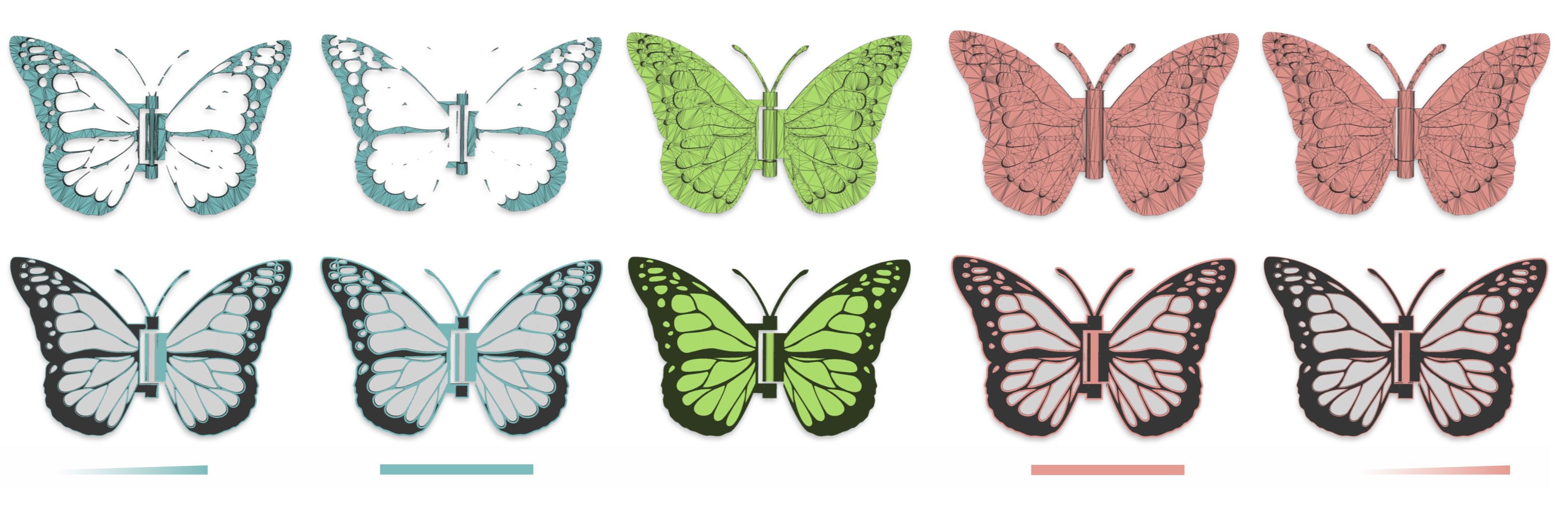
Figure 1. For a 3D mesh with arbitrarily complex geometry and topology, our approach can robustly produce its inward and outward offset surfaces, according to user desired either uniform or varying offset distances. We assign the non-uniform offset distance to each face of the input by linearly interpolating 0.001% and 0.5% of the diagonal length of the input’s bounding box. The top row shows the full views of the meshes and the bottom is their corresponding cut views.

1. Introduction

Offset mesh generation, which involves creating a parallel surface with a specific distance from a given shape, holds a place of critical importance in geometric modeling and mesh processing. This technique is fundamental in a variety of applications, including but not limited to computer-aided design and engineering, real-time rendering and animation, robotics, medical imaging, architectural design (Pham, 1992; Maekawa, 1999a). For example, it is instrumental for designing mechanical parts with specific thickness requirements, such as gears and casings. In the world of animation and 3D modeling, offset surfaces enable the creation of intricate and realistic characters and environments, providing the necessary depth and complexity.

Many prior works are proposed to generate offset surfaces for input meshes, such as explicit offsetting following normal directions (Jung et al., 2004), implicit distance function based iso-surfacing (Chen et al., 2023; Zint et al., 2023), Minkowski Sum based boolean approach (Hachenberger, 2009), and offsetting by ray-reps based method (Chen et al., 2019b). However, differently from the well-studied curve offset research in 2D (Tiller and Hanson, 1984; Vatti, 1992; Park and Chung, 2003) that have robust solutions for both constant radius and mitered offsets (see the inset), to the best of our knowledge, none of existing approaches in 3D can generate offset meshes in the mitered manner. Moreover, the methods for even constant radius offset typically suffer one or more of the following critical issues that hinder their practical usage: 1) lack of robustness in dealing with “dirty” data that may have open boundaries, non-manifold vertices and edges, and self-intersections, which is common in scanned or man-made models; 2) struggle to maintain the fidelity of the original shape, especially in handling complex geometries with sharp edges and intricate details, resulting in undesired artifacts in the offset surface; 3) computational inefficiency when the offset distance is small, which can often jointly pose memory issues. These issues collectively underscore the need for an innovative solution that can address the complexities of modern geometric shapes while ensuring computational efficiency and geometry fidelity.

In this work, we propose a new explicit surface offset generation method that can address the aforementioned issues. The robustness of our approach lies in that we make no assumptions of the input mesh, such as its manifoldness, watertightness, absence of self-intersections and degeneracies, etc, reformulating the offset meshing problem and algorithm design accordingly. We further employ exact algorithmic for robust geometric computations. The feature preservation is ensured through first redefining the offset distance from traditionally employed point-to-point to point-to-plane, and then generating the offset surface geometry that can capture sharp features by solving local quadratic energies and dynamic programming. While employing the rational number representation for exact computations, we strive to be efficient by designing several acceleration strategies including parallelization through spatial domain decomposition and dynamic programming for early rejection of the expensive intersection computations.

Our solution has the additional advantages over existing approaches: 1) the resulting offset mesh is similar with the input, from both the number of triangles and connectivity aspects; 2) we support variable offset distances over different surface regions, enabling broader applications than conventional offset methods.

We empirically compare our approach against state-of-the-arts on a subset of the Thingi10K dataset (Zhou and Jacobson, 2016). Our method exhibits a significant improvement in terms of feature preservation, robustness, and element count at the same time. All the data shown in the paper can be found in the attached material, including a video to show their visual quality.

2. Related Work

We briefly review prominent methods related to offset meshing, which are based on direct offsetting, distance field, Minkowski sum, medial axis and skeleton, and ray casting.

Direct Offsetting

A prominent method proposed by (Jung et al., 2004) offsets based on vertex normal direction. Although efficient, it struggles with holes in complex CAD models, leading to offset meshes that can be defective, particularly in scenarios involving self-intersections. The precision issues arising from floating-point operations in self-intersections have been addressed using infinite precision operations (Campen and Kobbelt, 2010), but results occasionally produce twisted meshes. Offsetting surfaces with polynomials or B-splines is explored in (Maekawa, 1999b). However, subsequent intersection operations are intricate. Another approach calculates offset positions based on distance and uniform distribution, followed by point cloud reconstruction (Meng et al., 2018).

Distance Field

These methods are popular in modern 3D printing (Brunton and Rmaileh, 2021). Generally, they require resampling to generate the final mesh, which can compromise geometric features, especially in detailed meshes (Wang and Chen, 2013). Challenges also arise from the grid density, preservation of sharp features, and computational efficiency. Some attempts, such as (Kobbelt et al., 2001), have tackled the ambiguity of the Dual Contouring and Marching Cube, but they tend to excel mostly with CAD models. In the study by (Liu and Wang, 2010), there are some improvements in computational efficiency. The method introduced in (Pavić and Kobbelt, 2008) tries to preserve sharp features, but it involves high grid density and computational expenses. An Octree-based method is proposed in the study by (Zint et al., 2023), which requires the input to be degenerate-free and may output offsets with self-intersections. While the feature-preserving approach introduced in (Chen et al., 2023) ensures nice geometry and topology properties of iso-surfaces, it cannot handle offset distances smaller than the grid size which is a common shortcoming shared all distance field based offset extraction methods.

Among the vast offset generation literature, we realize only one work (Chen et al., 2019a) tried to address the non-uniform offset problem based on dual-contouring (Ju et al., 2002). However, the approach would require an impractical grid resolution at regions with a small offset distance for tolerable offset reconstruction. More importantly, without much details of how the interpolation is performed for different offset distances within a grid cell, we infer that it either is computationally expensive for proper in/out sign determinations, or has discontinuity issues leading to bumpy artifacts. Moreover, their generated offset meshes would often have self-intersections, even if the input is both topologically simple and geometrically high quality.

Minkowski Sum Method

The Minkowski sum offers a solution for mesh offsetting by calculating the sum of mesh and sphere polygons (Rossignac and Requicha, 1986). An advanced method in (Hachenberger, 2009) computes the exact 3D Minkowski sum of non-convex polyhedra by decomposing them into convex parts. Despite its robustness (Project, 2023), the method is slow for complex CAD models and struggles with variable thickness offsets and sharp feature preservation.

Skeleton-Based Methods

Skeletal meshes are prevalent in geometry processing (Tagliasacchi et al., 2016). The mesh model can be represented by medial axes and spheres (Amenta et al., 2001; Sun et al., 2015). There are techniques to generate skeleton meshes (Lam et al., 1992; Li et al., 2015). However, they usually cannot handle general models with open boundaries, self-intersections, etc. There have been efforts to simplify medial axes (Sun et al., 2013). Offsetting can be achieved by adjusting the radius of the balls on the skeleton. Still, these methods often fall short with models with sharp features.

Ray-Based Methods

This approach (Chen et al., 2019b; Wang and Manocha, 2013) is rooted in the dexel buffer structure (Van Hook, 1986). A recent algorithm in (Chen et al., 2019b) offers an efficient parallelized method using rays and voxels to compute mesh offsets, bypassing the need for distance field computation. Nonetheless, due to the grid’s voxel-like structure, a high density is essential for accurate shape representation, leading to increased computational costs and dense mesh outputs. The approach also mainly considers a consistent offset, further steps have to be designed for the mesh representation conversion.

3. Method

In this section, we provide our problem statement, give the pipeline overview, explain each step in detail, and introduce the performance improvement strategies.

Problem Statement:

The input of our approach contains a 3D triangle mesh $M_{\text{I}}$ with an arbitrary geometry and topology configuration, an integer variable $s\in\{-1,1\}$ to indicate the offsetting direction, and an offset scalar $d_{i}$ per $T_{i}$ of $M_{\text{I}}$ where $d_{i}$ could vary for different triangles. While locally to a triangle, $s=1$ means the offset direction has a positive product with the triangle’s normal and $s=-1$ is for the opposite direction, globally we employ the generalized winding number (Jacobson et al., 2013) for inward and outward checks to robustly handle $M_{\text{I}}$ with possibly gaps, duplicated elements, etc.

Our goal is to generate an offset mesh $M_{\text{O}}$ that satisfies three qualitative requirements. First, $M_{\text{O}}$ should have the offset distance to $M_{\text{I}}$ satisfying user desired value. Second, $M_{\text{O}}$ needs to have nice geometry and topology properties to enable the easy design of automatic downstream algorithms. Third, $M_{\text{O}}$ should contain as few as possible elements such as triangles, allowing efficient computations for the various applications of offset. While hard to properly perform a quantitative measure, we further require $M_{\text{O}}$ to capture the geometry feature of $M_{\text{I}}$ as much as possible, especially for prominent sharp features since we aim for reproducing the mitered offset effect.

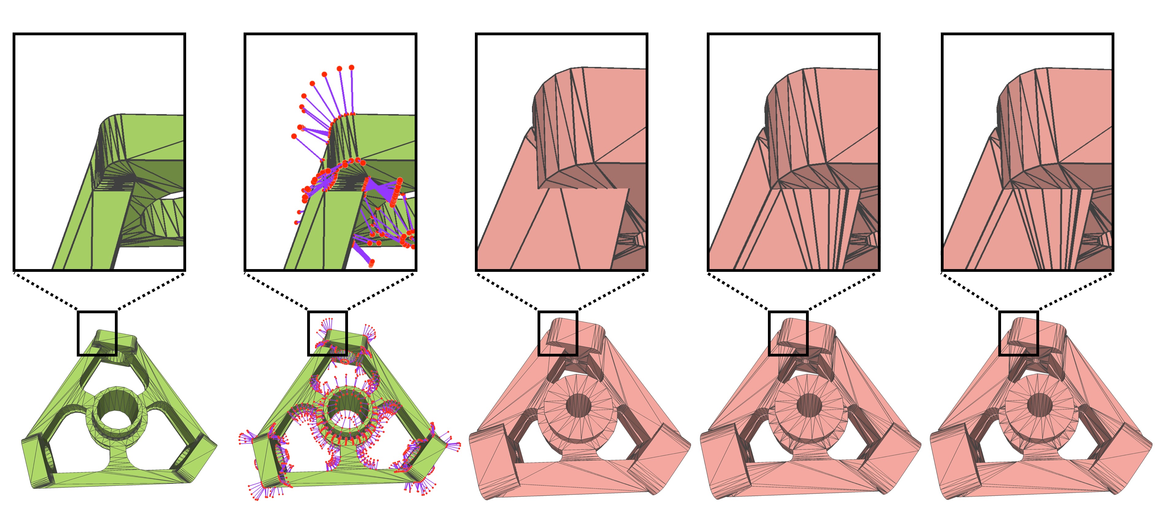
Figure 2. Pipeline : starting from a triangle mesh $M_{\text{I}}$ (left most), our approach first generates its vertices’ offset points (second to the left), then builds an offset polyhedron for each of its triangle, edge and vertex (middle). After that, we convert the polyhedra set to an intersection-free triangle soup $M_{\text{C}}$ by filtering out those triangles not part of $M_{\text{O}}$ (second to the right), Along with some acceleration measures, this approach involves selecting only a subset of triangles from the polyhedra set for computation, which may result in the creation of some holes. Finally, by detecting the boundaries of the holes, we retrieve the triangles that were excluded in the previous step, Then we construct the connectivity of $M_{\text{O}}$ (right).

Method Overview:

As illustrated by Fig. 2, we tackle the surface offset problem by first offsetting each vertex of $M_{\text{I}}$ to one or more corresponding points through the solving of a point-to-plane constrained quadratic energy (Section 3.1, Fig. 2 second to the left), and then constructing a polyhedron representing the local offset volume corresponding to each vertex, edge, and triangle of $M_{\text{I}}$ Section 3.2, Fig. 2 middle). Using a set of acceleration strategies, we then perform boolean operations of the offset volumes to obtain a triangle soup, $M_{\text{C}}$, representing the geometry of $M_{\text{O}}$ (Section 3.3, Fig. 2 second to the right), which are finally connected to complete the generation of user desired $M_{\text{O}}$ (Section 3.4, Fig. 2 right).

3.1. Vertex Offset

This step is to generate the offset points for each vertex $V_{i}\in M_{\text{I}}$. As illustrated in the inset, $V_{i}$ might correspond to one or more points depending on different local configurations, such as non-manifoldness, saddle region etc. For easy explanation, we first introduce the simple but effective linear constrained quadratic optimization solution when $V_{i}$ has only one offset point, and then

describe how to tackle the general scenario, i.e. multiple offset points, via dynamic programming.

linear constrained quadratic optimization

Let $O_{i}$ be $V_{i}$’s unique offset, we assume the local region of $V_{i}$ is formed by a triangle set $\mathcal{T}_{i}$ where every triangle $T_{j}\in\mathcal{T}_{i}$ is equipped with an offset distance $d_{j}$. Denote $N=|\mathcal{T}_{i}|$. Note that, since we assume the input could have an arbitrary topology, we set $\mathcal{T}_{i}$ to be the set of triangles that $V_{i}$ directly adjacent to if the boundary of this triangle set contains a simple circle topology. Otherwise, we consider $\mathcal{T}_{i}$ as the set of all triangles with an $\epsilon$ distance from $V_{i}$. We set $\epsilon=10^{-5}l$ by default, where $l$ is the length of the diagonal of $M_{\text{I}}$’s bounding box.

By requiring the point-to-plane distance from $O_{i}$ to $T_{j}\in\mathcal{T}_{i}$ to be $d_{j}$, we can compute $O_{i}$ by solving the following optimization:

(1) $$\underset{O_{i}}{\text{argmin}}\;||O_{i}-V_{i}||^{2}\quad\text{s.t.}\;\text{P}_{j}^{\text{T}}O_{i}=d_{j}\quad\forall j<N,$$

where $\text{P}_{j}=[a\text{ }b\text{ }c\text{ }d]^{\text{T}}$ represents the plane of triangle $T_{j}$ defined by the equation $ax+by+cz+d=0$ and $a^{2}+b^{2}+c^{2}=1$. The optimization term $||O_{i}-V_{i}||^{2}$ is introduced to pick the position of $O_{i}$ nearest to $V_{i}$ when the solution space is a plane or a line. While Equation 2 may be solved using OSQP solver (Stellato et al., 2020), due to numerical precision issues, we solve it as a two step process. We first solve an unconstrained quadratic problem:

(2) $$\underset{O_{i}}{\text{argmin}}\;\lambda||O_{i}-V_{i}||^{2}+\sum_{j}{(\text{P}_{j}{{}^{\text{T}}}O_{i}-d_{j})^{2}}\quad\forall j<N.$$

The role of $\lambda$ is to ensure that, in cases where there are infinitely many solutions satisfying the point-to-plane distances, an optimal solution can be selected, while minimizing its impact on other scenarios. Consequently, it is necessary to set it to a very small number. By default, we set $\lambda$ to $10^{-9}$. Subsequently, this expression can be solved using the least squares method. We employ the QR decomposition from the Eigen library for the solution.

We then perform a distance check for each plane to ensure $|\text{P}_{j}^{\text{T}}O_{i}-d_{j}|\leq\alpha$, where $\alpha$ is a parameter to control how much the user desired point to plane distance is satisfied. Due to the presence of $\lambda$, the distances between the solved point position and the planes will always be slightly off from the desired values. Therefore, $\alpha$ cannot be set to zero but must be assigned a small value. We set $\alpha=10^{-6}$ by default. Since there could be cases that cannot satisfy the distance check for all triangles in $\mathcal{T}_{i}$, we then propose to address this issue by generating multiple offsets for a vertex as detailed in the next paragraph.

Dynamic Programming

When there is no solution found for Equation 3, we compute multiple offset points. We propose to solve this issue by dividing the triangle set $\mathcal{T}_{i}$ into $K$ subsets, denoted by $\mathcal{Q}=\{\mathcal{T}_{i}^{0},\mathcal{T}_{i}^{1},\cdots\}$ where $|\mathcal{Q}|=K$, and we compute an offset point $O_{i}^{k}$ for each subset $\mathcal{T}_{i}^{k}$. Denote $\mathcal{R}$ as the offset point set, i.e. $\{O_{i}^{0},O_{i}^{1},\cdots\}$ and $|\mathcal{R}|=K$. Therefore, we need to solve the following problem:

(3) $$\begin{split}\underset{\mathcal{Q},\mathcal{R}}{\text{argmin}}\;&\lambda\sum_{k}||O_{i}^{k}-V_{i}||^{2}+\sum_{k}{(\text{P}_{j}^{k}{{}^{\text{T}}}O_{i}^{k}-d_{j}^{k})^{2}}\\ \end{split}$$

The challenge arises for deciding the $K$ subsets while ensuring the point-to-plane distance constraint for the planes of $\mathcal{T}_{i}^{k}$ for each $O_{i}^{k}$. While we can simply decompose $\mathcal{T}_{i}$ based on the similarity of the normal of the triangles, solution of $O_{i}^{k}$ is still not guaranteed to exist and normal could be wrongly computed when floating point precision is involved. Instead, we propose a dynamic programming strategy to solve $\mathcal{Q},\mathcal{R}$ as detailed below, where Algorithm 1 is the pseudo-code.

Given the $N$ triangles in $\mathcal{T}_{i}$, a subset could have $2^{N}$ possible configurations. We encode each subset using the binary representation with length $N$. For example, $0b010101$ represents the subset of $\{T_{0},T_{2},T_{4}\}$ for $N=6$, while $0b100100$ is the subset of $\{T_{2},T_{5}\}$. We use $D_{o}$ to store the energy values of Equation 2 when solving an offset vertex $O_{i}^{k}$ for the group of triangles $\mathcal{T}_{i}^{k}$ represented in the aforementioned binary format $x$, and $D_{c}$ to store the coordinates of the corresponding offset vertex $O_{i}^{k}$. As shown in Algorithm 1, we employ a recursive scheme (lines 2-12) to find the best group decomposition, where for each level of the recursion we decompose a set $x$ into two subsets $\tilde{x}$ and $x-\tilde{x}$ if $x$ cannot be solved by Equation 2. Here, the union of the triangles represented by $\tilde{x}$ and $x-\tilde{x}$ is the same as the triangle set of $x$. In this case, we use the an array of scalars, $D_{s}$, to record the best decomposition for $x$, i.e. $D_{s}[x]=\tilde{x}$. From which, we can retrieve all the decomposed subsets of $\mathcal{T}_{i}$, as shown by lines 15-20 of Algorithm 1. Note that, the dimension of $D_{o}$, $D_{c}$, and $D_{s}$ are all $2^{N}-1$.

The introduced dynamic programming has a computational complexity of $O(3^{k}+2(1-2^{k}))$ (Giraudo, 2015; A10, 2024). The computation is efficient for $N\leq 12$, e.g. $\leq 0.01s$ without any parallelization. Since the dynamic programming operates independently in each local context, it can be fully parallelized. However, if $N$ becomes excessively large, the computation time may grow significantly as show in Fig. LABEL:fig:speedforclassify.

To address this problem, we first classify the the planes defined by $\mathcal{T}_{i}$ into groups where the planes within a group have the similar normal. We then compute an averaged plane for each group and consider the averaged one as the plane for all the triangles with each group.

To summarize, we compute the offsets for each vertex of $M_{\text{I}}$ by firstly merging its adjacent triangles with similar normals, and then perform Algorithm 1 to solve the offset points. Fig. 4 illustrates different offset cases on a real example.

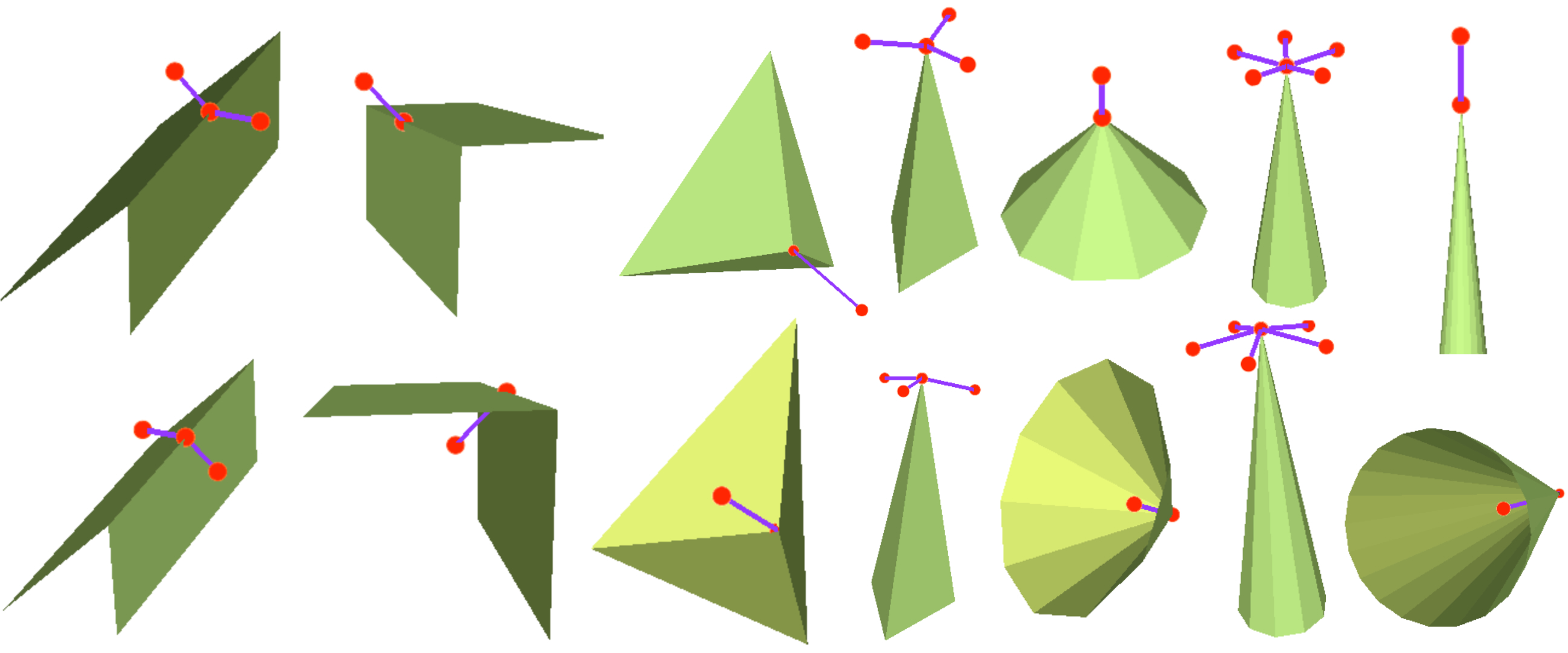
Figure 4. Nine different vertex offset scenarios computed by our approach on a mesh example. Each column corresponds to one scenario, where the top and bottom rows show two different offset direct (outward and inward). It can be observed that in some sharp cases, the points generated by the inward offset of vertices may appear outside the input model. This situation does not pose any issues. The subsequent convex hull and winding number computations will exclude these points and .

Input: $V_{i}$, $\mathcal{T}_{i}$, $d$, $T_{j}\in\mathcal{T}_{i}$

Output: $\mathcal{Q}$, $\mathcal{R}$

1 Set each entry of $D_{o}$, $D_{c}$, and $D_{s}$ as NULL

2 Function DFS(x):

3       if $D_{o}[x]\neq\text{NULL}$ then

4             return $D_{o}[x]$

5      $D_{o}[x]\leftarrow\infty$

6       if Eq.2($x$) is solvable then

7             Set Eq.2($x$)’s energy and solution to $D_{o}[x]$ and $D_{c}[x]$

8      for each $\tilde{x}$ derived from $x$ do

9             $o\leftarrow$ DFS($\tilde{x}$) + DFS($x-\tilde{x}$)

10             if $o<D_{o}[x]$ then

11                   $D_{o}[x]\leftarrow o$, $D_{s}[x]\leftarrow\tilde{x}$

12                  

13      return $D_{o}[x]$

14DFS($2^{N}-1$)

15 $\tilde{\mathcal{Q}}\leftarrow\emptyset$, $\mathcal{R}\leftarrow\emptyset$, $\tilde{\mathcal{Q}}.push(2^{N}-1)$

16 while $\tilde{\mathcal{Q}}\neq\emptyset$ do

17       $x\leftarrow\tilde{\mathcal{Q}}.front()$, $\tilde{\mathcal{Q}}.pop()$

18       if $D_{s}[x]=\text{NULL}$ then

19             $\mathcal{Q}.insert(x)$, $\mathcal{R}.insert(D_{c}[x])$

20            

21      else

22             $\tilde{\mathcal{Q}}.push(D_{s}[x])$, $\tilde{\mathcal{Q}}.push(x-D_{s}[x])$

23            

Algorithm 1 Dynamic Programming for Vertex Offset

3.2. Local Offset Polyhedron

After generating the offset points of $M_{\text{I}}$, this step is to generate the local offset volumes for the elements of $M_{\text{I}}$, i.e. vertices, edges, and triangles. Ideally, if there is only one offset point for each vertex, then we only need to generate the local offset volume $P_{i}$ for each triangle, $T_{i}\in M_{\text{I}}$, and $P_{i}$ is simply the triangle prism formed by $T_{i}$’s three vertices and their corresponding offset points as illustrated in Fig. 5 left.

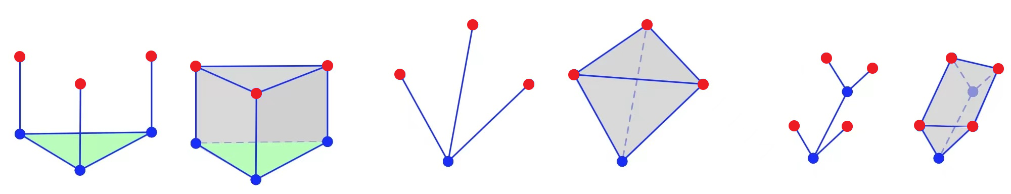
Figure 5. From left to right, the diagrams respectively illustrate the construction of offset volumes from a triangle, a vertex, and an edge.

In practice, however, one vertex may have multiple offset points, the offset volume computation for $M_{\text{I}}$ would be slightly involved. We tackle the problem by computing an offset polyhedron for each vertex, edge, and triangle of $M_{\text{I}}$ respectively. For each element, its offset polyhedron is computed as the convex hull of a point set associated with the element. To be specific, for a vertex $V_{i}$ of $M_{\text{I}}$, the point set includes $V_{i}$ and all its offset points $\{O_{i}^{0},O_{i}^{1},\cdots\}$ corresponding to the neighboring triangle set $\mathcal{T}_{i}$ (Fig. 5 middle). For an edge $E_{i}=\{V_{0},V_{1}\}$ of $M_{\text{I}}$, its polyhedron is computed as the following (Fig. 5 right). Assume $E_{i}$ is adjacent to a set of triangles $\mathcal{T}_{E_{i}}$, the point set of $E_{i}$ for the convex hull computation includes $V_{0},V_{1}$, and those from $V_{0}$’s and $V_{1}$’s offset points satisfying the following condition: the offset point’s corresponding triangle subset solved by Algorithm 1 contains any triangle of $\mathcal{T}_{E_{i}}$. Similarly, for a triangle $T_{i}=\{V_{0},V_{1},V_{2}\}$ of $M_{\text{I}}$, its polyhedron is the convex hull of the point set including $V_{0},V_{1},V_{2}$, and those offset points of $V_{0},V_{1},V_{2}$ as long as the offset point’s corresponding triangle subset solved by Algorithm 1 contains $T_{i}$.

This strategy leads to a set of polyhedra, denoted as $\mathcal{P}$, that their union forms the offset volume of $M_{\text{I}}$.

3.3. Geometry Extraction

After generating the offset polyhedra, this section is to compute all the triangles that constitute the geometry of $M_{\text{O}}$ in three steps.

First, we convert the all triangles from $\mathcal{P}$ into a conforming triangle mesh $M_{C}$ by resolving all the intersections, where the intersection points and line segments are taken as constraints for a subsequent Delaunay triangulation for each face of $P_{i}\in\mathcal{P}$. After this step, $M_{C}$ is intersection-free and contains only triangles. As illustrated in the inset, a triangle of $M_{C}$ can be classified into one of the five types, i.e. enclosed by a $P_{i}$ ($\text{T}_{\text{I}}$), shared by two $P_{i}$s that at different sides of the triangle ($\text{T}_{\text{II}}$), has an opposite sign to the offset direction as evaluated by $M_{\text{I}}$ ($\text{T}_{\text{III}}$), a triangle of $M_{\text{I}}$ ($\text{T}_{\text{IV}}$), and a face of $M_{\text{O}}$ ($\text{T}_{\text{V}}$). Since $\text{T}_{\text{IV}}$ faces are properly tracked from the beginning, our next two steps are to obtain the triangles with type $\text{T}_{\text{V}}$ by filtering out those triangles belonging to the first three types.

Second, we identify and discard triangles with $\text{T}_{\text{I}}$ and $\text{T}_{\text{II}}$ through rational number represented ray intersection checks where the rays are shot from the centers of these faces along their normal directions. Both types can be easily detected by checking if there are any intersections between the rays and other polyhedra other than the ones these faces belong to.

Third, we detect faces with $\text{T}_{\text{III}}$ through the generalized winding number (Jacobson et al., 2013). Since the winding number computation is not exact, when the offset distances $d$ are close to the numerical precision, $\text{T}_{\text{III}}$ faces may be wrongly labeled, resulting redundant faces in $M_{\text{O}}$. However, accordingly to our extensive experiments, we don’t observe such an issue for $d\geq 10^{-6}$ for both uniform and varying offsets. Note that, if the input mesh is watertight and free of self-intersections, $\text{T}_{\text{III}}$ faces can be filtered out completely by employing (Project, 2023).

3.4. Topology Construction

After obtaining $M_{\text{C}}$, i.e., the triangle soup composing the geometry of $M_{\text{O}}$, in this section, we accomplish the connectivity of $M_{\text{O}}$ to make it free of degenerates and intersections under exact number representations. $M_{\text{O}}$ is also watertight given that the input is watertight and self-intersection-free.

We execute three steps to convert $M_{\text{C}}$ to $M_{\text{O}}$. First, we merge the vertices with the same coordinates in rational numbers so that all triangles are connected but zero-area holes may still exist. Second, we perform a hole-filling to remove the zero-area gaps. Given a boundary loop, our hole-filling is done by inserting an edge at a time with two criteria: this edge has no intersection with any other triangles and the areas of the newly generated polygons are still zero, until the loop is fully triangulated. Third, we eliminate all degenerate elements generated during the hole-filling step through edge collapse and edge split without changing the geometry of $M_{\text{O}}$.

3.5. Speedup Strategies

We employ speedup strategies from different aspects to improve the performance of our approach as detailed below.

We use OpenMP to trivially parallelize the vertex offset generation (Section 3.1) and the triangle polyhedra construction (Section 3.2). Furthermore, we spatially partition the spatial domain, which is covered by the geometry formed by extending $M_{\text{I}}$ along three axes with the largest offset distance, into cubes. Each cube is associated with the list of triangles of $M_{\text{I}}$ that are either fully contained or have intersections with the cube. So the computational domain of $M_{\text{O}}$ is constrained within each cube. We apply this strategy for Section 3.3 and Section 3.4.

Data-structure-wise, we employ AABB-tree data-structure as much as possible for spatial search of vertex, face, and polyhedron elements, such as the $\mathcal{T}_{i}$ collection for $V_{i}$ in Section 3.1, the polyhedron neighborhood search during intersection resolving, the ray-intersection check and the winding number computation during invalid triangle filtering in Section 3.3.

Based on the performance statistics, we find that the most time-consuming part is during the intersection resolving in Section 3.3 where an extensive number of exact computations (Hachenberger et al., 2007) are involved. While all intersections among the faces of the polyhedra of $\mathcal{P}$ are resolved by splitting the faces into intersection-free triangles, many of the resulting triangles are not part of $M_{O}$. In another words, if the entire or the most region of a face will be discarded for computing $M_{O}$, then most of the computations for resolving the intersections with this face are wasted since most of the resulting triangles will be discarded as well. Based on the principal that postponing unnecessarily intersection computations as much as possible, we propose a speedup strategy of Section 3.3 with the pseudo-code given by Algorithm 2.

Assume $\mathcal{T}$ is the set of triangles of all polyhedra of $\mathcal{P}$ and $\mathcal{T}_{o}$ is the set of all triangles of $M_{O}$. We first subdivide $\mathcal{T}$ into two sets $\mathcal{T}_{cur}$ and $\mathcal{T}_{later}$ where they contains triangles with high and low chances to be part of $M_{\text{O}}$ respectively. As shown in lines 2-10 of Algorithm 2, as an initialization, $\mathcal{T}_{later}$ contains triangles with two scenarios that are both unlikely to be part of $M_{\text{O}}$: sharing a vertex with $M_{\text{I}}$ and is inside (outside) $M_{\text{I}}$ for $s=1$ ($s=-1$). We then obtain $\mathcal{T}_{o}$ in an iterative way by constructing the most of it using $\mathcal{T}_{cur}$ (lines 12-23) and gradually refining it using $\mathcal{T}_{later}$ (lines 11 and 24-29). By doing so, the output of Algorithm 2 is ensured to be same as the brute-force approach in Section 3.3. During the construction of $\mathcal{T}_{o}$ using $\mathcal{T}_{cur}$,

we identify a scenario that for a triangle of $\mathcal{T}_{cur}$ that intersects with many polyhedra, a large part of it may be covered by one or several of those polyhedra. For such faces, there would be many intersection computations to produce $\text{T}_{\text{I}}$ and $\text{T}_{\text{II}}$ sub-triangles that are eventually discarded through ray-casting test. The inset illustrates a simplified scenario in 2D. Accordingly, in lines 17-22 of Algorithm 2, we propose to subdivide $T_{i}$ into triangles by a subset of all its intersecting polyhedra to avoid unnecessarily more detailed intersection computations. Specifically, given a triangle $T_{i}$ that has intersections with $N_{p}\geq 5$ polyhedra denoted by the set $\mathcal{P}_{i}$, we first subdivde $T_{i}$ into four smaller triangles, i.e. $T^{j}_{i}$ with $j=\{0,1,2,3\}$, using the mid-point subdivision. For each $T^{j}_{i}$, we then find the polyhedron from $\mathcal{P}_{i}$ that contains $T^{j}_{i}$ the most by creating several sampling points within $T^{j}_{i}$ and checking the number of sampling points contained by the polyhedron. After that, corresponding to $T^{j}_{i}$, there will be four polyhedra identified, $P^{j}_{i}$ with $j=\{0,1,2,3\}$. We then perform the intersection resolving procedure in Section 3.3 for $T_{i}$ and these four polyhedra to obtain a set of subdivided triangle set of $\tilde{\mathcal{T}_{i}}$. After filtering out those triangles in $\tilde{\mathcal{T}_{i}}$ that are fully contained in any $P^{j}_{i}$, $\mathcal{T}_{cur}$ will be updated.

By experimenting on several models randomly chosen from our testing dataset, we find that the early filtering strategy helps our pipeline achieves $\sim$30x performance gain in large offset distance e.g. more than $1\%$.

Input: $\mathcal{T}$, $\mathcal{P}$

Output: $\mathcal{T}_{o}$

1 Set $\mathcal{T}_{cur}$, $\mathcal{T}_{later}$, and$\mathcal{T}_{o}$ as $\emptyset$

2 for each $T_{i}\in\mathcal{T}$ do

3       if $s=1$ and Winding_number(centroid($T_{i}$)) $>0.5$ then

4             $\mathcal{T}_{later}$.push($T_{i}$)

5            

6      else if $s=-1$ and Winding_number(centroid($T_{i}$)) $\leq 0.5$ then

7             $\mathcal{T}_{later}$.push($T_{i}$)

8            

9      else if ($T_{i}$) have a vertex on $M_{i}$ then

10             $\mathcal{T}_{later}$.push($T_{i}$)

11            

12      else

13             $\mathcal{T}_{cur}$.push($T_{i}$)

14            

15while $\mathcal{T}_{cur}\neq\emptyset$ do

16       $\mathcal{T}^{\prime}_{cur}\leftarrow\emptyset$

17       for $T_{i}\in\mathcal{T}_{cur}$ do

18             if $N_{p}<5$ then

19                   $\mathcal{T}^{\prime}_{cur}$.push($T_{i}$)

20                  

21            else

22                   Subdivide $T_{i}$ into $T^{0}_{i},T^{1}_{i},T^{2}_{i},T^{3}_{i}$

23                   Compute $P^{j}_{i}$ containing $T^{j}_{i}$ the most, $j=\{0,1,2,3\}$

24                   $\tilde{\mathcal{T}_{i}}\leftarrow$ resolving intersections between $T_{i}$ and $P^{0}_{i},P^{1}_{i},P^{2}_{i},P^{3}_{i}$

25                   for $t_{j}\in\tilde{\mathcal{T}_{i}}$ do

26                         if $t_{j}$ is not contained in $P^{0}_{i}||P^{1}_{i}||P^{2}_{i}||P^{3}_{i}$ then

27                               $\mathcal{T}^{\prime}_{cur}$.push($t_{j}$)

28                              

29      $\mathcal{T}_{o}\leftarrow$ perform Section 3.3 of $\mathcal{T}^{\prime}_{cur}$ and $\mathcal{P}$

30       $\mathcal{T}_{cur}\leftarrow\emptyset$

31       $\mathcal{B}\leftarrow$ Boundary of $\mathcal{T}_{o}$

32       for $T_{i}\in\mathcal{T}_{later}$ do

33             if $T_{i}$ intersects with $\mathcal{B}$ then

34                   $\mathcal{T}_{cur}$.push($T_{i}$)

35                   $\mathcal{T}_{later}$.delete($T_{i}$)

36                  

Algorithm 2 Speed up of Section 3.3

4. Experiments

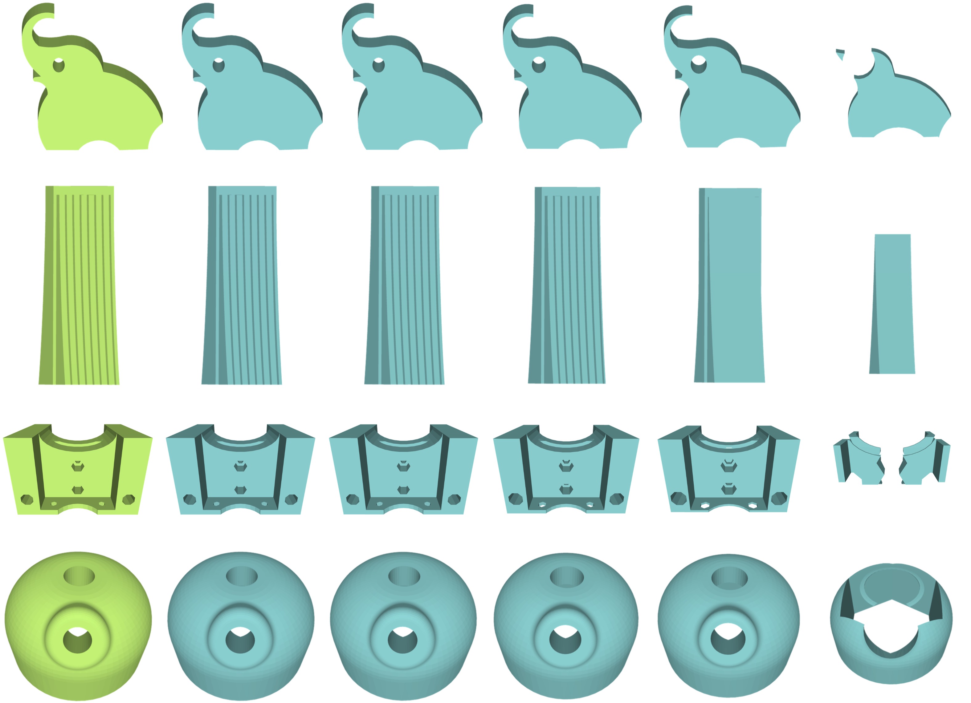
Figure 6. This figure shows the results of our algorithm for inward offsets at different distances. From left to right, the images are the input, $0.05\%l$, $0.1\%l$, $0.5\%l$, $1\%l$, and $5\%l$.

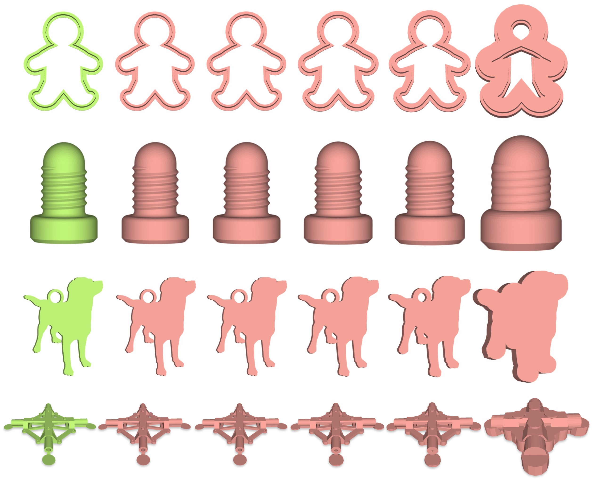
Figure 7. This figure shows the results of our algorithm for outward offsets at different distances. From left to right, the images are the input, $0.05\%l$, $0.1\%l$, $0.5\%l$, $1\%l$, and $5\%l$.

We run all our experiments on a desktop with a 10-cores Intel processor clocked at 5.30 Ghz and 32Gb of memory. We implement our approach in C++, with CGAL (Project, 2023) for exact computations. Throughout the entire paper, our offset distance parameter $d$ is formulated as the ratio of $l$ where $l$ is the length of the diagonal of the input’s bounding box, e.g. $d=1\%$ represents that the offset distance is actually $1\%l$. Please refer to the supplementary material for more information.

4.1. Dataset and Metrics

Dataset

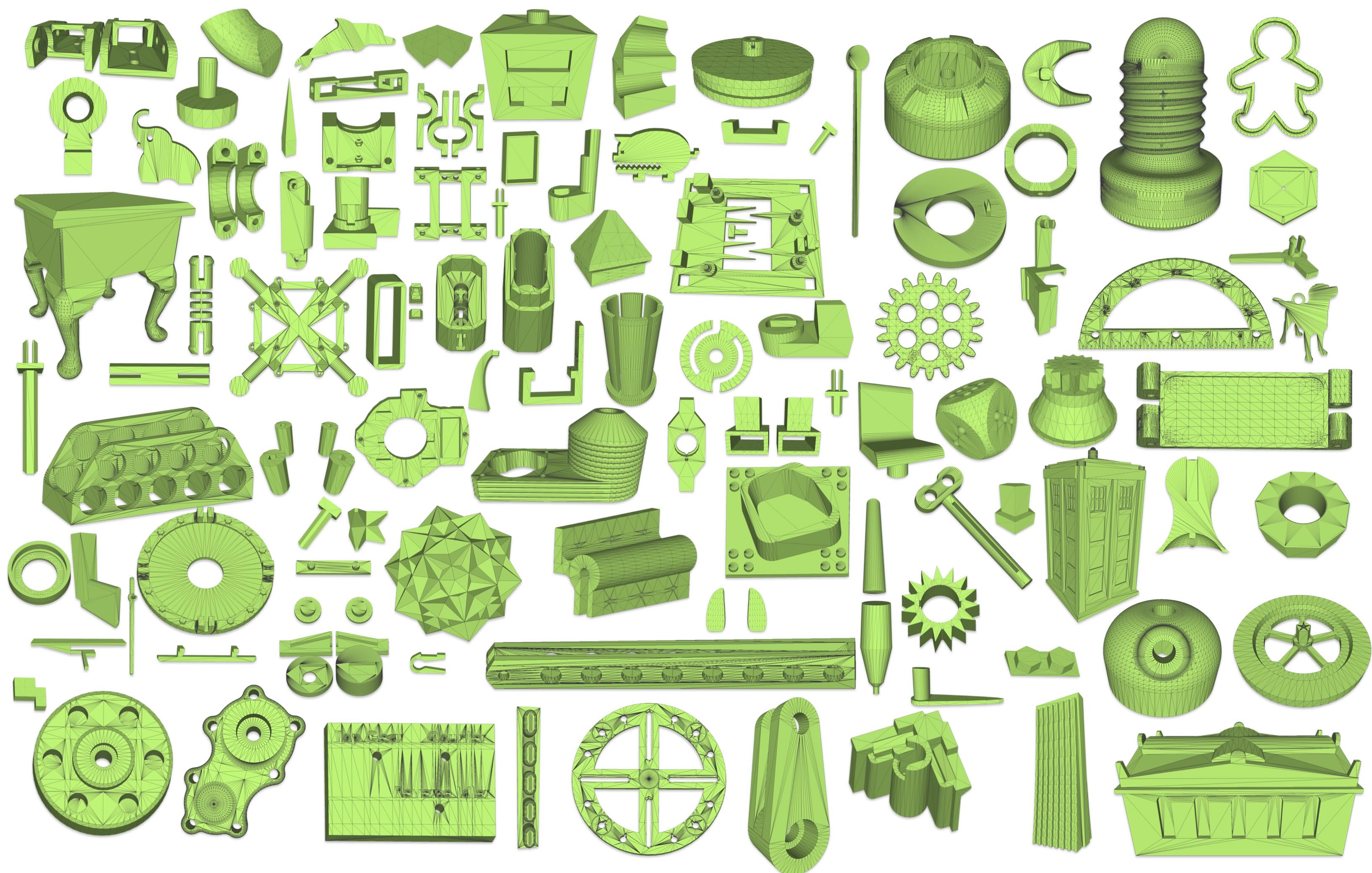
Figure 8. A visual gallery of the testing dataset.

We use 100 models chosen from Thingi10K (Zhou and Jacobson, 2016) as our test dataset as shown in Fig. 8. The dataset contains models with varying topology and geometry complexities, In the dataset, there are 50 models with fewer than 1000 triangles. There are 32 models with a triangle count ranging from 1000 to 5000. Additionally, there are 13 models with a triangle count between 5000 and 8000. Lastly, there are 5 models with more than 8000 triangles. 7 models are no manifold. 6 models are with open surface. The average number of genus, disconnected components intersecting triangle pairs and holes are 2.4, 1.94, 13.4 and 0.227, respectively.

For arbitrary input meshes, our generated offsets are guaranteed to be self-intersection-free and degenerate-free under exact representations. If the input mesh $M_{\text{I}}$ is watertight and self-intersection-free, our generated $M_{\text{O}}$ is guaranteed to be watertight.

We evaluate the geometry accuracy of our generated offset meshes by measuring how much of the distance between the offset mesh and input is different from the offset distance specified by users.

Mesh Distances

We employ the typically used point-to-point distance (Hausdorff distance) $H_{point}$ to measure the mesh distance between $M_{\text{O}}$ and $M_{\text{I}}$. Since we aim to generate mitered offset instead of the traditionally constant-radius offset, we also propose to measure point-to-plane distance $H_{plane}$ between $M_{\text{O}}$ and $M_{\text{I}}$.

Given a vertex $v$ and a triangle mesh $\tilde{M}$, we denote $d_{v}(v,\tilde{M})$ as the closest Euclidean distance from $v$ to $\tilde{M}$ and $\tilde{v}\in\tilde{M}$ is the point on $\tilde{M}$ closest to $v$. We further denote $d_{t}(v,\tilde{M})$ as the Euclidean distance from $v$ to the plane passing through $\tilde{v}$ and tangent to $\tilde{M}$. The computations of $H_{point}$ and $H_{plane}$ are summarized in Equation 4.

(4) $$\begin{split}H_{point}(M,\tilde{M})&\triangleq\frac{1}{|M|}\int_{M}d_{v}(v,\tilde{M})ds,\\ H_{plane}(M,\tilde{M})&\triangleq\frac{1}{|M|}\int_{M}d_{t}(v,\tilde{M})ds,\end{split}$$

$H_{point}(M_{\text{O}},M_{\text{I}})$ and $H_{plane}(M_{\text{O}},M_{\text{I}})$ measures the average distances from $M_{\text{O}}$ to $M_{\text{I}}$, while $H_{point}(M_{\text{I}},M_{\text{O}})$ and $H_{plane}(M_{\text{I}},M_{\text{O}})$ are from $M_{\text{I}}$ to $M_{\text{O}}$. The sampling strategy in Metro (Cignoni et al., 1998) is used for their computation. We use $D_{point}=|H_{point}-d|$ and $D_{plane}=|H_{plane}-d|$ to indicate how close of our generated mesh aligns with the user specified offset distance, where the smaller of $D_{point}$ and $D_{plane}$ the better.

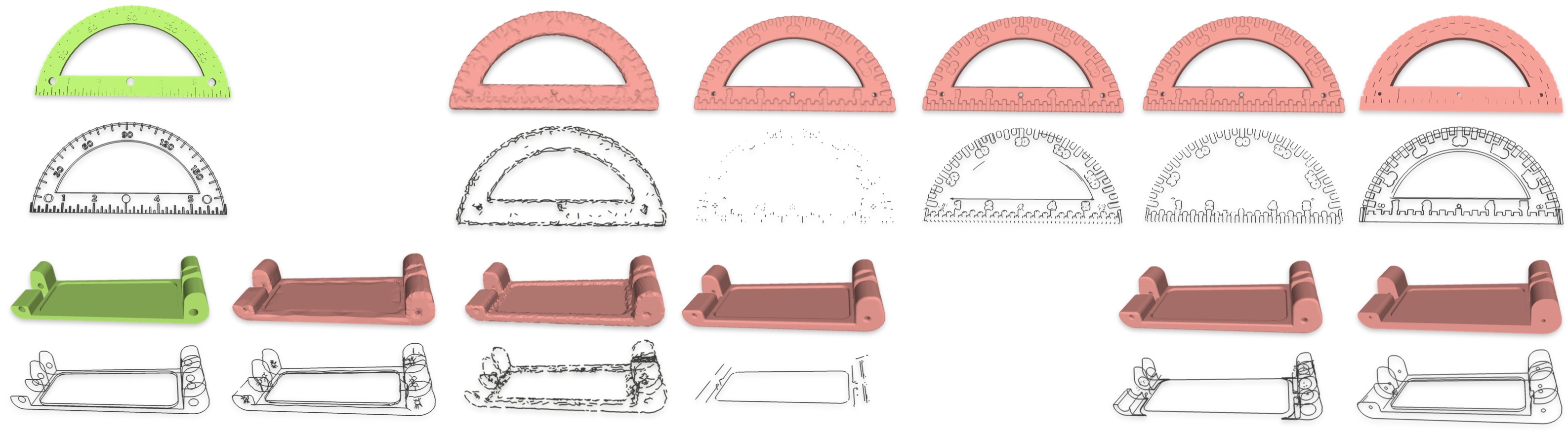
Figure 9. This figure shows an outward offset of $1\%l$. The left side is the input, and the back shows the comparison results of six methods. It can be seen that our method performs better in restoring feature lines.

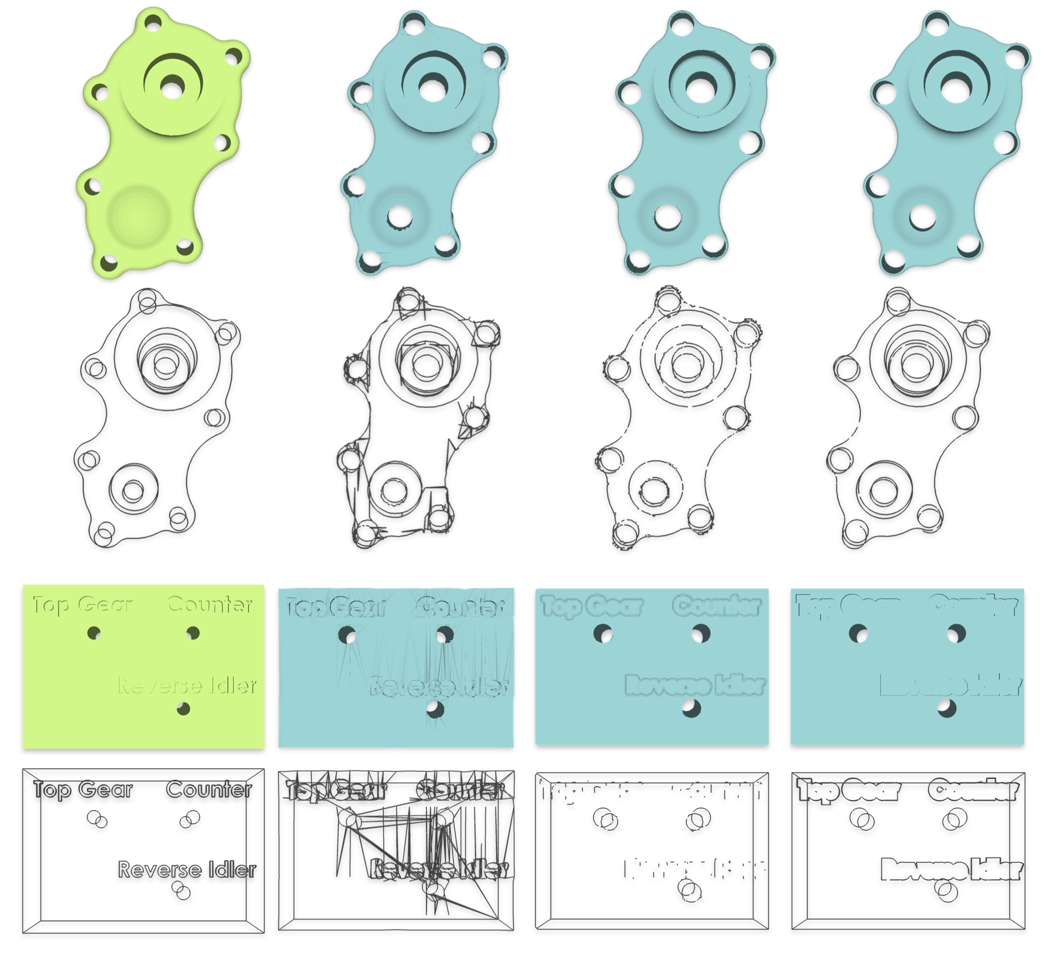
Figure 10. This figure shows an inward offset of $1\%l$. The left side is the input, and the back shows the comparison results of three methods. It can be seen that our method performs better in restoring feature lines.

Feature Preservation

Moreover, to quantitatively measure the effectiveness of various approaches in feature preservation, we propose to compute the difference between sharp features of the input and output meshes. Specifically, based on the simple angle thresholding strategy (Gao et al., 2019), we first detect feature lines $S_{M_{\text{I}}}$ and $S_{M_{\text{O}}}$ of $M_{\text{I}}$ and $M_{\text{O}}$ respectively (black lines shown in Fig. 9 and Fig. 10), then we uniformly sample $S_{M_{\text{I}}}$ and $S_{M_{\text{O}}}$. For each sample $v\in S_{M_{\text{I}}}$, we can find a closest sample $\tilde{v}\in S_{M_{\text{O}}}$. We denote $d_{angle}(v,S_{M_{\text{O}}})$ as the $l_{2}$ norm of the dihedral angles of the edges where $v$ and $\tilde{v}$ belong to. The difference between $S_{M_{\text{I}}}$ and $S_{M_{\text{O}}}$ can be calculated by

(5) $$\begin{split}D_{angle}(S_{M_{\text{I}}},S_{M_{\text{O}}})\triangleq\frac{1}{|S_{M_{\text{I}}}|}\int_{S_{M_{\text{I}}}}d_{angle}(v,S_{M_{\text{O}}})dl,\\ D_{angle}(S_{M_{\text{O}}},S_{M_{\text{I}}})\triangleq\frac{1}{|S_{M_{\text{O}}}|}\int_{S_{M_{\text{O}}}}d_{angle}(\tilde{v},S_{M_{\text{I}}})dl,\end{split}$$

where $D_{angle}(S_{M_{\text{I}}},S_{M_{\text{O}}})$ and $D_{angle}(S_{M_{\text{O}}},S_{M_{\text{I}}})$ measure the average distances from $S_{M_{\text{I}}}$ to $S_{M_{\text{O}}}$ and from $S_{M_{\text{O}}}$ to $S_{M_{\text{I}}}$ respectively.

4.2. Our Results

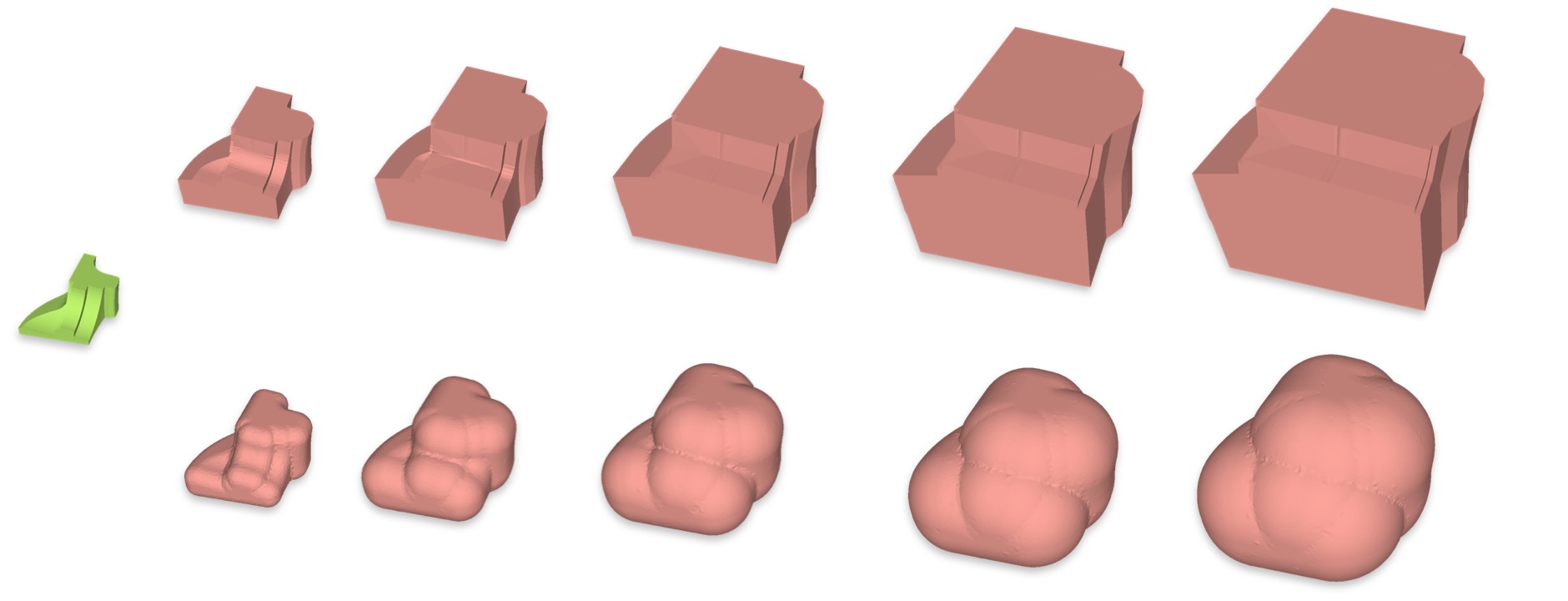
Figure 11. Display the large offset distance. It can be observed that generating an offset with a large offset distance using the original vertices may lead to creases due to the resolution limited by the number of vertices. The offset distance from left to right is $10\%l$, $20\%l$, $30\%l$, $40\%l$, $50\%l$ with outer direct. The first row is our method result, the second row is a case show radius based methods.

Our method requires only a single user-specified parameter, offset distance $d$, and generates the corresponding offset surface mesh that has the following unique properties.

Mitered offset

Aiming at generating the mitered offset surface, our approach provides the unique advantage over existing methods by respecting the features of the input excellently, as shown in Fig. 6, Fig. 7, Fig. 9, Fig. 10 and Fig. 17.

Unsurprisingly, as demonstrated in Fig. 11, as the offset distance gets larger, our generated surface tends to be a shape with a rectangular shape, distinct from the constant-radius offset with the tendency of being a sphere.

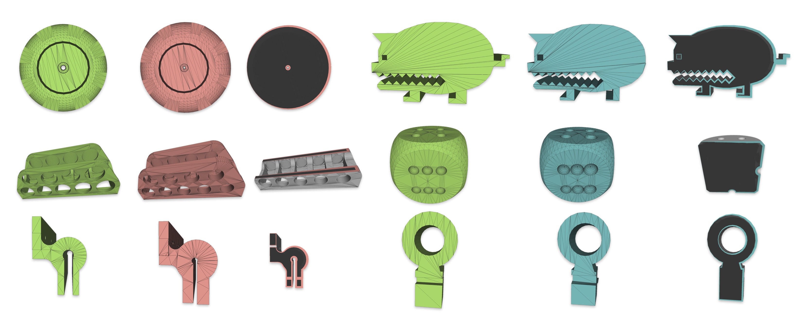
Figure 12. Our approach supports the generation of feature-preserving non-uniform offsets, i.e. from $0.01\%l$ to $2\%l$ for each model, for any given mesh inputs (green), either inwardly (cyan) or outwardly (red).

Non-uniform offset distance

By varying the offset distance $d$ for different triangles of the input, our approach can easily generate offset meshes with varying offset distances, as illustrated in Fig. 12 while maintaining the sharp features of the original meshes.

Topology

The topology of our generated mesh is similar to the input mesh, and the density of the mesh is close to or slightly greater than the input mesh as shown in Fig. LABEL:fig:denity.

Mesh Repair

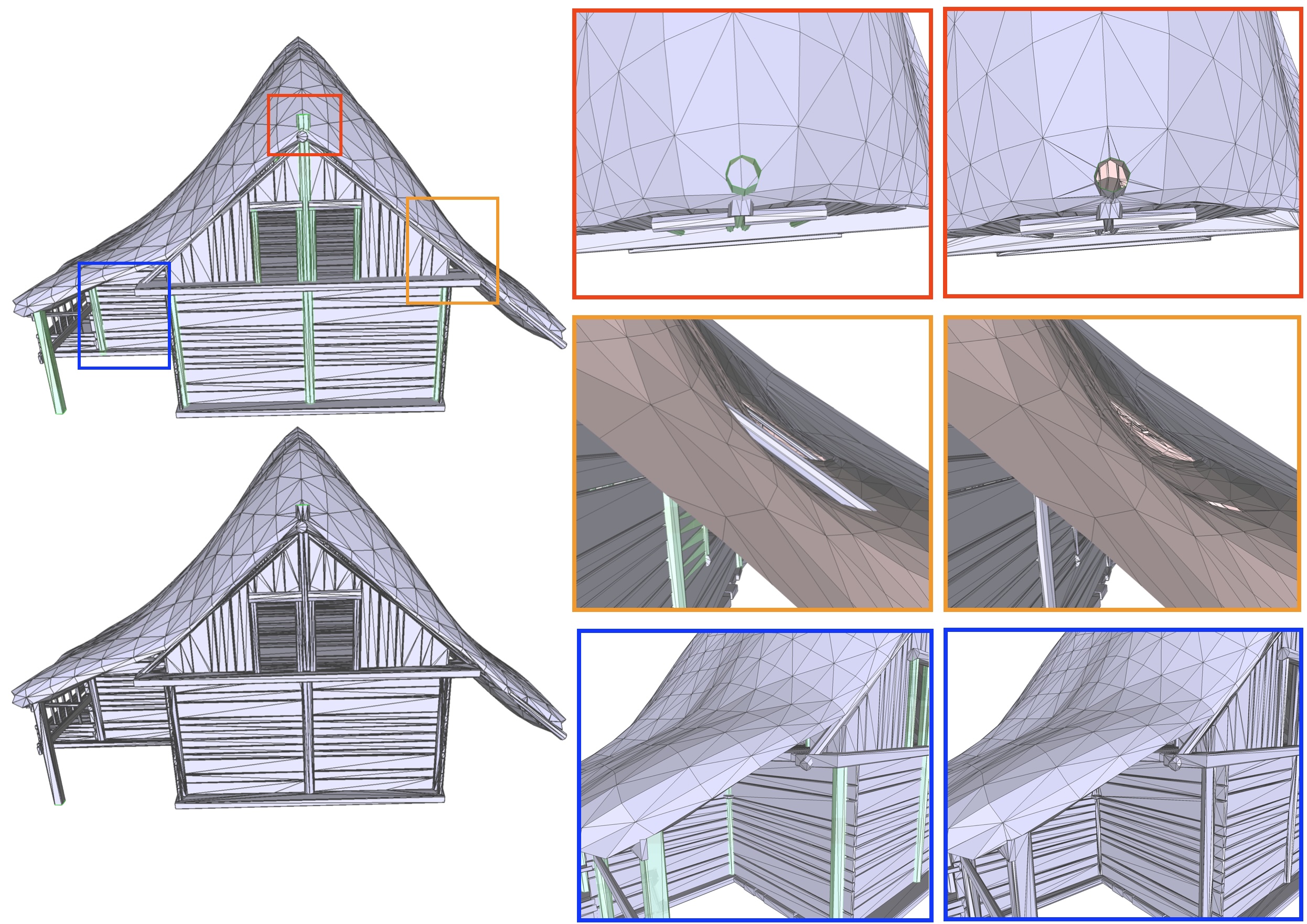
Figure 13. For damaged input models, when the normal vectors are correct, the outward offset with $0.1\%l$ can correct the mesh’s minor gaps, self-intersections, and internal redundant faces. Green triangles indicate the border on the mesh. The red box show the fix of delete the error facet, because of the limitation of resolution with figure the boundary triangle mark with green is not obviously, this triangle only have the width of the offset distance. The input mesh has 6170 points, 9991 faces, 416 disconnected components, and 17808 pairs of self-intersecting faces. 10.8 percent of the triangles are located on the boundary of the mesh. After performing offset calculations, the mesh has 20247 points, 41663 faces, and 6 disconnected components. After checking under rational numbers, 0 pairs of self-intersecting faces were found. After saving as an OBJ file with six significant digits for floating-point numbers and reopening it for checking, 947 pairs of self-intersecting faces were found, with 0.7 percent of the triangles located on the mesh boundary.

Our approach can perform mesh repairs if the input mesh contains small gaps, self-intersections and internal redundant faces, etc. Fig. 13 demonstrates the repair capability of our approach on such a case. Since our approach works nicely for small offset distances, it’s particularly beneficial for repairing meshes while introducing minor changes to the original mesh.

4.3. Comparisons

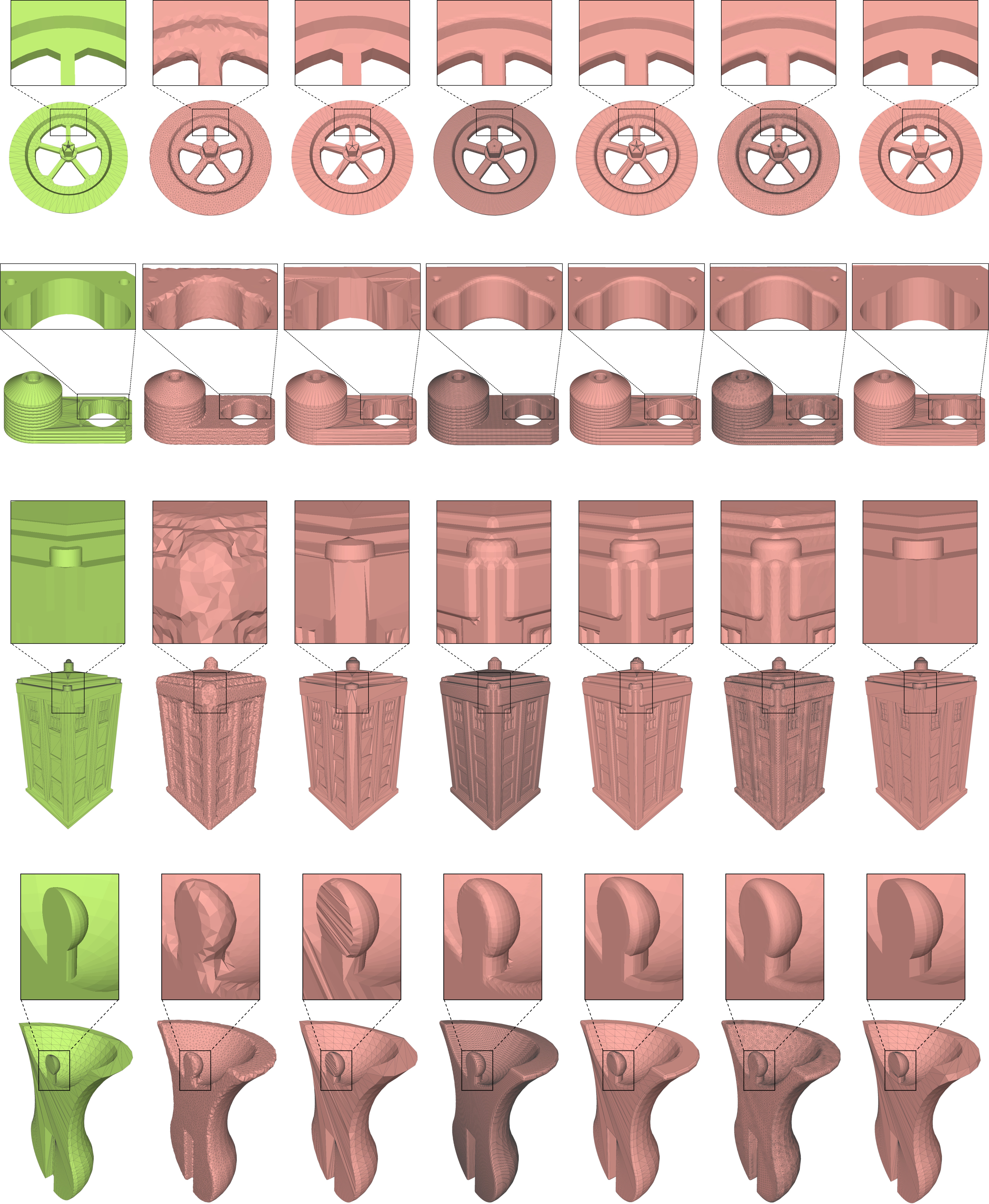
Figure 14. This figure shows a comparison of our method with other methods for outward offsets. It is clearly visible that our method has an advantage in restoring sharp features and achieves better detail restoration. The two value recorded in each sub-figure are generating facets number and running time.

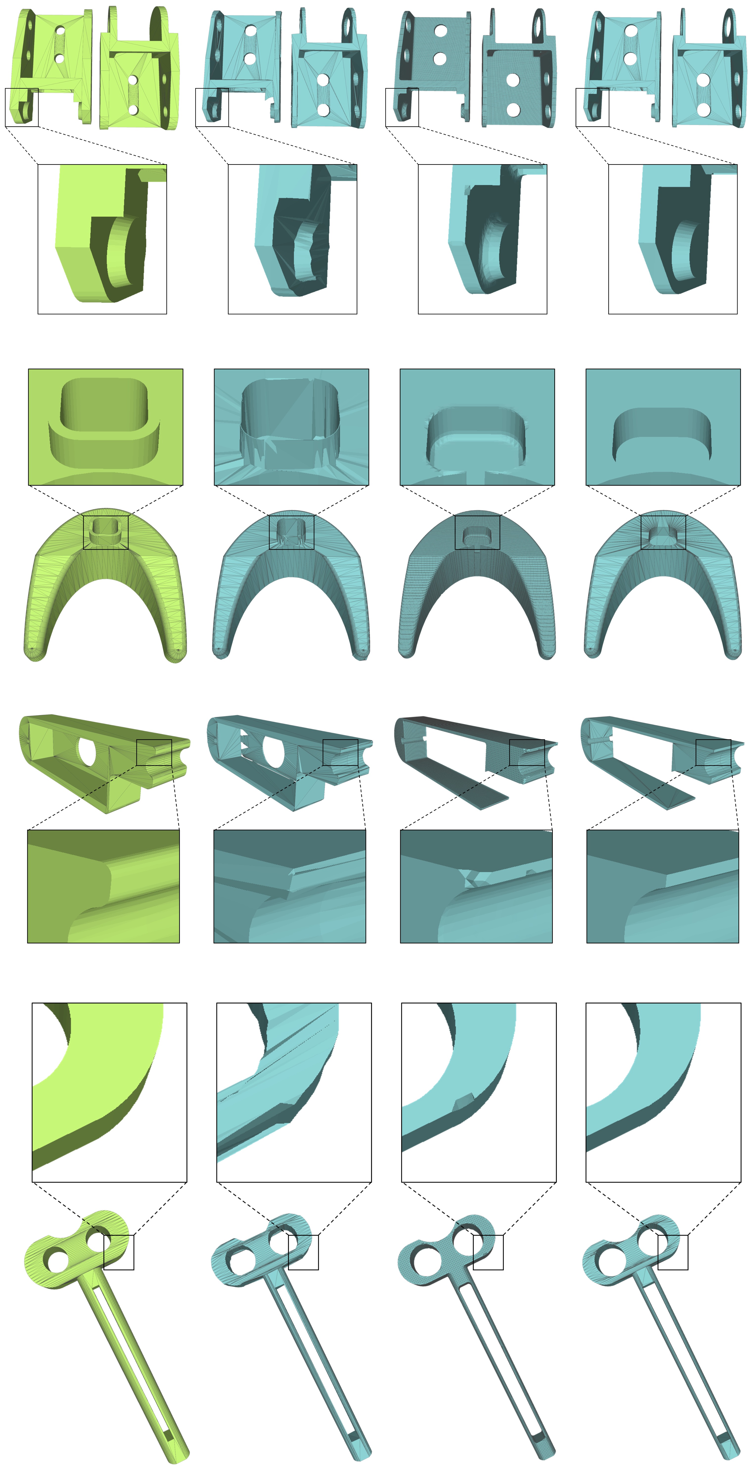
Figure 15. This figure shows a comparison of our method with other methods for inward offsets. It is clearly visible that our method has an advantage in restoring sharp features and achieves better detail restoration. And (Jung et al., 2004) can cause the error facet like show in the third row. The two value recorded in each sub-figure are generating facets number and running time.

Figure 16. From left to right, the figures represent the input, the output of our method after a 5%l offset, and the output of (Alpha Wrap 2022). The $D_{plane}(M_{\text{I}},M_{\text{O}})$ from the red point on the left model to the red point on the middle model is not as close to 5%l as the $D_{plane}(M_{\text{I}},M_{\text{O}})$ from the left model to the right model.

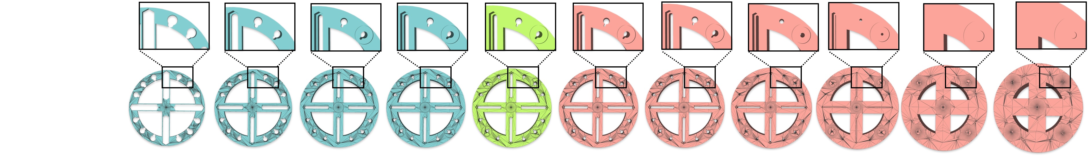
Figure 17. show the mesh in different offset to generate a empty mesh.

d	s	method	$D_{plane}({M_{o},M_{i}})$	$D_{point}({M_{o},M_{i}})$	$D_{angle}({M_{o},M_{i}})$	$D_{plane}({M_{i},M_{o}})$	$D_{point}({M_{i},M_{o}})$	$D_{angle}({M_{i},M_{o}})$	SUC	FACE	TIME
$0.05\%l$	-1	(Jung et al., 2004)	0.000132	0.000127	1.54531	N/A	N/A	2.18058	95	1938.6	281.5
		(Chen et al., 2023)	-	-	-	N/A	N/A	-	0	-	-
		Ours	0.000002	0.000006	0.193007	N/A	N/A	0.654405	100	2333.2	8.6
$0.1\%l$	-1	(Jung et al., 2004)	0.000265	0.000255	2.53419	N/A	N/A	3.4676	95	1955.3	203.9
		(Chen et al., 2023)	-	-	-	N/A	N/A	-	0	-	-
		Ours	0.000005	0.000012	0.265377	N/A	N/A	0.68033	100	2344.6	7.4
$0.5\%l$	-1	(Jung et al., 2004)	0.001382	0.001318	7.95833	N/A	N/A	9.77958	94	2010.2	235.4
		(Chen et al., 2023)	0.000055	0.000011	2.89306	N/A	N/A	2.64754	93	643734	70.4
		Ours	0.000052	0.000061	0.905081	N/A	N/A	1.51099	100	2576.2	15.6
$1\%l$	-1	(Jung et al., 2004)	0.003081	0.002937	12.3374	N/A	N/A	14.0914	88	1869.9	236.3
		(Chen et al., 2023)	0.000219	0.000029	5.84421	N/A	N/A	5.08535	100	172471	46.8
		Ours	0.000149	0.000116	2.10864	N/A	N/A	3.43261	100	2756	30.4
$5\%l$	-1	(Jung et al., 2004)	0.027254	0.026503	28.4349	N/A	N/A	24.1626	58	1238	539.9
		(Chen et al., 2023)	0.005515	0.000722	13.4986	N/A	N/A	12.2177	95	8459	1.5
		Ours	0.002249	0.000198	7.70095	N/A	N/A	7.84146	100	887	115.4
$0.05\%l$	1	$[$Alpha Wrap 2022$]$	0.000131	0.00016	9.70743	0.000117	0.000101	9.54859	100	21239	6
		(Jung et al., 2004)	0.000135	0.00013	1.35883	0.000296	0.000286	1.58863	95	1898.6	320.5
		(Chen et al., 2023)	-	-	-	-	-	-	0	-	-
		(Zint et al., 2023)	0.000419	0.00043	6.17889	0.001944	0.001733	6.00585	14	9334070	104.277
		$[$Minkowski sum 2023$]$	0.000711	0.000733	5.87534	0.000137	0.000151	5.83383	79	4967.2	425.1
		Ours	0.000001	0.000006	0.432793	0.000243	0.000239	0.868208	100	2314.1	6.6
$0.1\%l$	1	$[$Alpha Wrap 2022$]$	0.000098	0.000128	12.427	0.00038	0.000365	12.7267	100	17915.2	5.1
		(Jung et al., 2004)	0.000274	0.000267	2.19128	0.000616	0.000605	2.54556	93	1860.5	209.2
		(Chen et al., 2023)	-	-	-	-	-	-	0	-	-
		(Zint et al., 2023)	0.000132	0.000147	2.54262	0.001364	0.001165	4.16945	38	706214	247.291
		$[$Minkowski sum 2023$]$	0.000388	0.000413	6.30141	0.00029	0.000281	6.44548	79	4965.8	404.5
		Ours	0.000002	0.000007	0.474414	0.000495	0.000488	0.94634	100	2329.3	6.6
$0.5\%l$	1	$[$Alpha Wrap 2022$]$	0.000179	0.000074	20.6634	0.002488	0.002444	20.8965	100	15416	4
		(Jung et al., 2004)	0.001429	0.001351	6.43899	0.003207	0.003171	6.93395	88	1734.9	294.8
		(Chen et al., 2023)	0.000137	0.00001	6.73193	0.002582	0.002547	4.12022	90	570871	82.6
		(Zint et al., 2023)	0.000159	0.00004	2.19956	0.003191	0.003152	3.75481	77	180346	176.7
		$[$Minkowski sum 2023$]$	0.000346	0.00022	6.80817	0.002668	0.002638	6.97272	79	4858.7	422.9
		Ours	0.000119	0.000054	1.11749	0.0026	0.002565	1.52496	100	2562.3	15.2
$1\%l$	1	$[$Alpha Wrap 2022$]$	0.000575	0.000116	22.9292	0.005089	0.004997	21.6803	100	15900.4	3.4
		(Jung et al., 2004)	0.002953	0.002674	9.54129	0.006582	0.006485	9.971	86	1761	438.2
		(Chen et al., 2023)	0.000529	0.000037	8.53625	0.005337	0.005237	6.42665	100	126664	50.3
		(Zint et al., 2023)	0.000427	0.000023	4.7115	0.006542	0.006432	6.10771	94	112318	160.5
		$[$Minkowski sum 2023$]$	0.000948	0.000476	7.85758	0.005553	0.005463	7.55089	79	4639.1	403.3
		Ours	0.000303	0.000202	1.33165	0.005403	0.005302	1.79176	100	2950.9	42.8
$5\%l$	1	$[$Alpha Wrap 2022$]$	0.007818	0.000074	19.9315	0.029172	0.028471	18.6799	100	20533.5	2.7
		(Jung et al., 2004)	0.017843	0.013372	18.7543	0.037292	0.036438	18.0737	60	1319.8	780
		(Chen et al., 2023)	0.008097	0.000626	14.0047	0.029311	0.028586	13.6277	100	4862.7	1.5
		(Zint et al., 2023)	0.007315	0.000259	13.8445	0.03167	0.030529	13.8605	97	11977.9	45.6
		$[$Minkowski sum 2023$]$	0.009682	0.002429	14.7866	0.030825	0.029757	13.5377	79	3301.1	418.7
		Ours	0.006067	0.003044	5.09495	0.030913	0.02971	5.11666	94	3062.4	266.1

Table 1. This table displays the distance metrics and angle metrics for all methods. To ensure fairness, if a method cannot complete the generation of half of the models in the dataset within the constrained time at a certain offset distance, we will not evaluate it. It can be observed that our method tends to satisfy the point-to-plane distance more compared to the Hausdorff distance. Moreover, methods that generate a larger number of faces have an advantage in satisfying the Hausdorff distance. The column of angle means the different dihedral angle of sampling points in feature line. It can be easy to see our method have a good performance in maintain feature. The last three columns display the number of models successfully completed by all methods (denoted as SUC), the number of faces generated (denoted as FACE), and the average time consumed (denoted as TIME). The time cost of six timeout model of ours are $3602.65s,40004.5s,5539.63s,4476.96s,13355.2s,3679.04s$.

To demonstrate the robustness and effectiveness of our approach, we compare against five state-of-the-art competing approaches, i.e. (Alpha Wrap 2022), (Chen et al., 2023), [Minkowski sum 2023], (Zint et al., 2023), and (Jung et al., 2004), by batch processing the entire test dataset with varying offset distance settings, i.e. $d=0.05\%l$, $d=0.1\%l$, $d=0.5\%l$, $d=1\%l$ and $d=5\%l$ both inwardly (s = -1) and outwardly (s = 1). For outward offset, we compute the two way distances $H_{point}(M_{\text{O}},M_{\text{I}})$, $H_{point}(M_{\text{I}},M_{\text{O}})$, $H_{plane}(M_{\text{O}},M_{\text{I}})$, $H_{plane}(M_{\text{I}},M_{\text{O}}))$, $D_{angle}(S_{M_{\text{O}}},S_{M_{\text{I}}})$, and $D_{angle}(S_{M_{\text{I}}},S_{M_{\text{O}}})$. However, for the inward offset surface, we evaluate the single way distance only, i.e. $H_{point}(M_{\text{O}},M_{\text{I}})$, $H_{plane}(M_{\text{O}},M_{\text{I}})$, and $D_{angle}(S_{M_{\text{O}}},S_{M_{\text{I}}})$. The reason is that the inward offset surface may diminish as the offset distance gets large, as shown in Fig. 17, which renders the computed distances of $H_{point}(M_{\text{I}},M_{\text{O}})$, $H_{plane}(M_{\text{I}},M_{\text{O}})$, and $D_{angle}(S_{M_{\text{I}}},S_{M_{\text{O}}})$ not necessarily meaningful. We set a maximum execution time of one hour for each algorithm on each model. For processing time more than an hour, we automatically terminate the process and mark it as a failure. While we elaborate the detailed comparisons below, Fig. 9 and Fig. 14 show visual comparisons for outward offset results generated by the various methods, Fig. 10 and Fig. 15 illustrate the visual differences for inward offset meshes produced by the comparing approaches, and Table 1 demonstrates all the quantitative statistics.

(Alpha Wrap 2022) can robustly generate a watertight and orientable surface triangle mesh from an arbitrary 3D geometry input, but cannot compute inward offsets. Therefore, as shown in Table 1, we compare with it for cases only when $s=1$. It has two parameters, i.e. an alpha to determine the size of untraversable cavities when refining and carving a 3D Delaunay triangulation and an offset distance to control how far of the output mesh vertices from the input. We compare our algorithm with (Alpha Wrap 2022)’s CGAL implementation, set its offset distance using $d$. Its alpha parameter plays a critical role in determining the output mesh’s geometry approximation of the input and the approach’s computational speed. Using the same setting in the experiment section of (Alpha Wrap 2022), we set alpha = 100 for all the test in this paper. For the point-to-point distance $D_{point}$, while (Alpha Wrap 2022) performs excellently when measuring the distance from $M_{\text{I}}$ to $M_{\text{O}}$, as shown in the $D_{point}(M_{\text{I}},M_{\text{O}})$ column of Table 1, our approach has generally better accuracy when computing the distance from $M_{\text{O}}$ to $M_{\text{I}}$. Similar pattern happens for the point-to-plane distance $D_{plane}$ that our approach consistently achieves the smallest error for $D_{plane}(M_{\text{O}},M_{\text{I}})$ for all the offset distances, but (Alpha Wrap 2022) has the best accuracy for $D_{plane}(M_{\text{I}},M_{\text{O}})$. While this seems unexpected since $D_{plane}$ is designed for measuring the mitering offset distances, our approach may remove tiny dents as show in Fig. 16 that can lead to large $D_{plane}(M_{\text{I}},M_{\text{O}})$ and $D_{point}(M_{\text{I}},M_{\text{O}})$. In fact, our approach captures the sharp feature of the input excellently, achieving the best feature preservation among all the approaches for all the tested offset distances, as shown by the $D_{angle}(M_{\text{I}},M_{\text{O}})$ and $D_{angle}(M_{\text{O}},M_{\text{I}})$ columns of Table 1, and Fig. 9.

Comparison with (Chen et al., 2023)

We compare our algorithm with (Chen et al., 2023) by directly running their provided online executable program. While (Chen et al., 2023) can robustly handle general inputs, relying on voxel discretization of the unsigned distance function and maching-cube-like linear approximation of the iso-surface, (Chen et al., 2023) can generate results only when the discretization is coarse as shown by the $D_{point}(M_{\text{O}},M_{\text{I}})$ for $d=0.5\%l,s=-1$, $d=1\%l,s=-1$ and $d=0.5\%l,s=1$. However, the provided implementation would incur memory and computational issues for small offset distances, which is denoted as “$-$” in Table 1 for program crashes. Although introducing the feature preserving EMC33 scheme, their results tend to produce creases, leading to noisy feature curves as illustrated in Fig. 9 and Fig. 10.

Comparison with (Zint et al., 2023)

We compare our algorithm with (Zint et al., 2023) by running directly the source code provided by the authors. Their method also generates the mesh through implicit iso-surface extraction, similar to (Chen et al., 2023). By using octree, it can improve performance at small offset distances. The results of this algorithm are controlled by three main parameters: the minimum octree depth (d0), the maximum octree depth (d1), and the octree depth for resolving non-manifold vertices (d2). We use the default setting, i.e. d0 = 0, d1 = 10, and d2 = 12. Due to the usage of dual contouring for iso-surface extraction, this approach preserves feature lines very well, only second to our algorithm as show in the $D_{angle}(M_{\text{I}},M_{\text{O}})$ and $D_{angle}(M_{\text{O}},M_{\text{I}})$ columns of Table 1 and as show in Fig. 9. It can get the best or close to the best result in $D_{point}(M_{\text{O}},M_{\text{I}})$ metric. For all the tested offset distances, (Zint et al., 2023) produces results with consistently large dense meshes as compared to most of the other approaches. Especially as the offset distance gets small, the face numbers of $M_{\text{O}}$ can reach to millions of triangles, e.g. over 9M for $d=0.05\%l$. Furthermore, their provided program never successfully processes the entire dataset for the different batch tests. Due to unknown issues, the code provided by (Zint et al., 2023) cannot handle inward offsets, therefore, we only perform the outward offset experiments.

Comparison with [Minkowski sum 2023]

This method employs the computational results of the Minkowski sum of a sphere (represented as a polyhedron) and $M_{i}$. It has a corresponding function available in version 5.6 of the CGAL library, released in 2023, and exclusively supports outward offsets. Instead of related to offset distances, the computational performance of this method is unstable and heavily depends on the model’s concavity and convexity, with longer computation times observed for models with more concave features. If a model strictly adheres to the definition of a convex hull, the computational efficiency is high. It does not support meshes with self-intersections, open boundaries, etc. The evaluated measurements for $D_{point}$ and $D_{plane}$ for this approach do not exhibit particularly good results. Its output is represented by planar polygons, which, when converted into a triangular mesh, shows a lower number of faces compared to those obtained by the implicit iso-surface extraction methods. This approach preserves feature lines well, as shown in Fig. 9, but does not maintain dihedral angles well, as indicated in the $D_{angle}(M_{\text{O}},M_{\text{I}})$ and $D_{angle}(M_{\text{I}},M_{\text{O}})$ columns of Table 1.

Comparison with (Jung et al., 2004)

Using C++ and CGAL, we implemented the algorithm presented in (Jung et al., 2004). This method achieves the offset surface by first directly moving vertices of $M_{i}$ following their normal directions, and then calculating a convex hull of all of the moving points. However, their approach can lead to missing or erroneous faces as shown in the second column of Fig. 15. Moreover, in scenarios with complex and many self-intersections, this approach can have a significant increase in computational time as the offset distance increases, whereas our method does not show such a significant rise as shown in the Table 1 and Fig. LABEL:fig:timeown when offset distance become large like $d>=1\%l$. For many cases, relying solely on the normal direction can easily produce a large number of creases, thus generating many redundant features as shown in Fig. 9 and Fig. 10. Additionally, this results in particularly poor $D_{angle}$ values. And its $D_{point}$ and $D_{plane}$ values often among the worst over all algorithm as shown in Table 1.

To summarize, our method can excellently capture sharp features of the inputs and has the best $D_{plane}(M_{\text{O}},M_{\text{I}})$, $D_{angle}(M_{\text{O}},M_{\text{I}})$, and $D_{angle}(M_{\text{I}},M_{\text{O}})$ among all methods because our approach focuses more on the mitered offset effect. Compared to the competing approaches, our method runs fast at small offset distances, and due to the presence of acceleration strategies, it still performs reasonably well as the offset distance increases.

4.4. Timing.

As shown in the $T$ column of Table 1, averaged over the entire tested dataset, our approach achieves the fastest computational speed for inward offset generation when offset distance $\leq 1\%$. For outward offset generation, while (Portaneri et al., 2022) is consistently among the fastest approach, as the offset distance increases, ours changes from being comparable to (Portaneri et al., 2022) at $0.05\%$ and $0.1\%$ and is more than 30 times faster compared to (Jung et al., 2004), (Zint et al., 2023), and Minkowski sum 2023, more than 10 times faster compared to (Jung et al., 2004), (Chen et al., 2023), (Zint et al., 2023), and Minkowski sum 2023 when $d=0.5\%$, about 10 times faster compared to (Jung et al., 2004), and Minkowski sum 2023 when $d=1\%$, and only 2-3 times faster than (Jung et al., 2004), and Minkowski sum 2023 when $d=5\%$. Top-left corner of Fig. LABEL:fig:timeown further compares the competing approaches with ours on five selected representative models by varying the offset distances from $d=0.25\%$ to $5\%$. It’s clear that our approach ranks among the fastest one when offset distance is small and the computation slows down for large offset distances. The reason behind is due to the increased amount of self-intersection computations of our approach when $d$ increases. Bottom-left corner of Fig. LABEL:fig:timeown further verifies that our computational bottleneck lies in the intersection resolving operations for models with excessive details. This step accounts $88.6$% of the total computing time. Right half of Fig. LABEL:fig:timeown plots the detailed timing for each model by our approach for the varying offset distances.

5. Conclusion

We propose a new and robust approach to generate an offset mesh for a 3D input with an arbitrary topology and geometry complexities. Our method ensures the output with several nice properties, such as feature preservation, similar number of triangles with the input, free of self-intersections and degenerate elements. Our approach also support user-specified non-uniform offset distances. We anticipate that, with all these advantages combined, our method makes a significant advancement in the geometry processing related field.

Discussion and Limitations:

Several aspects worth to investigate to further improve the current approach. First, the generalized winding number may be computed wrongly for points very close to the mesh surface, which is an issue could be mitigated through the combination of ray-intersection checks. Second, to introduce as few as possible approximations to the offset mesh generation, we only consider conservative speedup strategies in the current version, where for applications in rendering and animation, we may further improve the performance by designing accelerations with a controllable tolerance to the geometric distance.

References

- (1)
- A10 (2024) 2024. The OEIS Foundation Inc. https://oeis.org/search?q=A101052&language=english&go=Search
- Amenta et al. (2001) Nina Amenta, Sunghee Choi, and Ravi Krishna Kolluri. 2001. The power crust, unions of balls, and the medial axis transform. Computational Geometry 19, 2-3 (2001), 127–153.
- Brunton and Rmaileh (2021) Alan Brunton and Lubna Abu Rmaileh. 2021. Displaced signed distance fields for additive manufacturing. ACM Transactions on Graphics (TOG) 40, 4 (2021), 1–13.
- Campen and Kobbelt (2010) Marcel Campen and Leif Kobbelt. 2010. Polygonal boundary evaluation of minkowski sums and swept volumes. 29, 5 (2010), 1613–1622.
- Chen et al. (2019a) Lufeng Chen, Man-Fai Chung, Yaobin Tian, Ajay Joneja, and Kai Tang. 2019a. Variable-depth curved layer fused deposition modeling of thin-shells. Robotics and Computer-Integrated Manufacturing 57 (2019), 422–434.
- Chen et al. (2023) Zhen Chen, Zherong Pan, Kui Wu, Etienne Vouga, and Xifeng Gao. 2023. Robust Low-Poly Meshing for General 3D Models. ACM Trans. Graph. 42, 4, Article 119 (jul 2023), 20 pages. https://doi.org/10.1145/3592396
- Chen et al. (2019b) Zhen Chen, Daniele Panozzo, and Jeremie Dumas. 2019b. Half-space power diagrams and discrete surface offsets. IEEE Transactions on Visualization and Computer Graphics 26, 10 (2019), 2970–2981.
- Cignoni et al. (1998) P. Cignoni, C. Rocchini, and R. Scopigno. 1998. Metro: Measuring Error on Simplified Surfaces. Computer Graphics Forum 17, 2 (1998), 167–174.
- Gao et al. (2019) Xifeng Gao, Hanxiao Shen, and Daniele Panozzo. 2019. Feature Preserving Octree-Based Hexahedral Meshing. Computer Graphics Forum 38, 5 (2019), 135–149. https://doi.org/10.1111/cgf.13795 arXiv:https://onlinelibrary.wiley.com/doi/pdf/10.1111/cgf.13795
- Giraudo (2015) Samuele Giraudo. 2015. Combinatorial operads from monoids. Journal of Algebraic Combinatorics 41 (2015), 493–538.
- Hachenberger (2009) Peter Hachenberger. 2009. Exact Minkowksi sums of polyhedra and exact and efficient decomposition of polyhedra into convex pieces. Algorithmica 55, 2 (2009), 329–345.
- Hachenberger et al. (2007) Peter Hachenberger, Lutz Kettner, and Kurt Mehlhorn. 2007. Boolean operations on 3D selective Nef complexes: Data structure, algorithms, optimized implementation and experiments. Computational Geometry 38, 1 (2007), 64–99. https://doi.org/10.1016/j.comgeo.2006.11.009 Special Issue on CGAL.
- Jacobson et al. (2013) Alec Jacobson, Ladislav Kavan, and Olga Sorkine-Hornung. 2013. Robust inside-outside segmentation using generalized winding numbers. ACM Transactions on Graphics (TOG) 32, 4 (2013), 1–12.
- Ju et al. (2002) Tao Ju, Frank Losasso, Scott Schaefer, and Joe Warren. 2002. Dual contouring of hermite data. In Proceedings of the 29th annual conference on Computer graphics and interactive techniques. 339–346.
- Jung et al. (2004) Wonhyung Jung, Hayong Shin, and Byoung K Choi. 2004. Self-intersection removal in triangular mesh offsetting. Computer-Aided Design and Applications 1, 1-4 (2004), 477–484.
- Kobbelt et al. (2001) Leif P Kobbelt, Mario Botsch, Ulrich Schwanecke, and Hans-Peter Seidel. 2001. Feature sensitive surface extraction from volume data. In Proceedings of the 28th annual conference on Computer graphics and interactive techniques. 57–66.
- Lam et al. (1992) Louisa Lam, Seong-Whan Lee, and Ching Y Suen. 1992. Thinning methodologies-a comprehensive survey. IEEE Transactions on Pattern Analysis & Machine Intelligence 14, 09 (1992), 869–885.
- Li et al. (2015) Pan Li, Bin Wang, Feng Sun, Xiaohu Guo, Caiming Zhang, and Wenping Wang. 2015. Q-mat: Computing medial axis transform by quadratic error minimization. ACM Transactions on Graphics (TOG) 35, 1 (2015), 1–16.
- Liu and Wang (2010) Shengjun Liu and Charlie CL Wang. 2010. Fast intersection-free offset surface generation from freeform models with triangular meshes. IEEE Transactions on Automation Science and Engineering 8, 2 (2010), 347–360.
- Maekawa (1999a) Takashi Maekawa. 1999a. An overview of offset curves and surfaces. Computer-Aided Design 31, 3 (1999), 165–173. https://doi.org/10.1016/S0010-4485(99)00013-5
- Maekawa (1999b) Takashi Maekawa. 1999b. An overview of offset curves and surfaces. Computer-Aided Design 31, 3 (1999), 165–173.
- Meng et al. (2018) Wenlong Meng, Shuangmin Chen, Zhenyu Shu, Shi-Qing Xin, Hongbo Fu, and Changhe Tu. 2018. Efficiently computing feature-aligned and high-quality polygonal offset surfaces. Computers & Graphics 70 (2018), 62–70.
- Park and Chung (2003) Sang C Park and Yun C Chung. 2003. Mitered offset for profile machining. Computer-Aided Design 35, 5 (2003), 501–505.
- Pavić and Kobbelt (2008) Darko Pavić and Leif Kobbelt. 2008. High-resolution volumetric computation of offset surfaces with feature preservation. In Computer Graphics Forum, Vol. 27. Wiley Online Library, 165–174.
- Pham (1992) B. Pham. 1992. Offset curves and surfaces: a brief survey. Computer-Aided Design 24, 4 (1992), 223–229. https://doi.org/10.1016/0010-4485(92)90059-J
- Portaneri et al. (2022) Cédric Portaneri, Mael Rouxel-Labbé, Michael Hemmer, David Cohen-Steiner, and Pierre Alliez. 2022. Alpha wrapping with an offset. ACM Transactions on Graphics (TOG) 41, 4 (2022), 1–22.
- Project (2023) The CGAL Project. 2023. CGAL User and Reference Manual (5.6 ed.). CGAL Editorial Board. https://doc.cgal.org/5.6/Manual/packages.html
- Rossignac and Requicha (1986) Jaroslaw R Rossignac and Aristides AG Requicha. 1986. Offsetting operations in solid modelling. Computer Aided Geometric Design 3, 2 (1986), 129–148.
- Stellato et al. (2020) B. Stellato, G. Banjac, P. Goulart, A. Bemporad, and S. Boyd. 2020. OSQP: an operator splitting solver for quadratic programs. Mathematical Programming Computation 12, 4 (2020), 637–672. https://doi.org/10.1007/s12532-020-00179-2
- Sun et al. (2013) Feng Sun, Yi-King Choi, Yizhou Yu, and Wenping Wang. 2013. Medial meshes for volume approximation. arXiv preprint arXiv:1308.3917 (2013).
- Sun et al. (2015) Feng Sun, Yi-King Choi, Yizhou Yu, and Wenping Wang. 2015. Medial meshes–a compact and accurate representation of medial axis transform. IEEE transactions on visualization and computer graphics 22, 3 (2015), 1278–1290.
- Tagliasacchi et al. (2016) Andrea Tagliasacchi, Thomas Delame, Michela Spagnuolo, Nina Amenta, and Alexandru Telea. 2016. 3d skeletons: A state-of-the-art report. 35, 2 (2016), 573–597.
- Tiller and Hanson (1984) Wayne Tiller and Eric G. Hanson. 1984. Offsets of Two-Dimensional Profiles. IEEE Computer Graphics and Applications 4, 9 (1984), 36–46. https://doi.org/10.1109/MCG.1984.275995
- Van Hook (1986) Tim Van Hook. 1986. Real-time shaded NC milling display. ACM SIGGRAPH Computer Graphics 20, 4 (1986), 15–20.
- Vatti (1992) Bala R. Vatti. 1992. A Generic Solution to Polygon Clipping. Commun. ACM 35, 7 (jul 1992), 56–63.
- Wang and Chen (2013) Charlie CL Wang and Yong Chen. 2013. Thickening freeform surfaces for solid fabrication. Rapid Prototyping Journal (2013).
- Wang and Manocha (2013) Charlie CL Wang and Dinesh Manocha. 2013. GPU-based offset surface computation using point samples. Computer-Aided Design 45, 2 (2013), 321–330.
- Zhou and Jacobson (2016) Qingnan Zhou and Alec Jacobson. 2016. Thingi10K: A Dataset of 10,000 3D-Printing Models. arXiv preprint arXiv:1605.04797 (2016).
- Zint et al. (2023) Daniel Zint, Nissim Maruani, M Rouxel-Labb, and Pierre Alliez. 2023. Feature-Preserving Offset Mesh Generation from Topology-Adapted Octrees. In Computer Graphics Forum, Vol. 42. Wiley Online Library, e14906.