von Neumann entropy and quantum version of thermodynamic entropy

Abstract

The debate whether the von Neumann (VN) entropy is a suitable quantum version of the thermodynamic (TH) entropy has a long history. In this regard, we briefly review some of the main reservations about the VN entropy and explain that the objections about its time-invariance and subadditivity properties can be either avoided or addressed convincingly. In a broader context, we analyze here whether and when the VN entropy is the same or equivalent to the TH entropy. For a thermalized isolated or open system, the VN entropy for an appropriately chosen density operator is the same as the quantum version of, respectively, the Boltzmann or Gibbs entropy (these latter entropies are equivalent to the TH entropy for large thermalized systems). Since the quantum thermalization is essentially defined for a subsystem of a much larger system, it is important to investigate if the VN entropy of a subsystem is equivalent to its TH entropy. We here show that the VN entropy of a small subsystem of a large thermalized system is proportional to the quantum statistical entropy (Boltzmann’s version) of the subsystem. For relevant numerical results, we take a one-dimensional spin-1/2 chain with next-nearest neighbor interactions.

I Introduction

Since the development of quantum mechanics, there has been an enormous progress in our understanding of how the quantum many-body systems behave. This progress saw some foundational questions being asked and at-least partially answered. One of such questions is on whether and how the statistical mechanics works for the quantum many-body systems[1, 2, 3]. This gives rise to the important field of quantum statistical mechanics (QSM). The thermodynamic (TH) entropy is a very important state function which helps us understand how a system approaches equilibrium besides playing a crucial role in studying equilibrium properties of a system [4]. The usefulness of the TH entropy naturally calls for its appropriate quantum counterpart in QSM.

The TH entropy, as defined by Clausius in the context of second law of thermodynamics, is a state function which takes the maximum value for a system in the equilibrium under fixed macroscopic conditions [4, 5]. For an isolated system, this entropy never decreases when the system undergoes some process. Thus any entropy defined in the similar spirit for a quantum system must be a state function and should increase (or remain constant) when the system undergoes a process.

Boltzmann, and later Gibbs, showed us how the TH entropy can be calculated from the microscopic details using statistical approaches [4, 6]. For isolated system, Boltzmann gave formula (actually Planck first wrote down the explicit expression for the Boltzmann entropy) for the TH entropy in terms of the volume of the relevant phase space (or the number of associated microstates). For the open system, Gibbs on the other hand, using his ensemble theory, provided the formula for the TH entropy in terms for probability distribution function in phase space. The quantum versions of these statistical entropies (Boltzmann’s and Gibbs’) are somewhat intuitively clear [7, 5]: for an isolated quantum system, the entropy is given in terms of the dimension of the relevant subspace of the system’s Hilbert space while for an open quantum system, the entropy can be calculated from the partition function (which depends on the eigenvalues of the appropriate Hamiltonian of the system). Question, however, remains on the quantum version of the TH entropy for a part (subsystem) of a quantum system. We will address this issue separately in this work.

From the thermodynamical considerations, von Neumann (VN) gave a formula for entropy of a quantum ensemble (representing a given mixed state) [8]. This entropy, known as VN entropy, attracted a lot of attention and criticism in regards to its connection to the TH entropy. We show in this work that, for isolated and open quantum system or for small part of a large quantum system, the VN entropy is equivalent to the TH entropy if the quantum system is large and in thermal equilibrium. We largely exclude from our discussions the quantum systems which do not thermalize or systems not in equilibrium.

It is worth mentioning here the logical steps we follow in this work while establishing the said equivalence between the entropies and finding the conditions under which the equivalence works. First, identify under what conditions the TH entropy is equivalent to the statistical entropy (either Boltzmann’s or Gibbs’ version), then reinterpret the statistical entropy in terms of the quantum variables (in Boltzmann’s case: dimension of relevant subspace in place of volume of accessible phase-space, and in Gibbs’ case: energy eigenvalues in place of continuous classical energy). In the last step of understanding the equivalence, one checks if the VN entropy of an appropriate density matrix is equivalent to the quantum version of the statistical entropy (i.e. the reinterpreted statistical entropy in terms of quantum variables). To better understand the equivalence, one should also check if the the VN entropy inherits the important properties of the equilibrium TH entropy. Accordingly, whereever appropriate, we briefly deliberate, if the VN entropy is a state function, additive and whether it increases for isolated system due to an irreversible process.

We organize our paper in the following way. In the next section (Sec. II), we review the thermodynamic and statistical entropies, and subsequently, discuss the suitable quantum versions of these statistical entropies. In Sec. III, we discuss von Neumann entropy and some reservations about the entropy while it comes to representing the thermodynamic entropy. Next, in Sec. IV, we check for three different cases (isolated system, open system and subsystem) if the von Neumann entropy is equivalent to the thermodynamic entropy. We conclude our work in Sec. V.

II Thermodynamic and statistical entropies

In this section we first briefly review the contexts and definitions of the thermodynamic (TH) entropy and the statistical (ST) entropies (both Boltzmann’s and Gibbs’ versions). Next we try to understand under what conditions these entropies (TH and ST) are equivalent. At the end this section, we discuss the reinterpretations of the statistical entropies in terms of the quantum variables.

II.1 Entropy: from Clausius to Boltzmann and Gibbs

The Clausius theorem or the Clausius inequality states that [4], for any cyclic transformation or thermodynamic process, $\oint\frac{d\hskip-0.56001pt\bar{}\hskip 0.70004ptq}{T}\leq 0$, where $d\hskip-0.80002pt\bar{}\hskip 1.00006ptq$ is the heat increment received by the system at temperature $T$. Here the equality sign works only for a reversible cycle and this helps us to define a thermodynamic (TH) state function, called entropy. Streaky speaking, this state function (thermodynamic entropy, $S_{TH}$) is well defined only for a thermodynamic system in equilibrium. If a system in equilibrium at temperature $T$ receives $d\hskip-0.80002pt\bar{}\hskip 1.00006ptq$ amount of heat reversibly and subsequently reaches an equilibrium again, then the difference in entropy between these two equilibrium phases would be $dS_{TH}=\frac{d\hskip-0.56001pt\bar{}\hskip 0.70004ptq}{T}$.

The Boltzmann’s version of statistical entropy is defined by the number of accessible microstates $\Omega$ of a system (with a fixed energy). For a gaseous system, this number is proportional to the phase-space volume available to the system in the given macrostate. Here the statistical entropy is defined as $S_{BN}=k_{B}\ln{\Omega}$ with $k_{B}$ being the Boltzmann (BN) constant [4, 9, 7]. By dividing the accessible phase-space as per the values of the well-defined macrovariables, one can in-fact calculate the BN entropy for each such division [7, 5]. This way one can even make the BN entropy useful in studying a system approaching equilibrium.

The statistical entropy as per Gibbs (GB), for a given macrostate, is defined as $S_{GB}=-k_{B}\int\rho(x)\ln{\rho(x)}~dx$, where $dx$ is an appropriate (symmetrized) volume element of the phase-space and $\rho(x)$ is the density or probability distribution function describing (the ensemble of) the system [7]. In principle, one can apply this formula to calculate entropy of a system in non-equilibrium (described by a suitable distribution $\rho$). This entropy, interestingly, does not increase (or change) due to the Liouville evolution (the Hamiltonian dynamics). There are many suggestions on how one can resolved this issue and make the Gibbs entropy increase for a system approaching equilibrium [7]. We will again come back to this issue in Sec. III.3.

In the following subsection we discuss under what conditions the TH entropy and the statistical entropy (BN or GB entropy) are equivalent.

II.2 Conditions of equivalence between thermodynamic and statistical entropy

To understand the conditions under which the equivalence works, we outline here a method to establish such equivalence. A common way of showing the equivalence between the TH and BN entropies of a system with a given energy is to bring the system with energy $E_{1}$ in contact with another system with energy $E_{2}$ [6]. Before the contact, the systems were in thermal equilibrium and after the contact they will again come to a common equilibrium via exchange of heat. Although the systems exchange heat, total energy ($E=E_{1}+E_{2}$) of the composite system remains constant; here one ignores the interaction energy between the systems. In the physical setup to establish the equivalence, the main premise is that a thermodynamic system in equilibrium with a given energy can be in any of a certain number of microstates with an equal probability (the principle of equal a priori probabilities). Here the number of accessible microstates is a function of the system’s energy. If $\Omega_{1}(E^{\prime}_{1})$ ($\Omega_{2}(E^{\prime}_{2})$) is the number of microstates of first (second) system with energy $E^{\prime}_{1}$ ($E^{\prime}_{2}$), then at this energy distribution, the number of microstates of the composite system would be $\Omega(E^{\prime}_{1})=\Omega_{1}(E^{\prime}_{1})\Omega_{2}(E-E^{\prime}_{1})$. Here we assume that the two systems can independently be in any of their accessible microstates (this assumption is related to our assumption that the interaction energy between the two systems can be ignored). The total number of microstates of the composite system with energy $E$ is $M(E)=\sum_{E^{\prime}_{1}}\Omega(E^{\prime}_{1})$, where the sum is over all possible $E^{\prime}_{1}$ values. As per the premise, the composite system in equilibrium is equally likely to be in any of the $M(E)$ number of microstates. When the systems are thermodynamically large, $M(E)$ will be almost equal to $\Omega(\overline{E}_{1})$, i.e., $M(E)\approx\Omega(\overline{E}_{1})$, where $E^{\prime}_{1}=\overline{E}_{1}$ maximizes the function $\Omega(E^{\prime}_{1})$. This means that the composite system, after settling in a new equilibrium state, will spend most of its time in the microstates corresponding to the energy distribution $\overline{E}_{1}$ and $E-\overline{E}_{1}$ for the first and second systems, respectively.

We stress here that, when the system is in non-equilibrium, it would not be equally probable to be in different microstates (at a given time, a subset of microstates may be more probable than the other subsets). Only in equilibrium, as per the premise, the system is equally probable to be in any of the accessible microstates. Now since in equilibrium the composite system is equally probable to be any of the $M(E)$ microstates, which is approximated by $\Omega(\overline{E}_{1})$, a condition for the new equilibrium between the systems can be established by a maximization condition of $\Omega(E^{\prime}_{1})$ (or, in practice, $\ln\Omega(E^{\prime}_{1})$). After comparing this condition with a standard thermodynamic relation (namely, $\frac{1}{T}=\left(\frac{\partial S}{\partial E}\right)_{N,V}$), one infers that the thermodynamic entropy of the (first) system is equal to the BN entropy, i.e., $k_{B}\ln\Omega_{1}(\overline{E}_{1})$.

From the above discussion, we conclude that the TH entropy and the BN entropy of an isolated system is equivalent ($S_{TH}\equiv S_{BN}$) if the system is large (so that the temperature $T$ can be defined and $M(E)$ can be approximated by $\Omega(\overline{E}_{1})$) and the system is in thermal equilibrium (so that the principle of equal a priori probabilities becomes applicable).

While establishing equivalence between the TH entropy and GB entropy ($S_{TH}\equiv S_{GB}$), one first finds out the equilibrium probability distribution function $\rho_{eq}(x)$. For that, one considers a similar setup as discussed above: a target system and another system (called, reservoir) which is in this case considered to be much larger compared to the first system [6]. Under the same conditions as mentioned above (i.e., the system is large, interaction energy between the systems is ignorable and both the systems are in thermal equilibrium), one finds that, for a microstate denoted by $x$, $\rho_{eq}(x)=\frac{1}{Q}e^{-\beta H_{1}(x)}$, where $H_{1}(x)$ is the energy of the first system corresponding to the microstate $x$ and $Q$ is the partition function, $Q=\int e^{-\beta H_{1}(x)}~dx$. This distribution helps us to get the average energy (internal energy, $U$) of the system in terms of the partition function $Q$. Comparing this expression with a standard thermodynamic relation (namely, $U=\left[\frac{\partial(A/T)}{\partial(1/T)}\right]_{N,V}$), one can establish a connection between the thermodynamic (Helmholtz) free energy $A$ and the partition function $Q$. With this connection, it is not very difficult to show that the TH entropy of the system is equal to its GB entropy in equilibrium, i.e., $-k_{B}\int\rho_{eq}(x)\ln{\rho_{eq}(x)}~dx$ [6]. The conditions under which this equality works are what we just mentioned above.

II.3 Quantum version of statistical entropy

It is not straightforward how one can reinterpret the BN or GB entropy in terms of quantum variable(s). This is because, one of the conditions for equivalence, namely the principle of equal a priori probabilities, needs re-examination. To understand this, we recall that, a classical system moves from one microstate to another due to its time evaluation (each point in a system’s equal-energy trajectory is a microstate and they are statistically equally probable). On the other hand, what is a microstate for a quantum system? It is tempting to think of the eigenstates of the system’s Hamiltonian as the microstates, as one can then refer to all the eigenstates withing a narrow energy window to introduce the principle of equal probabilities for a quantum system. The main problem with this assumption is that the system does not move from one eigenstate to another due to its time evaluation. In the following we discuss how one may resolve this problem.

If we consider an isolated large quantum system with size $N$ (the ‘size’ can be interpreted as the number of particles or constituents of the system), the average gap between any two consecutive eigenvalues will be exponentially small with the system size. We note that the (average) density of states is proportional to the Hilbert space dimension ($D$) and the average gap ($\delta$) is inversely proportional to the density of states. Since $D\propto e^{cN}$, we have $\delta\propto e^{-cN}$, where $c$ is a positive constant. Thus, if $N$ is large enough, it will be practically impossible to prepare the quantum system in a pure state. In other words, because of our said inability, we only can study a system which can be in any of the many closely spaced eigenstates with some probability distribution. Here we may apply the principle of equal a priori probabilities and assume the probability distribution to be uniform in the equilibrium (because, we do not have any specific reason to believe that one state will be preferred over the others in the same energy range).

There are other ways one can justify this equal probabilities principle for a quantum system. For example, due to some (weak) interaction in past, currently the isolated system can be in an entangled state with its environment. This effectively puts the isolated system in a mixed state, i.e., the system can be in any of many microstates (eigenstates) corresponding to a particular energy scale. The associated probability distribution, as per the principle, can be taken to be uniform. Yet another way to justify the principle is the following. Let $H_{0}$ be the main Hamiltonian of the noninteracting system and $H^{\prime}$ represents the effective (weak) interaction among the particles (taken to be perturbation to the main Hamiltonian). Hence the total Hamiltonian describing the system is $H=H_{0}+H^{\prime}$. Now if we take eigenstates of $H_{0}$ to be the microstates, the system will make transitions from one to other microstates during time evaluation due the effect of the interaction $H^{\prime}$. If the effective interaction is taken to be weak, all the eigenstates of $H_{0}$ from a narrow energy window can be assumed to be equally probable, enabling us to use the results of statistical mechanics.

Once we have agreement on quantum version of the principle of equal a priori probabilities, it is not difficult to come up with quantum versions of the statistical entropies. To get the quantum version of the BN (qBN) entropy, we prepare a system in such a way that its energy lies in the narrow energy shell $(E,E+\Delta E]$, where $\Delta E$ is arbitrary but macroscopically small and microscopically large [5]. Let $\{E_{n}\}$ be the set of eigenvalues of the system Hamiltonian and $\{\ket{n}\}$ be the corresponding set of eigenkets. As per the premise, the system will be in any state $\ket{n}$ with equal probability if $E_{n}\in(E,E+\Delta E]$. Subsequently, guided by our understanding of the BN entropy, we can write its quantum version ($S_{qBN}$) in the following way:

$$S_{BN}\to S_{qBN}=k_{B}\ln D,$$ (1)

where $D$ is the number of eigenvalues within the shell. It may be noted here that one can subdivide the energy shell into different macrostates (subspaces), with one of them having the largest number of microststes (the largest dimension) [7, 5]. For a thermodynamically large system, the dimension of this largest subspace, which corresponds to the thermal equilibrium, is essentially equal to the dimension of the shell ($D$).

To get the quantum version of Gibbs (qGB) entropy, in place of continuous energy, we use energy eigenvalues of the system’s Hamiltonian to calculate the partition function. Here we assume that, the system’s interaction with the reservoir is weak (it had interaction with the reservoir in the past) so that we still can effectively describe the dynamics of the system by its Hamiltonian. As before, let $\{E_{n}\}$ be the set of eigenvalues of the system Hamiltonian. In the spirit of Gibbs distribution for classical system, we can define the probability to find the system with energy $E_{n}$ as $p_{n}=\frac{1}{Q}e^{-\beta E_{n}}$, where $Q$ is the partition function, $Q=\sum_{n}e^{-\beta E_{n}}$. Here $\beta$ denotes the inverse temperature. Subsequently, we can write the quantum version of the GB entropy in the following way:

$$S_{GB}\to S_{qGB}=-k_{B}\sum_{n}p_{n}\ln{p_{n}}.$$ (2)

III von Neumann Entropy

While reformulating some of the major aspects of statistical mechanics so that it can be used in studying quantum systems, von Neumann provided a formula for entropy of a quantum system in a mixed state [8]. If the density matrix $\rho$ represents the mixed state of a system (not to be confused with the probability distribution function denoted by the same symbol), the entropy of the system, according to von Neumann, is

$$S_{VN}=-k_{B}\text{Tr}(\rho\ln\rho).$$ (3)

This formula attracted both the applause and criticism alike [10, 11, 12, 13, 14]. In the following two subsections, we first discuss two different perspectives to understand how one can arrive at the formula and what it actually quantifies. Next we highlight some of the major criticisms on the applicability of the formula and explain our views that many of such criticisms can be avoided or are unfounded.

III.1 As basis-independent representation of quantum statistical entropy

One way to understand the VN entropy is to view it as the basis-independent representation of the quantum statistical entropy of a thermodynamic system in equilibrium. The VN entropy for an appropriate density matrix can give us the qBN or qGB entropy. In fact, while deriving the expression of the thermodynamic (TH) entropy of a subsystem, Landau also came up with the same expression appears in Eq. 3 as the basis-independent representation of the quantum statistical entropy [9]. We note that, if we take $\rho=\frac{1}{d}I$, where $d$ is the dimension of the system’s relevant subspace (of the total Hilbert space) and $I$ is the identity matrix, then it is easy to check that $S_{VN}=-k_{B}\text{Tr}(\rho\ln\rho)=-k_{B}\ln d=S_{qBN}$. On the other hand, if we take $\rho=\frac{e^{-\beta H}}{\text{Tr}(e^{-\beta H})}$, where $H$ the system Hamiltonian and $\beta$ is the inverse temperature, then it is difficult to verify that $S_{VN}=S_{qGB}$.

III.2 As entropy of thermodynamic ensemble

Sometimes we may not know in which (pure) state our quantum system is in; von Neumann introduced the concept of the density matrix ($\rho$) to describe the physics of the system [8]. The density matrix is a statistical mixture of many pure states; for example,

$$\rho=\sum_{i}p_{i}\ket{\psi_{i}}\bra{\psi_{i}},$$ (4)

where the system is expected to be found in state $\ket{\psi_{i}}$ with probability $p_{i}$ (clearly, $\sum_{i}p_{i}=1$). To calculate the entropy of a system in state $\rho$, von Neumann considered an ensemble, similar to the Gibbsian ensemble for a classical system. The ensemble representing $\rho$ in Eq. 4 will have $\mathcal{N}p_{i}$ number of copies in the state $\ket{\psi_{i}}$, where $\mathcal{N}$ is the total number of copies in the ensemble.

While following the Gibbsian way, one immediately faces problems in defining entropy of the system in the state $\rho$. First of all, the decomposition in Eq. 4 is not unique and, then, the pure states $\{\ket{\psi_{i}}\}$ in a decomposition may not be in general distinguishable (as they are not in general orthonormal). Through thermodynamic considerations, von Neumann proposed a formula (as given in Eq. 3) to quantify entropy of a system in state $\rho$. Without going through the details of his argument, we briefly discuss here the two main features of the VN entropy. First we distinguish two different processes: (1) time evaluation of the system, and (2) measurement on the system. If $\rho(0)$ is the density matrix at time $t=0$ then the density matrix at the $t$ is given by $\rho(t)=U(t)\rho(0)U^{{\dagger}}(t)$, where $U(t)$ is the time evaluation operator. It is not difficult to see that the VN entropy is invariant under this time evaluation process, i.e., $S_{VN}(t)=S_{VN}(0)$. von Neumann showed that a measurement, in general, irreversibly changes the density matrix to another density matrix $\rho\to\rho^{\prime}$, where

$$\rho^{\prime}=\sum_{n}\bra{\phi_{n}}\rho\ket{\phi_{n}}P_{n}.$$ (5)

We may here note that the set of states $\{\ket{\phi_{n}}\}$ are the eigenkets of the observable for which one is performing the measurement. The subtleties of degeneracy can be found in the von Neumann’s work [8]. He showed that the entropy of a system, in general, increases (or remains constant but never decreases) due to the measurement process, i.e., $S_{VN}(\rho^{\prime})\geq S_{VN}(\rho)$. If we identify the first process (time evaluation) and the second process (measurement) with the thermodynamic reversible and irreversible processes, respectively, then these results are consistent with the thermodynamic laws. Before we discuss, in the next subsection, some of the difficulties with the VN entropy formula, we try to intuitively understand the formula below.

As in Sec. II.3, if a pure quantum state is taken to be a microstate, then the qBN entropy of a system in a pure quantum state is zero. In this case, as we see from Eq. 3, the VN entropy is also zero. When the system is not in pure state, rather in a statistical mixture of pure states (represented by $\rho$), a formula for entropy must quantify the amount of “mixedness” (or statistical impurity) in the state $\rho$, similar to how the BN entropy quantifies the amount of “uncertainty” of a system to be found in a microstate. If we now see the decomposition in Eq. 4, it would suggest that the corresponding entropy of the system is $S_{SN}(\{p_{i}\})=-k_{B}\sum_{i}p_{i}\ln p_{i}$, which is the Shannon entropy for the probability distribution $\{p_{i}\}$. Unfortunately, the decomposition of a mixed state is not unique, hence this way of defining entropy is unacceptable. One way to circumvent this problem is to consider all possible decompositions of $\rho$ and take the one for which $S_{SN}(\{p_{i}\})$ is minimum. The advantage of defining entropy this way is that the entropy is now unique for a given $\rho$. In fact it can be proved that the VN entropy of a given $\rho$ corresponds to the aforementioned minimum [15, 16]:

$$S_{VN}(\rho)=inf\left\{S_{SN}(\{p_{i}\}):\rho=\sum_{i}p_{i}\ket{\psi_{i}}\bra{\psi_{i}}\right\}.$$ (6)

Another way to understand the VN entropy is as follows. If we take a set of orthonormal states to be a set of distinguishable microstates, we can define an entropy from the probabilities associated with these microstates. If $\{\ket{\phi_{n}}\}$ is a set of orthonormal states, the entropy one can define is $S_{SN}(\{w_{i}\})=-k_{B}\sum_{n}w_{n}\ln w_{n}$, where $w_{n}=\bra{\phi_{n}}\rho\ket{\phi_{n}}$. Unfortunately, again, this entropy is not unique as it depends on the set of orthonormal states (microstates). To understand how to avoid this problem, we first define a new density matrix $\rho^{\prime}=\sum_{n}w_{n}\ket{\phi_{n}}\bra{\phi_{n}}$, where $w_{n}=\bra{\phi_{n}}\rho\ket{\phi_{n}}$. We may note that $\ket{\phi_{n}}$ is an eigenket of $\rho^{\prime}$ with eigenvalue $w_{n}$. This density matrix ($\rho^{\prime}$) is in the same form as the one defined in Eq. 5. But for this updated density matrix after measurement ($\rho\to\rho^{\prime}$), von Neumann showed that $-\text{Tr}(\rho^{\prime}\ln\rho^{\prime})\geq-\text{Tr}(\rho\ln\rho)$ [8]. Thus we see that the VN entropy corresponds to the minimum of $S_{SN}(\{w_{i}\})$, which we obtain when we choose the microstates as the eigenkets of the given density matrix $\rho$. Accordingly,

$$S_{VN}(\rho)=inf\bigg{\{}S_{SN}(\{w_{i}\}):w_{i}=\bra{\phi_{i}}\rho\ket{\phi_{i}}\bigg{\}},$$ (7)

where it is understood that $\bra{\phi_{i}}\ket{\phi_{j}}=\delta_{ij}$.

III.3 Criticism against VN entropy: Are we always asking legitimate questions?

Over the century since von Neumann’s work, the entropy after his name found a lot of applications. But along the way it attracted a few major criticisms on its applicability and meaning. Here we address two main objections while trying to interpret the VN entropy as the thermodynamic (TH) entropy.

Time invariance of VN entropy:

The first of these objections is that the VN entropy of an isolated quantum system does not change (more specifically, increase) as the system evolves with time. As seen earlier, $S_{VN}(t)=S_{VN}(0)$ as $\rho(0)\to\rho(t)$ under the time evaluation operator $U(t)$. It is known that, for an isolated system, the TH entropy increases as the system approaches thermal equilibrium. Does not the VN entropy apply to systems in non-equilibrium?

At the outset, we stress that the above issue arises only when the system is not in thermal equilibrium. In the thermal equilibrium, as discussed earlier in Sec. III.1, the VN entropy and the TH entropy are equivalent (under certain general conditions). Before we discuss two different approaches to resolve the problem, we first note that the VN entropy is the quantum-analog of the Gibbs (GB) entropy [17]. Hence, some of the major criticisms faced by the GB entropy are also applicable to the VN entropy. For example, the GB entropy of a system is time invariant since the “shape” of the probability distribution function does not change under Hamiltonian evolution of the system [7]. There are two different ways one can tackle this time-invariance problem. First, one considers that the VN entropy formula needs modification. Accordingly, new entropy formula is proposed which increases as the system evolves with time (this entropy increases and finally saturates in equilibrium). The observational entropy is one such popular alternative to the VN entropy [14, 18]. Second, instead of considering that the VN entropy formula is wrong, one may consider that, while the formula is correct, the time evaluation of density matrix $\rho$ is not correctly described by von Neumann-Liouville equation. We prefer the second option for the following reasons.

Like the TH entropy, the VN entropy is a state function - it depends only on $\rho$ and does not depend on any choice or preference of an observer. The VN entropy formula correctly captures equilibrium thermodynamics of a system. In fact, starting with the VN entropy formula, one can derive the expression of the equilibrium Gibbs distribution using the maximum entropy principle and some other conditions [19]. All these point out that the expression of the VN entropy is a suitable one to study the thermodynamics of a quantum system; main challenge here is to figure out how one the the density matrix evolves from a given initial state to the final one (representing thermal equilibrium). In the present study, we leave out any such detail discussion on how the density matrix evolves.

Subadditivity of VN entropy:

The second major objection against the VN entropy is that it obeys the subadditivity property while the TH entropy is additive (for a large uniform system where the interaction energy between its two parts can be ignored). The subadditivity property is stated as follows: if a system ($AB$) is in state $\rho_{AB}$, and its parts $A$ and $B$ are respectively in states $\rho_{A}$ and $\rho_{B}$ (which are reduced density matrices of the state $\rho_{AB}$), then $S_{VN}(\rho_{AB})\leq S_{VN}(\rho_{A})+S_{VN}(\rho_{B})$ [20]. This implies that, if the system is in a pure state, its VN entropy will be zero but the sum of the VN entropies of its parts is positive (the sum can be zero in a very special case). This contradicts the notion of additivity of the TH entropy. We can circumvent this apparent contradiction in the following way.

As we noted earlier, the VN entropy is the quantum-analog of the GB entropy. The GB entropy is applicable for an open system which is in thermal equilibrium with its bath. For such a thermodynamic system, its TH entropy is equal to the TH entropies of its parts. Now to verify if the VN entropy has this additivity property, we first note that, the quantum thermalization is defined with respect to a smaller subsystem of a large system [21, 22, 1, 5, 23]. Here, a part of the system is thermalized while the rest of the system works as its bath. Therefore, instead of studying additivity property of the whole quantum system, we should study it for a subsystem. It is know that the VN entropy follows a volume law for excited states (especially the states from the middle of its spectrum) [24, 25, 26, 27]. In fact, for our system (see Sec. IV.3), we see that the average VN entropy $\overline{S}_{VN}$ (averaged over all the states from a narrow energy window in the middle of the spectrum) is extensive and grows linearly with subsystem size, as seen in Fig. 1.

Figure 1: In the middle of the spectrum, the average VN entropy ($\overline{S}_{VN}$) grows linearly with subsystem size. Here total system size is $N=16$.

We, therefore, infer here that the VN entropy also obeys the additivity property if interpreted appropriately.

We finish this subsection by concluding that the major criticisms against the VN entropy either can be avoided or can be addressed convincingly if issues are analyzed appropriately. In this regard, we concur with A. Peres when he says that there should be no doubt that von Neumann’s entropy is equivalent to the entropy of classical thermodynamics [28].

IV Entropy of large quantum systems

We already saw in Sec. II and Sec. III.1 that for a thermalized large isolated or open quantum system, the VN entropy is equivalent to the TH entropy (or to an appropriate quantum statistical entropy). It is non-trivial to check this hypothesis for a small subsystem of a large quantum system. In this section we check, mainly through numerical analysis, whether and how the VN entropy is equivalent to the TH entropy for a subsystem. For completeness and more clarity, we first briefly summarize how the VN entropy is equal (or equivalent) to the Th entropy for a thermalized isolated and open system. We exclude from our discussion the systems which are not in equilibrium or the systems which do not thermalize.

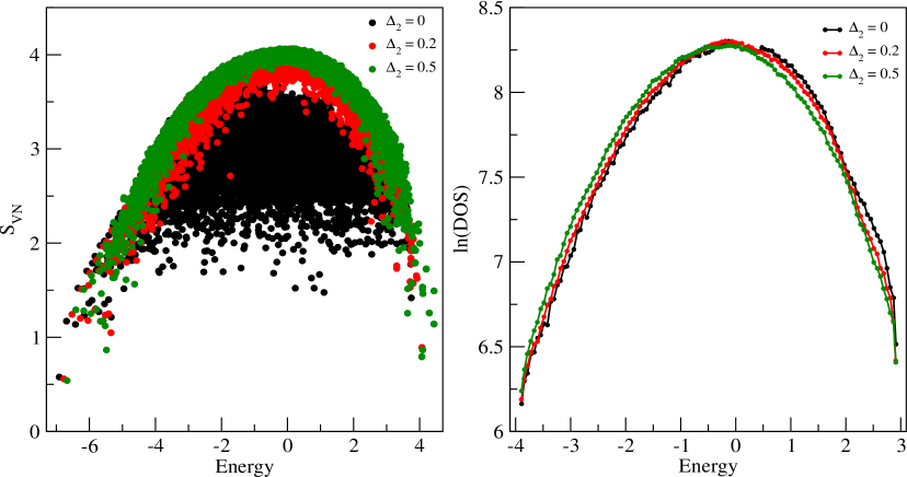
Figure 2: The subsystem VN entropy ($S_{VN}$) for individual eigenkets and $\ln(DOS)$ are plotted against the energy of the full system. Here total system size is 16 and subsystem size is 6.

IV.1 Isolated quantum system

As discussed in Sec. II.3, an isolated quantum system will be in a mixed state, for one or multiple reasons. Using the principle of equal a priori probabilities, one can show that the VN entropy is equal to the qBN entropy (which in turn is equivalent to the TH entropy).

Assume that we prepare a system in such a way that its energy lies in the narrow energy shell $(E,E+\Delta E]$, where $\Delta E$ is arbitrary but macroscopically small and microscopically large [5]. Let $\{\ket{n}\}$ be the set of the eigenkets of the system Hamiltonian, and $E_{n}$ be the eigenvalue corresponding to $\ket{n}$. The system will be in any state $\ket{n}$ with equal probability if $E_{n}\in(E,E+\Delta E]$. Accordingly, the thermodynamic entropy ($S_{TH}$), or equivalently, the quantum Boltmann entropy ($S_{qBN}$) is,

$$S_{TH}\equiv S_{qBN}=k_{B}\ln D,$$ (8)

where $D$ is the number of eigenvalues within the shell. It may be noted here that one can subdivide the energy shell into different macrostates (subspaces), with one of them having the largest number of microststes (the largest dimension) [7, 5]. For a thermodynamically large system, the dimension of this largest subspace, which corresponds to the thermal equilibrium, is essentially equal to the dimension of the shell ($D$).

Now to calculate the corresponding von Neumann entropy ($S_{VN}$) of the isolated quantum system, we note that the system is in a mixed state, represented by the following density matrix,

$$\rho=\sum_{\begin{subarray}{c}n\\ E_{n}\in\left(E,E+\Delta E\right]\end{subarray}}p_{n}\ket{n}\bra{n},$$ (9)

where $p_{n}$ is the probability to find the system in state $\ket{n}$. Since $\Delta E$ is macroscopically small, all the accessible microstates (here, eigenkets) will essentially have almost the same energy. Application of the principle of equal a priori probabilities suggests that $p_{n}=\frac{1}{D}$. As $S_{VN}=-k_{B}\text{Tr}(\rho\ln\rho)$, we need the eigenvalues of $\rho$ to efficiently compute $S_{VN}$. It is clear from Eq. 9 that $\ket{n}$ is an eigenket of $\rho$ with eigenvalue $\frac{1}{D}$, i.e., $\rho\ket{n}=\frac{1}{D}\ket{n}$ for any energy eigenket from the shell. This implies that

$$S_{VN}=-k_{B}\text{Tr}(\rho\ln\rho)=k_{B}\ln D.$$ (10)

We see from Eqs. 8 and 10 that, for an isolated quantum system, the VN entropy is the same as the TH entropy ($S_{VN}=S_{qBN}\equiv S_{TH}$), provided that the system is large and in thermal equilibrium. The detail discussion on the conditions under which this equivalence works can be found in Sec. II.2.

IV.2 Weakly interacting open quantum system

Here we consider an open system which is in contact with the thermal bath. Although the system exchanges heat with the bath, we assume that the interaction with the bath is so weak that the energy spectrum of the system is more or less unaffected by the interaction, and the dynamics of the quantum system can still be described (at-least effectively) by its Hamiltonian.

As before, let $\{E_{n}\}$ be the set of eigenvalues of the system Hamiltonian with $\ket{n}$ being the eigenket corresponding to eigenvalue $E_{n}$. In the spirit of Gibbs distribution for classical system, we can define the probability to find the system with energy $E_{n}$ as $p_{n}=\frac{1}{Q}e^{-\beta E_{n}}$, where $Q$ is the partition function, $Q=\sum_{n}e^{-\beta E_{n}}$. Here $\beta$ denotes the inverse temperature. We can now get the TH entropy, quantified by the quantum Gibbs entropy, as,

$$S_{TH}\equiv S_{qGB}=-k_{B}\sum_{n}p_{n}\ln{p_{n}}.$$ (11)

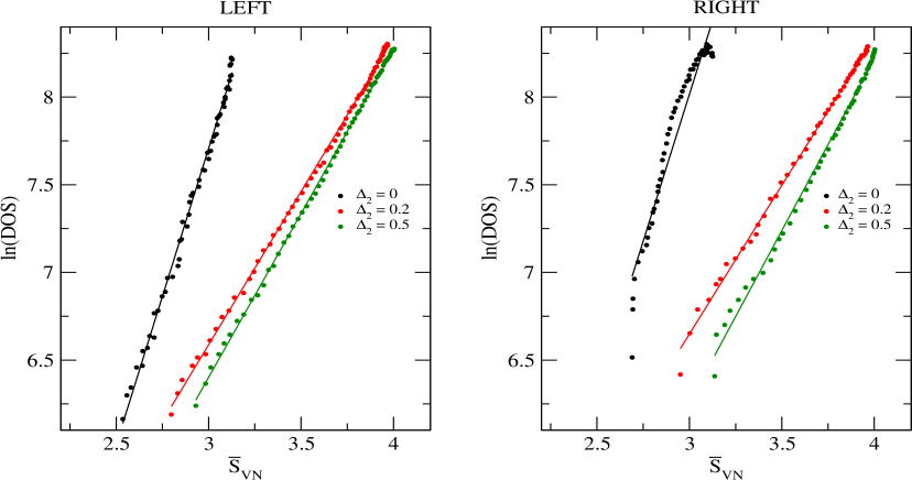
Figure 3: The average VN entropy ($\overline{S}_{VN}$) for subsystem is plotted against $\ln(DOS)$ across the energy spectrum (separately for the left and the right halves of the spectrum). Our system size is 16 and subsystem size is 6.

To find the VN entropy of the open system, one takes the following density operator: $\rho=\frac{e^{-\beta H}}{Tr(e^{-\beta H})}$, where the inverse temperature can be fixed by solving the equation $Tr(He^{-\beta H})=U$ with $U$ being the (given) internal or average energy. In fact, for overwhelmingly large number of the pure states (of the system-bath combination), it can be quite generally shown that, a weakly interacting open quantum system is very well described by a (reduced) density matrix which is equivalent to the known Gibbsian distribution [29, 30]. As a result, the VN entropy of the open system is,

$$S_{VN}=-k_{B}\text{Tr}(\rho\ln\rho)=-k_{B}\sum_{n}p_{n}\ln{p_{n}},$$ (12)

where the expression of $p_{n}$ is the same as the one appears in the formula for $S_{qGB}$ in Eq. 11. We now see from Eqs. 11 and 12 that the the VN entropy is the same as the TH entropy ($S_{VN}=S_{qBN}\equiv S_{TH}$) for a weakly interacting open quantum system in thermal equilibrium. The detail discussion on the conditions under which this equivalence works can be found in Sec. II.2.

IV.3 Subsystem of a quantum system

As mentioned in the beginning of this section (Sec. IV), it is non-trivial to verify if the VN entropy is equivalent to the TH entropy for a subsystem (of a much larger quantum system in thermal equilibrium). We analyze this possibility here.

We consider a large composite quantum system $AB$ in a state described by the density matrix $\rho$. We also assume that the subsystem $A$ is macroscopically large but much smaller compare to its counterpart $B$. We here show, mainly by the numerical analysis, that the VN entropy of the subsystem $A$ is proportional to its TH entropy.

To first calculate the TH entropy of a subsystem, we again assume that the total system is prepared with an energy lying in $(E,E+\Delta E]$. As discussed earlier, the system will be in a mixed state $\rho$, as appear in Eq. 9. The TH entropy (qBN entropy) of the full system is $S_{TH}\equiv S_{qBN}=k_{B}\ln D$, as in Eq. 8, where the $D$ is the number of eigenvalues of the system lying in the aforementioned energy shell. Now since the TH entropy is additive, we can assume that the TH entropy of the subsystem (denoted as $S^{sb}_{TH}$ ) is proportion to $k_{B}\ln D$ or to the $k_{B}\ln(DOS)$, where $DOS$ is the density-of-states of the full system at the energy scale $E$. Accordingly,

$$S^{sb}_{TH}\propto k_{B}\ln(DOS),$$ (13)

where the proportionality constant depends on the size of the subsystem in comparison to the size of the full system.

Now to calculate the VN entropy of the subsystem, we first need to calculate the reduced density matrix of the subsystem $\rho_{A}=\text{Tr}_{B}(\rho)$, where $\rho$ is the density matrix of the full system, as given in Eq. 9 (with $p_{n}=\frac{1}{D}$). Denoting the reduced density matrix corresponding to the eigenket $\ket{n}$ by $\rho_{A}^{(n)}$, where $\rho_{A}^{(n)}=\text{Tr}_{B}(\ket{n}\bra{n})$, we have

$$\rho_{A}=\frac{1}{D}\sum_{n}\rho_{A}^{(n)}.$$ (14)

Since the subsystem is in the mixed state $\rho_{A}$, we now can calculate the VN entropy of the subsystem directly from $\rho_{A}$, i.e,

$$S^{sb}_{VN}=-k_{B}\text{Tr}(\rho_{A}\ln\rho_{A}),$$ (15)

where $\rho_{A}$ is given by Eq. 14. For a system which thermalizes (or obeys the eigenstate thermalization hypothesis [21, 22]), we can also have

$$S^{sb}_{VN}=-k_{B}\text{Tr}(\rho_{A}\ln\rho_{A})\approx-\frac{k_{B}}{D}\sum_{n}\text{Tr}(\rho_{A}^{(n)}\ln\rho_{A}^{(n)}).$$ (16)

This approximate equality works since, as per the hypothesis, the expectation value of a local operator (say, $O$) is almost the same for different eigenkets from a narrow energy window, i.e., $\text{Tr}(\rho_{A}^{(n)}O)\approx\text{Tr}(\rho_{A}^{(m)}O)$. This is possible if the set of eigenvalues of the reduced density matrix $\rho_{A}^{(n)}$ is almost the same for different $n$. This implies that $\text{Tr}(\rho_{A}^{(n)}\ln\rho_{A}^{(n)})\approx\text{Tr}(\rho_{A}^{(m)}\ln\rho_{A}^{(m)})$, which guarantees the approximate equality in Eq. 16. If we write $\overline{S}_{VN}=-\frac{k_{B}}{D}\sum_{n}\text{Tr}(\rho_{A}^{(n)}\ln\rho_{A}^{(n)})$, then $S^{sb}_{VN}\approx\overline{S}_{VN}$ for a thermalized system.

We note that, if the system does not thermalize (or is integrable), then the VN entropy for the individual eigenkets ($-k_{B}\text{Tr}(\rho_{A}^{(n)}\ln\rho_{A}^{(n)})$) can take widely different values. This in fact can be seen in Fig. 2, where the subsystem VN entropy for different eigenkets are plotted against the energy across the spectrum. We here mention that, for all our numerical results, we take the following one-dimensional (with open boundary condition) Heisenberg spin-1/2 chain with the next-nearest neighbor interactions:

$$H=J\left(\sum_{i=1}^{N-1}\vec{S}_{i}\cdot\vec{S}_{i+1}+\Delta_{2}\sum_{i=1}^{N-2}S^{z}_{i}S^{z}_{i+2}\right).$$ (17)

In our calculations, we take $J=1$ and the size of the system $N=16$. This model system is integrable when $\Delta_{2}=0$ and is non-integrable (hence thermalizes) when $\Delta_{2}>0$ [31].

To make more sense of the results in Fig. 2, we plot the subsystem’s average VN entropy ($\overline{S}_{VN}$) against $\ln(DOS)$ (separately for the left and right halves of the spectrum). The results are shown in Fig. 3. We find that, for a thermalized system ($\Delta_{2}>0$), its subsystem’s average VN entropy ($\overline{S}_{VN}$) is proportional to $\ln(DOS)$ with a proportionality constant approximately equal to $\frac{N_{sb}}{N}$ (in our calculations, the subsystem size $N_{sb}=6$ and the full system size $N=16$). This proportionality constant takes a different value (a smaller one) if the system is not thermalized. We take $k_{B}=1$ for all our numerical calculations of entropy. Thus our numerical results suggest that,

$$S^{sb}_{VN}\approx\overline{S}_{VN}\propto\ln(DOS).$$ (18)

From Eqs. 13 and 18, we conclude that, like for isolated and open systems, for a subsystem also the VN entropy is equivalent to the TH entropy (qBN entropy), i.e., $S^{sb}_{VN}\equiv S^{sb}_{TH}$.

It may be worth mentioning here that, the result that the subsystem’s average VN entropy is proportional to system’s $\ln(DOS)$, is earlier reported in [32] in a different context. We also note that, elsewhere [33], the thermodynamic entropy of a subsystem is defined as what we call here $S^{sb}_{VN}$. As discussed in this work, thermodynamic (TH) entropy is appropriately calculated as the logarithm of $DOS$ (since, $S_{TH}\equiv S_{qBN}$ under some general conditions).

V Conclusion

In this work we analyze whether and when the von Neumann (VN) entropy is equal or equivalent to the thermodynamic (TH) entropy. In reviewing the major objections about the VN entropy, we explain that the concerns about the time-invariance and subadditivity properties can be addressed convincingly. We show in this study that, for large thermalized isolated or open system, the VN entropy is equivalent to the TH entropy. Next, through numerical analysis, we also show that the VN entropy of a subsystem of a large thermalized system is equivalent to its TH entropy (qBN entropy).

References

- Gogolin and Eisert [2016] C. Gogolin and J. Eisert, Equilibration, thermalisation, and the emergence of statistical mechanics in closed quantum systems, Rept. Prog. Phys. 79, 056001 (2016).
- D’Alessio et al. [2016] L. D’Alessio, Y. Kafri, A. Polkovnikov, and M. Rigol, From quantum chaos and eigenstate thermalization to statistical mechanics and thermodynamics, Adv. Phys. 65, 239 (2016).
- Reimann [2008] P. Reimann, Foundation of statistical mechanics under experimentally realistic conditions, Phys. Rev. Lett. 101, 190403 (2008).
- Kardar [2007] M. Kardar, Statistical Physics of Particles, 1st ed. (Cambridge University Press, 2007).
- Mori et al. [2018] T. Mori, T. N. Ikeda, E. Kaminishi, and M. Ueda, Thermalization and prethermalization in isolated quantum systems: a theoretical overview, J. Phys. B: At. Mol. Opt. Phys. 51, 112001 (2018).
- Pathria and Beale [2011] R. K. Pathria and P. D. Beale, Statistical Mechanics, 3rd ed. (Elsevier, 2011).
- Goldstein et al. [2019] S. Goldstein, J. L. Lebowitz, R. Tumulka, and N. Zanghì, Gibbs and boltzmann entropy in classical and quantum mechanics, in Statistical Mechanics and Scientific Explanation (World Scientific, 2019) Chap. 14.
- von Neumann [2018] J. von Neumann, Mathematical Foundations of Quantum Mechanics, New Esition (Princeton University Press, 2018).
- Landau et al. [1990] L. D. Landau, E. M. Lifshitz, and M. Pitaevskii, Statistical Physics: Part 1, 3rd ed. (Pergamon Press, Oxford, 1990).
- Shenker [1999] O. R. Shenker, Is -kTr( ln ) the entropy in quantum mechanics?, Br. J. Phil. Sci. 50, 33 (1999).
- Hemmo and Shenker [2006] M. Hemmo and O. Shenker, Von Neumann’s entropy does not correspond to thermodynamic entropy, Phil. Sci. 73, 153 (2006).
- Henderson [2003] L. Henderson, The von Neumann entropy: a reply to Shenker, Br. J. Phil. Sci. 54, 291 (2003).
- Deville and Deville [2013] A. Deville and Y. Deville, Clarifying the link between von Neumann and thermodynamic entropies, Eur. Phys. J. H 38, 57 (2013).
- Strasberg and Winter [2021] P. Strasberg and A. Winter, First and second law of quantum thermodynamics: A consistent derivation based on a microscopic definition of entropy, PRX Quantum 2, 030202 2, 030202 (2021).
- Jaynes [1957] E. T. Jaynes, Information theory and statistical mechanics. II, Phys. Rev. 108, 171 (1957).
- Facchi et al. [2021] P. Facchi, G. Gramegna, and A. Konderak, Entropy of quantum states, Entropy 23, 645 (2021).
- Sheridan [2020] E. Sheridan, A man misunderstood: Von Neumann did not claim that his entropy corresponds to the phenomenological thermodynamic entropy, ArXiv 10.48550/arXiv.2007.06673 (2020).
- Šfránek et al. [2021] D. Šfránek, A. Aguirre, J. Schindler, and J. M. Deutsch, A brief introduction to observational entropy, Found. Phys. 51, 101 (2021).
- Sakurai and Napolitano [2021] J. J. Sakurai and J. Napolitano, Modern Quantum Mechanics, 3rd ed. (Cambridge University Press, New York, 2021).
- Araki and Lieb [1970] H. Araki and E. H. Lieb, Entropy inequalities, Commun. Math. Phys. 18, 160 (1970).
- Deutsch [1991] J. M. Deutsch, Quantum statistical mechanics in a closed system, Phys. Rev. A. 43, 2046 (1991).
- Srednicki [1994] M. Srednicki, Chaos and quantum thermalization, Phys. Rev. E 50, 888 (1994).
- Pilatowsky-Cameo and Choi [2024] S. Pilatowsky-Cameo and S. Choi, Quantum thermalization of translation-invariant systems at high temperature, ArXiv 10.48550/arXiv.2409.07516 (2024).
- Mölter et al. [2014] J. Mölter, T. Barthel, U. Schollwöck, and V. Alba, Bound states and entanglement in the excited states of quantum spin chains, J. Stat. Mech. , P10029 (2014).
- Alba et al. [2009] V. Alba, M. Fagotti, and P. Calabrese, Entanglement entropy of excited states, J. Stat. Mech. , P10020 (2009).
- Moudgalya et al. [2018] S. Moudgalya, N. Regnault, and B. A. Bernevig, Entanglement of exact excited states of affleck-kennedy-lieb-tasaki models: Exact results, many-body scars, and violation of the strong eigenstate thermalization hypothesis, Phys. Rev. B 98, 235156 (2018).
- Bianchi et al. [2022] E. Bianchi, L. Hackl, M. Kieburg, M. Rigol, and L. Vidmar, Volume-law entanglement entropy of typical pure quantum states, PRX Quantum 3, 030201 (2022).
- Peres [2002] A. Peres, Quantum Theory: Concepts and Methods (Kluwer Academic Publishers, New York, 2002) Chap. 9.
- Popescu et al. [2006] S. Popescu, A. J. Short, and A. Winter, Entanglement and the foundations of statistical mechanics, Nat. Phys. 2, 754 (2006).
- Goldstein et al. [2006] S. Goldstein, J. L. Lebowitz, R. Tumulka, and N. Zanghì, Canonical typicality, Phys. Rev. Lett. 96, 050403 (2006).
- Steinigeweg et al. [2013] R. Steinigeweg, J. Herbrych, and P. Prelovšek, Eigenstate thermalization within isolated spin-chain systems, Phys. Rev. E 87, 012118 (2013).
- Sahoo et al. [2012] S. Sahoo, V. M. L. D. P. Goli, S. Ramasesha, and D. Sen, Exact entanglement studies of strongly correlated systems: role of long-range interactions and symmetries of the system, J. Phys.: Condens. Matter 24, 115601 (2012).
- Deutsch et al. [2013] J. M. Deutsch, H. Li, and A. Sharma, Microscopic origin of thermodynamic entropy in isolated systems, Phys. Rev. E 87, 042135 (2013).