Nonlinear soft mode action for the large-$p$ SYK model

Abstract

The physics of the SYK model at low temperatures is dominated by a soft mode governed by the Schwarzian action. In Maldacena:2016hyu the linearised action was derived from the soft mode contribution to the four-point function, and physical arguments were presented for its nonlinear completion to the Schwarzian. In this paper, we give two derivations of the full nonlinear effective action in the large $p$ limit, where $p$ is the number of fermions in the interaction terms of the Hamiltonian. The first derivation uses that the collective field action of the large-$p$ SYK model is Liouville theory with a non-conformal boundary condition that we study in conformal perturbation theory. This derivation can be viewed as an explicit version of the renormalisation group argument for the nonlinear soft mode action in Kitaev:2017awl . The second derivation uses an Ansatz for how the soft mode embeds into the microscopic configuration space of the collective fields. We generalise our results for the large-$p$ SYK chain and obtain a “Schwarzian chain” effective action for it. These derivations showcase that the large-$p$ SYK model is a rare system, in which there is sufficient control over the microscopic dynamics, so that an effective description can be derived for it without the need for extra assumptions or matching (in the effective field theory sense).

1 Introduction and summary

The Sachdev-Ye-Kitaev (SYK) model KitaevTalks ; Sachdev:2015efa ; Maldacena:2016hyu and its generalisations Gu:2016oyy ; Davison:2016ngz ; Fu:2016vas ; Gross:2017vhb ; Murugan:2017eto ; Lian:2019axs ; Milekhin:2021sqd ; Milekhin:2021cou ; Berkooz:2021ehv ; Berkooz:2022dfr provide a rare analytically solvable window into many-body quantum chaos. The computation of out-of-time-ordered correlation functions in these models has led to many new insights into the quantum butterfly effect Shenker:2013pqa ; Roberts:2014isa ; Maldacena:2015waa and operator growth Roberts:2018mnp ; Qi:2018bje ; Parker:2018yvk . Its low energy description in terms of the Schwarzian effective theory uncovered the Nearly-CFT₁ universality class of quantum dynamics, and its holographic dual JT gravity description Jensen:2016pah ; Maldacena:2016upp .

In the low temperature limit, the dynamics of the SYK model is dominated by a soft mode that encodes the reparametrisations of time. In quantum mechanics the analog of the infinite dimensional conformal symmetry of two-dimensional CFTs is the reparametrisation symmetry of time: however it cannot be a true symmetry in a system with nontrivial dynamics. The breaking of this symmetry is controlled by the Schwarzian action for the reparametrisations of time with a prefactor that scales linearly with the temperature, which explains the importance of this mode at low temperatures:

$$S=-\frac{N\alpha_{S}}{\beta\mathcal{J}}\int_{0}^{2\pi}du\,\textrm{Sch}\left[\tan\left(f/2\right),u\right]\,,$$ (1)

where $N$ is the number of fermions, $\alpha_{S}$ is a dimensionless number, $\beta$ is the inverse temperature, $\mathcal{J}$ is the dimensionful coupling strength of the SYK model, $u={2\pi\over\beta}\tau$, $f(u)$ is the time reparametrisation mode, and Sch$[h,u]={h^{\prime\prime\prime}(u)\over h^{\prime}(u)}-\frac{3}{2}\left({h^{\prime\prime}(u)\over h^{\prime}(u)}\right)^{2}$ is the Schwarzian derivative.

The results described above were argued for convincingly in several different ways Maldacena:2016hyu ; Bagrets:2016cdf ; Kitaev:2017awl ; Rosenhaus:2018dtp : we give a quick review of the two most detailed arguments below. The key complication in these derivations is the matching between the UV and the IR, low temperature behaviour of the collective fields, which can only be done indirectly (and involves the constant ${\alpha}_{S}$ that can only be determined numerically). In the large $p$ limit of the SYK model the UV to IR connection is under much better control. In this paper we capitalise on this fact to give two explicit analytical derivations of the nonlinear Schwarzian action, including its prefactor.

In Maldacena:2016hyu , the leading connected contribution to the four point function of fermions was computed by summing ladder diagrams. Taking a strict IR limit of the ladder diagrams produces a divergence. The origin of this divergence is that reparametrisations of time is a spontaneously broken symmetry, and the associated Goldstone boson has zero action (due to the low dimensionality of the problem). Backing away from the IR leads to explicit breaking and makes time reparametrisations pseudo-Goldstone bosons. They contribute to the four point function through the propagator of small fluctuations around the saddle $\expectationvalue{{{\delta}}f(u){{\delta}}f(0)}$, where ${{\delta}}f(u)$ is defined through $f(u)=u+{{\delta}}f(u)$. This propagator can be read off from the ladder diagrams, and it matches with the prediction of the linearisation of (1), with numerical input required to fix ${\alpha}_{S}$ for general $p$, and ${\alpha}_{S}={1\over 4p^{2}}$ for large $p$. In Maldacena:2016hyu a further symmetry argument is presented for the nonlinear completion to the full Schwarzian action (1).

In Kitaev:2017awl , an alternative argument is presented for the nonlinear Schwarzian. The collective field formulation gives rise to a nonlocal action, which then is separated into two parts, one that is time reparatmetrisation invariant, and a deformation that breaks this symmetry. The latter term is large, but it is argued that it can be replaced by a small deformation in the IR regime (with ${\alpha}_{S}$ fixed by numerics), and the Schwarzian action is obtained this way. We regard our first argument as a close relative of the argument of Kitaev:2017awl . However the large $p$ limit we consider is more controlled: the collective field formulation leads to a local conformal action (in two times), and it is only boundary conditions that break the reparametrisation symmetry. We can then use boundary CFT (BCFT) renormalisation group technology to derive the Schwarzian action.

The outline of the paper is as follows. In Sec. 2 we provide a brief review of the SYK model, highlighting the infrared regime and the emergence of a time reparametrisation soft mode and how its action breaks reparametrisation invariance. In Sec. 3 we then describe the large $p$ limit, which is characterised by a Liouville action with non-conformal boundary conditions. In particular, in Sec. 4 we show that the saddle point of this theory behaves like the one point function of a bulk vertex operator in a BCFT, deformed by an irrelevant boundary operator that we identify to be the displacement operator $\hat{D}$. Our first derivation consists of evaluating $\hat{D}$ on the reparametrisations of the saddle, finding that the deformation is, as expected, the Schwarzian. Our second derivation presented in Sec. 5, is less elegant, but more hands-on. We expect that this method can be generalised to other systems, where the Schwarzian is expected to emerge. It consists of building an Ansatz for the microscopic field configuration, and plugging it into the Liouville action. In particular, we look for a configuration that obeys the following criteria: its starting point is the reparametrisation of the thermal saddle restricted to obey the Kubo–Martin–Schwinger (KMS) condition and deformed to satisfy the non-conformal boundary conditions. Having found a configuration that follows the outlined criteria, we can compute its action: once again we recover the Schwarzian action. Finally, we study the SYK chain in Sec. 6. We derive its soft mode action using both of our methods: from the perspective of conformal perturbation theory the inter-site coupling in the chain corresponds to the addition of a marginal operator to two decoupled Liouville BCFTs, while it is straightforward to make our Ansatz space-dependent and to evaluate the SYK chain action on it. Both methods lead to the same soft mode action that we call the Schwarzian chain:

$$\begin{split}S=-\frac{N}{4p^{2}}\sum_{x=0}^{M-1}&\Biggl{[}(\pi\delta v)\int_{0}^{2\pi}d\tau\,\textrm{Sch}[\tan(f_{x}/2),\tau]+\\ &+\alpha\int d\tau_{1}d\tau_{2}\Biggl{[}\frac{\sqrt{f_{x}^{\prime}\left(\tau_{1}\right)}\sqrt{f_{x}^{\prime}\left(\tau_{2}\right)}}{\sqrt{\sin^{2}\left(\frac{f_{x}\left(\tau_{1}\right)-f_{x}\left(\tau_{2}\right)}{2}\right)}}\frac{\sqrt{f_{x+1}^{\prime}\left(\tau_{1}\right)}\sqrt{f_{x+1}^{\prime}\left(\tau_{2}\right)}}{\sqrt{\sin^{2}\left(\frac{f_{x+1}\left(\tau_{1}\right)-f_{x+1}\left(\tau_{2}\right)}{2}\right)}}\Biggr{]}\,,\end{split}$$ (2)

where $f_{x}$ is the reparametrisation degree of freedom for site $x$, $M$ is the number of lattice sites, and ${\alpha}$ is the inter-site coupling. Note that the inter-site coupling leads to an action is non-local in time, as was discussed before in Almheiri:2019jqq ; Milekhin:2021sqd ; Milekhin:2021cou .

Note added: During the final stages of our work we learned about an independent work by Berkooz, Frumkin, Mamroud, and Seitz Berkooz:toappear that also derives the nonlinear Schwarzian using a similar Ansatz to the one we use in our second derivation. We comment briefly on the differences between the two Ansätze in Sec. 5.

2 Brief review of the SYK model

The Sachdev-Ye-Kitaev model is an ensemble of quantum mechanical models. A member of the ensemble consists of N Majorana fermions with $p$-body interactions and is described by the following Hamiltonian:

$$H=\sum_{1\leq i_{1}\leq i_{2}\leq...\leq i_{p}\leq N}J_{i_{1}i_{2}...i_{p}}\Psi_{i_{1}}...\Psi_{i_{p}},$$ (3)

where the coupling $J_{i_{1},...i_{p}}$ has a Gaussian distribution with

$$\begin{split}\langle J_{i_{1}...i_{p}}\rangle&=0\,,\\ \langle J_{i_{1}...i_{p}}^{2}\rangle=\frac{J^{2}(p-1)!}{N^{p-1}}&=\frac{2^{p-1}}{p}\frac{\mathcal{J}^{2}(p-1)!}{N^{p-1}}\,.\end{split}$$ (4)

In the large $N$ limit with annealed disorder, we can realise the average over the disorder ensemble for $J_{i_{1},...,i_{p}}$, by directly averaging the partition function Sachdev_1993 . We find the following action:

$$\begin{split}I[G,\Sigma]=-\frac{1}{2}\textrm{log det}(\partial_{\tau}-\Sigma)+\frac{1}{2}\int\int(\Sigma G-\frac{1}{p}J^{2}G^{p})\,.\end{split}$$ (5)

The field $G$ is the Euclidean bilinear:

$$G(\tau)=\frac{1}{N}\sum_{i}T\Psi_{i}(\tau)\Psi_{i}(0)$$ (6)

and $\Sigma$ is the self energy. Note that $G,\,\Sigma$ are fluctuating fields.

The classical equations of motion derived by extremising (5) are the Schwinger-Dyson equations:

$$\begin{split}G&=[\partial_{\tau}-\Sigma]^{-1}\,,\\ \Sigma&=J^{2}G^{p-1}\,.\end{split}$$ (7)

The solutions to these equations give the leading large $N$ value for the propagator $\expectationvalue{G(\tau)}$ and self-energy. It is easy to see that for zero coupling we get the propagator:

$$\expectationvalue{G^{\text{free}}(\tau)}=\frac{1}{2}\textrm{sgn}(\tau)\,,$$ (8)

whose small $\tau$ behaviour follows from the anticommutation relation of Majorana fermions, and hence $G(\tau)\to\frac{1}{2}\textrm{sgn}(\tau)$ as $\tau\to 0$ will be imposed as a constraint in what follows.

2.1 Low energy limit and the Schwarzian

We are interested in studying the IR regime of the SYK model. We notice that, since $\Sigma$ is proportional to $J^{2}$, in the low energy limit the term $\partial_{\tau}$ in equation (7) is negligible and can be dropped. We can then write a new set of IR equations of motion:

$$\begin{split}\int d\tau_{2}G(\tau,\tau_{2})\Sigma(\tau_{2},\tau_{1})&=-\delta(\tau-\tau_{1})\,,\\ \Sigma(\tau,\tau_{1})&=J^{2}G(\tau,\tau_{1})^{p-1}\,.\end{split}$$ (9)

This set of equations is invariant under $\tau\rightarrow f(\tau)$, provided that the fields transform as

$$\begin{split}G(\tau_{1},\tau_{2})&\rightarrow[f^{\prime}(\tau_{1})f^{\prime}(\tau_{2})]^{1/p}\,G(f(\tau_{1})f(\tau_{2}))\,,\\ \Sigma(\tau_{1},\tau_{2})&\rightarrow[f^{\prime}(\tau_{1})f^{\prime}(\tau_{2})]^{(p-1)/p}\,\Sigma(f(\tau_{1})f(\tau_{2}))\,.\end{split}$$ (10)

This reparametrisation invariance is then explicitly broken once we take into account the $\partial_{\tau}$ term that we discarded in the IR limit. In particular, the violation of this symmetry was argued to be described by the following action KitaevTalks ; Maldacena:2016hyu ; Kitaev:2017awl :

$$S=-\frac{N\alpha_{S}}{\mathcal{J}}\int du\,\textrm{Sch}[f,u]\,,$$ (11)

where Sch$[f,u]$ is the Schwarzian derivative and $\alpha_{s}=\frac{1}{4p^{2}}$ in the large $p$ limit. In the following, we strengthen and generalise its derivation in the large-$p$ SYK model.

3 Liouville action

To achieve better analytical control, after the large $N$ limit we take the large $p$ limit. This order of limits means that the ratio $\lambda=\frac{2p^{2}}{N}$ is infinitesimal. In order to do so, it is convenient to define the following field $g$:

$$G(\tau_{1},\tau_{2})=\frac{\textrm{sgn}(\tau_{1}-\tau_{2})}{2}\left(1+\frac{g(\tau_{1},\tau_{2})}{p}\right).$$ (12)

From this definition we see that, in order for (12) to be consistent with the small time separation limit discussed below (8), we will need to enforce the boundary condition $g(\tau_{1}=\tau_{2})=0$. Furthermore, since the bilinear should be antisymmetric for $\tau_{1}\rightarrow\tau_{2}$, $g$ needs to be symmetric: $g(\tau_{1},\tau_{2})=g(\tau_{2},\tau_{1})$. $g$ also needs to satisfy the KMS boundary conditions: $g(\tau_{1},\tau_{2}+\beta)=g(\tau_{1},\tau_{2})$ and $g(\tau_{1}+\beta,\tau_{2})=g(\tau_{1},\tau_{2})$. As shown in Cotler:2016fpe , the action for $g$ is

$$I[g]=\frac{N}{4p^{2}}\int d\tau_{1}d\tau_{2}\left[-\mathcal{J}^{2}e^{g(\tau_{1},\tau_{2})}+\frac{1}{4}\partial_{\tau_{1}}g(\tau_{1},\tau_{2})\partial_{\tau_{2}}g(\tau_{1},\tau_{2})\right],$$ (13)

which has the form of a Liouville action. Enforcing both KMS and the symmetry condition for $g$ restricts our region of integration to the shaded diamond in figure (1), with the boundary condition $g(\tau_{1}=\tau_{2})=0=g(\tau_{1}=\tau_{2}-\beta)$ and the identification $g(x,\beta-x)=g(\beta-x,\beta+x)$, and with the prefactor in equation (13) now becoming $\frac{N}{2p^{2}}$. Since this prefactor is large, it is useful to analyse the saddle point:

$$e^{g_{*}(\tau_{1},\tau_{2})}=\left(\frac{\cos\left[\frac{\pi v}{2}\right]}{\cos\left[\pi v\left(\frac{1}{2}-\frac{|\tau_{1}-\tau_{2}|}{\beta}\right)\right]}\right)^{2}\,,$$ (14)

where $v$ is defined through the equation:

$$\begin{split}\beta\mathcal{J}=\frac{\pi v}{\textrm{cos}\frac{\pi v}{2}}\,.\end{split}$$ (15)

Note that the low energy limit, $\beta\mathcal{J}\gg 1$, corresponds to the regime where $v\rightarrow 1$. It will then be convenient to redefine $v=1-\delta v$ and then take $\delta v\rightarrow 0$. We will also work with the following set of coordinates:

$$\begin{split}\delta\tau&=\tau_{2}-\tau_{1}\,,\\ \bar{\tau}&=\frac{\tau_{2}+\tau_{1}}{2}\,.\\ \end{split}$$ (16)

It is convenient for us to work with a rescaled field, $\gamma$:

$$e^{\gamma(\delta\tau,\bar{\tau})}=\left({\beta\mathcal{J}\over 2\pi}\right)^{2}e^{g(\delta\tau,\bar{\tau})}.$$ (17)

From now on we set $\beta=2\pi$, which can be reinstated using dimensional analysis. The action for $\gamma$ can be derived from (13):

$$I[\gamma]=\frac{N}{2p^{2}}\int d\tau_{1}d\tau_{2}\left[-e^{\gamma(\tau_{1},\tau_{2})}+\frac{1}{4}\partial_{\tau_{1}}\gamma(\tau_{1},\tau_{2})\partial_{\tau_{2}}\gamma(\tau_{1},\tau_{2})\right].$$ (18)

Note that in equation (18), the explicit dependence on $\mathcal{J}$ has been reabsorbed into $\gamma$: now it only appears in the boundary conditions

$$\gamma(0,\bar{\tau})=\textrm{log}[\mathcal{J}^{2}].$$ (19)

The saddle point for this field is

$$e^{\gamma_{*}(\delta\tau,\bar{\tau})}=\left(\frac{v}{2\cos\left[v\left(\frac{\pi-\delta\tau}{2}\right)\right]}\right)^{2}.$$ (20)

Figure 1: Region of integration when $\beta$ is set to $2\pi$. Taking into account both KMS and the symmetry condition for $g$, we need to integrate only over the shaded region to get the correct action. Moreover, these conditions imply the identification of the two blue points $g(x,2\pi-x)=g(2\pi-x,2\pi+x)$.

3.1 Reparametrisations for the Liouville action

We note that the Liouville action is invariant under reparametrisations of the form

$$\tau_{1}\rightarrow f(\tau_{1})\,,\qquad\tau_{2}\rightarrow h(\tau_{2})\,,$$ (21)

provided that:

$$\gamma(\tau_{1},\tau_{2})\rightarrow\gamma(\tau_{1},\tau_{2})+\textrm{log}\left[f^{\prime}(\tau_{1})\right]+\textrm{log}\left[h^{\prime}(\tau_{2})\right].$$ (22)

This statement is equivalent to (10).

Let us start by looking at the reparametrised saddle:

$$e^{\tilde{\gamma}}=\frac{v^{2}}{4\cos^{2}\left[v\frac{\pi+f(\tau_{1})-h(\tau_{2})}{2}\right]}f^{\prime}(\tau_{1})h^{\prime}(\tau_{2}).$$ (23)

Imposing $\gamma(\tau_{1},2\pi-\tau_{1})=\gamma(2\pi-\tau_{1},2\pi+\tau_{1})$ results in the following set of equations:

$$\begin{split}-f(\tau_{1})+h(2\pi-\tau_{1})&=f(2\pi-\tau_{1})-h(2\pi+\tau_{1})+2\pi\,,\\ \quad f^{\prime}(\tau_{1})h^{\prime}(2\pi-\tau_{1})&=f^{\prime}(2\pi-\tau_{1})h^{\prime}(2\pi+\tau_{1}),\end{split}$$ (24)

which in turn imply

$$\begin{split}f(\tau_{1})&=h(\tau_{1})\,,\\ f(\tau_{1}+2\pi)&=f(\tau_{1})+2\pi\,,\\ f^{\prime}(\tau_{1}+2\pi)&=f^{\prime}(\tau_{1})\,.\end{split}$$ (25)

Thus we are left with one reparametrisation symmetry. This is also explicitly broken by the boundary condition $\gamma(\tau_{1}=\tau_{2})=\textrm{log}[\mathcal{J}^{2}].$ However, in the strong coupling $\mathcal{J}\to\infty$ limit the boundary condition is conformal and the symmetry is restored. This fact motivates our first approach.

4 Boundary CFT approach to the Schwarzian

We can give a short, abstract derivation of the Schwarzian action based on boundary CFT (BCFT). The Liouville theory in (12) is a CFT. Here we are considering it on a Mobius strip, equipped with non-conformal boundary conditions

$$\begin{split}e^{\gamma(\bar{\tau},{{\delta}}\tau=0)}=\mathcal{J}^{2}\,.\end{split}$$ (26)

Below we explain that for small $\delta v$ this boundary condition is close to the ZZ conformal boundary condition, and we can account for the difference using (boundary) conformal perturbation theory.

The ZZ BCFT on the half space ${{\delta}}\tau>0$ (and $\bar{\tau}$ unrestricted) is defined by the boundary condition

$$\begin{split}e^{\gamma}\sim\frac{1}{{{\delta}}\tau^{2}}\,.\end{split}$$ (27)

The behaviour of the saddle point (20) in the regime $\delta v\lesssim{{\delta}}\tau\ll\beta$ is:

$$\begin{split}e^{\gamma_{*}(\bar{\tau},{{\delta}}\tau)}&=\langle e^{\gamma}\rangle=\frac{1}{(\pi\delta v+{{\delta}}\tau)^{2}}+\dots\\ &=\frac{1}{{{\delta}}\tau^{2}}-\frac{2\pi\delta v}{{{\delta}}\tau^{3}}+\dots\,.\end{split}$$ (28)

We observe that this is the one point function of the bulk vertex operator $e^{\gamma}$ in the ZZ BCFT deformed by an irrelevant operator, since the perturbation grows towards the boundary ${{\delta}}\tau\to 0$ and is negligible for large ${{\delta}}\tau$.

Let us denote the irrelevant boundary operator as $\hat{\cal O}$. We can then write

$$\begin{split}\langle e^{\gamma}\rangle&=\langle e^{\gamma}\rangle_{\text{ZZ}}+\lambda\int d\bar{\tau}\,\langle\hat{\cal O}(\bar{\tau})e^{\gamma}\rangle_{\text{ZZ}}+\dots\\ &=\langle e^{\gamma}\rangle_{\text{ZZ}}+\lambda\int d\bar{\tau}\,\frac{\alpha}{{{\delta}}\tau^{2-\hat{{\Delta}}}\,({{\delta}}\tau^{2}+\bar{\tau}^{2})^{\hat{{\Delta}}}}+\dots\\ &=\frac{1}{{{\delta}}\tau^{2}}+\frac{\lambda\alpha^{\prime}}{{{\delta}}\tau^{1+\hat{{\Delta}}}}+\dots\,,\end{split}$$ (29)

where in the second line we used the general form of a boundary bulk two point function from McAvity:1995zd and in the third line we have absorbed some $\hat{{\Delta}}$ dependent factors into $\alpha^{\prime}$. We conclude that we are looking for a boundary operator with dimension $\hat{{\Delta}}=2$.

Either from this computation or from simply looking at the first line of (28) we identify $\hat{\cal O}=\hat{D}$, the displacement operator. The displacement operator has a nice geometric action: it locally moves the boundary inwards by a unit distance. Since the ZZ boundary was moved outwards by $\pi\delta v$, we find that $\lambda=-\pi\delta v$. We conclude that we are studying the deformed BCFT

$$\begin{split}S_{\text{ZZ}}-\pi\delta v\int d\bar{\tau}\,\hat{D}(\bar{\tau})+\dots\,.\end{split}$$ (30)

Liouville theory with ZZ boundary conditions has an infinite set of saddle points, since the reparametrisations of $\gamma_{*}$ (see section 3.1),

$$e^{\gamma^{(f)}}=\frac{f^{\prime}(\tau_{1})f^{\prime}(\tau_{2})}{\sin^{2}\left(\frac{f(\tau_{1})-f(\tau_{2})}{2}\right)}$$ (31)

also satisfy the ZZ boundary conditions. Hence they have the same action as $\gamma_{*}$. To first order in perturbation theory, we then only need to evaluate $\hat{D}(\bar{\tau})$ on this family of saddle points. To do so, we recall that $\hat{D}=T^{{{\delta}}\tau{{\delta}}\tau}|_{{{\delta}}\tau=0}$, where $T^{ab}$ is the stress tensor. Using the classic result from Dorn:2006ys that the Liouville stress tensor evaluated on a saddle $\gamma$ is

$$\begin{split}T_{11}(\tau_{1})=\frac{N}{4p^{2}}\,e^{\gamma/2}\partial_{11}e^{-\gamma/2}\,,\qquad T_{22}(\tau_{2})=\frac{N}{4p^{2}}\,e^{\gamma/2}\partial_{22}e^{-\gamma/2}\,,\end{split}$$ (32)

and plugging in the saddle (31), we obtain that

$$\begin{split}T_{11}(\tau)=T_{22}(\tau)=\frac{N}{8p^{2}}\,\textrm{Sch}[\tan(f/2),\tau]\,.\end{split}$$ (33)

Transforming these components into $T^{{{\delta}}\tau{{\delta}}\tau}=T_{11}+T_{22}$ and evaluating at ${{{\delta}}\tau=0}$, we get that

$$-\pi\delta v\int d\bar{\tau}\,\hat{D}(\bar{\tau})\big{|}_{\gamma^{(f)}}=-\frac{N\pi\delta v}{4p^{2}}\int d\bar{\tau}\,\textrm{Sch}[\tan(f/2),\bar{\tau}]\,,$$ (34)

which is, as expected just the thermal Schwarzian, $\textrm{Sch}[\tan(f/2),\tau]$. We now need to compare $\frac{N\delta v\pi}{4p^{2}}$ to $\frac{N\alpha_{s}}{\mathcal{J}}=\frac{N}{4p^{2}\mathcal{J}}$ from equation (11). From eq (14), we can see that, in the IR limit, $\frac{1}{\mathcal{J}}=\pi\delta v+O(\delta v)^{2}$: it is then clear that the two coefficients are the same. Note that from the ${{\delta}}\tau=0$ boundary we get an integral over $\bar{\tau}\in(\pi,2\pi)$, while from the ${{\delta}}\tau=2\pi$ boundary we get an integral over $\bar{\tau}\in(0,\pi)$: together they complete the thermal circle.

We conclude that the infinite set of saddle points (31) are lifted at linear order in ${{\delta}}v$. The set of field configurations is vastly larger than this soft direction. However, the orthogonal “hard directions” have an action that is $O(N/p^{2})$, which is large in the large-$p$ SYK model. The fluctuations in these directions can then be set to their saddle point value zero. Fluctuations in the reparametrisation direction in field space are enhanced by their small action (relative to other modes), and become $O(1)$ in the ultra-low temperature regime ${{\delta}}v=O(p^{2}/N)$, where their action is $O(1)$.

5 An alternative derivation for the Schwarzian

As outlined in section 3.1, the Liouville action is invariant under independent reparametrisations of $\tau_{1}$ and $\tau_{2}$, which then get restricted to one reparametrisation by the KMS condition. The remaining diagonal reparametrisation symmetry is broken by the boundary conditions at $\tau_{1}=\tau_{2}$. The goal for this section is to find the action that describes the behaviour of the reparameterisation modes, starting from (18): this is an alternative way of deriving the Schwarzian action. In order to perform this computation, we first want to find a field configuration that includes reparametrisations of the saddle point and that obeys both the boundary conditions and KMS.

5.1 Field configuration

We start from the reparametrised saddle (23), but with the constraint $f(\tau_{1})=h(\tau_{1})$ imposed by the KMS symmetry discussed in (25):

$$e^{\tilde{{\gamma}}}=\frac{v^{2}}{4\cos^{2}\left[v\frac{\pi+f(\tau_{1})-f(\tau_{2})}{2}\right]}f^{\prime}(\tau_{1})f^{\prime}(\tau_{2})\,.$$ (35)

This field configuration violates the boundary conditions. However, if we take the $v\to 1$ limit, we get that the violation is $f$ independent:

$$e^{\tilde{{\gamma}}}\big{|}_{v\to 1}=\frac{f^{\prime}(\tau_{1})f^{\prime}(\tau_{2})}{4\sin^{2}\left[\frac{f(\tau_{1})-f(\tau_{2})}{2}\right]}\approx{1\over{{\delta}}\tau^{2}}\,.$$ (36)

(This is the same equation as (31).) If we divide this with the $v=1$ saddle, we get a field configuration that goes to $1$ at the boundary:

$$\frac{\sin^{2}\left(\frac{\tau_{2}-\tau_{1}}{2}\right)}{\sin^{2}\left[\frac{f(\tau_{1})-f(\tau_{2})}{2}\right]}\,f^{\prime}(\tau_{1})f^{\prime}(\tau_{2})\,.$$ (37)

We then multiply this with the $v\neq 1$ saddle to enforce the boundary conditions and produce our Ansatz (see figure 2):

$$e^{\gamma_{f}(\tau_{1},\tau_{2})}\equiv\frac{v^{2}}{4\cos^{2}\left[v\left(\frac{\pi+\tau_{1}-\tau_{2}}{2}\right)\right]}\frac{\sin^{2}\left(\frac{\tau_{2}-\tau_{1}}{2}\right)}{\sin^{2}\left(\frac{f\left(\tau_{2}\right)-f\left(\tau_{1}\right)}{2}\right)}f^{\prime}\left(\tau_{1}\right)f^{\prime}\left(\tau_{2}\right)\,.$$ (38)

This Ansatz is designed to embed the soft reparametrisation mode into the microscopic field configuration ${{\gamma}}(\tau_{1},\tau_{2})$, and hence capture the soft mode. This mode is special, a generic configuration instead has a large $O(N/p^{2})$ action, and fluctuations in the hard directions can be set to zero.

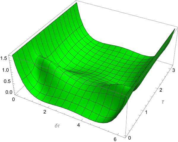
(a) Field Configuration for $v=0.8$

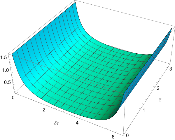
(b) Saddle Point solution for $v=0.8$

Figure 2: Three dimensional plots of $e^{{{\gamma}}_{f}(\tau_{1},\tau_{2})}$ and $e^{{{\gamma}}_{*}(\tau_{1},\tau_{2})}$ for $v=0.8$. On the left we have our Ansatz for the field configuration when $f(\tau)=\tau+0.1\sin(2\tau)+0.2\cos(3\tau)$ and on the right we are plotting the saddle point solution. By construction, both $e^{{{\gamma}}_{f}(\tau_{1},\tau_{2})}$ and $e^{{{\gamma}}_{*}(\tau_{1},\tau_{2})}$ are equal to $\mathcal{J}^{2}$ on the boundary.

Admittedly, our construction of the Ansatz is ad hoc. However, it satisfies all conditions on the field configuration, and it is a “small deformation” of the $v=1$ family of saddle points. Also, for linearised reparametrisations $f(u)=u+\varepsilon e^{-in\tau}$ it gives:

$$\begin{split}e^{-\gamma_{*}(\delta\tau,\bar{\tau})}e^{\gamma_{f}(\delta\tau,\bar{\tau})}&=1+2i\varepsilon\,f_{n}({{\delta}}\tau)e^{-in\bar{\tau}}+O(\lambda^{2})\,,\\ f_{n}({{\delta}}\tau)&={\sin{n{{\delta}}\tau\over 2}\over\tan{{{\delta}}\tau\over 2}}-n\cos{n{{\delta}}\tau\over 2}\,.\end{split}$$ (39)

The $f_{n}({{\delta}}\tau)$ functions are identical to those defined in eq. (3.109) of Maldacena:2016hyu . They realise infinitesimal reparametrisations of the $v=1$ saddle. We conclude that our Ansatz is accurate to linear order. At nonlinear order, the goal is to capture the soft direction in field space. The potential issue with the Ansatz could be that at nonlinear order in ${{\delta}}f$ it mixes with the “hard” directions. The output of our calculation will be an action that is small, $O({{\delta}}v)$, which a posteriori confirms that there is no large mixing with the hard directions. However, an $O({{\delta}}v)$ action is also consistent with an $O(\sqrt{{{\delta}}v})$ mixing with hard directions. We can verify that this does not happen in the region ${{\delta}}\tau\gg{{\delta}}v$, where our Ansatz behaves as

$$\begin{split}e^{\gamma_{f}(\delta\tau,\bar{\tau})}=&e^{\gamma_{*}}\left[1+{{{\delta}}\tau^{2}\over 6}\textrm{Sch}\left[\tan\left(f/2\right),u\right]+O\left(\delta\tau^{3}\right)\right]\,,\end{split}$$ (40)

which is the expected IR behaviour of the soft mode. We conclude that in the worst case the Ansatz deviates from the true soft mode in the region ${{\delta}}\tau\sim{{\delta}}v$, which can only result in $O({{\delta}}v)$ mixing, which is negligible. Indeed, we obtain the Schwarzian action from this Ansatz, which we know, from our first method and earlier literature, is the correct result.

The mixing issue could be further investigated by linearising around the Ansatz with a finite $f$ and finding that the zero mode of the linearised equation is indeed in the direction of the Ansatz with $f+{{\delta}}f$; we leave this computation for the future.

Note added: We briefly comment on the parallel work Berkooz:toappear . The authors consider an Ansatz distinct, but close to ours in spirit. Their Ansatz for linearised $f(u)$ gives ${\cal F}_{n}({{\delta}}\tau)$, which are the generalisation of $f_{n}({{\delta}}\tau)$ for finite ${{\delta}}v$ and reduces to them as ${{\delta}}v\to 0$. This difference is immaterial for getting the correct soft mode action at $O({{\delta}}v)$, since it amounts to a negligible $O({{\delta}}v)$ mixing with hard modes. The important difference between our Ansatz and that of Berkooz:toappear , is that the latter only satisfies the boundary conditions approximately at small ${{\delta}}v$, which the authors remedy by adding a boundary term to their action.

Before we proceed it is important to emphasise the following issue. We are interested in considering the limit for $v\rightarrow 1$: let us start by rewriting the saddle point solution as:

$$e^{\gamma_{*}(\delta\tau,\bar{\tau})}=\frac{1}{4\textrm{cos}^{2}\left[(1-\delta v)\left(\frac{\pi-\delta\tau}{2}\right)\right]}\,.$$ (41)

For finite values of $\delta\tau$, taking the limit for $\delta v$ infinitesimal is straightforward:

$$e^{\gamma_{*}(\delta\tau,\bar{\tau})}\sim\frac{1}{4\textrm{cos}^{2}\left[\frac{\pi-\delta\tau}{2}\right]}\,.$$ (42)

However, when we are close to the boundary, i.e. when $\delta\tau\sim\delta v$, things become more delicate. As in (28) we find

$$e^{\gamma_{*}(\delta\tau,\bar{\tau})}\sim\frac{1}{(\delta v\pi+\delta\tau)^{2}}\,.$$ (43)

As a result, in the following computation we will consider contributions from the bulk and from the boundary separately, paying close attention to the regime in which $\delta\tau\sim\delta v$.

5.2 Near-boundary contributions

To find the action for the reparametrisations, we plug (38) into the Liouville Lagrangian: the expression we find is not particularly illuminating, so we will not report it. As discussed, we need to consider contributions from the near-boundary region separately: we thus perform two rescalings, $\delta\tau\rightarrow\delta\tau^{\prime}\delta v$ and $\delta\tau\rightarrow 2\pi-\delta\tau^{\prime}\delta v$, and we expand around $\delta v\rightarrow 0$. We find:

$$\begin{split}S_{\textrm{bdy}}(\Lambda)=&\frac{N}{2p^{2}}\int_{0}^{\pi}d\bar{\tau}\int_{0}^{\Lambda}d\delta\tau^{\prime}\frac{\delta\tau^{\prime}(\delta\tau^{\prime}+2\pi)\left(-3f^{\prime\prime}(\bar{\tau})^{2}+f^{\prime}(\bar{\tau})^{4}+2f^{(3)}(\bar{\tau})f^{\prime}(\bar{\tau})\right)}{12(\delta\tau^{\prime}+\pi)^{2}f^{\prime}(\bar{\tau})^{2}}\delta v\\ +&\frac{N}{2p^{2}}\int_{0}^{\pi}d\bar{\tau}\int_{0}^{\Lambda}d\delta\tau^{\prime}\frac{\delta\tau^{\prime}(\delta\tau^{\prime}+2\pi)\left(-3f^{\prime\prime}(\bar{\tau}+\pi)^{2}+f^{\prime}(\bar{\tau}+\pi)^{4}+2f^{(3)}(\bar{\tau}+\pi)f^{\prime}(\bar{\tau}+\pi)\right)}{12(\delta\tau^{\prime}+\pi)^{2}f^{\prime}(\bar{\tau}+\pi)^{2}}\delta v\,,\end{split}$$ (44)

where $\Lambda$ is a large cutoff in the rescaled time ${{\delta}}\tau^{\prime}$. Integrating in $\delta\tau^{\prime}$ we get:

$$\begin{split}S_{\textrm{bdy}}(\Lambda)=&\frac{N}{2p^{2}}\int_{0}^{\pi}d\bar{\tau}\frac{\Lambda^{2}\left(-3f^{\prime\prime}(\bar{\tau})^{2}+f^{\prime}(\bar{\tau})^{4}+2f^{(3)}(\bar{\tau})f^{\prime}(\bar{\tau})\right)}{12(\Lambda+\pi)f^{\prime}(\bar{\tau})^{2}}\delta v\\ +&\frac{N}{2p^{2}}\int_{0}^{\pi}d\bar{\tau}\frac{\Lambda^{2}\left(-3f^{\prime\prime}(\bar{\tau}+\pi)^{2}+f^{\prime}(\bar{\tau}+\pi)^{4}+2f^{(3)}(\bar{\tau}+\pi)f^{\prime}(\bar{\tau}+\pi)\right)}{12(\Lambda+\pi)f^{\prime}(\bar{\tau}+\pi)^{2}}\delta v\,.\end{split}$$ (45)

Looking at the second contribution, by performing a change of variable $\bar{\tau}\rightarrow\bar{\tau}-2\pi$ we can rewrite it as:

$$\frac{N}{2p^{2}}\int_{\pi}^{2\pi}d\bar{\tau}\frac{\Lambda^{2}\left(-3f^{\prime\prime}(\bar{\tau})^{2}+f^{\prime}(\bar{\tau})^{4}+2f^{(3)}(\bar{\tau})f^{\prime}(\bar{\tau})\right)}{12(\Lambda+\pi)f^{\prime}(\bar{\tau})^{2}}\delta v\,.$$ (46)

Adding the two contributions together we get

$$S_{bdy}(\Lambda)=\frac{N}{2p^{2}}\int_{0}^{2\pi}d\bar{\tau}\frac{\Lambda^{2}\left(-3f^{\prime\prime}(\bar{\tau})^{2}+f^{\prime}(\bar{\tau})^{4}+2f^{(3)}(\bar{\tau})f^{\prime}(\bar{\tau})\right)}{12(\Lambda+\pi)f^{\prime}(\bar{\tau})^{2}}\delta v\,.$$ (47)

Note that the action in equation (47) depends on the presence of a cutoff, $\Lambda$, and is divergent for $\Lambda\rightarrow\infty$; this divergence, however, will be cured once we consider contributions from the bulk.

5.3 Bulk contributions

To compute the bulk contributions we can directly expand our Lagrangian in $\delta v$ as ${\cal L}_{bulk}={\cal L}_{bulk,0}+{{\delta}}v{\cal L}_{bulk,1}+\dots$ and consider the contributions order by order. When integrating, to avoid double counting we will include a cutoff by considering only the interval $\delta\tau\in[\Lambda\delta v,2\pi-\Lambda\delta v]$. Since the cutoff depends on ${{\delta}}v$, when integrating the term ${\cal L}_{bulk,n}$, we expect to get contributions at every order ${{\delta}}v^{m}$ with $m\geq n$. First, we integrate ${\cal L}_{bulk,0}$, and after some lengthy manipulations (see appendix A) we find:

$$S_{bulk,0}(\Lambda)=\frac{N}{2p^{2}}\int_{0}^{2\pi}d\tau\left[-\frac{\Lambda\left(-3f^{\prime\prime}(\tau)^{2}+f^{\prime}(\tau)^{4}+2f^{(3)}(\tau)f^{\prime}(\tau)\right)}{12f^{\prime}(\tau)^{2}}\delta v\right]\,.$$ (48)

Adding this contribution to eq (47), we get:

$$S_{bulk,0}(\Lambda)+S_{bdy}(\Lambda)=\frac{N}{2p^{2}}\int_{0}^{2\pi}d\tau\left[-\frac{\Lambda\pi\left(-3f^{\prime\prime}(\tau)^{2}+f^{\prime}(\tau)^{4}+2f^{(3)}(\tau)f^{\prime}(\tau)\right)}{12(\Lambda+\pi)f^{\prime}(\tau)^{2}}\delta v\right].$$ (49)

Taking the limit for $\Lambda\rightarrow\infty$ yields

$$S_{bulk,0}+S_{bdy}=\frac{N}{2p^{2}}\int_{0}^{2\pi}d\tau\left[-\frac{\pi\left(-3f^{\prime\prime}(\tau)^{2}+f^{\prime}(\tau)^{4}+2f^{(3)}(\tau)f^{\prime}(\tau)\right)}{12f^{\prime}(\tau)^{2}}\delta v\right].$$ (50)

As expected, adding contributions from the bulk cures the divergence that we had from the boundary. It is reasonable to expect that the cutoff dependence cancels at higher orders in $\delta v$ as well, and we have explicitly verified this to second order in $\delta v$.

Next, when integrating ${\cal L}_{bulk,1}$ we can set the cutoff to zero, since keeping it would only result in subleading contributions. After some manipulations (see again appendix A), we can rewrite the contribution at first order as:

$${{\delta}}v\,S_{bulk,1}=\frac{N}{2p^{2}}\int_{0}^{2\pi}d\tau\left(-\frac{\pi\left(-3f^{\prime\prime}(\tau)^{2}+f^{\prime}(\tau)^{4}+2f^{(3)}(\tau)f^{\prime}(\tau)\right)}{6f^{\prime}(\tau)^{2}}\delta v\right).$$ (51)

Adding everything together we get:

$$S=-\frac{N}{2p^{2}}\frac{\delta v\pi}{2}\int_{0}^{2\pi}d\tau\left(\frac{1}{2}f^{\prime}(\tau)^{2}+\frac{f^{(3)}(\tau)}{f^{\prime}(\tau)}-\frac{3f^{\prime\prime}(\tau)^{2}}{2f^{\prime}(\tau)^{2}}\right)=-\frac{N\delta v\pi}{4p^{2}}\int_{0}^{2\pi}d\tau\,\textrm{Sch}[\tan(f/2),\tau]\,,$$ (52)

which is in complete agreement with (34).

6 The nearest neighbour coupling in the SYK chain at low temperatures

The SYK chain consists of a chain of coupled SYK sites, with nearest neighbour interactions Gu:2016oyy . The Hamiltonian has the form:

$$H=\sum_{x=1}^{M}\biggl{(} \sum_{1\leq i_{1}\leq i_{2}\leq...\leq i_{p}\leq N}J_{x,i_{1}i_{2}...i_{p}}\Psi_{i_{1},x}...\Psi_{i_{p},x}+$$

$$\sum_{\begin{subarray}{c}1\leq i_{1}\leq i_{2}\leq...\leq i_{p/2}\leq N\\ 1\leq j_{1}\leq j_{2}\leq...\leq j_{p/2}\leq N\end{subarray}}J^{\prime}_{x,i_{1}...i_{p/2}j_{1}...j_{p/2}}\Psi_{i_{1},x}...\Psi_{i_{p/2},x}\Psi_{j_{1},x+1}...\Psi_{j_{p/2},x+1}\biggr{)}\,,$$ (53)

with:

$$\langle J^{2}_{x,i_{1},..i_{p}}\rangle=\frac{(p-1)!}{N^{p-1}}J_{0}^{2},\quad\langle J^{\prime 2}_{x,i_{1}...i_{p/2}j_{1}...j_{p/2}}\rangle=\frac{\left[(p/2)!\right]^{2}}{pN^{p-1}}J_{1}^{2},\quad\mathcal{J}^{2}_{0,1}\equiv\frac{p}{2^{p-1}}J^{2}_{0,1}\,.$$ (54)

We will identify $\mathcal{J}=\mathcal{J}_{0}$ from previous sections and define $\alpha\equiv\frac{\mathcal{J}_{1}^{2}}{\mathcal{J}^{2}}$. In the large $p$ limit we can write the action as Gu:2016oyy ; Choi:2020tdj :

$$I[g]=\frac{N}{4p^{2}}\sum_{x=0}^{M-1}\int d\tau_{1}d\tau_{2}\left[-\mathcal{J}^{2}e^{g_{x}(\tau_{1},\tau_{2})}-\mathcal{J}_{1}^{2}e^{\frac{1}{2}(g_{x}(\tau_{1},\tau_{2})+g_{x+1}(\tau_{1},\tau_{2}))}+\frac{1}{4}\partial_{\tau_{1}}g_{x}(\tau_{1},\tau_{2})\partial_{\tau_{2}}g_{x}(\tau_{1},\tau_{2})\right]\,.$$ (55)

From the perspective of conformal perturbation theory, we have started from $M$ decoupled Liouville theories on the Mobius strip and added a bulk (marginal) perturbation $e^{\frac{1}{2}(g_{x}+g_{x+1})}$. To leading order in this bulk coupling and zeroth order in ${{\delta}}v$ we can incorporate its effect by evaluating it in the reparametrised saddle configuration (31). Alternatively, our Ansatz for the field configuration in the IR regime (38) gives the same result. We get:

$$I[g]=\sum_{x=0}^{M-1} \left[-\frac{N\delta v\pi}{4p^{2}}\int_{0}^{2\pi}d\tau\,\textrm{Sch}[\tan(f_{x}/2),\tau]-\mathcal{J}_{1}^{2}\frac{N}{4p^{2}}\int d\tau_{1}d\tau_{2}\left[e^{\frac{1}{2}(g_{x}(\tau_{1},\tau_{2})+g_{x+1}(\tau_{1},\tau_{2}))}\right]\right]$$

$$=\sum_{x=0}^{M-1} \Biggl{[}-\frac{N\delta v\pi}{4p^{2}}\int_{0}^{2\pi}d\tau\,\textrm{Sch}[\tan(f_{x}/2),\tau]+$$

$$-\mathcal{J}_{1}^{2}(\pi\delta v)^{2}\frac{N}{4p^{2}}\int d\tau_{1}d\tau_{2}\Biggl{[}\frac{\sqrt{f_{x}^{\prime}\left(\tau_{1}\right)}\sqrt{f_{x}^{\prime}\left(\tau_{2}\right)}}{\sqrt{\sin^{2}\left(\frac{f_{x}\left(\tau_{1}\right)-f_{x}\left(\tau_{2}\right)}{2}\right)}}\frac{\sqrt{f_{x+1}^{\prime}\left(\tau_{1}\right)}\sqrt{f_{x+1}^{\prime}\left(\tau_{2}\right)}}{\sqrt{\sin^{2}\left(\frac{f_{x+1}\left(\tau_{1}\right)-f_{x+1}\left(\tau_{2}\right)}{2}\right)}}\Biggr{]}\,.$$ (56)

Note that we are only justified in keeping the second nonlocal term if it is the same order as the first one, since there are other modes orthogonal to $f$ that we discarded and that would give an $O(N/p^{2})$ action, not reduced by an additional factor ${{\delta}}v\ll 1$. Thus, we demand that $\mathcal{J}_{1}^{2}(\pi\delta v)^{2}\ll 1$. Note that in the IR regime $\frac{1}{\mathcal{J}_{0}}\sim\pi\delta v$, so we can write $\mathcal{J}_{1}^{2}(\pi\delta v)^{2}\sim\frac{\mathcal{J}_{1}^{2}}{\mathcal{J}_{0}^{2}}\sim\alpha$. Our requirement simply becomes $\alpha\ll 1$, with the final form of the action:

$$\begin{split}I[f]=-\frac{N}{4p^{2}}\sum_{x=0}^{M-1}&\Biggl{[}(\pi\delta v)\int_{0}^{2\pi}d\tau\,\textrm{Sch}[\tan(f_{x}/2),\tau]+\\ &+\alpha\int d\tau_{1}d\tau_{2}\Biggl{[}\frac{\sqrt{f_{x}^{\prime}\left(\tau_{1}\right)}\sqrt{f_{x}^{\prime}\left(\tau_{2}\right)}}{\sqrt{\sin^{2}\left(\frac{f_{x}\left(\tau_{1}\right)-f_{x}\left(\tau_{2}\right)}{2}\right)}}\frac{\sqrt{f_{x+1}^{\prime}\left(\tau_{1}\right)}\sqrt{f_{x+1}^{\prime}\left(\tau_{2}\right)}}{\sqrt{\sin^{2}\left(\frac{f_{x+1}\left(\tau_{1}\right)-f_{x+1}\left(\tau_{2}\right)}{2}\right)}}\Biggr{]}\,.\end{split}$$ (57)

We refer to this action as the Schwarzian chain.

Appendix A More on bulk contributions

At zeroth order in the expansion of ${\cal L}_{bulk}$, we get the following bulk contribution:

$$S_{bulk,0}(\Lambda)=\frac{N}{2p^{2}}\int_{0}^{\pi}d\bar{\tau}\int_{\Lambda\delta v}^{2\pi-\Lambda\delta v}d\delta\tau\,\mathcal{L}_{bulk,0}(\delta\tau,\bar{\tau})\,,$$ (58)

where

$$\mathcal{L}_{bulk,0}(\delta\tau,\bar{\tau})=\ (\cos(\delta\tau)+3)\csc^{2}\left(\frac{\delta\tau}{2}\right)$$

$$+\frac{2f^{\prime\prime}\left(\bar{\tau}-\frac{\delta\tau}{2}\right)\left(f^{\prime\prime}\left(\frac{\delta\tau}{2}+\bar{\tau}\right)+f^{\prime}\left(\frac{\delta\tau}{2}+\bar{\tau}\right)^{2}\cot\left(\frac{1}{2}\left(f\left(\bar{\tau}-\frac{\delta\tau}{2}\right)-f\left(\frac{\delta\tau}{2}+\bar{\tau}\right)\right)\right)\right)}{f^{\prime}\left(\bar{\tau}-\frac{\delta\tau}{2}\right)f^{\prime}\left(\frac{\delta\tau}{2}+\bar{\tau}\right)}$$

$$+\frac{f^{\prime}\left(\bar{\tau}-\frac{\delta\tau}{2}\right)}{f^{\prime}\left(\frac{\delta\tau}{2}+\bar{\tau}\right)}\biggl{(}2\frac{f^{\prime\prime}\left(\frac{\delta\tau}{2}+\bar{\tau}\right)\sin\left(f\left(\bar{\tau}-\frac{\delta\tau}{2}\right)-f\left(\frac{\delta\tau}{2}+\bar{\tau}\right)\right)}{\left(\cos\left(f\left(\bar{\tau}-\frac{\delta\tau}{2}\right)-f\left(\frac{\delta\tau}{2}+\bar{\tau}\right)\right)-1\right)}$$

$$+\frac{f^{\prime}\left(\frac{\delta\tau}{2}+\bar{\tau}\right)^{2}\left(\cos\left(f\left(\bar{\tau}-\frac{\delta\tau}{2}\right)-f\left(\frac{\delta\tau}{2}+\bar{\tau}\right)\right)+3\right)}{\left(\cos\left(f\left(\bar{\tau}-\frac{\delta\tau}{2}\right)-f\left(\frac{\delta\tau}{2}+\bar{\tau}\right)\right)-1\right)}\biggr{)}\,.$$ (59)

We can rewrite this in $\tau_{1},\tau_{2}$ coordinates:

$$\mathcal{L}_{bulk,0}(\tau_{1},\tau_{2})=\ \frac{1}{8}\biggl{(}\frac{2f^{\prime\prime}(\tau_{1})\left(f^{\prime\prime}(\tau_{2})+f^{\prime}(\tau_{2})^{2}\cot\left(\frac{1}{2}(f(\tau_{1})-f(\tau_{2}))\right)\right)}{f^{\prime}(\tau_{1})f^{\prime}(\tau_{2})}+$$

$$+\frac{2f^{\prime}(\tau_{1})\left(f^{\prime\prime}(\tau_{2})\sin(f(\tau_{1})-f(\tau_{2}))+f^{\prime}(\tau_{2})^{2}(\cos(f(\tau_{1})-f(\tau_{2}))+3)\right)}{f^{\prime}(\tau_{2})(\cos(f(\tau_{1})-f(\tau_{2}))-1)}+$$

$$+4\csc^{2}\left(\frac{\tau_{1}-\tau_{2}}{2}\right)-2\biggr{)}\,,$$ (60)

which can be rewritten as:

$$\mathcal{L}_{bulk,0}(\tau_{1},\tau_{2})=\ \partial_{\tau_{2}}\left[\frac{f^{\prime\prime}\left(\tau_{1}\right)\left(\log\left(f^{\prime}\left(\tau_{2}\right){}^{2}\right)-2\log\left(\sin^{2}\left(\frac{1}{2}\left(f\left(\tau_{1}\right)-f\left(\tau_{2}\right)\right)\right)\right)\right)}{8f^{\prime}\left(\tau_{1}\right)}\right]+$$

$$+\partial_{\tau_{1}}\biggl{[}\frac{1}{4}f^{\prime}\left(\tau_{2}\right)\left(f\left(\tau_{1}\right)+4\sin\left(\frac{f\left(\tau_{1}\right)}{2}\right)\csc\left(\frac{1}{2}\left(f\left(\tau_{1}\right)-f\left(\tau_{2}\right)\right)\right)\csc\left(\frac{f\left(\tau_{2}\right)}{2}\right)\right)+$$

$$-\frac{f^{\prime\prime}\left(\tau_{2}\right)\log\left(\sin^{2}\left(\frac{1}{2}\left(f\left(\tau_{1}\right)-f\left(\tau_{2}\right)\right)\right)\right)}{4f^{\prime}\left(\tau_{2}\right)}\biggr{]}+\frac{1}{1-\cos\left(\tau_{1}-\tau_{2}\right)}-\frac{1}{4}\,.$$ (61)

We can now evaluate the total derivatives at the boundaries of the integration intervals and expand in $\delta v$: after some computations we get (48).

The first order contribution is:

$$S_{bulk,1}=\frac{N}{2p^{2}}\int_{0}^{\pi}d\bar{\tau}\int_{0}^{2\pi}d\delta\tau\,\mathcal{L}_{bulk,1}(\delta\tau,\bar{\tau})\,,$$ (62)

with

$$\mathcal{L}_{bulk,1}(\delta\tau,\bar{\tau})=\ \frac{1}{8}\Biggl{(}f^{\prime}\left(\bar{\tau}-\frac{\delta\tau}{2}\right)$$

$$\biggl{(}2\left((\pi-\delta\tau)\cot\left(\frac{\delta\tau}{2}\right)+2\right)f^{\prime}\left(\frac{\delta\tau}{2}+\bar{\tau}\right)\csc^{2}\left(\frac{1}{2}\left(f\left(\bar{\tau}-\frac{\delta\tau}{2}\right)-f\left(\frac{\delta\tau}{2}+\bar{\tau}\right)\right)\right)+$$

$$-(-\delta\tau+\sin(\delta\tau)+\pi)\csc^{2}\left(\frac{\delta\tau}{2}\right)\cot\left(\frac{1}{2}\left(f\left(\bar{\tau}-\frac{\delta\tau}{2}\right)-f\left(\frac{\delta\tau}{2}+\bar{\tau}\right)\right)\right)\biggr{)}$$

$$+\frac{(-\delta\tau+\sin(\delta\tau)+\pi)\csc^{2}\left(\frac{\delta\tau}{2}\right)f^{\prime\prime}\left(\bar{\tau}-\frac{\delta\tau}{2}\right)}{f^{\prime}\left(\bar{\tau}-\frac{\delta\tau}{2}\right)}+2\frac{2\cos(\delta\tau)+4(\pi-\delta\tau)\cot\left(\frac{\delta\tau}{2}\right)}{\cos(\delta\tau)-1}+$$

$$+2\frac{(-\delta\tau+\sin(\delta\tau)+\pi)\left(f^{\prime\prime}\left(\frac{\delta\tau}{2}+\bar{\tau}\right)+f^{\prime}\left(\frac{\delta\tau}{2}+\bar{\tau}\right)^{2}\cot\left(\frac{1}{2}\left(f\left(\bar{\tau}-\frac{\delta\tau}{2}\right)-f\left(\frac{\delta\tau}{2}+\bar{\tau}\right)\right)\right)\right)}{f^{\prime}\left(\frac{\delta\tau}{2}+\bar{\tau}\right)(\cos(\delta\tau)-1)}+$$

$$+\frac{12}{\cos(\delta\tau)-1}\Biggr{)}\,.$$ (63)

As we noted in Sec. 5.3, there is no need to consider a cutoff, as it would only result in contributions that are subleading in $\delta v$. Rewriting eq (A) in $\tau_{1},\tau_{2}$ coordinates yields:

$$\mathcal{L}_{bulk,1}(\tau_{1},\tau_{2})=\ \frac{1}{8}\biggl{(}f^{\prime}\left(\tau_{1}\right)\biggl{(}2\left(\left(\tau_{1}-\tau_{2}+\pi\right)\cot\left(\frac{1}{2}\left(\tau_{2}-\tau_{1}\right)\right)+2\right)f^{\prime}\left(\tau_{2}\right)\csc^{2}\left(\frac{1}{2}\left(f\left(\tau_{1}\right)-f\left(\tau_{2}\right)\right)\right)+$$

$$+\left(-\tau_{1}+\tau_{2}+\sin\left(\tau_{1}-\tau_{2}\right)-\pi\right)\csc^{2}\left(\frac{1}{2}\left(\tau_{2}-\tau_{1}\right)\right)\cot\left(\frac{1}{2}\left(f\left(\tau_{1}\right)-f\left(\tau_{2}\right)\right)\right)\biggr{)}+$$

$$+\frac{\left(\tau_{1}-\tau_{2}-\sin\left(\tau_{1}-\tau_{2}\right)+\pi\right)\csc^{2}\left(\frac{1}{2}\left(\tau_{2}-\tau_{1}\right)\right)f^{\prime\prime}\left(\tau_{1}\right)}{f^{\prime}\left(\tau_{1}\right)}+$$

$$+2\frac{\left(\tau_{1}-\tau_{2}-\sin\left(\tau_{1}-\tau_{2}\right)+\pi\right)\left(f^{\prime\prime}\left(\tau_{2}\right)+f^{\prime}\left(\tau_{2}\right){}^{2}\cot\left(\frac{1}{2}\left(f\left(\tau_{1}\right)-f\left(\tau_{2}\right)\right)\right)\right)}{f^{\prime}\left(\tau_{2}\right)(\cos\left(\tau_{1}-\tau_{2}\right)-1)}+$$

$$+2\frac{\left(+2\cos\left(\tau_{1}-\tau_{2}\right)+4\left(\tau_{1}-\tau_{2}+\pi\right)\cot\left(\frac{1}{2}\left(\tau_{2}-\tau_{1}\right)\right)+6\right)}{\cos\left(\tau_{1}-\tau_{2}\right)-1}\biggr{)}\,,$$ (64)

which can be written as

$$\mathcal{L}_{bulk,1}(\tau_{1},\tau_{2})=\ \partial_{\tau_{2}}\left[\frac{\left(\tau_{1}-\tau_{2}+\pi\right)\cot\left(\frac{1}{2}\left(\tau_{1}-\tau_{2}\right)\right)f^{\prime\prime}\left(\tau_{1}\right)}{4f^{\prime}\left(\tau_{1}\right)}\right]+$$

$$+\partial_{\tau_{1}}\biggl{[}\frac{1}{8f^{\prime}\left(\tau_{2}\right)}\left(\left(\tau_{1}-2\tau_{2}+2\pi\right)\sin\left(\frac{\tau_{1}}{2}\right)-\tau_{1}\sin\left(\frac{1}{2}\left(\tau_{1}-2\tau_{2}\right)\right)\right)$$

$$\csc\left(\frac{1}{2}\left(\tau_{1}-\tau_{2}\right)\right)\csc\left(\frac{\tau_{2}}{2}\right)f^{\prime\prime}\left(\tau_{2}\right)\biggr{]}+$$

$$+\partial_{\tau_{1}}\biggl{[}\frac{1}{8}\left(\left(\tau_{1}-2\tau_{2}+2\pi\right)\sin\left(\frac{\tau_{1}}{2}\right)-\tau_{1}\sin\left(\frac{1}{2}\left(\tau_{1}-2\tau_{2}\right)\right)\right)$$

$$\,\csc\left(\frac{1}{2}\left(\tau_{1}-\tau_{2}\right)\right)\csc\left(\frac{\tau_{2}}{2}\right)f^{\prime}\left(\tau_{2}\right)\cot\left(\frac{1}{2}\left(f\left(\tau_{1}\right)-f\left(\tau_{2}\right)\right)\right)\biggr{]}+$$

$$+\partial_{\tau_{2}}\biggl{[}\frac{1}{8}\left(\tau_{2}\sin\left(\tau_{1}-\frac{\tau_{2}}{2}\right)+\left(\tau_{2}-2\left(\tau_{1}+\pi\right)\right)\sin\left(\frac{\tau_{2}}{2}\right)\right)$$

$$\,\csc\left(\frac{\tau_{1}}{2}\right)\csc\left(\frac{1}{2}\left(\tau_{1}-\tau_{2}\right)\right)f^{\prime}\left(\tau_{1}\right)\cot\left(\frac{1}{2}\left(f\left(\tau_{1}\right)-f\left(\tau_{2}\right)\right)\right)\biggr{]}+$$

$$+\partial_{\tau_{1}}\biggl{[}\frac{1}{4}\left(\tau_{2}-\pi\right)\cot\left(\frac{\tau_{2}}{2}\right)f^{\prime}\left(\tau_{2}\right)\cot\left(\frac{1}{2}\left(f\left(\tau_{1}\right)-f\left(\tau_{2}\right)\right)\right)\biggr{]}+$$

$$+\partial_{\tau_{2}}\biggl{[}-\frac{1}{4}\left(\left(\tau_{1}+\pi\right)\cot\left(\frac{\tau_{1}}{2}\right)-4\right)f^{\prime}\left(\tau_{1}\right)\cot\left(\frac{1}{2}\left(f\left(\tau_{1}\right)-f\left(\tau_{2}\right)\right)\right)\biggr{]}+$$

$$+\frac{\cos\left(\tau_{1}-\tau_{2}\right)-2\left(\tau_{1}-\tau_{2}+\pi\right)\cot\left(\frac{1}{2}\left(\tau_{1}-\tau_{2}\right)\right)+3}{2\left(\cos\left(\tau_{1}-\tau_{2}\right)-1\right)}\,.$$ (65)

As we did for the order zero contribution, we now need to evaluate the total derivatives at the boundaries of the integration intervals and after some further manipulation, we get (51).

References

- (1) J. Maldacena and D. Stanford, Remarks on the Sachdev-Ye-Kitaev model, Phys. Rev. D94 (2016) 106002, [1604.07818].
- (2) A. Kitaev and S. J. Suh, The soft mode in the Sachdev-Ye-Kitaev model and its gravity dual, JHEP 05 (2018) 183, [1711.08467].
- (3) A. Kitaev, A simple model of quantum holography, KITP strings seminar and Entanglement program (Feb. 12, April 7, and May 27) (2015) .
- (4) S. Sachdev, Bekenstein-Hawking Entropy and Strange Metals, Phys. Rev. X5 (2015) 041025, [1506.05111].
- (5) Y. Gu, X.-L. Qi and D. Stanford, Local criticality, diffusion and chaos in generalized Sachdev-Ye-Kitaev models, JHEP 05 (2017) 125, [1609.07832].
- (6) R. A. Davison, W. Fu, A. Georges, Y. Gu, K. Jensen and S. Sachdev, Thermoelectric transport in disordered metals without quasiparticles: The Sachdev-Ye-Kitaev models and holography, Phys. Rev. B 95 (2017) 155131, [1612.00849].
- (7) W. Fu, D. Gaiotto, J. Maldacena and S. Sachdev, Supersymmetric Sachdev-Ye-Kitaev models, Phys. Rev. D 95 (2017) 026009, [1610.08917].
- (8) D. J. Gross and V. Rosenhaus, A line of CFTs: from generalized free fields to SYK, JHEP 07 (2017) 086, [1706.07015].
- (9) J. Murugan, D. Stanford and E. Witten, More on Supersymmetric and 2d Analogs of the SYK Model, JHEP 08 (2017) 146, [1706.05362].
- (10) B. Lian, S. L. Sondhi and Z. Yang, The chiral SYK model, JHEP 09 (2019) 067, [1906.03308].
- (11) A. Milekhin, Coupled Sachdev-Ye-Kitaev models without Schwartzian dominance, 2102.06651.
- (12) A. Milekhin, Non-local reparametrization action in coupled Sachdev-Ye-Kitaev models, JHEP 12 (2021) 114, [2102.06647].
- (13) M. Berkooz, A. Sharon, N. Silberstein and E. Y. Urbach, Onset of quantum chaos in disordered CFTs, Phys. Rev. D 106 (2022) 045007, [2111.06108].
- (14) M. Berkooz, A. Sharon, N. Silberstein and E. Y. Urbach, Onset of Quantum Chaos in Random Field Theories, Phys. Rev. Lett. 129 (2022) 071601, [2207.11980].
- (15) S. H. Shenker and D. Stanford, Black holes and the butterfly effect, JHEP 03 (2014) 067, [1306.0622].
- (16) D. A. Roberts, D. Stanford and L. Susskind, Localized shocks, JHEP 03 (2015) 051, [1409.8180].
- (17) J. Maldacena, S. H. Shenker and D. Stanford, A bound on chaos, JHEP 08 (2016) 106, [1503.01409].
- (18) D. A. Roberts, D. Stanford and A. Streicher, Operator growth in the SYK model, JHEP 06 (2018) 122, [1802.02633].
- (19) X.-L. Qi and A. Streicher, Quantum Epidemiology: Operator Growth, Thermal Effects, and SYK, JHEP 08 (2019) 012, [1810.11958].
- (20) D. E. Parker, X. Cao, A. Avdoshkin, T. Scaffidi and E. Altman, A Universal Operator Growth Hypothesis, Phys. Rev. X 9 (2019) 041017, [1812.08657].
- (21) K. Jensen, Chaos in AdS2 Holography, Phys. Rev. Lett. 117 (2016) 111601, [1605.06098].
- (22) J. Maldacena, D. Stanford and Z. Yang, Conformal symmetry and its breaking in two dimensional Nearly Anti-de-Sitter space, PTEP 2016 (2016) 12C104, [1606.01857].
- (23) D. Bagrets, A. Altland and A. Kamenev, Sachdev–Ye–Kitaev model as Liouville quantum mechanics, Nucl. Phys. B 911 (2016) 191–205, [1607.00694].
- (24) V. Rosenhaus, An introduction to the SYK model, J. Phys. A 52 (2019) 323001, [1807.03334].
- (25) A. Almheiri and J. Polchinski, Models of AdS2 backreaction and holography, JHEP 11 (2015) 014, [1402.6334].
- (26) A. Almheiri, A. Milekhin and B. Swingle, Universal constraints on energy flow and SYK thermalization, JHEP 08 (2024) 034, [1912.04912].
- (27) M. Berkooz, R. Frumkin, O. Mamroud and J. Seitz, Twisted times, the Schwarzian and its deformations in DSSYK, (to appear) (2024) .
- (28) S. Sachdev and J. Ye, Gapless spin-fluid ground state in a random quantum heisenberg magnet, Physical Review Letters 70 (May, 1993) 3339–3342.
- (29) L. Erdős and D. Schröder, Phase Transition in the Density of States of Quantum Spin Glasses, Math. Phys. Anal. Geom. 17 (2014) 441–464, [1407.1552].
- (30) J. S. Cotler, G. Gur-Ari, M. Hanada, J. Polchinski, P. Saad, S. H. Shenker et al., Black Holes and Random Matrices, JHEP 05 (2017) 118, [1611.04650].
- (31) M. Berkooz, M. Isachenkov, V. Narovlansky and G. Torrents, Towards a full solution of the large N double-scaled SYK model, JHEP 03 (2019) 079, [1811.02584].
- (32) D. M. McAvity and H. Osborn, Conformal field theories near a boundary in general dimensions, Nucl. Phys. B 455 (1995) 522–576, [cond-mat/9505127].
- (33) H. Dorn and G. Jorjadze, Boundary Liouville theory: Hamiltonian description and quantization, SIGMA 3 (2007) 012, [hep-th/0610197].
- (34) C. Choi, M. Mezei and G. Sárosi, Exact four point function for large SYK from Regge theory, JHEP 05 (2021) 166, [1912.00004].
- (35) C. Choi, M. Mezei and G. Sárosi, Pole skipping away from maximal chaos, 2010.08558.