Lindblad dynamics of open multi-mode bosonic systems: Algebra of bilinear superoperators, spectral problem, exceptional points and speed of evolution

Abstract

Quantum dynamics of open continuous variable systems is a multifaceted rapidly evolving field of both fundamental and technological significance. An important example is a multimode photonic system coupled to a Markovian bath (the environmental correlation times are shorter than the system’s relaxation or decoherence time) so that the density matrix dynamics is governed by the master equation of the Lindblad form. Using currently available methods, theoretical analysis of the Lindblad dynamics complicated by intermode couplings can be rather involved even for exactly soluble models. The algebraic approach suggested in this paper simplifies both quantitative and qualitative analysis of the intermode-coupling-induced effects in multimode systems by reducing the Lindblad equation to the form determined by the effective Hamiltonian. Specifically, we develop the algebraic method based on the Lie algebra of quadratic combinations of left and right superoperators associated with matrices to study the Lindblad dynamics of multimode bosonic systems coupled a thermal bath and described by the Liouvillian superoperator that takes into account both dynamical (coherent) and environment mediated (incoherent) interactions between the modes. Our algebraic technique is applied to transform the Liouvillian into the diagonalized form by eliminating jump superoperators and solve the spectral problem. The temperature independent effective non-Hermitian Hamiltonian, $\hat{H}_{\mathrm{eff}}$, is found to govern both the diagonalized Liouvillian and the spectral properties. It is shown that the Liouvillian exceptional points are represented by the points in the parameter space where the matrix, $H$, associated with $\hat{H}_{\mathrm{eff}}$ is non-diagonalizable. We use our method to derive the low-temperature approximation for the superpropagator and to study the special case of a two mode system representing the photonic polarization modes. For this system, we describe the geometry of exceptional points in the space of frequency and relaxation vectors parameterizing the intermode couplings and, for a single-photon state, evaluate the time dependence of the speed of evolution as a function of the angles characterizing the couplings and the initial state.

I Introduction

The importance of the problems related to quantum dynamics of open systems for quantum technologies such as quantum communications and quantum computations cannot be overestimated. Theory of quantum open systems is essential to the understanding of the processes that underlie transfer and storage of quantum information and are generally described in terms of completely-positive, hermiticity and trace-preserving maps known as the quantum channels (see, e.g [1, 2, 3, 4, 5] for analysis of the mathematical structures related to the quantum channels).

An alternative and a widely used master equation approach to quantum systems that evolve in time interacting with an environment assumes that temporal evolution of the reduced density matrix, $\hat{\rho}$, is governed by the equation of motion of the general form

$$\frac{\partial\hat{\rho}}{\partial t}=\hat{\mathcal{L}}\hat{\rho},$$ (1)

where $\hat{\mathcal{L}}$ is the Liouvillian superoperator (a linear mapping acting on the vector space of linear operators). When the evolution is unitary, so that $\hat{\rho}(t)=\hat{U}(t)\hat{\rho}(0){\hat{U}}^{\dagger}(t)$, where $\hat{U}(t)$ is the unitary evolution operator and the dagger denotes Hermitian conjugation, the Liouvillian, $\hat{\mathcal{L}}=\hat{\mathcal{L}}_{H}$, is determined by the generator of $\hat{U}$ giving the Hermitian Hamiltonian, $\hat{H}$, as follows

$$\hat{\mathcal{L}}_{H}\hat{\rho}=-i[\hat{H},\hat{\rho}],\quad\hat{\mathcal{L}}_{H}=-i(\overleftarrow{\hat{H}}-\overrightarrow{\hat{H}}),$$ (2)

where $[\hat{A},\hat{B}]=\hat{A}\hat{B}-\hat{B}\hat{A}$ is the commutator and $\overleftarrow{\hat{A}}$ ($\overrightarrow{\hat{A}}$) stands for the left-hand (right-hand) action superoperator: $\overleftarrow{\hat{A}}\hat{\rho}\equiv{\hat{A}}\hat{\rho}$ ($\overrightarrow{\hat{A}}\hat{\rho}\equiv\hat{\rho}{\hat{A}}$). For the general case of non-unitary dynamics, the Liouvillian is supplemented by the dissipative terms describing loss of energy and information into the environment.

The literature on a variety of master equations derived using different assumptions and approximations is quite extensive [6, 7, 8, 9, 10, 11]. In particular, under certain rather general assumptions, the dissipative terms are captured by the so-called Lindblad dissipators leading to the well-known Lindblad form of master equations [12, 13, 14] (the Lindblad master equations are alternatively called the Gorini-Kossakowski-Sudarshan-Lindblad (GKSL) equations).

The general physics behind the Lindblad-type master equations has been extensively discussed in the literature (see, e.g., Refs. [15, 16, 17, 18]). Interestingly, in the framework of the measurement theory, the Lindblad dissipators can be interpreted as the terms that determine temporal evolution of a system continuously probed by the environment. They can be split into two parts: (a) the continuous non-unitary dissipation terms of the form $\overleftarrow{\hat{\Gamma}}+\overrightarrow{\hat{\Gamma}}$ that in combination with the unitary Liouvillian (2) give the generalized commutator $\overleftarrow{\hat{H}_{\mathrm{eff}}}-\overrightarrow{\hat{H}_{\mathrm{eff}}^{\dagger}}$ extended to the case of non-Hermitian effective Hamiltonian where $\hat{H}_{\mathrm{eff}}=\hat{H}+i\hat{\Gamma}$; and (b) the quantum jump part that contains the terms of the form $\hat{\mathcal{L}}_{J}=\overleftarrow{\hat{J}}\overrightarrow{{\hat{J}}^{\dagger}}$, where $\hat{J}$ is the jump operator, describing effects of the measurements performed by the environment.

Note that this interpretation implies that the environment can be replaced with a measuring device where the measurement results are not recordered. When evolution is conditioned on the results of measurements performed by a perfect device, the dynamics can be formulated in terms of pure states describing the so-called quantum trajectories (details on the quantum trajectory approach can be found, e.g., in the reviews [19, 20]), so that, for a sufficiently large sample, averaging over the trajectories will produce the expectation values obtained using the density matrix $\hat{\rho}$. The latter is at the heart of a variety of mathematically equivalent computational approaches that differ in numerical implementations such as the quantum jump approach, the Monte Karlo wavefunction and the stochastic sampling methods (see, e.g. Refs. [21, 22, 23, 24]).

In this paper, the special case of open continuous-variable systems will be our primary concern. These systems are of fundamental importance for an understanding of dissipative dynamics of the modes of quantum bosonic fields, such as quantized light. For instance, quantum dynamics of polarization states of photonic modes propagating in optical fibers can be modeled within the framework of Lindblad dynamics of two-mode bosonic system [25, 26, 27, 28]. A family of similar models has been the subject of intense studies [29, 30, 31, 32, 33, 34, 35, 36, 37, 38, 39] on dynamics of entanglement in open systems of two coupled oscillators.

More recent examples include modeling quantum scattering from a lossy bianisotropic metasurface as a Lindblad master equation propagating the photon-moment matrix in fictitious time [40] and applications of Lindblad dynamics approach to non-Hermitian systems with exceptional points (EPs) such as waveguides with parity-time ($\mathcal{PT}$), anti-$\mathcal{PT}$ , and Floquet $\mathcal{PT}$ symmetries [41, 42, 43, 44].

An important point is that EPs are typically defined as degeneracies of non-Hermitian Hamiltonians and arise when both eigenvalues and eigenmodes coalescence. In Ref. [41], the concept of EPs is extended to the case of quantum Liouvillians. Such Liouvillian EPs are determined by the spectral properties of the Liouvillian superoperator. In particular, for bosonic systems studied in [42, 43, 44], it is necessary to perform analysis of the spectral problem for thermal bath multimode bosonic Lindbladians with effects of both dynamical (coherent) and environment mediated (incoherent) intermode couplings taken into account [45, 27, 28, 46, 39]. In this paper, we shall develop the algebraic method and show how it can be applied to solve this problem.

The bulk of mathematical techniques developed for analysis of bosonic systems are mostly applicable to the single-mode Lindblad equation [47, 48, 49, 50, 51, 52, 53, 54, 55, 56] and cannot be employed to treat its multi-mode generalizations (the most general form of the multi-mode Lindblad equation is described, e.g., in [57, 58, 59]).

More specifically, in Refs. [47, 48, 60, 52, 53, 54, 55], analytical solutions to the spectral problem were derived using different methods. Algebraic approaches have been the subject of studies on Lie algebra methods [61, 49, 62, 51] and symmetries of Lindblad equations [63, 64]. Alternative algebraic methods were put forward in Refs. [50, 65, 66].

In the recent paper [67], Fock-like eigenstates of Lindbladian are constructed using Lie algebras induced by the master equation for a linear chain of coupled harmonic oscillators. In Refs. [68, 44], multimode systems were studied using the formalism of bosonic third quantization that can be regarded as canonical quantization in the Liouville space [69, 58].

In this paper, we present the algebraic method based on the algebra of quadratic superoperators associated with matrices that simplifies analysis of the multimode systems with complicated intermode couplings. In general, this approach provide an alternative prospect on the Lindblad dynamics of continuous variable optical quantum systems emphasizing relationship between the algebraic structures underliyng the equilibrium state and the superoperators that enter the jump eliminating transformations. The paper is organized as follows.

In Sec. II after introducing multi-mode Liouvillian and related superoperators, we generalize the Jordan-Wigner approach to the case of superoperators and examine the algebraic structure of quadratic superoperators. Solution of the spectral problem is presented in Sec. III where the algebraic relations are applied to eliminate the jump superoperators and transform the Liouvillian into the diagonalized form. This form is determined by the effective non-Hermitian Hamiltonian which, under certain conditions, can be further simplified by introducing the representation of normal modes.

In Sec. IV we apply our algebraic technique to study speed of evolution of two-mode bosonic systems where the coherent and incoherent couplings between the modes are characterized by the frequency and relaxation vectors, respectively. We show that, at an exceptional point, where dynamics experiences a slow-down, these vectors are orthogonal, and their lengths are equal. In the low temperature regime, where the mean number of thermal photons, $n_{T}$, is small, analysis is simplified using the first order approximation for both the Liouvillian and the superoperator of evolution. Approximate formulas for the evolution speed are applied to explore the case of polarization qubit. Section V concludes the paper. Technical details are relegated to Appendices A and B.

II Algebraic approach

II.1 Model

Lindblad dynamics of a $N$-mode bosonic system interacting with a thermal environment is governed by the GKSL equation of the following form (our notations are close to those used in Ref. [28]):

$$\frac{\partial\hat{\rho}}{\partial t}=-i\sum_{n,m}^{N}\Omega_{nm}[\hat{a}_{n}^{\dagger}\hat{a}_{m},\hat{\rho}]$$

$$-\frac{1}{2}\sum_{n,m}^{N}\Gamma_{nm}\bigl{(}(n_{T}+1)(\hat{a}_{n}^{\dagger}\hat{a}_{m}\hat{\rho}+\hat{\rho}\hat{a}_{n}^{\dagger}\hat{a}_{m}-2\hat{a}_{m}\hat{\rho}\hat{a}_{n}^{\dagger})$$

$$+n_{T}(\hat{a}_{m}\hat{a}_{n}^{\dagger}\hat{\rho}+\hat{\rho}\hat{a}_{m}\hat{a}_{n}^{\dagger}-2\hat{a}_{n}^{\dagger}\hat{\rho}\hat{a}_{m})\bigr{)},$$ (3)

where the dagger stands for Hermitian conjugation, $\hat{a}_{n}$ ($\hat{a}^{\dagger}_{n}$) is the annihilation (creation) operator of $n$th mode and $n_{T}$ is the mean number of thermal photons; the effects of coherent (dynamical) intermode couplings are introduced through the frequency matrix $\Omega={\Omega}^{\dagger}$, whereas the non-diagonal elements of the relaxation matrix $\Gamma>0$ are the coupling constants of the incoherent (environment mediated) interaction between the bosonic modes.

Our task now is to put the thermal bath multimode Liouvillian into the form suitable for subsequent algebraic analysis. To this end, we shall generalize considerations presented in Ref. [70, 27] to the case of multimode systems and introduce quadratic combinations of left and right superoperators of the following form:

$$\hat{\mathcal{N}}^{(-)}_{nm}=\overleftarrow{\hat{a}^{\dagger}_{n}\hat{a}_{m}}-\overrightarrow{\hat{a}^{\dagger}_{n}\hat{a}_{m}},$$ (4a)

$$\hat{\mathcal{K}}_{nm}^{(0)}=\frac{1}{2}\left(\overleftarrow{\hat{a}^{\dagger}_{n}\hat{a}_{m}}+\overrightarrow{\hat{a}_{m}\hat{a}^{\dagger}_{n}}\right).$$ (4b)

$$\hat{\mathcal{K}}_{nm}^{(+)}=\overleftarrow{\hat{a}^{\dagger}_{n}}\overrightarrow{\hat{a}_{m}},\quad\hat{\mathcal{K}}_{nm}^{(-)}=\overleftarrow{\hat{a}_{m}}\overrightarrow{\hat{a}^{\dagger}_{n}}.$$ (4c)

The Liouvillian can now be expressed in terms of the superoperators (4) as follows

$$\hat{\mathcal{L}}=\sum_{n,m}^{N}\Bigl{[}-i\Omega_{nm}\hat{\mathcal{N}}^{(-)}_{nm}-\Gamma_{nm}\bigl{\{}(2n_{T}+1)\hat{\mathcal{K}}_{nm}^{(0)}$$

$$-n_{T}\hat{\mathcal{K}}_{nm}^{(+)}-(n_{T}+1)\hat{\mathcal{K}}_{nm}^{(-)}-\frac{1}{2}\delta_{nm}\bigr{\}}\Bigr{]},$$ (5)

where $\delta_{nm}$ is the Kronecker symbol. Note that the terms proportional to the jump superoperators $\hat{\mathcal{K}}_{nm}^{(+)}$ and $\hat{\mathcal{K}}_{nm}^{(-)}$ represent the quantum jump part of $\hat{\mathcal{L}}$, whereas the effective Hamiltonian is given by

$$\hat{H}_{\mathrm{eff}}^{(0)}=\sum_{n,m}^{N}\left[\Omega_{nm}-i\Gamma_{nm}\bigl{(}n_{T}+\frac{1}{2}\bigr{)}\right]\hat{a}_{n}^{\dagger}\hat{a}_{m}$$

$$-i\frac{n_{T}}{2}\mathop{\rm Tr}\nolimits{\Gamma}.$$ (6)

Formula (II.1) is the starting point of our analysis. It gives the multimode Liouvillian written as a linear combination of the superoperators: $\hat{\mathcal{N}}^{(-)}_{nm}$, $\hat{\mathcal{K}}_{nm}^{(0)}$ and $\hat{\mathcal{K}}_{nm}^{(\pm)}$ given by Eq. (4). An important point is that these superoperators generate a Lie algebra. However, owing to a number of factors such as large dimension, the structure of this algebra is prohibitively complex. In subsequent sections, we describe the approach that allows us to clarify an overall picture behind the complicated algebraic structure by greatly reducing the number of commutation relations.

II.2 Jordan mapping

Our next step is to introduce the algebra of superoperators which bears some resemblance to the well-known Jordan-Schwinger approach that uses the Jordan mapping

$$A\mapsto\hat{J}_{A}=\sum_{n,m=1}^{N}A_{nm}\hat{a}^{\dagger}_{n}\hat{a}_{m},$$ (7)

where $A$ is the $N\times N$ matrix, to introduce quadratic boson operators associated with matrices. These operators meet the commutation relations

$$[\hat{J}_{A},\hat{J}_{B}]=\hat{J}_{[A,B]}$$ (8)

and enjoy a number of useful properties, such as

$$e^{\hat{J}_{V}}\hat{J}_{A}e^{-\hat{J}_{V}}=\hat{J}_{A^{\prime}},\quad A^{\prime}=e^{V}Ae^{-V},$$ (9)

$$e^{\hat{J}_{V}}\hat{a}^{\dagger}_{i}e^{-\hat{J}_{V}}=\sum_{j=1}^{N}U_{ji}\hat{a}^{\dagger}_{j},\quad U=e^{V}.$$ (10)

Similarly, our general idea is to use bilinear combinations of the superoperators so that the commutation relations appear to be partly translated into the change of the matrices of the coefficients. Now we pass on to discussing the basic algebraic properties, whereas the spectral problem and other applications will be considered later on.

II.3 Superoperators associated with matrices and Liouvillian

Let us introduce the following notation:

$$\hat{\mathcal{P}}_{A}\equiv\sum_{n,m}A_{nm}\hat{\mathcal{P}}_{nm},$$ (11)

where $\hat{\mathcal{P}}_{nm}$ is an arbitrary (presumably quadratic) superoperator labeled with two indices and $A_{nm}$ is the element of a complex-valued matrix $A$. Then, according to the above notation, the superoperators have the following general properties:

$$\hat{\mathcal{P}}_{A}+\hat{\mathcal{Q}}_{A}=(\hat{\mathcal{P}}+\hat{\mathcal{Q}})_{A},$$ (12)

$$\hat{\mathcal{P}}_{A}+\hat{\mathcal{P}}_{B}=\hat{\mathcal{P}}_{A+B},$$ (13)

$$c\cdot\hat{\mathcal{P}}_{A}=\hat{\mathcal{P}}_{c\cdot A}.$$ (14)

Another useful property is that, when the operators meet the commutation relations of the form:

$$[\hat{\mathcal{P}}_{ij},\hat{\mathcal{Q}}_{nm}]=\hat{\mathcal{S}}_{im}\delta_{jn}\pm\hat{\mathcal{S}}_{jn}\delta_{im},$$ (15)

where $[A,B]=AB-BA$ is the commutator, we have the following identity:

$$[\hat{\mathcal{P}}_{A},\hat{\mathcal{Q}}_{B}]=\hat{\mathcal{S}}_{AB\pm BA},$$ (16)

which is analogous to the key property of the Jordan-Schwinger map given by Eq. (8). However, as we will see in the next section, the algebraic structure of superoperators associated with matrices has a number of important distinctive peculiarities.

By using these superoperators, the Liouvillian (II.1) may alternatively be rewritten as follows:

$$\hat{\mathcal{L}}=\hat{\mathcal{N}}^{(-)}_{-i\Omega}+\hat{\mathcal{K}}^{(0)}_{\gamma_{0}\Gamma}+\hat{\mathcal{K}}^{(+)}_{\gamma_{+}\Gamma}+\hat{\mathcal{K}}^{(-)}_{\gamma_{-}\Gamma}+\mathcal{I}_{\frac{1}{2}\Gamma},$$ (17)

$$\gamma_{+}=n_{T},\>\gamma_{-}=n_{T}+1,$$

$$\gamma_{0}=-(\gamma_{+}+\gamma_{-})=-2n_{T}-1,$$ (18)

where $\mathcal{I}_{A}$ stands for the identity superoperator multiplied by the trace of $A$, $\mathrm{Tr}(A)$. Note that the conjugate (adjoint) of the Liouvillian superoperator, $\hat{\mathcal{L}}^{\sharp}$, defined through the relation

$$\mathrm{Tr}\{\hat{A}\hat{\mathcal{L}}(\hat{\rho})\}=\mathrm{Tr}\{\hat{\mathcal{L}}^{\sharp}(\hat{A})\hat{\rho}\}$$ (19)

is also of the form (17) where $\Omega$ is changed to $-\Omega$ and the jump parameters $\gamma_{+}$ and $\gamma_{-}$ are interchanged: $\gamma_{\pm}\to\gamma_{\mp}$. Now we discuss the basic commutation properties of the superoperators that enter the above expression for the Liouvillian.

II.4 Commutation relations

In this section, our goal is to clarify the algebraic structure of the superoperators. Since this structure is determined by commutation relations, we begin with the case of superoperator $\hat{\mathcal{N}}^{(-)}_{nm}$, $\hat{\mathcal{K}}_{nm}^{(+)}$, $\hat{\mathcal{K}}_{nm}^{(-)}$, and $\hat{\mathcal{K}}_{nm}^{(0)}$ and deduce the relations for the superoperators of the form (11) associated with matrices.

It is rather straightforward to obtain the relations

$$[\hat{\mathcal{K}}^{(0)}_{ij},\hat{\mathcal{K}}^{(\pm)}_{nm}]=\pm\frac{1}{2}(\hat{\mathcal{K}}^{(\pm)}_{im}\delta_{jn}+\hat{\mathcal{K}}^{(\pm)}_{jn}\delta_{im}),$$ (20a)

$$[\hat{\mathcal{K}}^{(-)}_{ij},\hat{\mathcal{K}}^{(+)}_{nm}]=\hat{\mathcal{K}}^{(0)}_{im}\delta_{jn}+\hat{\mathcal{K}}^{(0)}_{jn}\delta_{im}-$$

$$-\frac{1}{2}\big{(}\hat{\mathcal{N}}^{(-)}_{im}\delta_{jn}-\hat{\mathcal{N}}^{(-)}_{jn}\delta_{im}\big{)},$$ (20b)

$$[\hat{\mathcal{N}}^{(-)}_{ij},\hat{\mathcal{K}}^{(s)}_{nm}]=\hat{\mathcal{K}}^{(s)}_{im}\delta_{jn}-\hat{\mathcal{K}}^{(s)}_{jn}\delta_{im},\quad s\in\{0,\pm\}$$ (20c)

and employ the properties given by Eqs. (15) and (16) to derive the following commutation relations

$$[\hat{\mathcal{K}}^{(0)}_{A},\hat{\mathcal{K}}^{(\pm)}_{B}]=\pm\hat{\mathcal{K}}^{(\pm)}_{\frac{1}{2}\{A,B\}},$$ (21a)

$$[\hat{\mathcal{K}}^{(-)}_{A},\hat{\mathcal{K}}^{(+)}_{B}]=\hat{\mathcal{K}}^{(0)}_{\{A,B\}}-\hat{\mathcal{N}}^{(-)}_{\frac{1}{2}[A,B]},$$ (21b)

$$[\hat{\mathcal{N}}^{(-)}_{A},\hat{\mathcal{K}}^{(s)}_{B}]=\hat{\mathcal{K}}^{(s)}_{[A,B]},$$ (21c)

$$[\hat{\mathcal{K}}^{(0)}_{A},\hat{\mathcal{K}}^{(0)}_{B}]=\hat{\mathcal{N}}^{(-)}_{\frac{1}{4}[A,B]},$$ (21d)

$$[\hat{\mathcal{N}}^{(-)}_{A},\hat{\mathcal{N}}^{(-)}_{B}]=\hat{\mathcal{N}}^{(-)}_{[A,B]},$$ (21e)

$$[\hat{\mathcal{K}}^{(\pm)}_{A},\hat{\mathcal{K}}^{(\pm)}_{B}]=0,$$ (21f)

where $\{A,B\}=AB+BA$ stands for the anticommutator.

Formulas (21) describe the algebraic structure that somewhat resembles $\mathfrak{su}(1,1)$ Lie algebra. A direct sum of such algebras is exactly the algebra corresponding to the limiting case of non-interacting modes, where all the matrices that enter Eq. (17) are diagonal ($\{\hat{\mathcal{K}}^{(0)}_{nn},\hat{\mathcal{K}}^{(+)}_{nn},\hat{\mathcal{K}}^{(-)}_{nn}\}$ are the generators of $\mathfrak{su}(1,1)$ Lie algebra). However, the effects of intermode couplings cannot generally be neglected and thus the matrices $\Omega$ and $\Gamma$ are not necessarily diagonal (both are Hermitian and $\Gamma>0$). So, we focus our attention on this general case.

III Spectral problem

In this section, we shall use the above algebraic relations to solve the spectral problem for the Liouvillian (II.1). Our analysis involves two steps: (a) applying a transformation that casts the Liouvillian into the diagonalized form which is solely expressed in terms of the effective non-Hermitian Hamiltonian and does not contain terms proportional to the jump superoperators $\hat{\mathcal{K}}_{nm}^{(\pm)}$; and (b) simplifying the effective Hamiltonian so as to eliminate the inter-mode interactions.

III.1 Diagonalized Liouvillian

Similar to Ref. [27], we begin with algebraic identities for exponentiated superoperators acting by similarity (adjoint action). By using the commutation relations (21), we have

$$e^{\hat{\mathcal{K}}^{(\pm)}_{B}}\hat{\mathcal{N}}^{(-)}_{A}e^{-\hat{\mathcal{K}}^{(\pm)}_{B}} =\hat{\mathcal{N}}^{(-)}_{A}-\hat{\mathcal{K}}^{(\pm)}_{[A,B]},$$ (22a)

$$e^{\hat{\mathcal{K}}^{(\pm)}_{B}}\hat{\mathcal{K}}^{(0)}_{A}e^{-\hat{\mathcal{K}}^{(\pm)}_{B}} =\hat{\mathcal{K}}^{(0)}_{A}\mp\hat{\mathcal{K}}^{(\pm)}_{\frac{1}{2}\{A,B\}},$$ (22b)

$$e^{\hat{\mathcal{K}}^{(\pm)}_{B}}\hat{\mathcal{K}}^{(\mp)}_{A}e^{-\hat{\mathcal{K}}^{(\pm)}_{B}} =\hat{\mathcal{K}}^{(\mp)}_{A}\mp\hat{\mathcal{K}}^{(0)}_{\{A,B\}}$$

$$+\hat{\mathcal{N}}^{(-)}_{\frac{1}{2}[A,B]}+\hat{\mathcal{K}}^{(\pm)}_{BAB}.$$ (22c)

From these identities, we find that the transformations determined by the jump operators, $\hat{\mathcal{K}}^{(\pm)}_{B}$, relate linear combinations of superoperators which can be regarded as a suitably generalized form of the Liouvillian (17) as follows:

$$\hat{\mathcal{L}}=\hat{\mathcal{N}}^{(-)}_{D}+\sum_{\alpha\in\{0,\pm\}}\hat{\mathcal{K}}^{(\alpha)}_{\Gamma_{\alpha}}+\mathcal{I}_{\frac{1}{2}\Gamma}$$

$$\mapsto\hat{\mathcal{L}}^{\prime}=\hat{\mathcal{N}}^{(-)}_{D^{\prime}}+\sum_{\alpha\in\{0,\pm\}}\hat{\mathcal{K}}^{(\alpha)}_{\Gamma^{\prime}_{\alpha}}+\mathcal{I}_{\frac{1}{2}\Gamma}$$

$$=e^{\hat{\mathcal{K}}^{(\nu)}_{B}}\hat{\mathcal{L}}e^{-\hat{\mathcal{K}}^{(\nu)}_{B}},\quad\nu\in\{+,-\},$$ (23a)

$$D^{\prime}=D+\frac{1}{2}[\Gamma_{-\nu},B],$$ (23b)

$$\Gamma_{0}^{\prime}=\Gamma_{0}-\nu\{\Gamma_{-\nu},B\},\quad\Gamma_{-\nu}^{\prime}=\Gamma_{-\nu},$$ (23c)

$$\Gamma_{\nu}^{\prime}=\Gamma_{\nu}-[D,B]-\nu\frac{1}{2}\{\Gamma_{0},B\}+B\Gamma_{-\nu}B,$$ (23d)

where the superoperator (17) is described by the matrices $D=-i\Omega$ and $\Gamma_{\alpha}=\gamma_{\alpha}\Gamma$ with the coefficients $\gamma_{\alpha}$ given by Eq. (II.3), whereas, for its conjugate $\hat{\mathcal{L}}^{\sharp}$, $D=i\Omega$ and $\gamma_{-}$ ($\gamma_{+}$) is replaced with $n_{T}$ ($n_{T}+1$).

Now it is our task to simplify the Liouvillian by eliminating contributions coming from the jump operators with the help of compositions of the above similarity transformations (23). These compositions are determined by two jump superoperators: $\hat{\mathcal{K}}^{(+)}_{B_{+}}$ and $\hat{\mathcal{K}}^{(-)}_{B_{-}}$, and one has to find the matrices, $B_{+}$ and $B_{-}$, such that, in the transformed Liouvillian, both matrices associated with $\hat{\mathcal{K}}^{(+)}$ and $\hat{\mathcal{K}}^{(-)}$ vanish. From Eq. (23d), the conditions $\Gamma_{\pm}^{\prime}=0$ will require solving the algebraic Ricatti equations that, in general, have no closed-form solutions.

However, it turned out that the suitably simplified Liouvillian

$$\hat{\mathcal{L}}_{d}=\hat{\mathcal{N}}^{(-)}_{-i\Omega}+\gamma_{0}^{\prime}\hat{\mathcal{K}}^{(0)}_{\Gamma}+\mathcal{I}_{\frac{1}{2}\Gamma}$$ (24)

which will be referred to as the diagonalized Liouvillian, can be obtained using mappings with the matrices, $B_{+}$ and $B_{-}$, proportional to the identity matrix $I$. More specifically, we shall use two differently ordered transformations given by

$$\hat{\mathcal{T}}_{+-}(\alpha_{+},\alpha_{-})\equiv\hat{\mathcal{T}}_{+-}=e^{\alpha_{+}\hat{\mathcal{K}}^{(+)}_{I}}e^{\alpha_{-}\hat{\mathcal{K}}^{(-)}_{I}},$$ (25)

$$\hat{\mathcal{T}}_{-+}(\beta_{-},\beta_{+})\equiv\hat{\mathcal{T}}_{-+}=e^{\beta_{-}\hat{\mathcal{K}}^{(-)}_{I}}e^{\beta_{+}\hat{\mathcal{K}}^{(+)}_{I}}.$$ (26)

Note that, since $\hat{\mathcal{K}}^{(\pm)}_{I}=\sum_{n}\hat{\mathcal{K}}^{(\pm)}_{nn}$, these transformations are products of one-mode superoperators of the form

$$\hat{\mathcal{T}}_{+-}=\prod_{n=1}^{N}e^{\alpha_{+}\hat{\mathcal{K}}^{(+)}_{nn}}e^{\alpha_{-}\hat{\mathcal{K}}^{(-)}_{nn}}.$$ (27)

In addition, the relations

$$\hat{\mathcal{T}}_{\pm\mp}^{-1}(\alpha_{\pm},\alpha_{\mp})=\hat{\mathcal{T}}_{\mp\pm}(-\alpha_{\mp},-\alpha_{\pm}),$$ (28)

$$\hat{\mathcal{T}}_{\pm\mp}^{\sharp}(\alpha_{\pm},\alpha_{\mp})=\hat{\mathcal{T}}_{\pm\mp}(\alpha_{\mp},\alpha_{\pm}).$$ (29)

give their inverse and conjugate, $\hat{\mathcal{T}}_{\pm\mp}^{-1}$ and $\hat{\mathcal{T}}_{\pm\mp}^{\sharp}$.

For normally ordered transformation ($\hat{\mathcal{K}}^{(-)}_{I}$ and $\hat{\mathcal{K}}^{(+)}_{I}$ are lowering and raising generators of $\mathfrak{su}(1,1)$ algebra, respectively), we have

$$\hat{\mathcal{T}}_{+-}\hat{\mathcal{L}}\hat{\mathcal{T}}_{+-}^{-1}=\hat{\mathcal{L}}_{d},\quad\gamma_{0}^{\prime}=\gamma_{0}+2\gamma_{+}\alpha_{-},$$ (30)

where the parameters $\alpha_{\pm}$ can be found by solving the following equations

$$\gamma_{-}^{\prime}=\gamma_{-}+\gamma_{0}\alpha_{-}+\gamma_{+}\alpha_{-}^{2}=0,$$ (31)

$$\gamma_{+}^{\prime}=\gamma_{+}-\gamma_{0}^{\prime}\alpha_{+}=0.$$ (32)

Equation (31) can be easily solved giving two sets of the parameters

$$\alpha_{-}=1,\quad\alpha_{+}=\frac{\gamma_{+}}{\gamma_{+}-\gamma_{-}},\quad\gamma_{0}^{\prime}=\gamma_{+}-\gamma_{-},$$ (33)

$$\alpha_{-}=\frac{\gamma_{-}}{\gamma_{+}},\quad\alpha_{+}=\frac{\gamma_{+}}{\gamma_{-}-\gamma_{+}},\quad\gamma_{0}^{\prime}=\gamma_{-}-\gamma_{+},$$ (34)

describing the superoperator (25) and the corresponding diagonalized Liouvillian (30).

For the Liouvillian (17) with $\gamma_{+}=n_{T}$ and $\gamma_{-}=n_{T}+1$ (see Eq. (II.3)), relation (33) represents the case, where $\gamma_{0}^{\prime}=-1$ and the operator of evolution $\mathrm{e}^{\hat{\mathcal{L}}_{d}t}$ is bounded from above at $t\geq 0$ (real parts of eigenvalues of $\hat{\mathcal{L}}_{d}$ are non-positive). For Eq. (34) giving $\gamma_{0}^{\prime}=1$, the latter is no longer the case.

When we consider the conjugate of $\hat{\mathcal{L}}$ ($\hat{\mathcal{L}}^{\sharp}$ is given by Eq. (17), where $\gamma_{+}=n_{T}+1$ and $\gamma_{-}=n_{T}$), Eq. (34) represents the case with $\gamma_{0}^{\prime}=-1$. So, diagonalization of $\hat{\mathcal{L}}$ ($\hat{\mathcal{L}}^{\sharp}$) leading to $\hat{\mathcal{L}}_{d}$ ($\hat{\mathcal{L}}_{d}^{\sharp}$) with $\gamma_{0}^{\prime}=-1$ is performed using the superoperator $\hat{\mathcal{T}}_{+-}(-n_{T},1)$ ($\hat{\mathcal{T}}_{+-}(-n_{T}-1,n_{T}/(n_{T}+1))$) described by Eq. (33) (Eq. (34)).

Similarly, for the transformation using antinormally ordered superoperator (26), the results read

$$\hat{\mathcal{T}}_{-+}\hat{\mathcal{L}}\hat{\mathcal{T}}_{-+}^{-1}=\hat{\mathcal{L}}_{d},\quad\gamma_{0}^{\prime}=\gamma_{0}-2\gamma_{-}\beta_{+},$$ (35)

with two sets of the parameters

$$\beta_{+}=-\frac{\gamma_{+}}{\gamma_{-}},\quad\beta_{-}=-\frac{\gamma_{-}}{\gamma_{+}-\gamma_{-}},\quad\gamma_{0}^{\prime}=\gamma_{+}-\gamma_{-},$$ (36)

$$\beta_{+}=-1,\quad\beta_{-}=-\frac{\gamma_{-}}{\gamma_{-}-\gamma_{+}},\quad\gamma_{0}^{\prime}=\gamma_{-}-\gamma_{+}$$ (37)

found as solutions to the equations:

$$\gamma_{+}^{\prime}=\gamma_{+}-\gamma_{0}\beta_{+}+\gamma_{-}\beta_{+}^{2}=0,$$ (38)

$$\gamma_{-}^{\prime}=\gamma_{-}+\gamma_{0}^{\prime}\beta_{-}=0.$$ (39)

It is not difficult to see that, for the superoperator $\hat{\mathcal{L}}$ ($\hat{\mathcal{L}}^{\sharp}$), the transformation characterized by Eq. (36) (Eq. (37)) results in the diagonalized Liouvillian $\hat{\mathcal{L}}_{d}$ ($\hat{\mathcal{L}}_{d}^{\sharp}$) with $\gamma_{0}^{\prime}=-1$.

An important point is that the resulting diagonalized Liouvillian given by

$$\hat{\mathcal{L}}_{d}=\hat{\mathcal{T}}_{+-}(-n_{T},1)\hat{\mathcal{L}}\hat{\mathcal{T}}_{+-}^{-1}(-n_{T},1)$$

$$=\hat{\mathcal{T}}_{-+}(Z,-e^{-z_{T}})\hat{\mathcal{L}}\hat{\mathcal{T}}_{-+}^{-1}(Z,-e^{-z_{T}}),$$ (40)

where $\displaystyle n_{T}=\frac{1}{e^{z_{T}}-1}$ and $\displaystyle Z=n_{T}+1=\frac{1}{1-e^{-z_{T}}}$, can also be expressed in terms of the effective non-Hermitian Hamiltonian, $\hat{H}_{\mathrm{eff}}$, as follows:

$$\hat{\mathcal{L}}_{d}=-i(\overleftarrow{\hat{H}_{\mathrm{eff}}}-\overrightarrow{\hat{H}_{\mathrm{eff}}^{\dagger}})=\overleftarrow{\hat{L}_{\mathrm{eff}}}+\overrightarrow{\hat{L}_{\mathrm{eff}}^{\dagger}},$$ (41)

$$\hat{H}_{\mathrm{eff}}=\sum_{nm}\Big{(}\Omega-i\frac{\Gamma}{2}\Big{)}_{nm}\hat{a}^{\dagger}_{n}\hat{a}_{m}$$

$$=\hat{J}_{H},\quad H=\Omega-i\frac{\Gamma}{2},$$ (42)

$$\hat{L}_{\mathrm{eff}}=-i\hat{H}_{\mathrm{eff}}=\hat{J}_{L},\quad L=-i\Omega-\frac{\Gamma}{2}.$$ (43)

By contrast to the Hamiltonian (II.1) that depends on temperature and determines the so-called semiclassical limit where the action of quantum jumps is neglected [41], the effective Hamiltonian (III.1) is related to the diagonalized Liouvillian (III.1) and is temperature independent (it does not depend on $n_{T}$). In Ref. [41], exceptional points of the Hamiltonians (II.1) and (III.1) are called Hamiltonian and Liouvillian EPs (HEPs and LEPs), respectively. Interestingly, in the zero-temperature limit with $n_{T}=0$, the difference between the Hamiltonians vanishes.

For $\hat{\mathcal{L}}^{\sharp}$, we have the relation

$$\hat{\mathcal{L}}_{d}^{\sharp}=\hat{\mathcal{T}}_{-+}(n_{T},-1)\hat{\mathcal{L}}^{\sharp}\hat{\mathcal{T}}_{-+}^{-1}(n_{T},-1)$$

$$=\hat{\mathcal{T}}_{+-}(-Z,e^{-z_{T}})\hat{\mathcal{L}}^{\sharp}\hat{\mathcal{T}}_{+-}^{-1}(-Z,e^{-z_{T}})$$

$$=-i(\overrightarrow{\hat{H}_{\mathrm{eff}}}-\overleftarrow{\hat{H}_{\mathrm{eff}}^{\dagger}})=\overrightarrow{\hat{L}_{\mathrm{eff}}}+\overleftarrow{\hat{L}_{\mathrm{eff}}^{\dagger}}$$ (44)

that can be readily obtained from the conjugated versions of Eqs. (III.1) and (41).

Note that the solution

$$\hat{\rho}(t)=e^{\hat{\mathcal{L}}t}\hat{\rho}(0)$$ (45)

describing temporal evolution of the density matrix is related to the diagonalized Louvillian as follows:

$$\hat{\rho}(t)=\hat{\mathcal{T}}_{\pm\mp}^{-1}\hat{\sigma}(t),$$ (46)

$$\hat{\sigma}(t)=e^{\hat{\mathcal{L}}_{d}t}\hat{\sigma}(0)=e^{\hat{L}_{\mathrm{eff}}t}\hat{\sigma}(0)e^{\hat{L}_{\mathrm{eff}}^{\dagger}t},$$

$$\hat{\sigma}(0)=\hat{\mathcal{T}}_{\pm\mp}\hat{\rho}(0),$$ (47)

where we have used the algebraic identity

$$e^{\overleftarrow{\hat{V}_{+}}+\overrightarrow{\hat{V}_{-}}}\hat{\rho}=e^{\hat{V}_{+}}\hat{\rho}e^{\hat{V}_{-}}.$$ (48)

III.2 Spectrum, eigenoperators and diagonalized effective Hamiltonian

Owing to Eq. (III.1), the spectral problem for the Liouvillian (17)

$$\hat{\mathcal{L}}\hat{\rho}_{\lambda}=\lambda\hat{\rho}_{\lambda},\quad\lambda\in\mathrm{spec}(\hat{\mathcal{L}})$$ (49)

is directly related to the eigenvalue problem for its diagonalized counterpart (41)

$$\hat{\mathcal{L}}_{d}\,\hat{\rho}_{\lambda}^{(d)}=\lambda\hat{\rho}_{\lambda}^{(d)}.$$ (50)

that can be easily solved provided the spectrum and eigenstates of the effective Hamiltonian (III.1) are known. More specifically, given the eigenstates, $\left|\mu\right>$, and eigenvalues, $\mu$, of $\hat{L}_{\mathrm{eff}}=-i\hat{H}_{\mathrm{eff}}$ with $\hat{L}_{\mathrm{eff}}\left|\mu\right>=\mu\left|\mu\right>$, the relations

$$\hat{\rho}_{\lambda}^{(d)}=\left|\mu\right>\left<\nu\right|,\quad\lambda=\mu+{\nu}^{\ast}$$ (51)

where the asterisk denotes complex conjugation, give the eigenmode $\hat{\rho}_{\lambda}^{(d)}$ and the corresponding eigenvalue. In what follows, we will often use the operator $\hat{L}_{\mathrm{eff}}=-i\hat{H}_{\mathrm{eff}}$ (see Eq. (43)) as a convenient substitute for $\hat{H}_{\mathrm{eff}}$.

We can now express the eigenoperator $\rho_{\lambda}$ in terms of $\rho_{\lambda}^{(d)}$ using the superoperators

$$\hat{\mathcal{T}}_{+-}^{-1}\equiv\hat{\mathcal{T}}_{+-}^{-1}(-n_{T},1)=\hat{\mathcal{T}}_{-+}(-1,n_{T}),$$

$$\hat{\mathcal{T}}_{-+}^{-1}\equiv\hat{\mathcal{T}}_{-+}^{-1}(Z,-e^{-z_{T}})=\hat{\mathcal{T}}_{+-}(e^{-z_{T}},-Z)$$ (52)

that enter Eq. (III.1) as follows

$$\hat{\rho}_{\lambda}=\hat{\mathcal{T}}_{-+}^{-1}\hat{\rho}_{\lambda}^{(d)}=q_{\lambda}\hat{\mathcal{T}}_{+-}^{-1}\hat{\rho}_{\lambda}^{(d)},$$ (53)

where $q_{\lambda}$ is the coefficient of proportionality takes into account the difference between images of $\hat{\mathcal{T}}_{-+}^{-1}$ and $\hat{\mathcal{T}}_{+-}^{-1}$ that both belong to the one-dimensional eigenspace. When the eigenmodes $\hat{\rho}_{\lambda}^{(d)}$ meet the orthogonality condition $\mathop{\rm Tr}\nolimits\{\hat{[\rho}_{\lambda^{\prime}}^{(d)}]^{\dagger}\hat{\rho}_{\lambda}^{(d)}\}=\delta_{\lambda^{\prime}\lambda}$, the coefficient $q_{\lambda}$ is given by

$$q_{\lambda}=\mathop{\rm Tr}\nolimits\{\hat{\mathcal{T}}_{+-}^{\sharp}[\hat{\rho}_{\lambda}^{(d)}]^{\dagger}\hat{\mathcal{T}}_{-+}^{-1}\hat{\rho}_{\lambda}^{(d)}\}=\mathop{\rm Tr}\nolimits\{\hat{\sigma}_{\lambda}\hat{\rho}_{\lambda}\},$$ (54)

where $\hat{\sigma}_{\lambda}=\hat{\mathcal{T}}_{+-}^{\sharp}[\hat{\rho}_{\lambda}^{(d)}]^{\dagger}=\hat{\mathcal{T}}_{+-}^{\sharp}\hat{\sigma}_{\lambda}^{(d)}$ is the eigenoperator of $\hat{\mathcal{L}}^{\sharp}$: $\hat{\mathcal{L}}^{\sharp}\hat{\sigma}_{\lambda}=\lambda\hat{\sigma}_{\lambda}$. The latter is a consequence of the relation:

$$\hat{\mathcal{L}}^{\sharp}_{d}[\hat{\rho}_{\lambda}^{(d)}]^{\dagger}=[\hat{\mathcal{L}}^{\sharp}_{d}\hat{\rho}_{\lambda}^{(d)}]^{\dagger}=[{\lambda}^{\ast}\hat{\rho}_{\lambda}^{(d)}]^{\dagger}=\lambda[\hat{\rho}_{\lambda}^{(d)}]^{\dagger}.$$ (55)

Thus, the spectrum, $\mathrm{spec}(\hat{\mathcal{L}})$, and the eigenoperators, $\hat{\rho}_{\lambda}$, are governed by the spectral properties of the effective Hamiltonian (III.1). In order to illustrate basic steps of our method, it is instructive to consider the simplest single-mode case with $N=1$, where $\mathcal{K}^{(\pm)}_{I}\equiv\mathcal{K}^{(\pm)}$ and $\hat{L}_{\mathrm{eff}}=-(i\Omega+\frac{\Gamma}{2})\hat{a}^{\dagger}\hat{a}$.

In this case, the solution of the spectral problem for the diagonalized Liouvillian reads

$$\hat{\rho}_{\lambda}^{(d)}=\hat{\rho}_{mn}^{(d)}=\left|m\right>\left<n\right|\equiv\hat{\Pi}_{mn},$$

$$\lambda_{mn}=-i\Omega(m-n)-\frac{\Gamma}{2}(m+n),$$ (56)

whereas the matrix density eigenoperators

$$\hat{\rho}_{mn}=e^{e^{-z_{T}}\hat{\mathcal{K}}^{(+)}}e^{-Z\hat{\mathcal{K}}^{(-)}}\left|m\right>\left<n\right|,$$ (57)

can be evaluated using the algebraic identity

$$e^{-Z\hat{\mathcal{K}}^{(-)}}\left|m\right>\left<n\right|=\sum_{k=0}^{\min(m,n)}(-Z)^{k}\sqrt{\binom{m}{k}\binom{n}{k}}$$

$$\times\left|m-k\right>\left<n-k\right|.$$ (58)

The result

$$\hat{\rho}_{mn}=\sum_{k=0}^{\min(m,n)}\frac{(-Z)^{k}\sqrt{m!n!}}{k!(m-k)!(n-k)!}(\hat{a}^{\dagger})^{m-k}\hat{\rho}_{0}\hat{a}^{n-k}$$ (59)

can be conveniently expressed in terms of the steady state eigenoperator

$$\hat{\rho}_{0}=e^{e^{-z_{T}}\hat{\mathcal{K}}^{(+)}}\left|0\right>\left<0\right|=e^{-z_{T}\hat{a}^{\dagger}\hat{a}}=:e^{-Z^{-1}\hat{a}^{\dagger}\hat{a}}:,$$ (60)

where $:\ldots:$ stands for normal ordering, proportional to the density matrix of the thermal equilibrium state: $\hat{\rho}_{\mathrm{eq}}=Z^{-1}\hat{\rho}_{0}$.

We can now briefly discuss how the solution of the spectral problem can be used to describe evolution of the density matrix in terms of eigenmodes. To this end, general formulas (45)–(III.1) will be modified using the relations

$$\hat{\mathcal{T}}_{+-}\hat{\rho}(0)=\sum_{m,n=0}^{\infty}\hat{\Pi}_{mn}\left<m\right|\hat{\mathcal{T}}_{+-}\hat{\rho}(0)\left|n\right>,$$ (61)

$$\left<m\right|\hat{\mathcal{T}}_{+-}\hat{\rho}(0)\left|n\right>=\mathrm{Tr}\{\hat{\sigma}_{nm}\hat{\rho}(0)\},$$ (62)

where $\hat{\sigma}_{nm}$ is the eigenoperator of the adjoint Liouvillian $\hat{\mathcal{L}}^{\sharp}$ with the eigenvalue $\lambda_{nm}^{*}=\lambda_{mn}$. The expression for this operator

$$\hat{\sigma}_{nm}=\hat{\mathcal{T}}_{+-}^{\sharp}(-n_{T},1)\hat{\Pi}_{nm}=\hat{\mathcal{T}}_{+-}(1,-n_{T})\hat{\Pi}_{nm}$$

$$=\sum_{k=0}^{\min(m,n)}\frac{(-n_{T})^{k}\sqrt{m!n!}}{k!(m-k)!(n-k)!}(\hat{a}^{\dagger})^{n-k}\hat{a}^{m-k}$$ (63)

can be derived with the help of Eq. (III.2) and the relation

$$e^{\hat{\mathcal{K}}^{(+)}}\left|0\right>\left<0\right|=\sum_{n=0}^{\infty}\left|n\right>\left<n\right|=\hat{I}.$$ (64)

Finally, we deduce the eigenmode expansion describing dynamics of the density matrix in the following form:

$$\hat{\rho}(t)=\sum_{m,n=0}^{\infty}\frac{e^{\lambda_{mn}t}}{q_{mn}}\hat{\rho}_{mn}\mathrm{Tr}\{\hat{\sigma}_{nm}\hat{\rho}(0)\},$$ (65)

$$q_{mn}=\mathrm{Tr}\{\hat{\sigma}_{nm}\hat{\rho}_{mn}\}=Z^{m+n+1},$$ (66)

where we have used the biorthogonality relations for the eigenoperators (57) and (III.2) derived in Appendix A (see Eq. (123)).

By contrast to the single-mode case, solving the spectral problem for the diagonalized multimode Liouvillian (41) requires additional considerations due to intermode interactions that complicate the effective Hamiltonian (III.1) so that the associated matrix $H$ is non-diagonal. We shall apply the algebraic relations

$$e^{\overleftarrow{\hat{V}_{+}}+\overrightarrow{\hat{V}_{-}}}\{\overleftarrow{\hat{H}_{+}}+\overrightarrow{\hat{H}_{-}}\}e^{-\overleftarrow{\hat{V}_{+}}-\overrightarrow{\hat{V}_{-}}}=\overleftarrow{\hat{H}_{+}^{\prime}}+\overrightarrow{\hat{H}_{-}^{\prime}},$$

$$\hat{H}_{\pm}^{\prime}=e^{\pm\hat{V}_{\pm}}\hat{H}_{\pm}e^{\mp\hat{V}_{\pm}}$$ (67)

to the special case with $\hat{H}_{+}=\hat{H}_{-}^{\dagger}=\hat{L}_{\mathrm{eff}}=\hat{J}_{L}$, so as to find the operator $\hat{V}_{+}=\hat{V}_{-}^{\dagger}\equiv\hat{V}=\hat{J}_{V}$ that transforms the Hamiltonian into the diagonal form (see Eq. (9)):

$$e^{\hat{V}}\hat{L}_{\mathrm{eff}}e^{-\hat{V}}=e^{\hat{J}_{V}}\hat{J}_{L}e^{-\hat{J}_{V}}=\hat{J}_{L_{d}}\equiv\hat{L}_{\mathrm{eff}}^{(d)},$$

$$L_{d}=e^{V}Le^{-V}=\mathrm{diag}(L^{(d)}_{1},\ldots,L^{(d)}_{N}).$$ (68)

The resulting diagonalized effective Hamiltonian is

$$\hat{L}_{\mathrm{eff}}^{(d)}=\sum_{k=1}^{N}L^{(d)}_{k}\hat{a}^{\dagger}_{k}\hat{a}_{k}=-\sum_{k=1}^{N}\Bigl{(}i\Omega^{(d)}_{k}+\Gamma^{(d)}_{k}\Bigr{)}\hat{a}^{\dagger}_{k}\hat{a}_{k},$$ (69)

where $\Omega^{(d)}_{k}=-\mathop{\rm Im}\nolimits L_{k}^{(d)}$ and $\Gamma^{(d)}_{k}=-\mathop{\rm Re}\nolimits L_{k}^{(d)}$. Note that, for creation operators, the corresponding mapping is given by Eq. (10).

For the diagonalized Liouvillian superoperator

$$\hat{\mathcal{L}}_{\mathrm{eff}}^{(d)}=\overleftarrow{\hat{L}_{\mathrm{eff}}^{(d)}}+\overrightarrow{{[\hat{L}_{\mathrm{eff}}^{(d)}]}^{\dagger}}$$ (70)

governed by the effective Hamiltonian (69), eigenvalues and the corresponding eigenoperators of are given by

$$\lambda_{\mathbf{mn}}=-\sum_{k=1}^{N}\Bigl{\{}i\Omega^{(d)}_{k}(m_{k}-n_{k})$$

$$+\Gamma^{(d)}_{k}(m_{k}+n_{k})\Bigr{\}},\quad m_{k},n_{k}\in\mathbb{N},$$ (71)

$$\hat{\rho}_{\lambda}^{(d)}=\hat{\rho}_{\mathbf{mn}}^{(d)}=e^{-\hat{V}}\hat{\Pi}_{\mathbf{mn}}e^{-\hat{V}^{\dagger}},\>\hat{\Pi}_{\mathbf{mn}}=\left|\mathbf{m}\right>\left<\mathbf{n}\right|$$ (72)

where $\mathbf{m}\equiv(m_{1},\ldots m_{N})$ ($\mathbf{n}\equiv(n_{1},\ldots n_{N})$) is the multi-index that labels is the multimode Fock ket(bra)-state $\left|\mathbf{m}\right>=\left|m_{1}\right>\otimes\ldots\otimes\left|m_{N}\right>$ ($\left<\mathbf{n}\right|=\left<n_{1}\right|\otimes\ldots\otimes\left<n_{N}\right|$).

The matrix density eigenoperators given by Eqs. (57) and (III.2) that enter the expansion (65) are generalized as follows

$$\hat{\rho}_{\mathbf{mn}}=e^{e^{-z_{T}}\hat{\mathcal{K}}^{(+)}_{I}}e^{-Z\hat{\mathcal{K}}^{(-)}_{I}}e^{-\hat{V}}\hat{\Pi}_{\mathbf{mn}}e^{-\hat{V}^{\dagger}},$$ (73)

$$\hat{\sigma}_{\mathbf{nm}}=e^{\hat{\mathcal{K}}^{(+)}_{I}}e^{-n_{T}\hat{\mathcal{K}}^{(-)}_{I}}e^{\hat{V}^{\dagger}}\hat{\Pi}_{\mathbf{nm}}e^{\hat{V}}$$ (74)

so that it is rather straightforward to write down the multimode version of Eq. (65):

$$\hat{\rho}(t)=\sum_{\mathbf{m,n}}\frac{e^{\lambda_{\mathbf{mn}}t}}{q_{\mathbf{mn}}}\hat{\rho}_{\mathbf{mn}}\mathrm{Tr}\{\hat{\sigma}_{\mathbf{nm}}\hat{\rho}(0)\},$$ (75)

$$q_{\mathbf{mn}}=\mathrm{Tr}\{\hat{\sigma}_{\mathbf{nm}}\hat{\rho}_{\mathbf{mn}}\}.$$ (76)

Alternatively, dynamics of the density matrix can be described using the relations

$$e^{\hat{\mathcal{L}}_{d}t}\left|\mathbf{m}\right>\left<\mathbf{n}\right|=e^{\hat{L}_{\mathrm{eff}}t}\left|\mathbf{m}\right>\left<\mathbf{n}\right|e^{\hat{L}_{\mathrm{eff}}^{\dagger}t}$$

$$=\prod_{i=1}^{N}\frac{(\hat{b}_{i}^{\dagger})^{m_{i}}}{\sqrt{m_{i}!}}\left|\mathbf{0}\right>\left<\mathbf{0}\right|\prod_{i=1}^{N}\frac{\hat{b}_{i}^{n_{i}}}{\sqrt{n_{i}!}},$$ (77)

$$\hat{b}_{i}^{\dagger}=e^{\hat{L}_{\mathrm{eff}}t}\hat{a}_{i}^{\dagger}e^{-\hat{L}_{\mathrm{eff}}t}=\sum_{j=1}^{N}P_{ji}(t)\hat{a}_{j}^{\dagger},$$ (78)

$$\hat{b}_{i}=\sum_{j=1}^{N}P_{ji}^{*}(t)\hat{a}_{j},\quad P(t)=e^{Lt}=e^{-(i\Omega+\Gamma/2)t}$$ (79)

in terms of the operators

$$\hat{\rho}_{\mathbf{mn}}^{(1)}=e^{e^{-z_{T}}\hat{\mathcal{K}}^{(+)}_{I}}e^{-Z\hat{\mathcal{K}}^{(-)}_{I}}\hat{\Pi}_{\mathbf{mn}}=\prod_{i=1}^{N}\hat{\rho}_{m_{i}n_{i}},$$ (80)

$$\hat{\sigma}_{\mathbf{nm}}^{(1)}=e^{\hat{\mathcal{K}}^{(+)}_{I}}e^{-n_{T}\hat{\mathcal{K}}^{(-)}_{I}}\hat{\Pi}_{\mathbf{nm}}=\prod_{i=1}^{N}\hat{\sigma}_{n_{i}m_{i}},$$ (81)

where $\hat{\rho}_{m_{i}n_{i}}$ and $\hat{\sigma}_{n_{i}m_{i}}$ are given by Eq. (59) and Eq. (III.2), respectively, and the matrix elements

$$U_{\mathbf{m^{\prime}m}}(t)=\left<\mathbf{m^{\prime}}\right|e^{\hat{L}_{\mathrm{eff}}t}\left|\mathbf{m}\right>$$ (82)

that can be evaluated using Eq. (78).

So, the dynamics of our system is governed by the action of the superpropagator $e^{\hat{\mathcal{L}}t}$ on the statistical operator at the initial instant of time, expressed in terms of the products of single-mode operators as follows:

$$\hat{\rho}(t)=e^{\hat{\mathcal{L}}t}\hat{\rho}(0)=\sum_{\mathbf{m,n,m^{\prime},n^{\prime}}}\frac{U_{\mathbf{m^{\prime}m}}(t)U_{\mathbf{n^{\prime}n}}^{*}(t)}{q_{\mathbf{m^{\prime}n^{\prime}}}^{(1)}}$$

$$\times\hat{\rho}_{\mathbf{m^{\prime}n^{\prime}}}^{(1)}\mathrm{Tr}\{\hat{\sigma}_{\mathbf{nm}}^{(1)}\hat{\rho}(0)\},$$ (83)

$$q_{\mathbf{mn}}^{(1)}=\prod_{i=1}^{N}q_{m_{i}n_{i}},$$ (84)

where $q_{m_{i}n_{i}}=\mathrm{Tr}\{\hat{\sigma}_{n_{i}m_{i}}\hat{\rho}_{m_{i}n_{i}}\}=Z^{n_{i}+m_{i}+1}$.

An important point to be emphasized is that, by contrast to Eqs. (69)–(76), above formulas (Eqs. (III.2)–(84)) remain applicable even when the matrices $H$ and $L$ for the effective Hamiltonian $\hat{H}_{\mathrm{eff}}$ and $\hat{L}_{\mathrm{eff}}$ are non-diagonalizable. The latter is the condition for an exceptional point (EP) to take place (validity of the spectrum (III.2) rules out exceptional points). At EPs, the matrix exponential $e^{Lt}=e^{-iHt}$ describing temporal evolution of the creation and annihilation operators in Eqs. (78) and (79) are well-defined and can be utilized to explore the effects of critical slowdown associated with EPs.

IV Applications

In this section, we shall demonstrate how algebraic results of the previous section can be applied to study the problem of evolution speed. In particular, this speed provides upper bounds on the rate of change of geometric measures of distinguishability leading to generalized quantum speed limit (QSL) bounds for the QSL time defined as the minimal time needed for a system to perform transition between predetermined initial and final (target) states. These QSL bounds for the minimal evolution time are inversely related to the evolution speed. More details on QSLs and their applications in the fields such as quantum metrology and optimal control theory can be found in, e.g., Ref. [71].

For two-level open quantum systems interacting with both Markovian and non-Markovian environments, the problem of evolution speed has been the subject of intense studies [72, 73, 74, 75, 76]. A systematic analysis of the most common quantum speed limit (QSL) bounds in the damped Jaynes-Cummings model was performed in [77]. The problem of quantum metrology in the context of non-Markovian quantum evolution of a two-qubit system was explored in [78].

As compared to the case of finite dimensional quantum systems, the evolution speed of bosonic multi-mode quantum systems representing a family of open continuous-variable systems has received much less attention [79, 80, 81].

For illustrative purposes, we restrict our attention to two-mode bosonic systems that are known to represent quantum polarization states [82]. Lindblad dynamics of such systems can be regarded as a model describing propagation of quantized polarization modes in an optical fiber [28]. In Sec. IV.1, we shall use the frequency and relaxation vectors to characterize the effective Hamiltonian and its EPs (LEPs). In Sec. IV.2, we assume that the mean number of photons, $n_{T}$, is small and deduce approximate formulas for the Liouvillian and the evolution superpropagator describing the low-temperature regime in the first order (linear) approximation. In Sec. IV.3, we obtain an approximate expression for the speed of evolution defined using the Hilbert-Schmidt metric [73, 79, 80] and perform numerical analysis for one-photon polarization states representing the case of polarization qubit.

IV.1 Two-mode systems and exceptional points

The effective Hamiltonian (III.1) of a two-mode system is determined by the associated $2\times 2$ matrix, $H$. This matrix is expressed in terms of the frequency and relaxation matrices, $\Omega$ and $\Gamma$, that can be written as linear combinations of the Pauli matrices

$$H={\Omega}-i\frac{\Gamma}{2}=\sum_{k=0}^{3}(\omega_{k}-i\gamma_{k}){\sigma}_{k}=(\omega_{0}-i\gamma_{0}){\sigma}_{0}$$

$$+(\bm{\omega}-i\bm{\gamma},\bm{\sigma}),\quad{\sigma}_{0}\equiv\mathop{\rm diag}\nolimits(1,1),$$ (85)

where $\bm{\sigma}\equiv({\sigma}_{1},{\sigma}_{2},{\sigma}_{3})$ is the vector of the Pauli matrices given by

$${\sigma}_{1}=\begin{pmatrix}0&1\\ 1&0\end{pmatrix},\ {\sigma}_{2}=\begin{pmatrix}0&-i\\ i&0\end{pmatrix},\ {\sigma}_{3}=\begin{pmatrix}1&0\\ 0&-1\end{pmatrix},$$ (86)

$\bm{\omega}\equiv(\omega_{1},\omega_{2},\omega_{3})$ and $\bm{\gamma}\equiv(\gamma_{1},\gamma_{2},\gamma_{3})$ is the frequency and the relaxation rate vector, respectively. These vectors govern the regime of dissipative dynamics and can be conveniently parameterized using the angular representation [28]:

$$\bm{\gamma}=\gamma(\sin\theta_{\Gamma}\cos\phi_{\Gamma},\sin\theta_{\Gamma}\sin\phi_{\Gamma},\cos\theta_{\Gamma})=\gamma\mathbf{n}_{\Gamma},$$

$$\bm{\omega}=\omega(\sin\theta_{\Omega}\cos\phi_{\Omega},\sin\theta_{\Omega}\sin\phi_{\Omega},\cos\theta_{\Omega})=\omega\mathbf{n}_{\Omega}.$$ (87)

It is rather straightforward to obtain the matrix exponential for ${P}(t)$ (see Eq. (79)) in the following explicit form:

$${P}(t)=\mathrm{e}^{-iHt}=\mathrm{e}^{-(i\omega_{0}+\gamma_{0})t}\Bigl{\{}\cosh(qt){\sigma}_{0}$$

$$-\frac{\sinh(qt)}{q}(\bm{\gamma}+i\bm{\omega},\bm{\sigma})\Bigr{\}},$$ (88)

where

$$q=\sqrt{(\bm{\gamma}+i\bm{\omega},\bm{\gamma}+i\bm{\omega})}=\sqrt{\sum_{k=1}^{3}(\gamma_{k}+i\omega_{k})^{2}}.$$ (89)

From Eq. (IV.1) it immediately follows that exceptional points require the rate parameter $q$ given by Eq. (89) to vanish, $q=0$. Geometrically, this EP condition occurs when the vectors $\bm{\gamma}$ and $\bm{\omega}$ are mutually orthogonal, $\bm{\gamma}\perp\bm{\omega}$, and are identical in length, $|\bm{\gamma}|=|\bm{\omega}|$:

$$(\mathbf{n}_{\Gamma},\mathbf{n}_{\Omega})=0,\quad\gamma=\omega.$$ (90)

At EP, the expression for the matrix exponential (IV.1)

$${P}(t)|_{q=0}=\mathrm{e}^{-(i\omega_{0}+\gamma_{0})t}\Bigl{\{}{\sigma}_{0}-\gamma t(\mathbf{n}_{\Gamma}+i\mathbf{n}_{\Omega},\bm{\sigma})\Bigr{\}}$$ (91)

shows that a rapidly varying combination of exponential functions appear to be replaced with a function linearly dependent on time.

IV.2 Low-temperature regime in linear approximation

In this section we consider the low-temperature regime assuming that the temperature dependent parameter represented by the mean number of thermal photons, $n_{T}$, is small.

As it was mentioned in Sec. III.1, in the zero-temperature limit with $n_{T}=0$, the effective Hamiltonians $H_{\mathrm{eff}}^{(0)}$ (see Eq. (II.1)) and $H_{\mathrm{eff}}$ (see Eq. (III.1)) coincide. At $n_{T}=0$, dynamics is governed by the zero-temperature Liouvillian: $\hat{\mathcal{L}}_{0}=\hat{\mathcal{L}}|_{n_{T}=0}$. Since $\hat{\mathcal{T}}_{-+}^{-1}|_{n_{T}=0}=\hat{\mathcal{T}}_{+-}(0,-1)$, from Eq. (III.1), we obtain the expression for $\hat{\mathcal{L}}_{0}$ in the following form:

$$\hat{\mathcal{L}}_{0}=e^{-\hat{\mathcal{K}}^{(-)}_{I}}\hat{\mathcal{L}}_{d}e^{\hat{\mathcal{K}}^{(-)}_{I}}.$$ (92)

According to Eq. (III.2), the diagonalized Liouvillian keeps the total photon numbers of Fock states intact. From the relations (III.2), it additionally follows that the superoperator $e^{-\hat{\mathcal{K}}^{(-)}_{I}}$ acting on the Fock states cannot produce the Fock states with the total photon numbers larger than their initial values. This suggests that the finite-dimensional Fock subspace determined by the initial quantum state remains invariant under the action of the zero-temperature Liouvillian, $\hat{\mathcal{L}}_{0}$.

In the low-temperature regime, the Liouvillian $\hat{\mathcal{L}}_{0}$ give the zero-order approximation. Now it is our task to evaluate the first order corrections that are proportional to $n_{T}$. To this end, we combine formula (92) with Eq. (III.1) to express the Liouvillian $\hat{\mathcal{L}}$ in terms of $\hat{\mathcal{L}}_{0}$ as follows

$$\hat{\mathcal{L}}=e^{\frac{n_{T}}{n_{T}+1}\hat{\mathcal{K}}^{(+)}_{I}}e^{-n_{T}\hat{\mathcal{K}}^{(-)}_{I}}\hat{\mathcal{L}}_{0}e^{n_{T}\hat{\mathcal{K}}^{(-)}_{I}}e^{-\frac{n_{T}}{n_{T}+1}\hat{\mathcal{K}}^{(+)}_{I}}$$

$$\approx\hat{\mathcal{L}}_{0}+n_{T}\hat{\mathcal{L}}_{1},$$ (93)

where $\hat{\mathcal{L}}_{1}=[\hat{\mathcal{K}}^{(+)}_{I}-\hat{\mathcal{K}}^{(-)}_{I},\hat{\mathcal{L}}_{0}]$ is the first-order correction that can be evaluated using the commutation relations (21). The result is

$$\hat{\mathcal{L}}_{1}=\Delta\hat{\mathcal{L}}_{\Gamma}=\hat{\mathcal{K}}_{\Gamma}^{(+)}-2\hat{\mathcal{K}}_{\Gamma}^{(0)}+\hat{\mathcal{K}}_{\Gamma}^{(-)}.$$ (94)

Similarly, in the linear approximation, the superoperator of evolution

$$e^{\hat{\mathcal{L}}t}=e^{\frac{n_{T}}{n_{T}+1}\hat{\mathcal{K}}^{(+)}_{I}}e^{-n_{T}\hat{\mathcal{K}}^{(-)}_{I}}e^{\hat{\mathcal{L}}_{0}t}e^{n_{T}\hat{\mathcal{K}}^{(-)}_{I}}e^{-\frac{n_{T}}{n_{T}+1}\hat{\mathcal{K}}^{(+)}_{I}}$$

$$\approx e^{\hat{\mathcal{L}}_{0}t}+n_{T}[\hat{\mathcal{K}}^{(+)}_{I}-\hat{\mathcal{K}}^{(-)}_{I},e^{\hat{\mathcal{L}}_{0}t}]$$

$$=\bigl{\{}\hat{I}+n_{T}\hat{U}_{1}(t)\bigr{\}}e^{\hat{\mathcal{L}}_{0}t}$$ (95)

is determined by the operator

$$\hat{U}_{1}(t)=\hat{\mathcal{K}}^{(+)}_{I}-\hat{\mathcal{K}}^{(-)}_{I}-e^{\hat{\mathcal{L}}_{0}t}(\hat{\mathcal{K}}^{(+)}_{I}-\hat{\mathcal{K}}^{(-)}_{I})e^{-\hat{\mathcal{L}}_{0}t}$$ (96)

describing the first-order correction for the superpropagator $e^{\hat{\mathcal{L}}t}$.

Details on calculation of this operator can be found in Appendix B. It turns out that the algebraic structure of the result

$$\hat{U}_{1}(t)=\Delta\hat{\mathcal{L}}_{W(t)}=\hat{\mathcal{K}}_{W(t)}^{(+)}-2\hat{\mathcal{K}}_{W(t)}^{(0)}+\hat{\mathcal{K}}_{W(t)}^{(-)},$$ (97)

where

$$W(t)=I-Q(t),\quad Q(t)=e^{Lt}e^{L^{\dagger}t}=P(t)P^{\dagger}(t),$$ (98)

bears close resemblance to the structure of the first-order correction for the Liouvillian (94).

The resulting expression, for the approximated superpropagator

$$e^{\hat{\mathcal{L}}t}\approx\Big{(}\hat{\mathcal{I}}+n_{T}\Delta\hat{\mathcal{L}}_{W(t)}\Big{)}e^{\hat{\mathcal{L}}_{0}t},$$ (99)

where $\hat{\mathcal{I}}$ is the identity superoperator, generalizes the similar result previously reported in [27] for the single-mode model to the case of multi-mode systems. In addition, it is rather straightforward to derive higher order corrections using algebraic relations and transformations described in Appendix B.

IV.3 Speed of evolution

(a) $\theta_{\Gamma}=\pi/2$

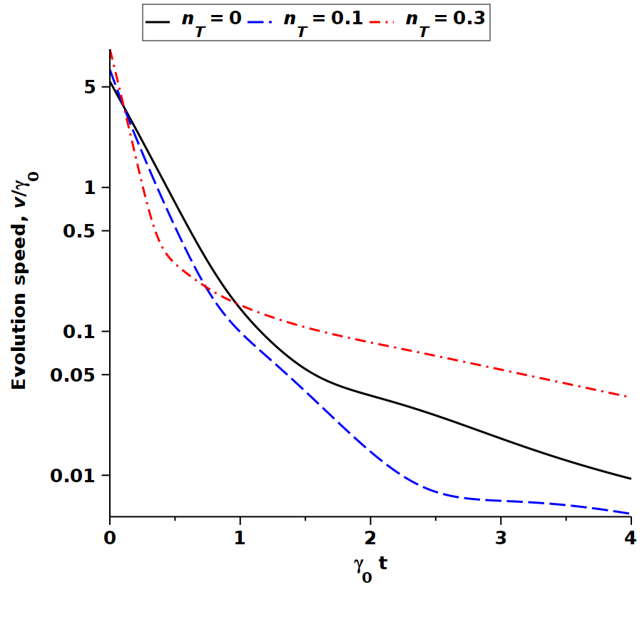
(b) $\theta_{\Gamma}=\pi/4$

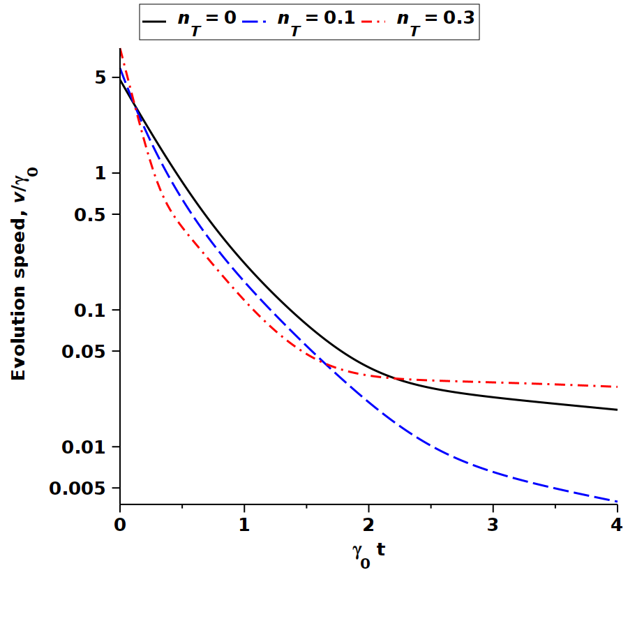
(c) $\theta_{\Gamma}=0$

Figure 1: Speed of evolution computed from Eq. (106) for the initial state (108) with $\theta=\pi/4$ and $\phi=0$ as a function of the dimensionless time parameter, $\gamma_{0}t$, at the frequency and relaxation vectors: $\bm{\omega}=0.9\gamma_{0}(0,0,1)$ and $\bm{\gamma}=0.9\gamma_{0}(\sin\theta_{\Gamma},0,\cos\theta_{\Gamma})$. Three cases are shown: (a) $\theta_{\Gamma}=\pi/2$, (b) $\theta_{\Gamma}=\pi/4$ and (c) $\theta_{\Gamma}=0$. Solid, dashed and dotted-dashed lines are evaluated at $n_{T}=0$, $n_{T}=0.1$ and $n_{T}=0.3$, respectively.

In this section, our starting point is the Hilbert-Schmidt metric expression for the speed of evolution [73]:

$$v(t)=\sqrt{\text{Tr}\Big{(}\Bigl{[}\frac{\partial}{\partial t}\hat{\rho}(t)\Bigr{]}^{2}\Big{)}}\equiv\Bigl{\|}\frac{\partial\hat{\rho}(t)}{\partial t}\Bigr{\|}_{2}$$

$$=\sqrt{\text{Tr}\Big{(}\Bigl{[}\hat{\mathcal{L}}e^{\hat{\mathcal{L}}t}\hat{\rho}(0)\Bigr{]}^{2}\Big{)}},$$ (100)

where we have used the relation: $\hat{\rho}(t)=e^{\hat{\mathcal{L}}t}\hat{\rho}(0)$. For instance, when the system is initially prepared in the pure state with $\hat{\rho}(0)=\left|\psi_{0}\right>\left<\psi_{0}\right|$, this speed determines the upper bound for the rate of change of the fidelity [79, 80]:

$$\left|\frac{\partial}{\partial t}\left<\psi_{0}\right|\hat{\rho}(t)\left|\psi_{0}\right>\right|\leq v(t).$$ (101)

Note that a similar result applies to the rate of the Hilbert-Schmidt distance $\|\hat{\rho}(t)-\hat{\rho}(0)\|_{2}$ between the initial and the evolved states.

Dynamical behavior of the evolution speed (100) is determined by both the spectrum of the Liouvillian and the initial state $\hat{\rho}(0)$. In the linear approximation, the expression for the product of superoperators that enter Eq. (100)

$$\hat{\mathcal{L}}e^{\hat{\mathcal{L}}t}\approx$$

$$\approx e^{-\hat{\mathcal{K}}^{(-)}_{I}}\Bigl{\{}\hat{\mathcal{L}}_{d}+n_{T}(\hat{\mathcal{K}}^{(+)}_{\Gamma}+\hat{\mathcal{L}}_{d}\hat{\mathcal{K}}^{(+)}_{W(t)})\Bigr{\}}e^{\hat{\mathcal{L}}_{d}t}e^{\hat{\mathcal{K}}^{(-)}_{I}}$$ (102)

can be obtained using Eqs. (92) and (99) (for more technical details see Appendix B). An important point is that the approximated superoperator (IV.3) maps density operators which are finite dimensional in the Fock basis into finite dimensional ones.

In the limiting case of zero-temperature environment with $n_{T}=0$, the squared evolution speed is given by

$$v_{0}^{2}(t)=\mathop{\rm Tr}\nolimits\Bigl{\{}(\hat{\mathcal{L}}_{0}\hat{\rho}_{0}(t))^{2}\Bigr{\}}\equiv\text{Tr}\Bigl{\{}(\hat{v}_{0}(t))^{2}\Bigr{\}}$$

$$=\text{Tr}\Bigl{\{}(e^{-\hat{\mathcal{K}}^{(-)}_{I}}\hat{\mathcal{L}}_{d}e^{\hat{\mathcal{L}}_{d}t}e^{\hat{\mathcal{K}}^{(-)}_{I}}\hat{\rho}(0))^{2}\Bigr{\}},$$ (103)

where

$$\hat{\rho}_{0}(t)=e^{\hat{\mathcal{L}}_{0}t}\hat{\rho}(0),\quad\hat{v}_{0}\equiv\frac{\partial\hat{\rho}_{0}}{\partial t}.$$ (104)

When $\hat{\rho}(0)$ is the statistical operator with the finite dimensional support in the Fock basis, the superoperator $e^{-\hat{\mathcal{K}}^{(-)}_{I}}\hat{\mathcal{L}}_{d}e^{\hat{\mathcal{L}}_{d}t}e^{\hat{\mathcal{K}}^{(-)}_{I}}$ keeps the support dimension finite and computing of the squared evolution speed does not require using sophisticated tools.

We can now use the approximate formula Eq. (IV.3) to study the effect of thermal photons on the evolution speed in the first-order (linear) approximation. According to Eq. (IV.2), in this approximation, the density matrix can be written in the form

$$\hat{\rho}(t)\approx\hat{\rho}_{0}(t)+n_{T}\hat{\rho}_{1}(t),\quad\hat{\rho}_{1}(t)=\hat{U}_{1}(t)\rho_{0}(t),$$ (105)

where the superoperator $\hat{U}_{1}(t)$ given by Eq. (97) acts on the zero-temperature density matrix, $\hat{\rho}_{0}$, producing the first order correction, $\hat{\rho}_{1}$. The resulting expression for the squared speed of evolution reads

$$v^{2}(t)\approx\mathop{\rm Tr}\nolimits((\hat{v}_{0}+n_{T}\hat{v}_{1})^{2}),\quad\hat{v}_{1}\equiv\frac{\partial\hat{\rho}_{1}}{\partial t}.$$ (106)

Approximate relations (IV.3) and (106) can now be applied to the special case of the two-mode system introduced in Sec. IV.1. To be specific, it will be assumed that the system represents the quantum polarization states, where $\hat{a}_{1}\equiv\hat{a}_{H}$ and $\hat{a}_{2}\equiv\hat{a}_{V}$ are the annihilation operators for horizontally and vertically polarized photon modes, respectively, and the initial state is a pure single-photon state taken in the form:

$$\hat{\rho}(0)=\left|\psi_{0}\right>\left<\psi_{0}\right|,$$

$$\left|\psi_{0}\right>=\cos\frac{\theta}{2}\left|1_{H},0_{V}\right>+e^{i\phi}\sin\frac{\theta}{2}\left|0_{H},1_{V}\right>$$ (107)

where $\left|n_{H},m_{V}\right>\equiv\left|n_{H}\right>\otimes\left|m_{V}\right>$. This is the state of polarization qubit which, at $\phi=0$, is linearly polarized along the unit vector, $(\cos\theta,\sin\theta,0)$, specified by the polarization azimuth $\theta$. The initial density matrix can be rewritten using the superoperators $\hat{\mathcal{K}}^{(+)}_{mn}$ as follows

$$\hat{\rho}(0)=\hat{\mathcal{K}}^{(+)}_{R_{0}}\left|\mathbf{0}\right>\left<\mathbf{0}\right|,\quad R_{0}=\frac{1}{2}\left\{\sigma_{0}+(\mathbf{n},\bm{\sigma})\right\}$$ (108)

where $\mathbf{n}=(\sin\theta\cos\phi,\sin\theta\sin\phi,\cos\theta)$ and $\left|\mathbf{0}\right>\equiv\left|0_{H},0_{V}\right>$ is the vacuum state.

(a) $n_{T}=0,\>\theta_{\Gamma}=\pi/2$

(b) $n_{T}=0.3,\>\theta_{\Gamma}=\pi/2$

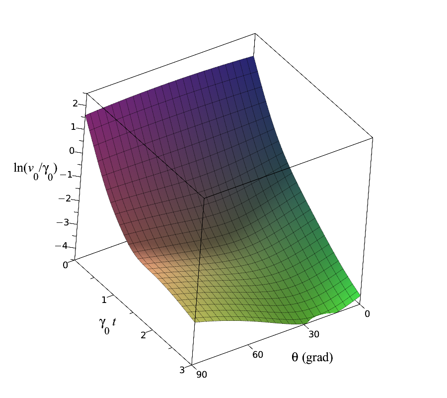
(c) $n_{T}=0,\>\theta_{\Gamma}=\pi/4$

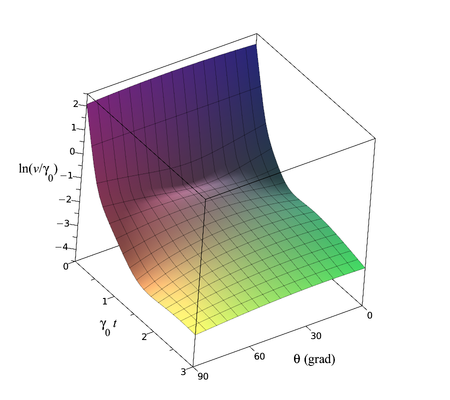
(d) $n_{T}=0.3,\>\theta_{\Gamma}=\pi/4$

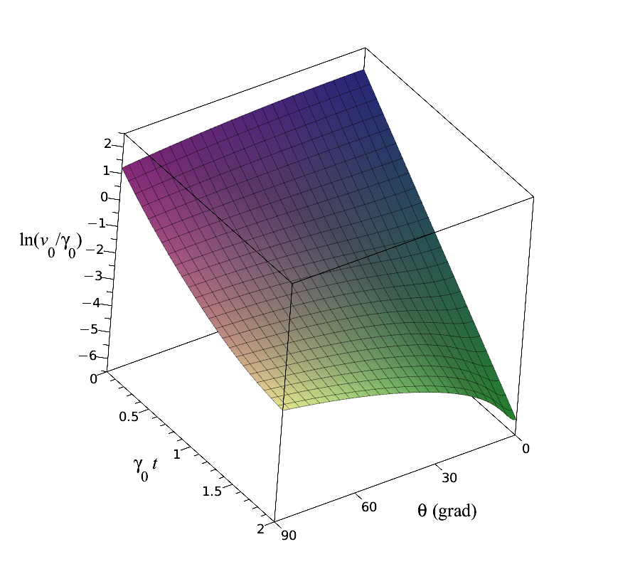
(e) $n_{T}=0,\>\theta_{\Gamma}=0$

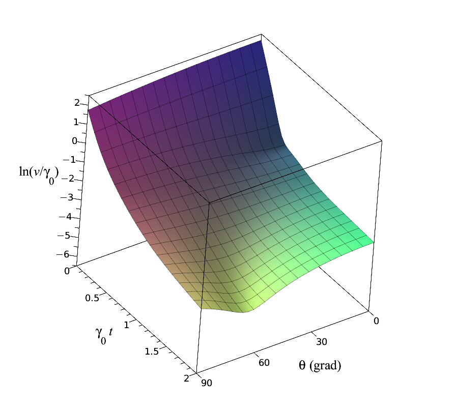
(f) $n_{T}=0.3,\>\theta_{\Gamma}=0$

Figure 2: Speed of evolution in the $\gamma_{0}t$–$\theta$ plane computed for the polarization qubit states (IV.3) with $\phi=0$ at various values of $n_{T}$ and $\theta_{\Gamma}$: (a) $n_{T}=0$ and $\theta_{\Gamma}=\pi/2$; (b) $n_{T}=0.3$ and $\theta_{\Gamma}=\pi/2$; (c) $n_{T}=0$ and $\theta_{\Gamma}=\pi/4$; (d) $n_{T}=0.3$ and $\theta_{\Gamma}=\pi/4$; (e) $n_{T}=0$ and $\theta_{\Gamma}=0$; (f) $n_{T}=0.3$ and $\theta_{\Gamma}=0$. The frequency and relaxation vectors are $\bm{\omega}=0.9\gamma_{0}(0,0,1)$ and $\bm{\gamma}=0.9\gamma_{0}(\sin\theta_{\Gamma},0,\cos\theta_{\Gamma})$, respectively.

Time-dependent part of Eqs. (IV.3) and (106) is determined by the zero-temperature density matrix $\hat{\rho}_{0}(t)=e^{\hat{\mathcal{L}}_{0}t}\rho(0)$. For the initial state (108), the expression for this matrix

$$\hat{\rho}_{0}(t)=(\hat{\mathcal{K}}^{(+)}_{R}+r)\left|\mathbf{0}\right>\left<\mathbf{0}\right|,$$ (109)

$$R=P(t)R_{0}{P}^{\dagger}(t),\>r=1-\mathop{\rm Tr}\nolimits R$$ (110)

can be deduced with the help of the identities (B) –(140) derived in Appendix B.

From Eq. (B) giving the derivative of $\hat{\rho}_{0}$ with respect time

$$\hat{v}_{0}\equiv\frac{\partial\hat{\rho}_{0}}{\partial t}=(\hat{\mathcal{K}}^{(+)}_{\dot{R}}+\dot{r})\left|\mathbf{0}\right>\left<\mathbf{0}\right|,$$ (111)

where dot stands for derivative with respect time, it is not difficult to express the zero-temperature speed of evolution in terms of the matrix $R$ as follows (see also Eq. (142) in Appendix B):

$$v_{0}^{2}=\mathop{\rm Tr}\nolimits\hat{v}_{0}^{2}=\mathop{\rm Tr}\nolimits\dot{R}^{2}+\dot{r}^{2},$$ (112)

where

$$\dot{r}=-\mathop{\rm Tr}\nolimits\dot{R},\quad\dot{R}=P(t)R_{1}{P}^{\dagger}(t),$$ (113a)

$$R_{1}=LR_{0}+R_{0}{L}^{\dagger}=-[\gamma_{0}+(\bm{\gamma},\mathbf{n})]\sigma_{0}$$

$$+(\bm{\omega}\times\mathbf{n}-\bm{\gamma}-\gamma_{0}\mathbf{n},\bm{\sigma}).$$ (113b)

(a) $\omega=0$

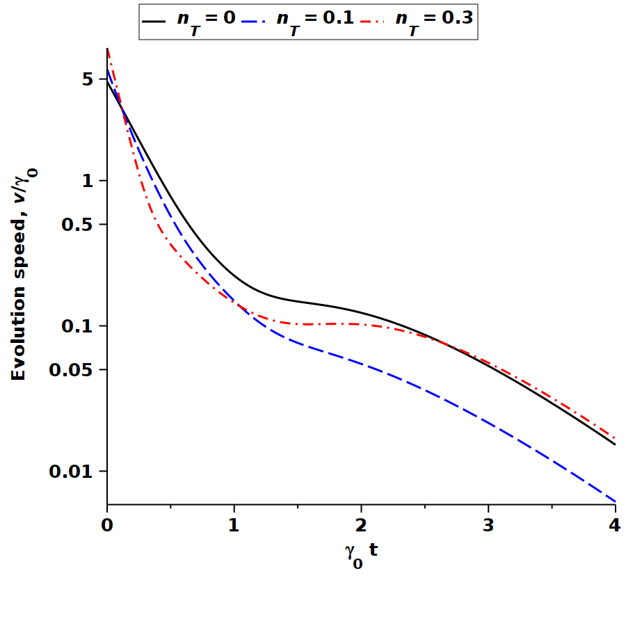
(b) $\omega=\gamma$

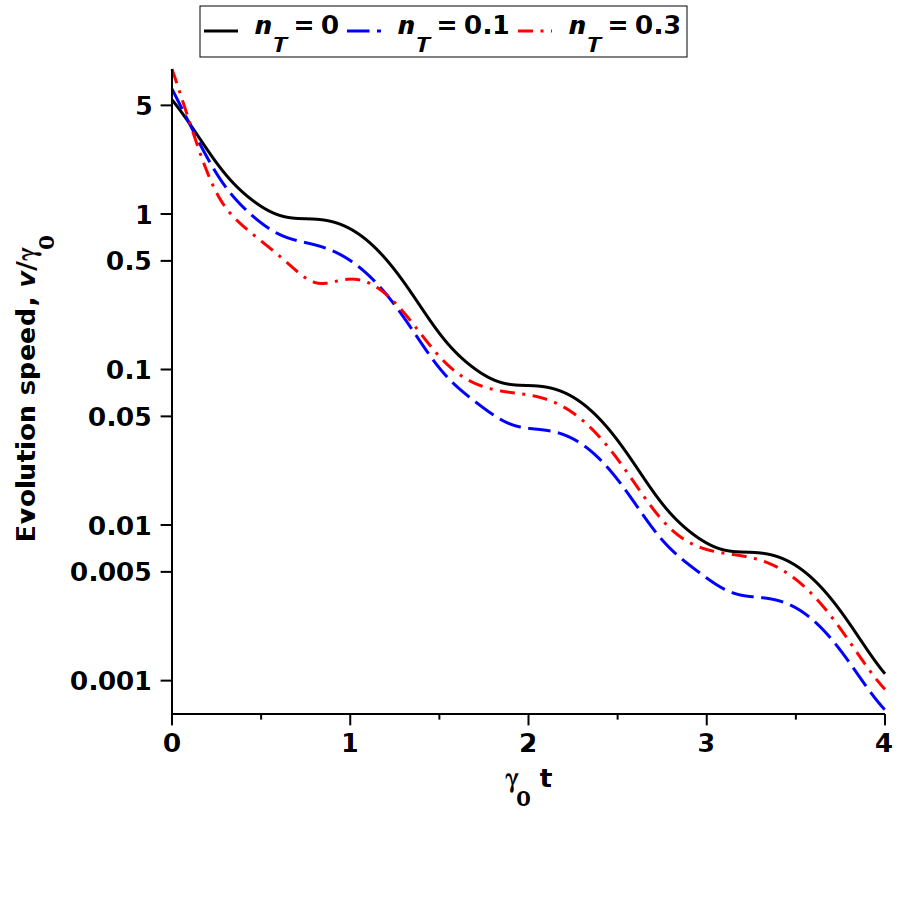
(c) $\omega=3\gamma$

Figure 3: Time dependence of evolution speed for the polarization qubit state (IV.3) with $\theta=\pi/4$ and $\phi=0$. The frequency and relaxation vectors are $\bm{\omega}=(0,0,\omega)$ and $\bm{\gamma}=(0.9\gamma_{0},0,0)$, respectively. Three cases are shown: (a) $\omega=0$, (b) $\omega=\gamma$ and (c) $\omega=3\gamma$. Solid, dashed and dotted-dashed lines are evaluated at $n_{T}=0$, $n_{T}=0.1$ and $n_{T}=0.3$, respectively.

The latter can be calculated using the identities (B) and the commutation relations (21). The result reads

$$\hat{\rho}_{1}(t)=(\hat{\mathcal{K}}^{(+)}_{W}\hat{\mathcal{K}}^{(+)}_{R}+\hat{\mathcal{K}}^{(+)}_{V}+v)\left|\mathbf{0}\right>\left<\mathbf{0}\right|,$$ (114)

where

$$V=W-W\mathop{\rm Tr}\nolimits R-R\mathop{\rm Tr}\nolimits W-\{R,W\},$$ (115a)

$$v=\mathop{\rm Tr}\nolimits(RW)+\mathop{\rm Tr}\nolimits R\mathop{\rm Tr}\nolimits W-\mathop{\rm Tr}\nolimits W.$$ (115b)

Now it is rather straightforward to obtain the expression for the first-order correction operator, $\hat{v}_{1}$, that enters the evolution speed (106) given by

$$\hat{v}_{1}\equiv\frac{\partial\hat{\rho}_{1}}{\partial t}=\bigl{(}\hat{\mathcal{K}}^{(+)}_{\dot{W}}\hat{\mathcal{K}}^{(+)}_{R}+\hat{\mathcal{K}}^{(+)}_{W}\hat{\mathcal{K}}^{(+)}_{\dot{R}}$$

$$+\hat{\mathcal{K}}^{(+)}_{\dot{V}}+\dot{v}\bigr{)}\left|\mathbf{0}\right>\left<\mathbf{0}\right|,$$ (116)

where $\dot{V}$ is the time derivative of the matrix (115a) that, in addition to $R$ and $W$, depends on $\dot{R}$ (see Eq. (113)) and $\dot{W}=-\dot{Q}=P(t)\Gamma{P}^{\dagger}(t)$ with $\Gamma=2[\gamma_{0}\sigma_{0}+(\bm{\gamma},\bm{\sigma})]$.

Note that the above algebraic considerations leading to formulas (112)–(IV.3) are based on the linear approximation for the superpropagator given by Eq. (99). Alternative algebraic calculations with Eqs. (IV.3) and (106) serving as the starting points are detailed in Appendix B (see Eqs. (B) –(B)).

These formulas can be conveniently used for numerical analysis of the evolution speed that involves evaluation of the matrices $P(t)$ as one of the most important steps. Equation (IV.1) gives the matrix $P(t)$ expressed in terms of the frequency and relaxation rate vectors, $\bm{\omega}$ and $\bm{\gamma}$, describing the matrices, $\Omega$ and $\Gamma/2$, in the basis of the Pauli matrices. In our subsequent calculations, we shall utilize the angular parametrization of these vectors given by Eq. (IV.1) and, without loss of generality, assume that the frequency matrix is diagonal: $\bm{\omega}=(0,0,\omega)$.

Note that, from Eq. (IV.1), the matrices $R$ (see Eq. (110)) and $W$ (see Eq. (98)) are both independent of the frequency $\omega_{0}$. Therefore, this frequency has no effect on the evolution speed (106).

In Figure 1, the semi-log plots present the numerical results for time dependencies of the dimensionless evolution speed $v/\gamma_{0}$ computed at $\omega/\gamma_{0}=\gamma/\gamma_{0}=0.9$ with different values of the thermal photon mean number $n_{T}\in\{0,0.1,0.3\}$ and of the angle $\theta_{\Gamma}\in\{\pi/2,\pi/4,0\}$ between the frequency vector $\mathbf{n}_{\Omega}=(0,0,1)$ and the relaxation vector $\mathbf{n}_{\Gamma}=(\sin\theta_{\Gamma},0,\cos\theta_{\Gamma})$.

Referring to Fig. 1, it can be seen that all the curves are approaching zero in the long time limit, where the density matrix reaches the thermal equilibrium state. Another effect is that, at elevated temperatures with $n_{T}=0.1$ and $n_{T}=0.3$, the initial value of the evolution speed $v(0)$ increases as compared to the zero-temperature case with $n_{T}=0$. At the same time, the rate of the initial evolution speed decay is accelerated with temperature.

Figure 2 shows the evolution speed surfaces in the $\gamma_{0}t$–$\theta$ plane evaluated at different values of temperature and the angle $\theta_{\Gamma}$. It is demonstrated that, in addition to the temperature and the angle between the coherent and incoherent coupling vectors, $\bm{\omega}$ and $\bm{\gamma}$, the evolution speed dynamics depends on the unit vector $\mathbf{n}$ that specifies the initial state of the polarization qubit (108). More specifically, from Fig. 2, it may be seen that the speed versus time curves appear to be sensitive to the orientation of the linear polarization axis: $(\sin\theta,\cos\theta,0)$.

For instance, Figures 2(e) and 2(f) present the results for the simplest case, where $\bm{\omega}=\bm{\gamma}\parallel(0,0,1)$ and the matrix ${P}^{\dagger}(t)P(t)=\mathrm{e}^{-2\gamma_{0}t}\mathop{\rm diag}\nolimits(\mathrm{e}^{-2\gamma t},\mathrm{e}^{2\gamma t})$ is diagonal. As is shown in Fig. 2(e), at $n_{T}=0$ and $\theta=0$, we have the regime of fast perfectly single-exponential relaxation, where $v_{0}\propto\mathrm{e}^{-2(\gamma_{0}+\gamma)t}$. This regime changes with $\theta$ and the relaxation slows down due to growing contribution of the terms proportional to $\mathrm{e}^{-2(\gamma_{0}-\gamma)t}$. Referring to Fig. 2(f), at non-zero temperature, the dynamics is complicated by additional products of fast and slow exponential functions coming from the first-order correction (IV.3). Similar remarks apply to the surfaces 2(a)–2(d) with non-vanishing angle between $\bm{\omega}$ and $\bm{\gamma}$.

Figure 3 shows the speed of evolution computed as a function of time parameter, $\gamma_{0}t$, at different values of the frequency, $\omega$, assuming that the dynamical coupling (frequency) vector $\bm{\omega}=(0,0,\omega)$ is normal to the incoherent coupling (relaxation) vector $\bm{\gamma}=(\gamma,0,0)$. As is illustrated in Fig. 3, the exceptional point that takes place at $\omega=\gamma$ (see Fig. 3(b)) separates two qualitatively different dynamical regimes. These regimes are determined by the parameter $q$ (see Eq. (89)) that enters the matrix $P(t)$ (see Eq. (IV.1)): (a) the exponential regime (see Fig. 3(a)) corresponds to the case, where $\omega$ is smaller than $\gamma$ and the parameter $q$ is real; (b) the oscillatory regime (see Fig. 3(c)) occurs when $\omega$ exceeds $\gamma$ so that the value of $q$ is imaginary.

V Conclusions and discussion

In this paper, we have studied Lindblad dynamics of the multimode bosonic system interacting with the thermal environment governed by the GKSL equation (3) that involves both coherent (dynamical) and incoherent (environment mediated) intermode couplings represented by the frequency and the relaxation matrices: $\Omega$ and $\Gamma$, respectively. At the heart of our general approach to the dynamics is the Lie algebra of quadratic combinations of the left and right superoperators (see Eqs. (4a)–(4c)), $\{\overleftarrow{\hat{a}^{\dagger}_{i}},\overleftarrow{\hat{a}_{i}}\}_{i=1}^{N}$ and $\{\overrightarrow{\hat{a}^{\dagger}_{i}},\overrightarrow{\hat{a}_{i}}\}_{i=1}^{N}$, with the commutation relations given by Eq. (20).

We have found that introducing the superoperators associated with matrices (see Sec. II.3 and the commutation relations (21)) leads to a natural representation of the algebraic structure of the Liouvillian (see Eq. (17)) and significantly simplifies analysis of this algebra. This step can be regarded as an extension of the well-known Jordan-Schwinger approach outlined in Sec. II.2 to the case of superoperators.

We have derived the algebraic identities (22) which are utilized to transform the Liouvillian into the so-called diagonalized form (24) (the form where the contributions coming from the jump superoperators $\hat{\mathcal{K}}^{(\pm)}$ are eliminated) using the differently ordered superoperators given by Eqs. (25) and (26). According to formulas (III.1) and (III.1) describing results for the Liouvillian, $\hat{\mathcal{L}}$, and its conjugate, $\hat{\mathcal{L}}^{\sharp}$, defined using relation (19), the diagonalized Liouvillian is completely determined by the effective non-Hermitian Hamiltonian (III.1), $\hat{H}_{\mathrm{eff}}$, associated with the matrix $H=\Omega-i\Gamma/2$ through the Jordan mapping (7). By contrast to the approximate semiclassical Hamiltonian (II.1), the effective Hamiltonian is temperature independent and the associated matrix $H$ governs both the spectral properties of the Liouvillian and the regimes of Lindblad dynamics. In particular, at Liouvillian exceptional points, this matrix cannot be diagonalized.

We have expressed the spectrum and eigenoperators of the Liouvillian, $\hat{\mathcal{L}}$, in terms of the eigenvalues and the eigenstates of the operator proportional to the Hamiltonian, $\hat{L}_{\mathrm{eff}}=-i\hat{H}_{\mathrm{eff}}$ (see Eqs. (49)–(54)). Efficiency of the method is demonstrated by solving the spectral problem (see Eqs. (III.2)–(60)) and deriving the eigenmode decomposition of the matrix density evolved in time (see Eqs. (61)–(66)) for the single-mode Liouvillian closely related to the case of non-interacting modes. Note that, in Appendix A, we have employed the method of generating operators as a tool that considerably simplifies derivation of the biorthogonality relations.

For the case where the matrix $H$ is diagonalizable, we have shown how to diagonalize the effective Hamiltonian, solve the spectral problem and obtain the eigenmode expansion for $\hat{\rho}(t)$ (see Eqs. (III.2)–(76)). We have also derived an alternative representation for $\hat{\rho}(t)$ that remains valid even if the matrix $H$ is non-diagonalizable (see Eqs. (III.2)–(76)). The latter is the case that occurs when a Liouvillian exceptional point comes into play.

General theoretical results are illustrated by applications related to the dynamics of photonic polarization modes represented by a two-mode bosonic system. In this case, the matrices $\Omega$ and $\Gamma$ expressed in terms of in of the Pauli matrices are conveniently parameterized by the frequency and relaxation vectors, $\bm{\omega}$ and $\bm{\gamma}$ (see Eq. (IV.1)).

The explicit expression for the matrix exponential $P(t)=e^{-iHt}$ given by Eq. (IV.1) shows that the dynamical regimes are governed by the parameter $q$ (see Eq. (89)) that determines the eigenvalues of the matrix $iH$: $\lambda_{\pm}=i\omega_{0}+\gamma_{0}\pm q$. Formula (IV.1) is used to deduce two relations (90) describing the geometry of $\bm{\omega}$ and $\bm{\gamma}$ at EPs, where the parameter $q$ vanishes along with the difference between the above eigenvalues: $|\bm{\omega}|\equiv\omega=|\bm{\gamma}|\equiv\gamma$ and $\bm{\omega}\perp\bm{\gamma}$.

When Eq. (IV.1) is compared with its EP limit (91), it is apparent that EPs would manifest themselves in the effect of EP induced slowdown. In the special case where $\bm{\omega}$ is aligned perpendicular to $\bm{\gamma}$, EP represents the point separating the regions with $\omega>\gamma$ (the value of $q$ is imaginary) and $\omega<\gamma$ ($q$ is real-valued). So, we have two different dynamical regimes separated by the EP. A similar result was reported in Ref. [73] for a simple model represented by the qubit system with the Hamiltonian and the jump operator taken to be proportional to the Pauli matrices $\sigma_{1}$ and $\sigma_{3}$, respectively. Note that this qubit model can be transformed into the spin-1/2 model studied in Ref. [83] where the above matrices $\sigma_{1}$ and $\sigma_{3}$ are interchanged. A more complicated example of a two-level system with EPs and the jump operators describing three different decoherence channels was recently reported in [84].

In order to study the speed of evolution in the low-temperature regime, where the mean number of thermal photons $n_{T}$ is small, we have deduced approximate expressions for the Liouvillian, $\hat{\mathcal{L}}$, and the superpropagator, $e^{\hat{\mathcal{L}}t}$, that linearly depend on $n_{T}$ (see Eqs. (IV.2) and (99)). These formulas lead to the approximate density matrix (105) and the speed of evolution (106) utilized to perform numerical analysis for the single-photon initial state (IV.3) described by the density matrix of the polarization qubit (108). (At $\phi=0$, the qubit is linearly polarized with the polarization azimuth $\theta$.)

In order to evaluate the evolution speed (106), we have derived the analytical formulas for the zero-temperature density matrix (109) and the first-order correction (114) defined with the help of the superoperators $\hat{\mathcal{K}}^{(+)}_{mn}$ associated with the time-dependent matrices $W$ (see Eq. (98)), $R$ (see Eq. (110)) and $V$ (see Eq. (115a)). Interestingly, these formulas can be used to demonstrate the difference between the polarization qubit dynamics and temporal evolution of atomic two-level systems that interact with a bosonic bath and the jump operators are proportional to $\sigma_{\pm}=(\sigma_{1}\pm i\sigma_{2})/2$ (see, for instance, equation (2.19) in Ref. [65]).

In addition, our general results for zero-temperature dynamics of Fock states provide a useful tool for analysis of generalized models of passive parity-time-symmetric optical directional couplers dealing with two-mode bosonic systems that represent the light traveling along evanescently coupled waveguides [85, 86].

The curves depicted in Fig. 1 illustrate temperature induced effects in dynamics of the evolution speed. Specifically, the initial evolution speed is found to increase with temperature and it decays more rapidly at short times as the temperature goes up. For linearly polarized qubit (IV.3) with vanishing $\phi$, the evolution speed surfaces depicted in Fig. 2 demonstrate sensitivity of the dynamics to orientation of polarization axis specified by the polarization azimuth $\theta$ In Fig. 3, we have also evaluated the evolution speed at $\bm{\omega}=(0,0,\omega)$ normal to $\bm{\gamma}=(\gamma,0,0)$ to visualize two qualitatively different dynamical regimes with $\omega<\gamma$ and $\omega>\gamma$ separated by the EP at $\omega=\gamma$.

The peculiarity of the low-temperature approximation with the Liouvillian and the superpropagator expanded as power series in $n_{T}$ is that the corresponding approximate superoperators acting on density matrices with finite dimensional support in the Fock basis will produce the operators whose support is also finite dimensional. Thus, by using this approximation, theoretical treatment of the Lindblad dynamics of such states that exemplify extremes opposite to the well-known Gaussian states can be performed within the realm of finite dimensional models.

Our results are applicable to bosonic systems with arbitrary number of modes, so it is rather straightforward to go beyond the limitations of the two-mode system by taking into consideration additional modes. For instance, such generalizations will be useful when studying the dynamics of light in such systems as twisted fibers [87] and open resonators with overlapping modes [45]. Among a wide range of potential applications, note that our method provides an efficient tool for computing multiple-time correlation functions using the quantum regression theorem (a recent discussion of related techniques can be found in Refs. [88, 89]).

Appendix A Generating operators and biorthogonality relations

In this Appendix, we derive the biorthogonality relations for the eigenoperators of the single-mode Liouvillian $\hat{\mathcal{L}}$ and its adjoint $\hat{\mathcal{L}}^{\sharp}$: $\hat{\rho}_{mn}$ and $\hat{\sigma}_{nm}$ given by Eqs. (59) and (III.2), respectively.

To this end, we introduce the generating operators

$$\hat{\rho}(\alpha,\alpha^{\ast})=\sum_{m,n=0}^{\infty}\frac{\hat{\rho}_{mn}}{\sqrt{m!n!}}\alpha^{m}(-\alpha^{\ast})^{n}$$

$$=e^{Z|\alpha|^{2}}e^{\alpha\hat{a}^{\dagger}}\hat{\rho}_{0}e^{-\alpha^{\ast}\hat{a}},$$ (117)

$$\hat{\sigma}(\beta,\beta^{\ast})=\sum_{m,n=0}^{\infty}\frac{\hat{\sigma}_{nm}}{\sqrt{n!m!}}\beta^{n}(-\beta^{\ast})^{m}$$

$$=e^{n_{T}|\beta|^{2}}e^{\beta\hat{a}^{\dagger}}e^{-\beta^{\ast}\hat{a}}$$ (118)

that can be computed using the explicit expressions for $\hat{\rho}_{mn}$ and $\hat{\sigma}_{nm}$ (see Eqs. (59) and (III.2)).

Our next step is to use the identity

$$\mathrm{Tr}[(\hat{a}^{\dagger})^{n}\hat{\rho}_{0}(\hat{a})^{m}]=n!Z^{n+1}\delta_{nm},$$ (119)

that can be obtained by integrating the Husimi symbol (the $Q$-symbol) of the normally ordered operator (see normally ordered expression for $\hat{\rho}_{0}$ given in Eq. (60)), for derivation of the following relation:

$$\mathrm{Tr}[e^{\alpha\hat{a}^{\dagger}}\hat{\rho}_{0}e^{-\alpha^{\ast}\hat{a}}]=Ze^{-Z|\alpha|^{2}}.$$ (120)

This relation can now be combined with the formula

$$e^{\beta\hat{a}^{\dagger}}e^{-\beta^{\ast}\hat{a}}=e^{|\beta|^{2}}e^{-\beta^{\ast}\hat{a}}e^{\beta\hat{a}^{\dagger}}$$ (121)

linking normally and antinormally ordered products of the exponentials that enter the generating operator (A) to deduce our key analytical result

$$\mathrm{Tr}[\hat{\sigma}(\beta,\beta^{\ast})(\hat{\rho}(\alpha,\alpha^{\ast})]=Ze^{-Z(\alpha\beta^{\ast}+\alpha^{\ast}\beta)}.$$ (122)

A comparison between power series expansions for the left- and right-hand sides of Eq. (122) immediately leads to the biorthogonality relations of the form:

$$\mathrm{Tr}[\hat{\sigma}_{nm}\hat{\rho}_{m^{\prime}n^{\prime}}]=\delta_{nn^{\prime}}\delta_{mm^{\prime}}Z^{n+m+1}.$$ (123)

Appendix B Superoperator of evolution in linear approximation

In this Appendix, we shall detail calculations related to the low-temperature regime where the mean photon number $n_{T}$ is small. In this regime, the Liouvillian and the superpropagator can be approximated by a sum of their zero-temperature expressions and the first-order corrections, which are linear in $n_{T}$. Formulas (IV.2)–(94) give the linear approximation for the Liouvillian, whereas the result for the superpropagator (IV.2) is expressed in terms of the operator $\hat{U}_{1}(t)$ defined in Eq. (96).

In order to deduce the expression for $\hat{U}_{1}(t)$ given by Eq. (97), we cast the time-dependent term on the right-hand side of Eq. (96) into the form:

$$e^{\hat{\mathcal{L}}_{0}t}(\hat{\mathcal{K}}^{(+)}_{I}-\hat{\mathcal{K}}^{(-)}_{I})e^{-\hat{\mathcal{L}}_{0}t}$$

$$=e^{-\hat{\mathcal{K}}^{(-)}_{I}}e^{\hat{\mathcal{L}}_{d}t}e^{\hat{\mathcal{K}}^{(-)}_{I}}(\hat{\mathcal{K}}^{(+)}_{I}-\hat{\mathcal{K}}^{(-)}_{I})e^{-\hat{\mathcal{K}}^{(-)}_{I}}e^{-\hat{\mathcal{L}}_{d}t}e^{\hat{\mathcal{K}}^{(-)}_{I}}$$

$$=e^{-\hat{\mathcal{K}}^{(-)}_{I}}e^{\hat{\mathcal{L}}_{d}t}(\hat{\mathcal{K}}^{(+)}_{I}+2\hat{\mathcal{K}}^{(0)}_{I})e^{-\hat{\mathcal{L}}_{d}t}e^{\hat{\mathcal{K}}^{(-)}_{I}},$$ (124)

time dependence is governed by the diagonalized superpropagator $e^{\hat{\mathcal{L}}_{d}t}$.

Our next step utilizes the algebraic identity (see Eq. (III.2) for a similar result used to diagonalize the effective Hamiltonian)

$$e^{\overleftarrow{\hat{V}_{+}}+\overrightarrow{\hat{V}_{-}}}\{\overleftarrow{\hat{A}_{+}}\overrightarrow{\hat{A}_{-}}\}e^{-\overleftarrow{\hat{V}_{+}}-\overrightarrow{\hat{V}_{-}}}=\overleftarrow{\hat{A}_{+}^{\prime}}\overrightarrow{\hat{A}_{-}^{\prime}},$$

$$\hat{A}_{\pm}^{\prime}=e^{\pm\hat{V}_{\pm}}\hat{A}_{\pm}e^{\mp\hat{V}_{\pm}}$$ (125)

with $\hat{V}_{+}=\hat{V}_{-}^{\dagger}=\hat{L}_{\mathrm{eff}}t=\hat{J}_{L}t$. By using this identity and Eq. (10) we can simplify the operators that enter Eq. (B) as follows

$$e^{\hat{\mathcal{L}}_{d}t}\hat{\mathcal{K}}^{(0)}_{I}e^{-\hat{\mathcal{L}}_{d}t}=\hat{\mathcal{K}}^{(0)}_{I}$$ (126)

$$e^{\hat{\mathcal{L}}_{d}t}\hat{\mathcal{K}}^{(+)}_{I}e^{-\hat{\mathcal{L}}_{d}t}=\hat{\mathcal{K}}^{(+)}_{Q(t)},$$ (127)

where $Q(t)=P(t)P^{\dagger}(t)=e^{Lt}e^{L^{\dagger}t}$. For the two-mode systems, the closed-form expression for $Q(t)$ can be easily computed from Eq. (IV.1).

We can now substitute the relations

$$e^{-\hat{\mathcal{K}}^{(-)}_{I}}\hat{\mathcal{K}}^{(+)}_{Q(t)}e^{\hat{\mathcal{K}}^{(-)}_{I}}=\hat{\mathcal{K}}^{(+)}_{Q(t)}-2\hat{\mathcal{K}}^{(0)}_{Q(t)}+\hat{\mathcal{K}}^{(-)}_{Q(t)},$$ (128)

$$e^{-\hat{\mathcal{K}}^{(-)}_{I}}\hat{\mathcal{K}}^{(0)}_{I}e^{\hat{\mathcal{K}}^{(-)}_{I}}=\hat{\mathcal{K}}^{(0)}_{I}-\hat{\mathcal{K}}^{(-)}_{I}$$ (129)

along with Eqs. (126)-(127) into Eq. (B) to deduce the result leading to Eq. (97).

In order to obtain higher order corrections and go beyond the linear approximation, we have to consider the following commutation relations

$$[\hat{\mathcal{K}}^{(s)}_{A},e^{\hat{\mathcal{L}}^{(d)}t}]=\big{(}\hat{\mathcal{K}}^{(s)}_{A}+e^{\hat{\mathcal{L}}^{(d)}t}\hat{\mathcal{K}}^{(s)}_{A}e^{-\hat{\mathcal{L}}^{(d)}t}\big{)}e^{\hat{\mathcal{L}}^{(d)}t},$$ (130)

where $s\in\{0,\pm\}$ and $A$ is an arbitrary matrix. Similar to Eq. (126)–(127), derivation of the closed-form expressions for $e^{\hat{\mathcal{L}}^{(d)}t}\hat{\mathcal{K}}^{(\pm)}_{A}e^{-\hat{\mathcal{L}}^{(d)}t}$:

$$e^{\hat{\mathcal{L}}_{d}t}\hat{\mathcal{K}}^{(+)}_{A}e^{-\hat{\mathcal{L}}_{d}t}=\hat{\mathcal{K}}^{(+)}_{e^{Lt}Ae^{L^{\dagger}t}},$$ (131)

$$e^{\hat{\mathcal{L}}_{d}t}\hat{\mathcal{K}}^{(-)}_{A}e^{-\hat{\mathcal{L}}_{d}t}=\hat{\mathcal{K}}^{(-)}_{e^{-L^{\dagger}t}Ae^{e^{-Lt}}}$$ (132)

uses Eqs. (B) and (III.2) in combination with the identities (9)–(10). Note that Eq. (131) leads to the commutation relation

$$[\hat{\mathcal{L}}_{d},\hat{\mathcal{K}}^{(+)}_{A}]=\hat{\mathcal{K}}^{(+)}_{LA+AL^{\dagger}}.$$ (133)

Now we apply the linear approximation to the product of the Liouvillian and the superpropagator: $\hat{\mathcal{L}}e^{\hat{\mathcal{L}}t}$. From Eqs. (IV.2) and (99), we have

$$\hat{\mathcal{L}}e^{\hat{\mathcal{L}}t}\approx\big{(}\hat{\mathcal{L}}_{0}+n_{T}\Delta\hat{\mathcal{L}}_{\Gamma}+n_{T}\hat{\mathcal{L}}_{0}\Delta\hat{\mathcal{L}}_{W(t)}\big{)}e^{\hat{\mathcal{L}}_{0}t}.$$ (134)

We can now combine Eq. (92) with the relation

$$e^{\hat{\mathcal{K}}^{(-)}_{I}}\Delta\hat{\mathcal{L}}_{A}e^{-\hat{\mathcal{K}}^{(-)}_{I}}=\hat{\mathcal{K}}^{(+)}_{A},$$ (135)

to transform the approximated product (134) into the form

$$\hat{\mathcal{L}}e^{\hat{\mathcal{L}}t}\approx e^{-\hat{\mathcal{K}}^{(-)}_{I}}\Big{(}\hat{\mathcal{L}}_{d}+n_{T}e^{\hat{\mathcal{K}}^{(-)}_{I}}\Delta\hat{\mathcal{L}}_{\Gamma}e^{-\hat{\mathcal{K}}^{(-)}_{I}}$$

$$+n_{T}\hat{\mathcal{L}}_{d}e^{\hat{\mathcal{K}}^{(-)}_{I}}\Delta\hat{\mathcal{L}}_{W(t)}e^{-\hat{\mathcal{K}}^{(-)}_{I}}\Big{)}e^{\hat{\mathcal{L}}_{d}t}e^{\hat{\mathcal{K}}^{(-)}_{I}}$$

$$=e^{-\hat{\mathcal{K}}^{(-)}_{I}}\Big{(}\hat{\mathcal{L}}_{d}+n_{T}(\hat{\mathcal{K}}^{(+)}_{\Gamma}+\hat{\mathcal{L}}_{d}\hat{\mathcal{K}}^{(+)}_{W(t)})\Big{)}e^{\hat{\mathcal{L}}_{d}t}e^{\hat{\mathcal{K}}^{(-)}_{I}},$$ (136)

where, similar to Eq. (B), the time dependent part is governed the diagonalized Liouvillian $\hat{\mathcal{L}}_{d}$.

In the conclusion of this Appendix, we detail algebraic calculations of the zero-temperature and the first-order terms, $v_{0}^{2}$ and $\Delta v$, that enter the approximated squared speed of evolution (106) for the initial density matrix (108) representing the polarization qubit state. These calculations use the identities

$$\hat{\mathcal{K}}^{(-)}_{A}\left|\mathbf{0}\right>\left<\mathbf{0}\right|=\hat{\mathcal{N}}^{(-)}_{A}\left|\mathbf{0}\right>\left<\mathbf{0}\right|=\hat{\mathcal{L}}_{d}\left|\mathbf{0}\right>\left<\mathbf{0}\right|=0,$$

$$2\hat{\mathcal{K}}^{(0)}_{A}\left|\mathbf{0}\right>\left<\mathbf{0}\right|=\mathop{\rm Tr}\nolimits A\left|\mathbf{0}\right>\left<\mathbf{0}\right|$$ (137)

that can be combined with Eqs. (128), (131) and (133) to deduce the relations

$$e^{\pm\hat{\mathcal{K}}^{(-)}_{I}}\hat{\mathcal{K}}^{(+)}_{A}\left|\mathbf{0}\right>\left<\mathbf{0}\right|=[\hat{\mathcal{K}}^{(+)}_{A}\pm\mathop{\rm Tr}\nolimits A]\left|\mathbf{0}\right>\left<\mathbf{0}\right|,$$ (138)

$$e^{\hat{\mathcal{L}}_{d}t}\hat{\mathcal{K}}^{(+)}_{A}\left|\mathbf{0}\right>\left<\mathbf{0}\right|=\hat{\mathcal{K}}^{(+)}_{P(t)AP^{\dagger}(t)}\left|\mathbf{0}\right>\left<\mathbf{0}\right|,$$ (139)

$$\hat{\mathcal{L}}_{d}\hat{\mathcal{K}}^{(+)}_{P(t)AP^{\dagger}(t)}\left|\mathbf{0}\right>\left<\mathbf{0}\right|=\hat{\mathcal{K}}^{(+)}_{P(t)A_{1}P^{\dagger}(t)}\left|\mathbf{0}\right>\left<\mathbf{0}\right|,$$ (140)

where $P(t)=e^{Lt}$ and $A_{1}=LA+AL^{\dagger}$. It is now rather straightforward to evaluate the operator product $e^{-\hat{\mathcal{K}}^{(-)}_{I}}e^{\hat{\mathcal{L}}_{d}t}e^{\hat{\mathcal{K}}^{(-)}_{I}}\hat{\mathcal{K}}^{(+)}_{R_{0}}\left|\mathbf{0}\right>\left<\mathbf{0}\right|$ and obtain the zero-temperature density matrix $\hat{\rho}_{0}(t)$ given by Eq. (109). Similarly, we have the relation

$$\hat{v}_{0}\equiv\hat{\mathcal{L}}_{0}\hat{\rho}_{0}(t)=e^{-\hat{\mathcal{K}}^{(-)}_{I}}\hat{\mathcal{L}}_{d}e^{\hat{\mathcal{K}}^{(-)}_{I}}[\hat{\mathcal{K}}^{(+)}_{R}+(1-\mathop{\rm Tr}\nolimits R)]\left|\mathbf{0}\right>\left<\mathbf{0}\right|$$

$$=[\hat{\mathcal{K}}^{(+)}_{R_{1}}-\mathop{\rm Tr}\nolimits R_{1}]\left|\mathbf{0}\right>\left<\mathbf{0}\right|=[\hat{\mathcal{K}}^{(+)}_{\dot{R}}-\mathop{\rm Tr}\nolimits\dot{R}]\left|\mathbf{0}\right>\left<\mathbf{0}\right|,$$ (141)

where $R_{1}=LR+RL^{\dagger}$, that immediately gives the expression for the zero-temperature evolution speed

$$v_{0}^{2}=\mathop{\rm Tr}\nolimits\hat{v}_{0}^{2}=\mathop{\rm Tr}\nolimits(\hat{\mathcal{L}}_{0}\hat{\rho}_{0}(t))^{2}=\mathop{\rm Tr}\nolimits(\dot{R})^{2}+(\mathop{\rm Tr}\nolimits\dot{R})^{2}.$$ (142)

Formulas (112)–(113) describe this result.

Now our task is to evaluate $\Delta v$ given by Eq. (106) that can rewritten in the form

$$\Delta v=\mathop{\rm Tr}\nolimits\hat{v}_{0}\hat{v}_{1},$$

$$\hat{v}_{1}\equiv e^{-\hat{\mathcal{K}}^{(-)}_{I}}[\hat{\mathcal{K}}^{(+)}_{\Gamma}+\hat{\mathcal{L}}_{d}\hat{\mathcal{K}}^{(+)}_{W}]e^{\hat{\mathcal{K}}^{(-)}_{I}}\hat{\rho}_{0}(t).$$ (143)

For the operator $\hat{v}_{1}$, we have

$$\hat{v}_{1}=e^{-\hat{\mathcal{K}}^{(-)}_{I}}\Bigl{[}\hat{\mathcal{K}}^{(+)}_{\Gamma}\hat{\mathcal{K}}^{(+)}_{R}+\hat{\mathcal{K}}^{(+)}_{W_{1}}\hat{\mathcal{K}}^{(+)}_{R}+\hat{\mathcal{K}}^{(+)}_{W}\hat{\mathcal{K}}^{(+)}_{R_{1}}$$

$$+\hat{\mathcal{K}}^{(+)}_{\Gamma}+\hat{\mathcal{K}}^{(+)}_{W_{1}}\Bigr{]}\left|\mathbf{0}\right>\left<\mathbf{0}\right|=e^{-\hat{\mathcal{K}}^{(-)}_{I}}\Bigl{[}\hat{\mathcal{K}}^{(+)}_{\dot{W}}\hat{\mathcal{K}}^{(+)}_{R}$$

$$+\hat{\mathcal{K}}^{(+)}_{W}\hat{\mathcal{K}}^{(+)}_{\dot{R}}+\hat{\mathcal{K}}^{(+)}_{\dot{W}}\Bigr{]}\left|\mathbf{0}\right>\left<\mathbf{0}\right|$$ (144)

where we have used the relations $W_{1}+\Gamma=\dot{W}$ and $R_{1}=\dot{R}$. Next, we employ the algebraic identity

$$e^{-\hat{\mathcal{K}}^{(-)}_{I}}\hat{\mathcal{K}}^{(+)}_{A}\hat{\mathcal{K}}^{(+)}_{B}\left|\mathbf{0}\right>\left<\mathbf{0}\right|=[\hat{\mathcal{K}}^{(+)}_{A}\hat{\mathcal{K}}^{(+)}_{B}-\hat{\mathcal{K}}^{(+)}_{C(A,B)}$$

$$+\frac{1}{2}\mathop{\rm Tr}\nolimits C(A,B)]\left|\mathbf{0}\right>\left<\mathbf{0}\right|,$$ (145)

$$C(A,B)=A\mathop{\rm Tr}\nolimits B+B\mathop{\rm Tr}\nolimits A+\{A,B\}$$ (146)

to deduce the expression for $\hat{v}_{1}$ in the final form:

$$\hat{v}_{1}=\Bigl{[}\hat{\mathcal{K}}^{(+)}_{\dot{W}}\hat{\mathcal{K}}^{(+)}_{R}+\hat{\mathcal{K}}^{(+)}_{W}\hat{\mathcal{K}}^{(+)}_{\dot{R}}+\hat{\mathcal{K}}^{(+)}_{\dot{W}-C(\dot{W},R)-C(W,\dot{R})}$$

$$+\frac{1}{2}\mathop{\rm Tr}\nolimits\{C(\dot{W},R)+C(W,\dot{R})\}-\mathop{\rm Tr}\nolimits\dot{W}\Bigr{]}\left|\mathbf{0}\right>\left<\mathbf{0}\right|.$$ (147)

Now it is not difficult to substitute Eqs. (B) and (B) into Eq. (B) and derive the expression for $\Delta v$ given by Eq. (IV.3).

References

• Stinespring [1955] W. F. Stinespring, Positive functions on C-algebras, Proceedings of the American Mathematical Society 6, 211 (1955).
• Choi [1975] M.-D. Choi, Completely positive linear maps on complex matrices, Linear Algebra and Its Applications 10, 285 (1975).
• Kraus [1983] K. Kraus, States, Effects, and Operations: Fundamental Notions of Quantum Theory, Lecture Notes in Physics, Vol. 190 (Springer-Verlag, Berlin, Heidelberg, 1983) p. 152.
• Holevo [1972] A. S. Holevo, On the mathematical theory of quantum communication channels, Problemy Peredachi Informatsii 8, 62 (1972).
• Caruso et al. [2014] F. Caruso, V. Giovannetti, C. Lupo, and S. Mancini, Quantum channels and memory effects, Rev. Mod. Phys. 86, 1203 (2014).
• Carmichael [2002] H. J. Carmichael, Statistical Methods in Quantum Optics 1. Master Equations and Fokker-Planck Equations, Texts and Monographs in Physics (Springer, Berlin, Heidelberg, 2002) p. 365.
• Omnès [1997] R. Omnès, General theory of the decoherence effect in quantum mechanics, Phys. Rev. A 56, 3383 (1997).
• Breuer and Petruccione [2002] H.-P. Breuer and F. Petruccione, The Theory of Open Quantum Systems (Oxford University Press, Oxford, 2002) p. 625.
• Rivas and Huelga [2012] A. Rivas and S. F. Huelga, Open Quantum Systems: An Introduction, SpringerBriefs in Physics (Springer-Verlag, Berlin, Heidelberg, 2012) p. 97.
• Rivas et al. [2014] Á. Rivas, S. F. Huelga, and M. B. Plenio, Quantum non-Markovianity: characterization, quantification and detection, Reports on Progress in Physics 77, 094001 (2014).
• de Vega and Alonso [2017] I. de Vega and D. Alonso, Dynamics of non-Markovian open quantum systems, Rev. Mod. Phys. 89, 015001 (2017).
• Kossakowski [1972] A. Kossakowski, On quantum statistical mechanics of non-Hamiltonian systems, Reports on Mathematical Physics 3, 247 (1972).
• Lindblad [1976] G. Lindblad, On the generators of quantum dynamical semigroups, Communications in Mathematical Physics 48, 119 (1976).
• Gorini et al. [1976] V. Gorini, A. Kossakowski, and E. C. G. Sudarshan, Completely positive dynamical semigroups of N-level systems, Journal of Mathematical Physics 17, 821 (1976).
• Pearle [2012] P. Pearle, Simple derivation of the Lindblad equation, European Journal of Physics 33, 805 (2012).
• Albash et al. [2012] T. Albash, S. Boixo, D. A. Lidar, and P. Zanardi, Quantum adiabatic Markovian master equations, New Journal of Physics 14, 123016 (2012).
• McCauley et al. [2020] G. McCauley, B. Cruikshank, D. I. Bondar, and K. Jacobs, Accurate Lindblad-form master equation for weakly damped quantum systems across all regimes, npj Quantum Information 6, 74 (2020).
• Manzano [2020] D. Manzano, A short introduction to the Lindblad master equation, AIP Advances 10, 025106 (2020).
• Carmichael [1993] H. Carmichael, An Open Systems Approach to Quantum Optics (Springer, Berlin, Heidelberg, 1993) p. 179.
• Plenio and Knight [1998] M. B. Plenio and P. L. Knight, The quantum-jump approach to dissipative dynamics in quantum optics, Rev. Mod. Phys. 70, 101 (1998).
• Daley [2014] A. J. Daley, Quantum trajectories and open many-body quantum systems, Advances in Physics 63, 77 (2014).
• Verstraelen and Wouters [2018] W. Verstraelen and M. Wouters, Gaussian quantum trajectories for the variational simulation of open quantum-optical systems, Applied Sciences 810.3390/app8091427 (2018).
• Verstraelen [2020] W. Verstraelen, Gaussian quantum trajectories for the variational simulation of open quantum systems, with photonic applicationsPh.D. thesis, University of Atwerp (2020).
• Verstraelen et al. [2023] W. Verstraelen, D. Huybrechts, T. Roscilde, and M. Wouters, Quantum and classical correlations in open quantum spin lattices via truncated-cumulant trajectories, PRX Quantum 4, 030304 (2023).
• Miroshnichenko [2018] G. Miroshnichenko, Decoherence of a one-photon packet in an imperfect optical fiber, Bulletin of the Russian Academy of Sciences: Physics 82, 1550 (2018).
• Kozubov et al. [2019] A. Kozubov, A. Gaidash, and G. Miroshnichenko, Quantum model of decoherence in the polarization domain for the fiber channel, Physical Review A 99, 053842 (2019).
• Gaidash et al. [2020] A. Gaidash, A. Kozubov, and G. Miroshnichenko, Dissipative dynamics of quantum states in the fiber channel, Physical Review A 102, 023711 (2020).
• Gaidash et al. [2021] A. Gaidash, A. Kozubov, G. Miroshnichenko, and A. D. Kiselev, Quantum dynamics of mixed polarization states: Effects of environment-mediated intermode coupling, JOSA B 38, 2603 (2021).
• Hiroshima [2001] T. Hiroshima, Decoherence and entanglement in two-mode squeezed vacuum states, Phys. Rev. A 63, 022305 (2001).
• Serafini et al. [2004] A. Serafini, F. Illuminati, M. G. A. Paris, and S. De Siena, Entanglement and purity of two-mode Gaussian states in noisy channels, Phys. Rev. A 69, 022318 (2004).
• de Castro et al. [2008] A. de Castro, R. Siqueira, and V. Dodonov, Effect of dissipation and reservoir temperature on squeezing exchange and emergence of entanglement between two coupled bosonic modes, Physics Letters A 372, 367 (2008).
• Chou et al. [2008] C.-H. Chou, T. Yu, and B. L. Hu, Exact master equation and quantum decoherence of two coupled harmonic oscillators in a general environment, Phys. Rev. E 77, 011112 (2008).
• Paz and Roncaglia [2008] J. P. Paz and A. J. Roncaglia, Dynamics of the entanglement between two oscillators in the same environment, Phys. Rev. Lett. 100, 220401 (2008).
• Paz and Roncaglia [2009] J. P. Paz and A. J. Roncaglia, Dynamical phases for the evolution of the entanglement between two oscillators coupled to the same environment, Phys. Rev. A 79, 032102 (2009).
• Barbosa et al. [2011] F. A. S. Barbosa, A. J. de Faria, A. S. Coelho, K. N. Cassemiro, A. S. Villar, P. Nussenzveig, and M. Martinelli, Disentanglement in bipartite continuous-variable systems, Phys. Rev. A 84, 052330 (2011).
• Figueiredo et al. [2016] E. Figueiredo, C. Linhares, A. Malbouisson, and J. Malbouisson, Time evolution of entanglement in a cavity at finite temperature, Physica A: Statistical Mechanics and its Applications 462, 1261 (2016).
• Linowski et al. [2020] T. Linowski, C. Gneiting, and L. Rudnicki, Stabilizing entanglement in two-mode Gaussian states, Phys. Rev. A 102, 042405 (2020).
• Vendromin and Dignam [2021] C. Vendromin and M. M. Dignam, Continuous-variable entanglement in a two-mode lossy cavity: An analytic solution, Phys. Rev. A 103, 022418 (2021).
• Kiselev et al. [2021a] A. D. Kiselev, R. Ali, and A. V. Rybin, Lindblad dynamics and disentanglement in multi-mode bosonic systems, Entropy 23, 1409 (2021a).
• Wong et al. [2022] W. C. Wong, K. M. Lau, H. Liang, T. K. Yung, B. Zeng, and J. Li, Quantum optics of lossy metasurfaces: Propagating the photon-moment matrix by the semiclassical Liouvillian, Phys. Rev. A 106, 013503 (2022).
• Minganti et al. [2019] F. Minganti, A. Miranowicz, R. W. Chhajlany, and F. Nori, Quantum exceptional points of non-Hermitian Hamiltonians and Liouvillians: The effects of quantum jumps, Phys. Rev. A 100, 062131 (2019).
• Arkhipov et al. [2020] I. I. Arkhipov, A. Miranowicz, F. Minganti, and F. Nori, Liouvillian exceptional points of any order in dissipative linear bosonic systems: Coherence functions and switching between $\mathcal{PT}$ and anti-$\mathcal{PT}$ symmetries, Phys. Rev. A 102, 033715 (2020).
• Minganti et al. [2022] F. Minganti, D. Huybrechts, C. Elouard, F. Nori, and I. I. Arkhipov, Creating and controlling exceptional points of non-Hermitian Hamiltonians via homodyne Lindbladian invariance, Phys. Rev. A 106, 042210 (2022).
• Nakanishi and Sasamoto [2022] Y. Nakanishi and T. Sasamoto, $\mathcal{PT}$ phase transition in open quantum systems with Lindblad dynamics, Phys. Rev. A 105, 022219 (2022).
• Hackenbroich et al. [2003] G. Hackenbroich, C. Viviescas, and F. Haake, Quantum statistics of overlapping modes in open resonators, Phys. Rev. A 68, 063805 (2003).
• Franke et al. [2019] S. Franke, S. Hughes, M. K. Dezfouli, P. T. Kristensen, K. Busch, A. Knorr, and M. Richter, Quantization of quasinormal modes for open cavities and plasmonic cavity quantum electrodynamics, Phys. Rev. Lett. 122, 213901 (2019).
• Briegel and Englert [1993] H.-J. Briegel and B.-G. Englert, Quantum optical master equations: The use of damping bases, Phys. Rev. A 47, 3311 (1993).
• Briegel et al. [1994] H.-J. Briegel, B.-G. Englert, C. Ginzel, and A. Schenzle, One-atom maser with a periodic and noisy pump: An application of damping bases, Phys. Rev. A 49, 5019 (1994).
• Arévalo-Aguilar and Moya-Cessa [1998] L. M. Arévalo-Aguilar and H. Moya-Cessa, Solution to the master equation for a quantized cavity mode, Quantum and Semiclassical Optics: Journal of the European Optical Society Part B 10, 671 (1998).
• Klimov and Romero [2003] A. B. Klimov and J. L. Romero, An algebraic solution of Lindblad-type master equations, Journal of Optics B: Quantum and Semiclassical Optics 5, S316 (2003).
• Lu et al. [2003] H.-X. Lu, J. Yang, Y.-D. Zhang, and Z.-B. Chen, Algebraic approach to master equations with superoperator generators of $su(1,1)$ and $su(2)$ Lie algebras, Phys. Rev. A 67, 024101 (2003).
• Tay and Petrosky [2008] B. A. Tay and T. Petrosky, Biorthonormal eigenbasis of a Markovian master equation for the quantum Brownian motion, Journal of Mathematical Physics 49, 113301 (2008).
• Ban [2009] M. Ban, Optical Lindblad operator in non-equilibrium thermo field dynamics, Journal of Modern Optics 56, 577 (2009).
• Honda et al. [2010] D. Honda, H. Nakazato, and M. Yoshida, Spectral resolution of the Liouvillian of the Lindblad master equation for a harmonic oscillator, Journal of Mathematical Physics 51, 072107 (2010).
• Tay [2020] B. A. Tay, Eigenvalues of the Liouvillians of quantum master equation for a harmonic oscillator, Physica A 556, 124768 (2020).
• Shishkov et al. [2020] V. Y. Shishkov, E. S. Andrianov, A. A. Pukhov, A. P. Vinogradov, and A. A. Lisyansky, Perturbation theory for Lindblad superoperators for interacting open quantum systems, Phys. Rev. A 102, 032207 (2020).
• Benatti and Floreanini [2006] F. Benatti and R. Floreanini, Entangling oscillators through environment noise, Journal of Physics A: Mathematical and General 39, 2689 (2006).
• Prosen and Seligman [2010] T. Prosen and T. H. Seligman, Quantization over boson operator spaces, Journal of Physics A: Mathematical and Theoretical 43, 392004 (2010).
• Kiselev et al. [2021b] A. D. Kiselev, R. Ali, and A. V. Rybin, Dynamics of characteristic and one-point correlation functions of multi-mode bosonic systems: Exactly solvable model, Symmetry 13, 2309 (2021b).
• Barnett and Stenholm [2000] S. M. Barnett and S. Stenholm, Spectral decomposition of the Lindblad operator, Journal of Modern Optics 47, 2869 (2000).
• Ban [1993] M. Ban, Lie-algebra methods in quantum optics: The Liouville-space formulation, Phys. Rev. A 47, 5093 (1993).
• Abdalla and Bashir [1998] M. S. Abdalla and M. A. Bashir, Lie algebra treatment of three coupled oscillators, Quantum and Semiclassical Optics: Journal of the European Optical Society Part B 10, 415 (1998).
• Tay and Petrosky [2007] B. A. Tay and T. Petrosky, Thermal symmetry of the Markovian master equation, Phys. Rev. A 76, 042102 (2007).
• Albert and Jiang [2014] V. V. Albert and L. Jiang, Symmetries and conserved quantities in Lindblad master equations, Phys. Rev. A 89, 022118 (2014).
• Nakazato et al. [2006] H. Nakazato, Y. Hida, K. Yuasa, B. Militello, A. Napoli, and A. Messina, Solution of the Lindblad equation in the Kraus representation, Phys. Rev. A 74, 062113 (2006).
• Tay [2017] B. A. Tay, Solutions of generic bilinear master equations for a quantum oscillator — Positive and factorized conditions on stationary states, Physica A: Statistical Mechanics and its Applications 477, 42 (2017).
• Teuber and Scheel [2020] L. Teuber and S. Scheel, Solving the quantum master equation of coupled harmonic oscillators with Lie-algebra methods, Phys. Rev. A 101, 042124 (2020).
• McDonald and Clerk [2022] A. McDonald and A. A. Clerk, Exact solutions of interacting dissipative systems via weak symmetries, Phys. Rev. Lett. 128, 033602 (2022).
• Prosen [2008] T. Prosen, Third quantization: a general method to solve master equations for quadratic open Fermi systems, New Journal of Physics 10, 043026 (2008).
• Vadeiko et al. [2000] I. Vadeiko, G. Miroshnichenko, A. Rybin, and Y. Timonen, Diagonal invariance and quasi-trapped states in the micromaser model based on n-atom clusters, Optics and Spectroscopy 89, 300 (2000).
• Deffner and Campbell [2017] S. Deffner and S. Campbell, Quantum speed limits: from Heisenberg’s uncertainty principle to optimal quantum control, Journal of Physics A: Mathematical and Theoretical 50, 453001 (2017).
• Cianciaruso et al. [2017] M. Cianciaruso, S. Maniscalco, and G. Adesso, Role of non-Markovianity and backflow of information in the speed of quantum evolution, Phys. Rev. A 96, 012105 (2017).
• Brody and Longstaff [2019] D. C. Brody and B. Longstaff, Evolution speed of open quantum dynamics, Physical Review Research 1, 033127 (2019).
• Haseli [2020] S. Haseli, The effect of homodyne-based feedback control on quantum speed limit time, International Journal of Theoretical Physics 59, 1927 (2020).
• Nie et al. [2021] J. Nie, Y. Liang, B. Wang, and X. Yang, Non-Markovian speedup dynamics in Markovian and non-Markovian channels, International Journal of Theoretical Physics 60, 2889 (2021).
• Lan et al. [2022] K. Lan, S. Xie, and X. Cai, Geometric quantum speed limits for Markovian dynamics in open quantum systems, New Journal of Physics 24, 055003 (2022).
• Mirkin et al. [2016] N. Mirkin, F. Toscano, and D. A. Wisniacki, Quantum-speed-limit bounds in an open quantum evolution, Phys. Rev. A 94, 052125 (2016).
• Mirkin et al. [2020] N. Mirkin, M. Larocca, and D. Wisniacki, Quantum metrology in a non-Markovian quantum evolution, Phys. Rev. A 102, 022618 (2020).
• Marian and Marian [2021] P. Marian and T. A. Marian, Quantum speed of evolution in a Markovian bosonic environment, Phys. Rev. A 103, 022221 (2021).
• Kiselev et al. [2022] A. D. Kiselev, R. Ali, and A. V. Rybin, Speed of evolution and correlations in multi-mode bosonic systems, Entropy 24, 1774 (2022).
• Wu and An [2022] W. Wu and J.-H. An, Quantum speed limit of a noisy continuous-variable system, Phys. Rev. A 106, 062438 (2022).
• Goldberg et al. [2021] A. Z. Goldberg, P. de la Hoz, G. Björk, A. B. Klimov, M. Grassl, G. Leuchs, and L. L. Sánchez-Soto, Quantum concepts in optical polarization, Adv. Opt. Photon. 13, 1 (2021).
• Minganti et al. [2020] F. Minganti, A. Miranowicz, R. W. Chhajlany, I. I. Arkhipov, and F. Nori, Hybrid-Liouvillian formalism connecting exceptional points of non-Hermitian Hamiltonians and Liouvillians via postselection of quantum trajectories, Phys. Rev. A 101, 062112 (2020).
• Xu and Guo [2022] J. Xu and Y. Guo, Unconventional steady states and topological phases in an open two-level non-Hermitian system, New Journal of Physics 24, 053028 (2022).
• Longhi [2020] S. Longhi, Quantum statistical signature of $\mathcal{PT}$ symmetry breaking, Opt. Lett. 45, 1591 (2020).
• Hernández-Sánchez et al. [2023] L. Hernández-Sánchez, I. Ramos-Prieto, F. Soto-Eguibar, and H. M. Moya-Cessa, Exact solution for the interaction of two decaying quantized fields, Opt. Lett. 48, 5435 (2023).
• Vavulin and Sukhorukov [2017] D. N. Vavulin and A. A. Sukhorukov, Robust generation of orbital-angular-momentum–entangled biphotons in twisted nonlinear-waveguide arrays, Physical Review A 96, 013812 (2017).
• Blocher and Mølmer [2019] P. D. Blocher and K. Mølmer, Quantum regression theorem for out-of-time-ordered correlation functions, Phys. Rev. A 99, 033816 (2019).
• Khan et al. [2022] S. Khan, B. K. Agarwalla, and S. Jain, Quantum regression theorem for multi-time correlators: A detailed analysis in the Heisenberg picture, Phys. Rev. A 106, 022214 (2022).