Energy-Based Preference Model Offers Better Offline Alignment than the Bradley-Terry Preference Model

Abstract

Since the debut of DPO, it has been shown that aligning a target LLM with human preferences via the KL-constrained RLHF loss is mathematically equivalent to a special kind of reward modeling task. Concretely, the task requires: 1) using the target LLM to parameterize the reward model, and 2) tuning the reward model so that it has a 1:1 linear relationship with the true reward. However, we identify a significant issue: the DPO loss might have multiple minimizers, of which only one satisfies the required linearity condition. The problem arises from a well-known issue of the underlying Bradley-Terry preference model: it does not always have a unique maximum likelihood estimator (MLE). Consequently, the minimizer of the RLHF loss might be unattainable because it is merely one among many minimizers of the DPO loss. As a better alternative, we propose an energy-based model (EBM) that always has a unique MLE, inherently satisfying the linearity requirement. To approximate the MLE in practice, we propose a contrastive loss named Energy Preference Alignment (EPA), wherein each positive sample is contrasted against one or more strong negatives as well as many free weak negatives. Theoretical properties of our EBM enable the approximation error of EPA to almost surely vanish when a sufficient number of negatives are used. Empirically, we demonstrate that EPA consistently delivers better performance on open benchmarks compared to DPO, thereby showing the superiority of our EBM.

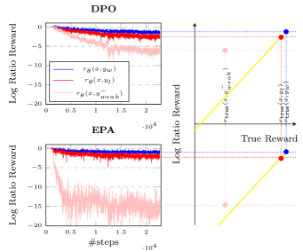
Figure 1: Samples are off from the slope-1 linearity (yellow lines) after training with DPO. Given an extremely undesirable $y_{weak}^{-}$ (i.e., it has very small $r_{\text{true}}$), its $r_{\theta}$ has to be as sufficiently small as $r_{\text{true}}$ to attain the linearity.

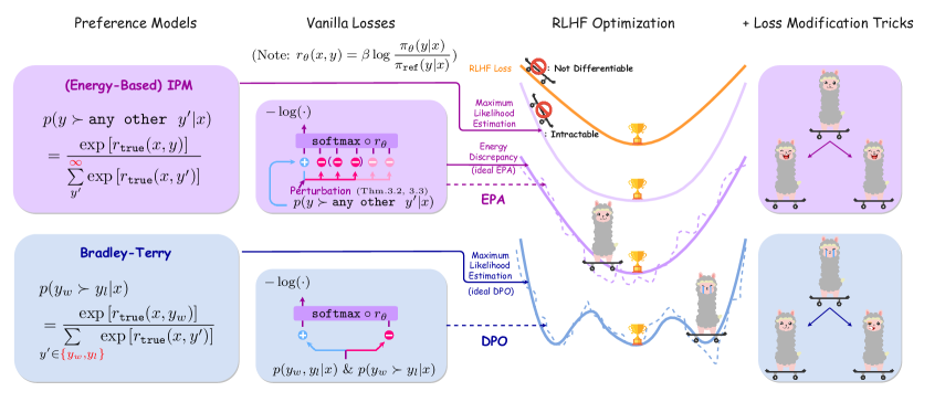
Figure 2: An illustration of the contributions of the paper. Our core argument is that an Energy-Based model (EBM) is a better alternative to the Bradley-Terry model (BTM) due to its guaranteed unique existence of maximum likelihood estimator (MLE) (which is identical to the minimizer of the RLHF loss). The advantage of our EBM comes from its intrinsic consideration of the infinity in the size of the space of $y|x$, whereas BTM ignores issues caused by the pair sampling distribution ($p(y_{w},y_{l}|x)$) in such infinite space. Hence we name our EBM the Infinite Preference Model. Although approximating the MLE with our proposed EPA loss introduces inevitable error in practice, we find that it is still empirically better performing than its counterpart – DPO, with or without loss modification techniques presented in previous offline alignment literatures.

1 Introduction

Reinforcement Learning with Human Feedback (RLHF) (Christiano et al., 2017) has been widely used to align a large language model (LLM) with human preference. The canonical RLHF objective (Ziegler et al., 2019; Stiennon et al., 2020; Ouyang et al., 2022; Perez et al., 2022) is defined as follows (given $x$):

$$\mathcal{L}_{\text{RLHF}}=$$ (1)

$$-\mathop{\mathbb{E}}_{\pi_{\theta}(y|x)}[r_{\text{true}}(x,y)]+\beta\text{KL}[\pi_{\theta}(y|x)||\pi_{\text{ref}}(y|x)]$$

where $\pi_{\theta}(y|x)$ is the target LLM (i.e., the policy) to tune, $\pi_{\text{ref}}(y|x)$ a frozen LLM initialized identically as the target LLM and $r_{\text{true}}(x,y)$ a reward to maximize.

The $\mathcal{L}_{\text{RLHF}}$ as defined above is not differentiable w.r.t $\theta$ (Ziegler et al., 2019; Rafailov et al., 2023), hence not SGD-friendly. Luckily, it has been shown that the unique minimizer of $\mathcal{L}_{\text{RLHF}}$ can be analytically expressed (Korbak et al., 2022a). Then, Rafailov et al. (2023) further reformulate the analytical minimizer as the unique solution to the following set of equations:

$$[left=\empheqlbrace]\text{\small$r_{\theta}(x,y)$} =\beta\log\frac{\pi_{\theta}(y|x)}{\pi_{\text{ref}}(y|x)}$$ (2)

$$r_{\theta}(x,y) =r_{\text{true}}(x,y)+C(x)$$ (3)

Eq.(2) defines $r_{\theta}$ as the log ratio reward and Eq.(3) states that there holds a slope-1 linearity between the log ratio reward and the true reward. This formulation implies that as long as we can find a differentiable objective function $\mathcal{L}(r_{\theta})$ to achieve Eq.(3) and $r_{\theta}$ is parameterized by Eq.(2), we can convert the RLHF problem into an offline supervised task. This is the approach of interest in this paper, a drastically different one from classical online RL methods such as PPO.

1.1 Background & Motivation

The poster child example of this offline approach is DPO (Rafailov et al., 2023):

$$\text{\small$\mathcal{L}_{\text{DPO}}^{\text{ideal}}(r_{\theta})=$}$$ (4)

$$\text{\small$-\mathop{\mathbb{E}}_{p(y_{w},y_{l}|x)}\mathop{\mathbb{E}}_{p(y_{w}\succ y_{l}|x)}[\log\sigma(r_{\theta}(x,y_{w})-r_{\theta}(x,y_{l}))]$}$$

where $y_{w}$ and $y_{l}$ are two responses and $y_{w}\succ y_{l}$ means $y_{w}$ is prefered to $y_{l}$ given the prompt $x$. The ideal DPO loss is essentially the maximum likelihood estimation loss of the Bradley-Terry model (BTM) who posits a sigmoidal relationship between $p(y_{w}\succ y_{l}|x)$ and $r_{\text{true}}(x,y_{w})-r_{\text{true}}(x,y_{l})$. If the maximum likelihood estimator (MLE) uniquely exists, Rafailov et al. (2023) show that the MLE will make the slope-1 linearity hold.

However, as alluded to by our framing, we argue that it is false to conclude that the slope-1 linearity (i.e., the minimizer of the RLHF loss) is guaranteed to be reached with DPO. The reason is that the unique existence of BTM’s MLE (i.e., the minimizer of $\mathcal{L}_{\text{DPO}}$) is not guaranteed without some non-trivial constraints on the structure of $p(y_{w},y_{l}|x)$, a well-known issue of BTM given an infinite candidate space (i.e., that of $y|x$) in the literature on learning to rank (Ford, 1957; Simons & Yao, 1999; Han et al., 2020; Hendrickx et al., 2020; Bong & Rinaldo, 2022; Wu et al., 2022). It is also related to the theoretical issues around dataset coverage in the RL literature (Kakade & Langford, 2002; Munos & Szepesvári, 2008; Zhan et al., 2022). Moreover, Tang et al. (2024) have shown that when offline data are from $\pi_{\text{ref}}$ (a usual practice), any pair-wise loss will cease to correlate with $\mathcal{L}_{\text{RLHF}}$ when $\pi_{\theta}$ deviates enough from $\pi{{}_{\text{ref}}}$ due to reward maximization. This is the theoretical side of our motivation.

A preliminary experiment also evidently shows that DPO does not achieve the slope-1 linearity. Assuming it does, we should expect $r_{\theta}(x,y_{w})>r_{\theta}(x,y_{l})\gg r_{\theta}(x,y_{weak}^{-})$ because the true rewards are certainly so if weak negatives ($y_{weak}^{-}$) are mismatched inputs and outputs as they are almost impossible to be preferred. However, as shown in Figure 1, we find that their log ratio rewards are not substantially lower than the strong negatives ($y_{l}$) when training with DPO. This empirical phenomenon motivates us to find a method that utilizes the free signal offered by $y_{weak}^{-}$.

1.2 Contributions

Our proposal brings the theoretical and the empirical sides together. As shown in Figure 2, we argue that an Energy-Based model (EBM) called the Infinite Preference Model (IPM) is superior to BTM in preference modeling for offline alignment based on the following contributions:

• theoretically showing IPM has guaranteed unique existence of its MLE, equivalent to the minimizer of the RLHF loss;

• the proposal of EPA, an offline contrastive loss to estimate the MLE of IPM by explicitly using weak negatives in addition to strong negatives;

• a new state of the art of offline alignment on open benchmarks when given the same settings of training data and usage of tricks to tweak the losses.

2 Related work

2.1 DPO and its recent improvements

The first approach to avoid DPO’s theoretical issue is to use non-BTMs to model data distributions. Rafailov et al. (2023) suggest the DPO’s counterpart for the Plackett-Luce Model (we refer to it as DPO-PL), which is a generalized version of BTM for K-wise comparison. IPO (Azar et al., 2023) uses a different pair-wise preference model than BTM. The loss derived from that model can be interpreted as: the difference of log ratio rewards of the $y_{w}$ and $y_{l}$ regresses to a constant. However, Tang et al. (2024) show that IPO is still incapable of optimizing $\mathcal{L}_{\text{RLHF}}$, similar to DPO. Ethayarajh et al. (2024) (KTO) point out some limitations of modeling human preference with a pair-wise model. Instead, they independently model a data distribution for desirable samples and another one for undesirable samples. However, such data distributions do not reflect how most benchmark datasets are sampled. This could be the reason why some empirically driven studies find that KTO underperforms DPO on these benchmarks (Meng et al., 2024; Zhou et al., 2024).

The second approach is to tweak the DPO loss. Some loss-tweaking tricks can be effective on their own. For example, cDPO (Mitchell, 2023) uses label smoothing to alleviate DPO’s overfitting problem. Park et al. (2024) (R-DPO) introduce a length penalty on the log ratio reward to make DPO less prone to the verbosity bias. Amini et al. (2024) (ODPO) add a dynamic margin between $y_{w}$ and $y_{l}$ based on the intuition that some pairs have stronger or weaker desirability gaps than others. The most effective one discovered so far is on-policy weighting (WPO) (Zhou et al., 2024). Its idea is to approximate the on-policy training scenario by assigning larger weights to the loss of samples closer the current policy at each step and smaller weights to that of less closer ones. Other tricks come in combinations. For example, CPO (Xu et al., 2024) removes the reference model in the log ratio reward and add an SFT loss at the same time. ORPO (Hong et al., 2024) is an improvement over CPO by adding yet another set of tricks: normalizing the policy to the token level (length normalization) and then contrasting the policy distribution with one minus itself. To separate the wheat from the chaff, Meng et al. (2024) find the most simple and effective recipe: removing the reference model, adding a margin and applying length normalization, which gives rise to SimPO.

There is also a hybrid approach of the above two: non-BTMs + tricks. For example, PRO (Song et al., 2024) is on top of DPO-PL, and BCO (Jung et al., 2024) on top of KTO.

The problem with applying tricks is that there is usually a lack of theoretical justification on how they are related to the minimizer of the RLHF loss.

2.2 Fitting discrete EBMs

To provide a theoretical background for our proposal, we give a concise review of the most related work on fitting discrete EBMs.

Energy-based models (EBM) (LeCun et al., 2006) are generative models that posit a Boltzmann distribution of data, i.e., $p(x)\propto\exp{(-E(x))}$ where $E(x)$ (called the energy function) is a real-valued function to learn. An EBM is called discrete when the data point $x$ is defined on a discrete space. To fit $p(x)$ with maximum likelihood estimation requires the computation of the normalizer $\Sigma_{x^{{}^{\prime}}}^{\infty}\exp{(-E(x^{{}^{\prime}}))}$ (called the partition function), which is intractable. Therefore, EBMs are usually learned with a tractable approximation.

The classical approach is to approximate the gradient of maximum likelihood estimation by online sampling from parameterized $p_{\theta}(x)$ with MCMC (Song & Kingma, 2021). Although they are ideally effective, it is usually difficult or expensive to do such sampling, which harms practical results. Therefore, there are also many MCMC-free methods (Meng et al., 2022; Hyvärinen, 2007; Dai et al., 2020; Lazaro-Gredilla et al., 2021; Eikema et al., 2022). Recently, Schröder et al. (2023) have introduced the notion of energy discrepancy, whose unique global minimizer is identical to the MLE of the EMB in question. Hence, to find the MLE, one can simply minimize the energy discrepancy, which is feasible with SGD on offline data. For its simplicity, we derive EPA based on their theoretical framework.

2.3 EBMs for RLHF

EBMs are not rare in the RLHF research. One of the research directions is to formulate RLHF as a Distribution Matching problem: minimization of the KL divergence between a target EBM that reflects human preference and the policy. The typical example for this approach is Distributional Policy Gradients (DPG) (Parshakova et al., 2019; Khalifa et al., 2021). However, we would like to point out that our EBM is different and used for a different purpose. The EBM in DPG is a non-parametric one predefined as the learning signal. Our EBM is a parametric one to fit the distribution of data. The only connection between the two EBMs is that they are used to find the same optimal policy (Korbak et al., 2022a).

Deng et al. (2020) uses an EBM for language modeling. Their work essentially solves the self-play-like RLHF problem (Chen et al., 2024b). They use the algorithm of Noise Contrastive Estimation (NCE) of fit their EBM. Although their EBM is also parametric, it fits the optimal policy distribution. Our EBM instead fits the preference distribution.

Chen et al. (2024a) proposes two methods – infoNCA and NCA, based on the same EBM as that of Deng et al. (2020). The NCA loss follows the same derivation of the loss proposed by Deng et al. (2020) except that they parameterize their energy function differently. The infoNCA loss exhibits similarity to our loss. However, we will show that infoNCA is just a worse-performing ablation version of EPA.

3 IPM: Our EBM for Preference Modelling

In the first subsection, we show that an energy-based model (EBM) is guaranteed to have a unique MLE which is equivalent to the minimizer of the RLHF objective. In the second subsection, based on a framework by Schröder et al. (2023), we describe a general strategy to approximate the MLE using offline data. Using it will provide the theoretical account for our proposal in section 4.

3.1 Theoretical guarantee

Given any $x$, it is obvious that the space of $y|x$ is infinitely large because $y$ can be any token sequence of unlimited length no matter how likely or unlikely it is a response to $x$. This infinity is problematic for BTM. For example, if there is a single $y$ that is never sampled, it is easy to refute the unique existence of BTM’s MLE (see Proposition B.5). However, EBM can naturally take the infinity into account to avoid the issue. Specifically, we model a one-to-infinite preference (v.s. BTM and the more general Plakett-Luce model only model a one-to-finite-number preference) as follows:

$$p(y|x)\coloneqq p(\forall y^{\prime}\neq y:\ y\succ y^{\prime}|x)$$ (5)

Namely, $p(y|x)$ is the probability that candidate $y$ is preferred over all other candidates. Under mild assumptions (Assumptions B.1 and B.2) that make an EBM applicable, we define the Infinite Preference Model (IPM) to be the one that posits that $p(y|x)$ is a Boltzmann distribution induced by the corresponding true reward (i.e., using $-r_{\text{true}}(x,y)$ as the energy function):

$$p(y|x)=\frac{\exp[r_{\text{true}}(x,y)]}{\Sigma_{y^{{}^{\prime}}}^{\infty}\exp[r_{\text{true}}(x,y^{{}^{\prime}})]}$$ (6)

IPM is a better alternative to BTM because of the following theorem (see Appendix B for proof).

Theorem 3.1.

when we parameterize the IPM as follows, the unique existence of the IPM’s MLE is guaranteed and it will be reached if and only if the slope-1 linearity (i.e., Eq.(3)) holds between the log ratio reward and the true reward.

$$q_{\theta}(y|x)=\frac{\exp[r_{\theta}(x,y)]}{\Sigma_{y^{{}^{\prime}}}^{\infty}\exp[r_{\theta}(x,y^{{}^{\prime}})]}$$ (7)

where $r_{\theta}$ is defined as in Eq.(2).

Therefore, as long as we can find the MLE of the IPM parameterized as so, we are guaranteed to reach the minimizer of $\mathcal{L}_{\text{RLHF}}$ since it is the unique solution to Eq.(2) and Eq.(3).

On a side note, the IPM has been previously introduced by other studies on RLHF for a different purpose: to theoretically equate the maximization of $-\mathcal{L}_{\text{RLHF}}$ to the variational inference of the optimal policy with $\pi_{\text{ref}}$ as the prior (Korbak et al., 2022b; Yang et al., 2024). However, to the best of our knowledge, we are the first one to introduce IPM not just as a theoretical toy, but as a tool (when parameterized by the log ratio reward) to do proper RL-free RLHF.

3.2 Offline approximation of MLE

Despite the powerfulness of IPM, finding its MLE is a non-trivial task. Directly finding it with the minimization of the negative log likelihood $-\log q_{\theta}(y|x)$ is intractable because of the infinity in the denominator.

There are good tractable approximations but usually with complex online training algorithms. For simplicity and scalability purposes, we choose to follow Schröder et al. (2023), who provide a general strategy that finds the optimal EBM by simple SGD with offline training data. The strategy is based on two theorems formally adapted for our purpose as follows.

Theorem 3.2.

For any random variable $Z$ with the conditional variance $\text{Var}[Y|Z]$ being positive, the global unique minimizer $r^{*}(x,y)$ of the functional Energy Discrepancy (ED) defined as follows is the optimal IPM (i.e., $p(y|x)\propto\exp{[r^{*}(x,y)]}$).

$$\text{ED}_{x,p(y|x),p(z|y)}[r]\coloneqq$$ (8)

$$\mathop{\mathbb{E}}_{p(y|x)}\mathop{\mathbb{E}}_{p(z|y)}[\log\Sigma_{y^{\prime}}{p(z|y^{\prime})\exp{[r(x,y^{\prime})-r(x,y)]}}]$$

Theorem 3.3.

For any random variable $Z$ whose backward and forward transition probabilities from $Y$ solve the equation $\Sigma_{y}p(z|y)f(y)=\Sigma_{y}p(y|z)f(y)$ for an arbitrary $f$, the estimation error of the following statistic estimate of $\text{ED}_{x,p(y|x),p(z|y)}[r]$ vanishes almost surely when $N\xrightarrow{}\infty$ and $M\xrightarrow{}\infty$.

$$\mathcal{L}[\theta|x]\coloneqq$$ (9)

$$\frac{1}{N}\Sigma_{i}^{N}\log(1+\Sigma_{j}^{M}{\exp{[r_{\theta}(x,y_{-}^{i,j})-r_{\theta}(x,y^{i})]}})$$

$$-\log(M)$$

where $\{y^{i}\}^{N}$ are samples from $p(y|x)$, $\{y_{-}^{i,j}\}^{M}$ from $p(y|z_{0})$, and $z_{0}$ a single sample from $p(z|y^{i})$.

A one-sentence interpretation of the above theorems is: if we have a particular kind of negative sampling strategy by perturbing observed preferred samples, we will learn the optimal IPM by minimizing a contrastive loss between the negatives and observed positives. Therefore, when the IPM is parameterized by the log ratio reward, we will find the exact minimizer of $\mathcal{L}_{\text{RLHF}}$ with this loss function.

Note that the property of the negative sampling source $Z$ as described in Theorem 3.3 is just a sufficient condition as opposed to a necessary one. This leaves room for empirical discovery of better negative sampling strategies. A rule of thumb as suggested by Schröder et al. (2023) is that $Z$ has to be informative of $Y$ and of high conditional variance at the same time. This provides the intuition of our proposal in section 4.

4 EPA: A Practical Approximation

To introduce our loss, we first write the ideal loss in Eq.(9) in an equivalent form by removing the constant $\log(M)$ and moving a minus sign out of the logarithm:

$$\tilde{\mathcal{L}}[\theta|x]\coloneqq$$ (10)

$$\frac{1}{N}\Sigma_{i}^{N}-\log\frac{\exp[r_{\theta}(x,y^{i})]}{\exp[r_{\theta}(x,y^{i})]+\Sigma_{j}^{M}\exp[r_{\theta}(x,y_{-}^{i,j})]}$$

Now we propose our loss function in this negative log softmax form with a specific negative sampling strategy in mind.

4.1 Narrow definition

For the most classical setup, we assume we only have access to pair-wise preference data. In this setting, our loss for each mini-batch of $B$ samples ($\{(x^{i},y_{w}^{i},y_{l}^{i})\}^{B}$) is defined as follows:

$$\begin{aligned} &\text{\small$\mathcal{L}_{\text{EPA}}=$}\\ &\text{\small$\frac{1}{B}\sum\limits_{i}^{B}-\log\frac{\exp[r_{\theta}(x^{i},y_{w}^{i})]}{\sum\limits_{\mathclap{j\in\{i\}\cup\mathcal{I}_{\text{wk}}}}\big{(}\exp[r_{\theta}(x^{i},y_{w}^{j})]+\exp[r_{\theta}(x^{i},y_{l}^{j})]\big{)}}$}\end{aligned}\hskip-11.99998pt$$ (11)

where $\mathcal{I}_{\text{wk}}$ is a non-empty random subset of $\{1,\ 2,\ \dots,\ i-1,\ i+1,\ \dots,\ B\}$, introducing negative samples that are mismatched responses originally sampled for other prompts. Its size $|\mathcal{I}_{\text{wk}}|=N^{-}_{weak}/2\in(0,B-1]$ is a hyperparameter. Note that our loss without $\mathcal{I}_{\text{wk}}$ reduces to the DPO loss. We justify our choice of positives and negatives in EPA as follows:

1. Why is $y_{w}$ a good approximation of a positive sample from $p(y|x)$? For a $y_{w}$ in the dataset, it may not be the best $y$, but there is only a finite number of potentially possible better ones according to Assumption B.1. Also, since we know it is preferred over $y_{l}$ and infinitely many other arbitrary token sequences, it is a good approximation of a $y$ that is preferred over all other samples up to a small error.

2. Why use both $y_{l}$ and mismatched responses as negatives? As stated at the end of section 3, we want to draw the negatives from a perturbation source that is both informative of the positives and of high variance at the same time. For the informativeness, we consider strong negatives $y_{l}$ because they are semantically close to $y_{w}$. For the high variance, we consider weak negatives such as mismatched responses. We will show the effectiveness of such choice with ablation experiments in section 5.

4.2 General definition

Note that the number of strong negatives in Eq.(11) is limited to 1 because of the given pair-wise data. This is not ideal for the approximation of IPM’s MLE because the number of negatives should be large enough to reduce the approximation error (Theorem 3.3). Therefore, in order not to limit the power of IPM by the classical pair-wise data setup, we generalize our definition of EPA to circumstances where we can have access to more strong negatives (i.e., each $y_{w}$ is accompanied by $\{y_{l_{1}},\ y_{l_{2}},\ \dots\}$ instead of just one $y_{l}$). This is practically feasible because we can always sample less desirable responses from some LLM.

Hence, we define our loss in a more general form as follows:

$$\begin{aligned} &\mathcal{L}_{\text{EPA}}^{\text{general}}=\\ &\text{\tiny$\frac{1}{B}\sum\limits_{i}^{B}-\log\frac{\exp[r_{\theta}(x^{i},y_{w}^{i})]}{\exp[r_{\theta}(x^{i},y_{w}^{i})]+\sum\limits_{\mathclap{k\in\mathcal{I}_{\text{st}}}}\exp[r_{\theta}(x^{i},y_{l_{k}}^{i})]+\sum\limits_{\mathclap{j\in\mathcal{I}_{\text{wk}}}}\exp[r_{\theta}(x^{i},y_{*}^{j})]}$}\end{aligned}\hskip-11.99998pt$$ (12)

where $\mathcal{I}_{\text{st}}$ contains $N^{-}_{strong}$ indices of available strong negatives; $\mathcal{I}_{\text{wk}}$ contains $N^{-}_{weak}$ indices of weak negatives; $y_{*}^{j}$ can be either $y_{w}^{j}$ or some $y_{l_{k}}^{j}$ ($j\neq i$). The justification for the choice of the positives, strong and weak negatives is the same as that of the narrow definition.

4.3 Gradient analysis

Using the chain rule consecutively on the negative log softmax and the log ratio reward, one can easily find the gradient of the EPA loss (the general one) as follows:

$$\hskip-14.22636pt\begin{aligned} \nabla_{\theta}\mathcal{L}_{\text{EPA}}^{\text{general}}&=\\ \text{\footnotesize$-\frac{\beta}{B}\sum\limits_{i}^{B}\Big{(}$}&\text{\footnotesize$\underbrace{\sum\limits_{k\in\mathcal{I}_{\text{st}}}s^{i}_{l_{k}}\big{(}\nabla_{\theta}\log\pi_{\theta}({y^{i}_{w}}|x^{i})-\nabla_{\theta}\log\pi_{\theta}({y^{i}_{l_{k}}}|x^{i})\big{)}}_{\text{strong contrast}}$}\\ +&\text{\footnotesize$\underbrace{\sum\limits_{j\in\mathcal{I}_{\text{wk}}}s^{j}\big{(}\nabla_{\theta}\log\pi_{\theta}({y^{i}_{w}}|x^{i})-\nabla_{\theta}\log\pi_{\theta}({y^{j}_{*}}|x^{i})\big{)}}_{\text{weak contrast}}\Big{)}$}\end{aligned}\hskip-11.99998pt$$ (13)

where $s^{i}_{l_{k}}$ and $s^{j}$ are the softmax-ed values of the strong negative log ratio rewards and the weak negative log ratio rewards, respectively. They control the magnitude of the strong and weak contrast. When there is no weak contrast, the gradient reduces to that of the DPO loss if there is only one strong negative. Therefore, one can interpret the weak contrast as a regularization term added to DPO to prevent $\theta$ from moving to a direction that undesirably increases the likelihood of weak negatives.

5 Experiments

5.1 Experimental setup

5.1.1 Training Data

We consider the dataset of Ultrafeedback (Cui et al., 2024) (denoted as ‘UF-all’) and a widely used pair-wise version of it (Tunstall et al., 2023) (UF-binarized). The two datasets are ideal for our purpose besides their popularity. Firstly, in UF-all, there are 4 responses sampled from multiple sources for each prompt. This will allow training with our general version of EPA which can utilize multiple strong negatives. Secondly, in both UF-all and UF-binarized, the positive sample $y_{w}$ for each $x$ is the best one out of the 4 responses. This is an arguably close approximation to our assumption that positives are sampled from $p(\forall y^{\prime}\neq y:\ y\succ y^{\prime}|x)$.

5.1.2 Evaluation

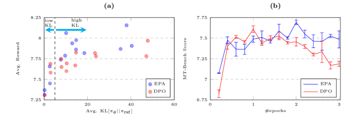
Figure 3: DPO vs. EPA (1:1:2) from the perspective of (a) KL-Reward frontier and (b) training dynamics.

Although Ultrafeedback is intended to reflect human preference, it is labeled by GPT-4 in reality. Consequently, we consider MT-Bench (Zheng et al., 2024) which also uses GPT-4 to score a response on a scale of 1-10. The metric is the average score for 80 single-turn conversations and 80 multi-turn conversations. We also consider Alpaca-Eval 2.0 (Dubois et al., 2024) because of its high correlation with human preference, the ultimate concern for RLHF. Its metrics are win-rates (with or without length control) against GPT-4-turbo across 805 test samples with the judge being GPT-4-turbo itself. We report them in the format of “length controlled win-rate / win-rate” in the experiment results. For evaluation on Alpaca Eval 2.0, we use the default decoding parameters in the Huggingface implementation. For MT-Bench, we use the ones specifically required by the benchmark.

5.1.3 Baselines & loss modification tricks

Training Data	Method	AE 2.0 (%)	MT-Bench
	SFT	8.16 / 5.47	6.44
1-4 UF-binarized	+DPO	17.43 / 15.24	7.55
	+IPO	12.97 / 10.13	7.31
	+KTO	12.62 / 11.29	7.21
	+NCA	14.64 / 11.27	7.39
2-4	+EPA	19.20 / 19.26	7.71
UF-all	+DPO-PL	15.95 / 14.68	7.57
	+NCA	15.08 / 11.85	7.28
	+infoNCA	17.30 / 16.25	7.50
2-4	+EPA	22.03 / 21.44	7.58

Table 1: EPA beats all other baselines either for pair-wise data or for data with $>2$ responses for each prompt.

For fair comparison, we only consider methods from the approach that explicitly aims to minimize $\mathcal{L}_{\text{RLHF}}$ with specific probabilistic models about data distributions. Therefore, we consider DPO, IPO, KTO and NCA for the classical pair-wise data setting. We consider DPO-PL, NCA, and infoNCA for the general setting where there are multiple responses for each prompt in the dataset.

Loss modification tricks are not considered as baselines because they are orthogonal to our proposal. Comparing BTM+tricks to EBM would be comparing apples to oranges. Instead, we consider applying the tricks to both EPA (the narrow one for fair comparison) and DPO to further verify our core argument about EBM’s superiority over BTM. The tricks in consideration are those used in SimPO, R-DPO, CPO and WPO (Details in Table LABEL:tab:listoftricks in the Appendix LABEL:apdx:b).

5.1.4 Implementation

We use mistral-7b-sft-beta as the reference model and for the initialization of policy in our paper. We train all models in this paper for 3 epochs with LoRA ($r=16$, $\alpha=16$, dropout $=0.05$). Whenever comparing among different methods, we pick the one out of the three checkpoints with the best MT-Bench score for each method. For fair comparison of baseline models, we fix $\beta$ to 0.01. It is more of a control variable than a hyperparameter because it is a given component of the RLHF objective which all baselines are aimed to optimize. We only vary $\beta$ for them when probing their KL-Reward frontiers. For comparison of loss modification tricks, since the RLHF objective is not necessarily the purpose, we use the best $\beta$ and other hyperparameters specific to each method as reported in previous work (e.g., the tricks used in SimPO are only competitive when $\beta=2.0$ for the Mistral model). Learning rate is grid-searched for each method among $\{1e-5,5e-6,1e-6\}$.

5.2 Results and analysis

5.2.1 EPA performs better than baselines

As shown in Table 5.1.3, we can see EPA consistently achieves the highest scores and hence a new state of the art. Note that other baselines generally perform even less well than DPO. This makes BTM the strongest baseline for EBM.

5.2.2 EPA $>=$ DPO for the optimization of $\mathcal{L}_{\text{RLHF}}$

To compare our EBM with its most competitive baseline BTM in detail, we come back to the starting point – optimizing $\mathcal{L}_{\text{RLHF}}$. We study from two perspectives of the optimization problem. Both perspectives involve multiple checkpoints beyond the single best one for each method (e.g., Table 5.1.3), offering a more comprehensive comparison.

First, we study how well each method balances the KL term and the reward term in $\mathcal{L}_{\text{RLHF}}$ with varying $\beta\in\{0.01,0.02,0.03,0.04,0.05,0.1,0.5\}$. Both terms are computed on the 80 single-turn prompts in the MT-Bench dataset. We estimate KL with 20 response samples per prompt from each policy distribution. We use the GPT-4 score produced by MT-Bench as an alias for the true reward. As shown in Figure 3.(a), in the high-KL region, EPA generally achieves higher reward than DPO. The two become indistinguishable only in the low-KL region.

Second, to understand how EPA differs from DPO in terms of the dynamics during the optimization process, we test the MT-Bench score of the checkpoint at every 20% of an epoch. As shown in Figure 3.(b), EPA is less prone to overfitting and fits to the reward signal more steadily than DPO. The performance of DPO starts to degenerate rapidly after the first epoch. However, EPA reaches its peak performance at the end of the second epoch and overfits more slowly afterward. This is consistent with our gradient analysis in Section 4 that EPA is more regularized than DPO.

5.2.3 Combining strong and weak negatives is effective

Method	$N^{+}$:$N^{-}_{strong}$:$N^{-}_{weak}$	AE 2.0 (%)	MT-Bench
Ablation	1:1:0 (DPO)	17.43 / 15.24	7.55
	1:0:2	9.37 / 6.74	6.57
1-4 EPA	1:1:1	21.14 / 20.55	7.29
	1:1:2	19.20 / 19.26	7.71
	1:1:6	16.63 / 15.78	7.57
Ablation	1:3:0 (infoNCA)	17.30 / 16.25	7.50
1-4 EPA	1:3:2	22.03 / 21.44	7.58
	1:3:4	21.31 / 20.13	7.58
	1:3:6	24.01 / 23.44	7.35
	1:3:8	24.54 / 23.75	7.19
	1:3:10	23.58 / 22.78	7.43

Table 2: Ablation and variants of EPA with varying number of strong negatives ($N^{-}_{strong}$) and varying number of weak negatives ($N^{-}_{weak}$) in addition to the 1 positive ($N^{+}=1$) in the denominator of $\mathcal{L}^{\text{general}}_{\text{EPA}}$.

We also run ablation and variants of EPA for different numbers of strong and weak negatives. As shown in Table 5.2.3, we can see that although weak negatives are not competitive on its own, their presence together with strong negatives can greatly improve the alignment performance over alternatives with only strong negatives. Moreover, we also find that weak negatives can even improve DPO, but DPO is still worse than EPA in that scenario (Table LABEL:tab:dpo_neg in Appendix LABEL:apdx:b).

5.2.4 EBM+tricks $>=$ BTM+tricks

Pref	Loss	AE 2.0 (%)	MT-
Model	Modification		Bench
BTM	N/A (DPO)	17.43 / 15.24	7.55
2-4	$-ref+\mathcal{L}_{sft}$ (CPO)	13.63 / 10.34	7.11
2-4	$+{len}_{p}$ (R-DPO)	19.10 / 16.71	7.70
2-4	$-ref+{len}_{n}+m_{c}$ (SimPO)	20.57 / 20.19	7.61
2-4	$+{w}_{op}$ (WPO)	21.90 / 21.04	7.56
2-4	$+{m}_{c}$	22.33 / 20.61	7.67
EBM	N/A (EPA)	19.20 / 19.26	7.71
2-4	$+{w}_{op}$	22.80 / 22.26	7.61
2-4	$+{m}_{c}$	23.00 / 22.47	7.68

Table 3: BTM vs. EBM with empirically effective loss modification tricks.

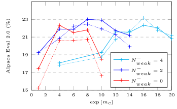
Figure 4: Performance of modified DPO ($N^{-}_{weak}=0$) and modified EPA ($N^{-}_{weak}>0$) with a margin $m_{c}$ added to $r_{\theta}(y_{l}|x)$. Solid lines represent the length-controlled win-rates, and dotted lines represent the raw win-rates.

Since most loss modification tricks presented in the recent offline alignment literature are originally intended for BTM/DPO and do not necessarily make sense to EBM/EPA, we only consider two of them when applying to EPA. The first one is a constant margin $m_{c}$ added to the logit of $y_{l}$. The trick can be viewed as a loose numerical approximation to the general EPA where there are multiple $y_{l_{k}}$. For example, if $m_{c}=1.4$, we have $\exp{[r_{\theta}(x,y_{l})+m_{c}]}=\exp{[m_{c}]}\times\exp{[r_{\theta}(x,y_{l})]}\approx 4\times\exp{[r_{\theta}(x,y_{l})]}$. The second one is the on-policy weight proposed by Zhou et al. (2024). It can be viewed as a curriculum learning technique which prioritizes samples that closely relate to the current policy distribution at each step.

As shown in Table 5.2.4, we find that both $+w_{op}$ and $+{m}_{c}$ produce similar performance boost on EPA to DPO. Although the marginal boost on EPA is generally smaller than DPO, EPA with tricks is still better than DPO with tricks. However, the fact these tricks can still work on EPA also implies that there is still room for improvement. This may come from EPA not necessarily being the best algorithm to approximate our EBM’s MLE.

We also study in detail how the value of ${m}_{c}$ influences DPO and EPA. As shown in Figure 4, we observe that a combination of higher ${m}_{c}$ and higher $N^{-}_{weak}$ tends to produce higher performance. A possible explanation for this is that as ${m}_{c}$ scales up the logit of the strong negative $y_{l}$ to loosely approximate the existence of multiple strong negatives, we get closer to the performance of the general EPA.

6 Conclusion

In this paper, we show both BTM and our EBM have the property that their MLE, if uniquely exists, is equivalent to the minimizer of the RLHF loss. However, the unique existence of EBM’s MLE is guaranteed whereas that of BTM’s MLE is not. This theoretical advantage implies that as long as the EBM’s MLE is accurately found, we are bound to minimize the RLHF loss. But, the same claim does not hold for BTM. Although EPA is just an empirical attempt to approximate our EBM’s MLE, it is already sufficient to outperform its counterpart – DPO on open benchmarks, with or without loss modification tricks presented in previous work.

However, EPA is far from perfect. For example, relatively poorer computation and memory efficiency is a major handicap of EPA. Foreseeable future work includes finding better ways to perturb data or adopting more efficient methods to approximate the MLE. Loss modification tricks particularly tailored for EPA also remain to be explored.

Appendix A Proof of the equivalence between slope-1 linearity and minimizer of the RLHF loss

We do not claim any originality for the proofs given in this section because they are largely just paraphrased versions of the work by Korbak et al. (2022a); Rafailov et al. (2023) and others. We include them just for reference and completeness of the mathematical foundation shared by both DPO and EPA.

Lemma A.1.

The minimizer of the RLHF objective uniquely exists.

Proof.

We show the minimizer $\pi_{r}$ can be analytically expressed by $\frac{1}{Z(x)}\pi_{\text{ref}}(y|x)\exp{\frac{1}{\beta}r(x,y)}$ where $Z(x)=\Sigma_{y}^{\infty}\pi_{\text{ref}}(y|x)\exp{\frac{1}{\beta}r(x,y)}$ (i.e., a normalizer to make $\pi_{r}$ a probabilistic distribution).

From the property of Gibb’s inequality, we know:

$$\begin{aligned} &\text{\small$\pi_{r}=\frac{1}{Z(x)}\pi_{\text{ref}}(y|x)\exp{[\frac{1}{\beta}r(x,y)]}$}\\ &\text{\small$\Leftrightarrow$}\\ &\text{\small$\pi_{r}=\operatorname*{arg\,min}_{\pi_{\theta}}\beta\text{KL}[\pi_{\theta}(y|x)||\frac{1}{Z(x)}\pi_{\text{ref}}(y|x)\exp{\frac{1}{\beta}r(x,y)}]$}\end{aligned}\hskip-11.99998pt$$

We will complete the proof by showing the $\beta$KL-Divergence on the RHS of the above equation is the RLHF objective itself plus a constant w.r.t $\theta$:

$$\begin{aligned} &\beta\text{KL}[\pi_{\theta}(y|x)||\frac{1}{Z(x)}\pi_{\text{ref}}(y|x)\exp{\frac{1}{\beta}r(x,y)}]\\ &=\beta\mathop{\mathbb{E}}_{\pi_{\theta}(y|x)}[\log\frac{\pi_{\theta}(y|x)}{\frac{1}{Z(x)}\pi_{\text{ref}}(y|x)\exp{\frac{1}{\beta}r(x,y)}}]\\ &=\beta\mathop{\mathbb{E}}_{\pi_{\theta}(y|x)}[\log\frac{Z(x)}{\exp[\frac{1}{\beta}r(x,y)]}+\log\frac{\pi_{\theta}(y|x)}{\pi_{\text{ref}}(y|x)}]\\ &=\beta\mathop{\mathbb{E}}_{\pi_{\theta}(y|x)}[\log Z(x)-\frac{1}{\beta}r(x,y)+\log\frac{\pi_{\theta}(y|x)}{\pi_{\text{ref}}(y|x)}]\\ &=-\mathop{\mathbb{E}}_{\pi_{\theta}(y|x)}[r(x,y)]+\beta\text{KL}[\pi_{\theta}(y|x)||\pi_{\text{ref}}(y|x)]\\ &\ \ \ \ \ +\beta\log Z(x)\\ &=\mathcal{L}_{RLHF}(\theta)+\beta\log Z(x)\\ \end{aligned}\hskip-11.99998pt$$

∎

Definition A.2.

We say a slope-1 linearity holds when: r_θ(x, y) = r(x, y) + C(x) where $r_{\theta}(x,y)=\beta\log\frac{\pi_{\theta}(y|x)}{\pi_{\text{ref}}(y|x)}$.

Theorem A.3 (Theorem of necessity).

If $\pi_{\theta}=\pi_{r}$, then slope-1 linearity holds.

Proof.

If $\pi_{\theta}=\pi_{r}$, then according to Lemma A.1, we have: π_θ = 1Z(x)π_ref(y—x)exp1βr(x,y) Take the logarithm of both sides of this equation, we have: logπ_θ = logπ_ref+1βr(x,y) - logZ(x) After moving the two log terms to the same side, we get slope-1 linearity: βlogπθπref = r(x,y) - βlogZ(x) ∎

Theorem A.4 (Theorem of sufficiency).

If slope-1 linearity holds, then $\pi_{\theta}=\pi_{r}$.

Proof.

From the Theorem of necessity, we know: βlogπrπref = r(x,y) - βlogZ(x) Substracting the slope-1 linearity from this equation, we get: βlogπrπref -βlogπθπref = - βlogZ(x) - C(x) Eliminating the non-zero $\beta$ from both sides and taking the exponential, we have: πrπθ = f(x) where $f(x)=\frac{1}{Z(x)\exp[\frac{1}{\beta}C(x)]}$. Moving $\pi_{\theta}$ to the RHS, we get: π_r = π_θf(x) Taking $\Sigma_{y}^{\infty}$ for both sides, we can sum up both distributions $\pi_{r}$ and $\pi_{\theta}$ to one: 1=f(x) Therefore, π_r = π_θf(x) = π_θ ∎

Note that from the above proof, we can easily get the following corollary because $f(x)=1\Leftrightarrow C(x)=-\beta\log Z(x)$.

Corollary A.5.

when a $r_{\theta}$ satisfies slope-1 linearity, it is unique.

Appendix B Theoretical Aspect of the Infinite Preference Model

We will first give our proof of the guaranteed unique existence of our IPM’s MLE. Then, we will discuss how BTM is flawed for an infinite space of $y|x$.

B.1 On IPM’s MLE

We make the following mild assumptions about the structure of human preference:

Assumption B.1.

$\mathcal{D}_{\cdot|x}=\{y|p(y|x)>0\}$ is a finite set.

Assumption B.2.

$r(x,y)\xrightarrow{}-\infty$ for any $y\notin\mathcal{D}_{\cdot|x}$ and $r(x,y)<+\infty$ for any $y\in\mathcal{D}_{\cdot|x}$.

Note that the above two assumptions are just one of many sufficient assumptions that make the partition function exist as a finite real number. Also note that the finity of $\mathcal{D}_{\cdot|x}$ and the infinity of the space of $y|x$ are two different things that can certainly co-exist. Namely, $\mathcal{D}_{\cdot|x}$ is a subset of the space of $y|x$. The number of $y$ outside of $\mathcal{D}_{\cdot|x}$ is still infinitely large. The two assumptions in plain words are simply that we assume humans will only possibly prefer a finite set of responses. Note that this does not mean that the finite set $\mathcal{D}_{\cdot|x}$ cannot be very large.

Definition B.3.

The maximum likelihood estimation objective of IPM is the negative log-likelihood of preference data computed as follows: -Σ_y^∞ p(y—x)logq_θ(y—x) where $p(y|x)=\frac{\exp[r(x,y)]}{\Sigma_{y^{{}^{\prime}}}^{\infty}\exp[r(x,y^{{}^{\prime}})]}$ and $q_{\theta}(y|x)=\frac{\exp[r_{\theta}(x,y)]}{\Sigma_{y^{{}^{\prime}}}^{\infty}\exp[r_{\theta}(x,y^{{}^{\prime}})]}$.

Given the uniqueness in Corollary A.5, we can argue the following:

Theorem B.4 (Theorem 3.1 in the main content of the paper).

The $r_{\theta}$ that satisfies the slope-1 linearity is the unique minimizer of the IPM’s maximum likelihood estimation objective.

Proof.

Again, from the property of Gibb’s inequality, we know:

$$q_{\theta}(y|x)=p(y|x)$$

$$\Leftrightarrow$$

$$q_{\theta}(y|x)=\operatorname*{arg\,min}_{q}\text{KL}[p(y|x)||q(y|x)]$$

For the equation on the right, since $p(y|x)$ is a constant w.r.t $\theta$, we can find $q_{\theta}$ is the minimizer of IPM’s objective:

$$q_{\theta}(y|x) =\operatorname*{arg\,min}_{q}\text{KL}[p(y|x)||q(y|x)]$$

$$=\operatorname*{arg\,min}_{q}\text{H}[p(y|x)]-\Sigma_{y}^{\infty}p(y|x)\log q(y|x)$$

$$=\operatorname*{arg\,min}_{q}-\Sigma_{y}^{\infty}p(y|x)\log q(y|x)$$

We then show that $q_{\theta}(y|x)=p(y|x)$ is equivalent to slope-1 linearity to complete the proof by taking the logarithm of both sides:

$$r_{\theta}(x,y)-C_{1}(x)=r(x,y)-C_{2}(x)$$

$$\Leftrightarrow$$

$$r_{\theta}(x,y)=r(x,y)+C(x)$$

where $C_{1}(x)=\log\Sigma_{y^{{}^{\prime}}}^{\infty}\exp[r_{\theta}(x,y^{{}^{\prime}})]$, $C_{2}(x)=\log\Sigma_{y^{{}^{\prime}}}^{\infty}\exp[r(x,y^{{}^{\prime}})]$ and $C(x)=C_{1}(x)-C_{2}(x)$ ∎

Note that similar proof does not apply to BTM. The fundamental reason is that the $C_{1}(x)$ and $C_{2}(x)$ only become constants when there is an infinity in the sum to cancel out all $y$.

B.2 On Bradley-Terry Model’s Flaw

We will show in Proposition B.5 that a very likely choice of $p(y_{w},y_{l}|x)$ will lead to multiple minimizers for the maximum likelihood estimation of BTM. There are also many other choices of $p(y_{w},y_{l}|x)$ are known to cause the existence of multiple minimizers (Ford, 1957; Bong & Rinaldo, 2022), such as when there is no full connectivity of the graph made by pairs from $p(y_{w},y_{l}|x)$, and when all $y$ candidates can only be paired with a single shared winning $\tilde{y}$, etc. Therefore, there is no guarantee for the MLE’s uniqueness without imposing additional constraints on $p(y_{w},y_{l}|x)$ (i.e, how the pairs are sampled for DPO). For the loosest sufficient constraints discovered so far to ensure the uniqueness, one can refer to Bong & Rinaldo (2022). However, to the best of our knowledge, how such constraints can be applied to DPO has never been studied in the offline alignment literature, which is also out of the scope of this paper. Moreover, in the infinite-candidate scenario, a constraint that is both necessary and sufficient for the uniqueness of BTM’s MLE remains unknown to this day. What makes BTM even more theoretically troublesome in the case of RLHF is that there is also an infinity for the space of $x$ as well. Therefore, strictly speaking, there is an infinite number of BTMs used in DPO. And, the $p(y_{w},y_{l}|x)$ for every $x$ should ensure the uniqueness, in order to make DPO really work as expected. Interestingly, although our EPA loss also needs an infinite number of IPMs in the strict sense, Theorem B.4 (3.1) ensures the MLE uniqueness of all the IPMs.

Proposition B.5.

If there exists a $y^{*}$ that will never be sampled (i.e., $p(y^{*},\cdot|x)=0$ and $p(\cdot,y^{*}|x)=0$), then whenever there is a minimizer for Bradley-Terry’s maximum likelihood estimation, it is not unique.

Proof.

Without losing generality, we set $\beta=1$.

Given the log ratio reward parameterization, we have an intrinsic constraint on $r_{\theta}$: ∑_y’^∞π_refexp[r_θ]=∑_y’^∞π_θ=1

If we assume that there is a unique minimizer $r_{\hat{\theta}}$ to BTM’s maximum likelihood estimation, it certainly satisfies the above constraint: ∑_y’^∞π_refexp[r_^θ]=1

We will then show that another reward also follows the constraint (hence a valid log ratio reward) and shares the same expected data likelihood as $r_{\hat{\theta}}$, which contradicts the uniqueness of $r_{\hat{\theta}}$. We define the other reward as: $\tilde{r}_{\hat{\theta}}(x,y)=$ {

References

- Amini et al. (2024) Amini, A., Vieira, T., and Cotterell, R. Direct preference optimization with an offset. arXiv preprint arXiv:2402.10571, 2024.
- Azar et al. (2023) Azar, M. G., Rowland, M., Piot, B., Guo, D., Calandriello, D., Valko, M., and Munos, R. A general theoretical paradigm to understand learning from human preferences. arXiv preprint arXiv:2310.12036, 2023.
- Bong & Rinaldo (2022) Bong, H. and Rinaldo, A. Generalized results for the existence and consistency of the MLE in the bradley-terry-luce model. In Chaudhuri, K., Jegelka, S., Song, L., Szepesvari, C., Niu, G., and Sabato, S. (eds.), Proceedings of the 39th International Conference on Machine Learning, volume 162 of Proceedings of Machine Learning Research, pp. 2160–2177. PMLR, 17–23 Jul 2022. URL https://proceedings.mlr.press/v162/bong22a.html.
- Chen et al. (2024a) Chen, H., He, G., Su, H., and Zhu, J. Noise contrastive alignment of language models with explicit rewards. arXiv preprint arXiv:2402.05369, 2024a.
- Chen et al. (2024b) Chen, Z., Deng, Y., Yuan, H., Ji, K., and Gu, Q. Self-play fine-tuning converts weak language models to strong language models. arXiv preprint arXiv:2401.01335, 2024b.
- Christiano et al. (2017) Christiano, P. F., Leike, J., Brown, T., Martic, M., Legg, S., and Amodei, D. Deep reinforcement learning from human preferences. Advances in neural information processing systems, 30, 2017.
- Cobbe et al. (2021) Cobbe, K., Kosaraju, V., Bavarian, M., Chen, M., Jun, H., Kaiser, L., Plappert, M., Tworek, J., Hilton, J., Nakano, R., Hesse, C., and Schulman, J. Training verifiers to solve math word problems. CoRR, abs/2110.14168, 2021. URL https://arxiv.org/abs/2110.14168.
- Cui et al. (2024) Cui, G., Yuan, L., Ding, N., Yao, G., He, B., Zhu, W., Ni, Y., Xie, G., Xie, R., Lin, Y., et al. Ultrafeedback: Boosting language models with scaled ai feedback. In Forty-first International Conference on Machine Learning, 2024.
- Dai et al. (2020) Dai, H., Singh, R., Dai, B., Sutton, C., and Schuurmans, D. Learning discrete energy-based models via auxiliary-variable local exploration. Advances in Neural Information Processing Systems, 33:10443–10455, 2020.
- Deng et al. (2020) Deng, Y., Bakhtin, A., Ott, M., Szlam, A., and Ranzato, M. Residual energy-based models for text generation. In International Conference on Learning Representations, 2020. URL https://openreview.net/forum?id=B1l4SgHKDH.
- Dubois et al. (2024) Dubois, Y., Galambosi, B., Liang, P., and Hashimoto, T. B. Length-controlled alpacaeval: A simple way to debias automatic evaluators. arXiv preprint arXiv:2404.04475, 2024.
- Eikema et al. (2022) Eikema, B., Kruszewski, G., Dance, C. R., Elsahar, H., and Dymetman, M. An approximate sampler for energy-based models with divergence diagnostics. Transactions on Machine Learning Research, 2022.
- Ethayarajh et al. (2024) Ethayarajh, K., Xu, W., Muennighoff, N., Jurafsky, D., and Kiela, D. Kto: Model alignment as prospect theoretic optimization, 2024.
- Ford (1957) Ford, L. R. Solution of a ranking problem from binary comparisons. The American Mathematical Monthly, 64(8):28–33, 1957. ISSN 00029890, 19300972. URL http://www.jstor.org/stable/2308513.
- Han et al. (2020) Han, R., Ye, R., Tan, C., and Chen, K. Asymptotic theory of sparse Bradley–Terry model. The Annals of Applied Probability, 30(5):2491 – 2515, 2020. doi: 10.1214/20-AAP1564. URL https://doi.org/10.1214/20-AAP1564.
- Hendrickx et al. (2020) Hendrickx, J., Olshevsky, A., and Saligrama, V. Minimax rate for learning from pairwise comparisons in the BTL model. In III, H. D. and Singh, A. (eds.), Proceedings of the 37th International Conference on Machine Learning, volume 119 of Proceedings of Machine Learning Research, pp. 4193–4202. PMLR, 13–18 Jul 2020. URL https://proceedings.mlr.press/v119/hendrickx20a.html.
- Hendrycks et al. (2020) Hendrycks, D., Burns, C., Basart, S., Zou, A., Mazeika, M., Song, D., and Steinhardt, J. Measuring massive multitask language understanding. CoRR, abs/2009.03300, 2020. URL https://arxiv.org/abs/2009.03300.
- Hong et al. (2024) Hong, J., Lee, N., and Thorne, J. Orpo: Monolithic preference optimization without reference model. arXiv preprint arXiv:2403.07691, 2(4):5, 2024.
- Hyvärinen (2007) Hyvärinen, A. Some extensions of score matching. Computational statistics & data analysis, 51(5):2499–2512, 2007.
- Jung et al. (2024) Jung, S., Han, G., Nam, D. W., and On, K.-W. Binary classifier optimization for large language model alignment. arXiv preprint arXiv:2404.04656, 2024.
- Kakade & Langford (2002) Kakade, S. and Langford, J. Approximately optimal approximate reinforcement learning. In Proceedings of the Nineteenth International Conference on Machine Learning, pp. 267–274, 2002.
- Khalifa et al. (2021) Khalifa, M., Elsahar, H., and Dymetman, M. A distributional approach to controlled text generation. In International Conference on Learning Representations, 2021. URL https://openreview.net/forum?id=jWkw45-9AbL.
- Korbak et al. (2022a) Korbak, T., Elsahar, H., Kruszewski, G., and Dymetman, M. On reinforcement learning and distribution matching for fine-tuning language models with no catastrophic forgetting. Advances in Neural Information Processing Systems, 35:16203–16220, 2022a.
- Korbak et al. (2022b) Korbak, T., Perez, E., and Buckley, C. Rl with kl penalties is better viewed as bayesian inference. In Findings of the Association for Computational Linguistics: EMNLP 2022, pp. 1083–1091, 2022b.
- Langley (2000) Langley, P. Crafting papers on machine learning. In Langley, P. (ed.), Proceedings of the 17th International Conference on Machine Learning (ICML 2000), pp. 1207–1216, Stanford, CA, 2000. Morgan Kaufmann.
- Lazaro-Gredilla et al. (2021) Lazaro-Gredilla, M., Dedieu, A., and George, D. Perturb-and-max-product: Sampling and learning in discrete energy-based models. Advances in Neural Information Processing Systems, 34:928–940, 2021.
- LeCun et al. (2006) LeCun, Y., Chopra, S., Hadsell, R., Ranzato, M., and Huang, F. A tutorial on energy-based learning. Predicting structured data, 1(0), 2006.
- Majerek et al. (2005) Majerek, D., Nowak, W., and Zieba, W. Conditional strong law of large number. Int. J. Pure Appl. Math, 20(2):143–156, 2005.
- Meng et al. (2022) Meng, C., Choi, K., Song, J., and Ermon, S. Concrete score matching: Generalized score matching for discrete data. Advances in Neural Information Processing Systems, 35:34532–34545, 2022.
- Meng et al. (2024) Meng, Y., Xia, M., and Chen, D. Simpo: Simple preference optimization with a reference-free reward. arXiv preprint arXiv:2405.14734, 2024.
- Mitchell (2023) Mitchell, E. A note on dpo with noisy preferences & relationship to ipo, 2023. URL https://ericmitchell.ai/cdpo.pdf.
- Munos & Szepesvári (2008) Munos, R. and Szepesvári, C. Finite-time bounds for fitted value iteration. Journal of Machine Learning Research, 9(5), 2008.
- Ouyang et al. (2022) Ouyang, L., Wu, J., Jiang, X., Almeida, D., Wainwright, C., Mishkin, P., Zhang, C., Agarwal, S., Slama, K., Ray, A., et al. Training language models to follow instructions with human feedback. Advances in neural information processing systems, 35:27730–27744, 2022.
- Park et al. (2024) Park, R., Rafailov, R., Ermon, S., and Finn, C. Disentangling length from quality in direct preference optimization. arXiv preprint arXiv:2403.19159, 2024.
- Parshakova et al. (2019) Parshakova, T., Andreoli, J.-M., and Dymetman, M. Distributional reinforcement learning for energy-based sequential models. Optimization Foundations for Reinforcement Learning Workshop at NeurIPS 2019, 2019. URL https://optrl2019.github.io/assets/accepted_papers/34.pdf.
- Perez et al. (2022) Perez, E., Huang, S., Song, F., Cai, T., Ring, R., Aslanides, J., Glaese, A., McAleese, N., and Irving, G. Red teaming language models with language models. In Proceedings of the 2022 Conference on Empirical Methods in Natural Language Processing, pp. 3419–3448, 2022.
- Rafailov et al. (2023) Rafailov, R., Sharma, A., Mitchell, E., Manning, C. D., Ermon, S., and Finn, C. Direct preference optimization: Your language model is secretly a reward model. In Thirty-seventh Conference on Neural Information Processing Systems, 2023. URL https://openreview.net/forum?id=HPuSIXJaa9.
- Schröder et al. (2023) Schröder, T., Ou, Z., Li, Y., and Duncan, A. B. Training discrete EBMs with energy discrepancy. In ICML 2023 Workshop: Sampling and Optimization in Discrete Space, 2023. URL https://openreview.net/forum?id=kFMpJh75Wo.
- Simons & Yao (1999) Simons, G. and Yao, Y.-C. Asymptotics when the number of parameters tends to infinity in the bradley-terry model for paired comparisons. The Annals of Statistics, 27(3):1041–1060, 1999.
- Song et al. (2024) Song, F., Yu, B., Li, M., Yu, H., Huang, F., Li, Y., and Wang, H. Preference ranking optimization for human alignment. In Proceedings of the AAAI Conference on Artificial Intelligence, volume 38, pp. 18990–18998, 2024.
- Song & Kingma (2021) Song, Y. and Kingma, D. P. How to train your energy-based models. arXiv preprint arXiv:2101.03288, 2021.
- Stiennon et al. (2020) Stiennon, N., Ouyang, L., Wu, J., Ziegler, D., Lowe, R., Voss, C., Radford, A., Amodei, D., and Christiano, P. F. Learning to summarize with human feedback. Advances in Neural Information Processing Systems, 33:3008–3021, 2020.
- Tang et al. (2024) Tang, Y., Guo, Z. D., Zheng, Z., Calandriello, D., Munos, R., Rowland, M., Richemond, P. H., Valko, M., Pires, B. Á., and Piot, B. Generalized preference optimization: A unified approach to offline alignment. arXiv preprint arXiv:2402.05749, 2024.
- Tikhonov & Ryabinin (2021) Tikhonov, A. and Ryabinin, M. It’s all in the heads: Using attention heads as a baseline for cross-lingual transfer in commonsense reasoning. CoRR, abs/2106.12066, 2021. URL https://arxiv.org/abs/2106.12066.
- Tunstall et al. (2023) Tunstall, L., Beeching, E., Lambert, N., Rajani, N., Rasul, K., Belkada, Y., Huang, S., von Werra, L., Fourrier, C., Habib, N., et al. Zephyr: Direct distillation of lm alignment. arXiv preprint arXiv:2310.16944, 2023.
- Wu et al. (2022) Wu, W., Junker, B. W., and Niezink, N. Asymptotic comparison of identifying constraints for bradley-terry models. arXiv preprint arXiv:2205.04341, 2022.
- Xu et al. (2024) Xu, H., Sharaf, A., Chen, Y., Tan, W., Shen, L., Van Durme, B., Murray, K., and Kim, Y. J. Contrastive preference optimization: Pushing the boundaries of llm performance in machine translation. arXiv preprint arXiv:2401.08417, 2024.
- Yang et al. (2024) Yang, J. Q., Salamatian, S., Sun, Z., Suresh, A. T., and Beirami, A. Asymptotics of language model alignment, 2024.
- Yuan et al. (2023) Yuan, H., Yuan, Z., Tan, C., Wang, W., Huang, S., and Huang, F. RRHF: Rank responses to align language models with human feedback. In Thirty-seventh Conference on Neural Information Processing Systems, 2023. URL https://openreview.net/forum?id=EdIGMCHk4l.
- Zhan et al. (2022) Zhan, W., Huang, B., Huang, A., Jiang, N., and Lee, J. Offline reinforcement learning with realizability and single-policy concentrability. In Conference on Learning Theory, pp. 2730–2775. PMLR, 2022.
- Zheng et al. (2024) Zheng, L., Chiang, W.-L., Sheng, Y., Zhuang, S., Wu, Z., Zhuang, Y., Lin, Z., Li, Z., Li, D., Xing, E., et al. Judging llm-as-a-judge with mt-bench and chatbot arena. Advances in Neural Information Processing Systems, 36, 2024.
- Zhou et al. (2024) Zhou, W., Agrawal, R., Zhang, S., Indurthi, S. R., Zhao, S., Song, K., Xu, S., and Zhu, C. Wpo: Enhancing rlhf with weighted preference optimization. arXiv preprint arXiv:2406.11827, 2024.
- Ziegler et al. (2019) Ziegler, D. M., Stiennon, N., Wu, J., Brown, T. B., Radford, A., Amodei, D., Christiano, P., and Irving, G. Fine-tuning language models from human preferences. arXiv preprint arXiv:1909.08593, 2019.