Achieving Dispatchability in Data Centers: Carbon and Cost-Aware Sizing of Energy Storage and Local Photovoltaic Generation

Abstract

Data centers are large electricity consumers due to the high consumption needs of servers and their cooling systems. Given the current crypto-currency and artificial intelligence trends, the data center electricity demand is bound to grow significantly. With the electricity sector being responsible for a large share of global greenhouse gas (GHG) emissions, it is important to lower the carbon footprint of data centers to meet GHG emissions targets set by international agreements. Moreover, uncontrolled integration of data centers in power distribution grids contributes to increasing the stochasticity of the power system demand, thus increasing the need for capacity reserves, which leads to economic and environmental inefficiencies in the power grid operation.
This work provides a method to size a PhotoVoltaic (PV) system and an Energy Storage System (ESS) for an existing data center looking to reduce both its carbon footprint and demand stochasticity via dispatching. The proposed scenario-based optimization framework allows to size the ESS and the PV system to minimize the expected operational and capital costs, along with the carbon footprint of the data center complex. The life cycle assessment of the resources, as well as the dynamic carbon emissions of the upstream power distribution grid, are accounted for while computing the day-ahead planning of the data center aggregated demand and PV generation. Case studies in different Swiss cantons and regions of Germany emphasize the need for location-aware sizing processes since the obtained optimal solutions strongly depend on the local electricity carbon footprint, cost and on the local irradiance conditions. Some regions show potential in carbon footprint reduction, while other regions do not.

1 Introduction

Data centers consumed $460\text{\,}\mathrm{TW}\text{\,}\mathrm{h}$ of electricity worldwide in 2022, representing almost 2% of the total electricity demand [eren_cam_electricity_2024]. The International Energy Agency (IEA) expects the data center global yearly demand to range between 650 and $1050\text{\,}\mathrm{TW}\text{\,}\mathrm{h}$ in 2026, potentially representing up to 4.5% of the global electricity demand. In Ireland and Denmark, the data center electricity consumption represents respectively 13% and 8% of the country’s demand and it is expected to grow to 30% and 20% by 2026. With the electricity and heat sector accounting for 14.8 billions of tons of $\text{\,}\mathrm{C}\mathrm{O}_{\mathrm{2}}\mathrm{e}\mathrm{q}$ [iea_electricity_2023] (i.e., approximately 25% of global GreenHouse Gases (GHG) emissions worldwide), reducing the carbon footprint of data centers is important to meet GHG emissions targets set by international agreements (e.g., [noauthor_paris_2015]). Additionally, uncontrolled data centers tend to increase the stochasticity of the power system demand and to contribute to an environmentally and economically suboptimal operation of power grids [bhagwat_effectiveness_2017, elcom_equilibre_2024]. For these reasons, carbon-aware solutions for data center modeling, strategic planning/design and management have been presented in the literature, with more than 2500 publications resulting from an IEEE Xplore advanced search combining the keywords "green" and "data center" [noauthor_green_nodate]. However, in practice, Data Center Operators (DCO) often purchase renewable energy or renewable energy credits to match their annual demand [noauthor_google_2019, noauthor_microsoft_2024]. This approach has been shown to be inefficient and misleading as it cannot guarantee an actual reduction of the carbon footprint of the entity making the purchase [bjorn_renewable_2022, shannon__osaka_buying_2023], thus highlighting the need for precise and granular carbon accounting [noauthor_carbon_2023].

1.1 Background

Strategic planning of data centers has been studied with a general focus on methods to reduce their operational costs. For instance, [guo_integrated_2021] formulates a multi-objective optimization problem to determine the optimal capacity and location of a data center and associated energy storage systems, minimizing the costs and maximizing the Quality of Service (QoS). [yong_scheduling_2024] proposes a day-ahead scheduling of data centers based on the concept of a Virtual Power Plant (VPP), leveraging the flexibility of workloads (i.e., using workload migration and shifting), and the flexibility of back-up power devices (i.e., UPSs). Some works on the planning of data centers consider their direct carbon footprint. For instance, [kong_greenplanning_2016] formulates a framework to select energy resources, balancing energy sources with grid power and storage in terms of cost, direct emissions and service availability. [thompson_optimization_2016] presents a sizing method for battery storage systems in data center microgrids. The method allows for costs and emissions reductions by leveraging batteries to shift the peak period demand to off-peak ones. In [wang_day-ahead_2017], a day-ahead direct emission aware-planning of data centers is formulated, where conventional power units and energy storage systems are jointly optimized with batch workload allocation. In [rahmani_modelling_2020], the sizing of wind and PV generation to minimize the operational cost and emissions of a green data center is addressed.

1.2 Contributions and proposed method

As discussed in Section˜1.1, although some studies have been focusing on carbon-aware strategic planning of data centers, the majority of the available literature focuses on operational cost minimization. The studies that take the carbon emissions into consideration rely on simplistic approaches by focusing on direct emissions [kong_greenplanning_2016, wang_day-ahead_2017], or on qualitative information [rahmani_modelling_2020]. In [dou_carbon-aware_2017, radovanovic_carbon-aware_2021, lin_adapting_2023] the hourly average carbon emissions of the grid are taken into account to reduce the footprint of data centers. [lin_adapting_2023] highlights the need for a day-ahead scheduling of the data center power consumption to effectively reduce the carbon emissions. These studies leverage the intrinsic flexibility of the data center, but do not study the flexibility of co-located Distributed Energy Resources (DER) and, therefore, do not assess the optimal sizing of these DER associated to data centers. Finally, while [acun_carbon_2022] proposes a framework to design carbon-aware data centers with DER, it does not consider economic costs and focuses on 24/7 renewable coverage for the data center, which might not be the optimal system design in terms of total carbon footprint since the $\text{\,}\mathrm{C}\mathrm{O}_{\mathrm{2}}$ content of the data center electricity supply varies over time and is location dependent.
In view of the above, this work addresses the problem of carbon-aware sizing of energy storage and photovoltaic generation for existing data centers targeting day-ahead dispatchability (i.e., to track, in real-time, a power profile computed day-ahead). The sizing method allows for geographically and temporally granular grid carbon emissions awareness, while also enabling custom operational cost considerations. The proposed method relies on scenario-based optimization, and is thus capable of taking into account the non-parametric forecasts of the grid carbon intensity, electricity costs, solar irradiance and data center demand. Local considerations (e.g., demand specificities, electricity pricing schemes, etc.) can be easily included in the framework by using precise local data and custom forecasting methods for the stochastic variables.

2 Method

2.1 Overview

2.1.1 Problem statement

The method addresses the optimal sizing of local energy storage and photovoltaic generation to achieve the dispatchability of a data center. The problem determines the optimal ratings of an Energy Storage System (ESS) and PV generation to minimize the expected value of a multi-objective function consisting in the weighted sum of carbon and financial costs. The configuration that is considered is shown schematically in Fig.˜1.

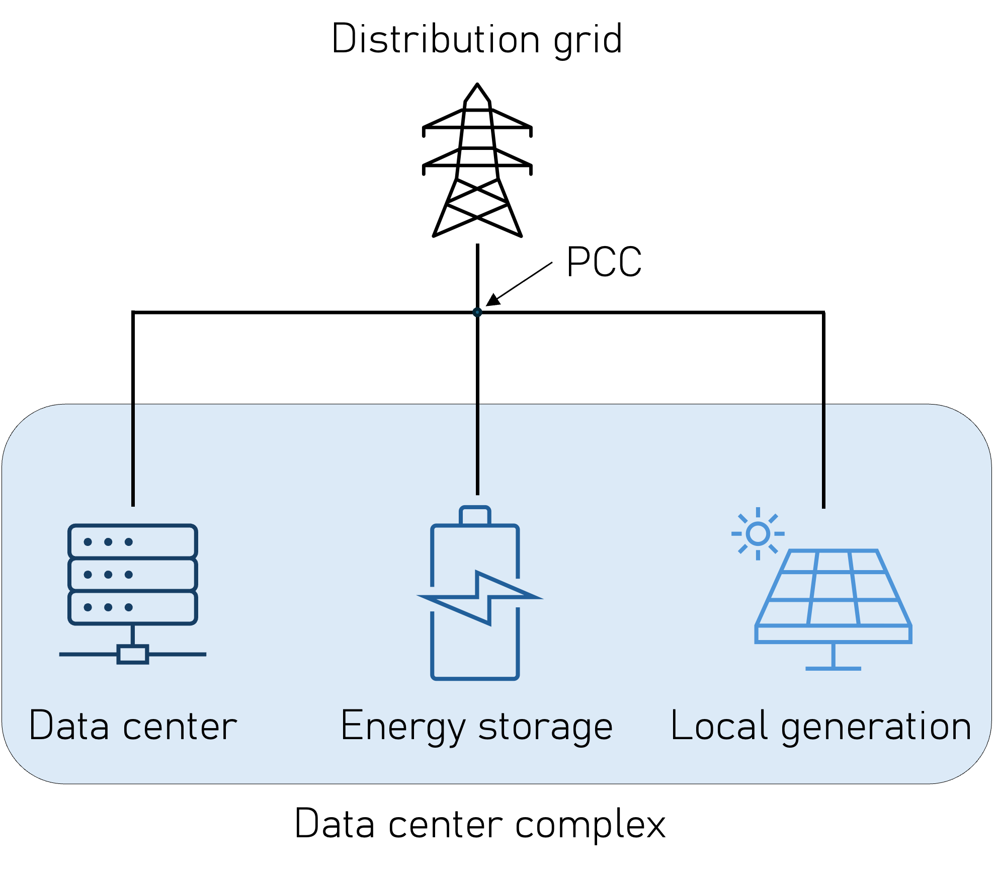
Figure 1: Schematic view of the resources configuration.

The method allows to consider the stochasticity of the data center demand, the solar irradiance, the carbon intensity of the imported electricity and the electricity tarifs, optimizing the system’s expected value of the carbon and financial cost over $N_{\text{tp}}^{\text{}}$ typical days with $N_{\text{sc}}^{\text{}}$ daily scenarios (for each stochastic quantity mentioned above).

2.1.2 Working hypotheses

The approach works with the following hypotheses:

• The data center complex (i.e., the data center and the associated DERs) is owned by a single entity: the DCO. This ensures that the resources can share common objectives, and allows for simple aggregation of investment and operational costs.

• The PV system can not be curtailed.

• The rated power at the Point of Common Coupling (PCC) is given (i.e., the DCO has an agreement in place with the power Distribution System Operator regarding the rating of the data center electricity supply).

• The efficiency of the ESS is assumed to be power independent and constant. This assumption is justified in planning problems whereas more sophisticated methods (such as those in [ollas_battery_2023]) may be considered in operational problems.

2.2 Problem formulation

A stochastic multi-objective convex minimisation problem with operational constraints is proposed. The problem determines the optimal ratings of the ESS and PV generation to minimize the expected value of an aggregated objective function, while ensuring the dispatchability of the data center complex. The objective function consists in the weighted sum of two objectives: the first aims at minimizing the carbon costs of the system (in $\text{\,}\mathrm{g}\mathrm{C}\mathrm{O}_{\mathrm{2}}\mathrm{e}\mathrm{q}$), while the latter targets the financial costs (in ¤, the generic currency symbol). Table˜1 summarizes the aspects that are considered in the objective function.

Carbon costs in $\text{\,}\mathrm{k}\mathrm{g}\mathrm{C}\mathrm{O}_{\mathrm{2}}\mathrm{e}\mathrm{q}$	Financial costs in ¤
The emissions from grid electricity imports	Electricity bill
ESS equivalent emissions	ESS investment, operation and maintenance
Generation equivalent emissions	Generation investment, operation and maintenance

Table 1: Components of the multi-objective function.

The optimization process is performed under multiple operational constraints on the ESS dynamics, aging, efficiency and ratings, on the PV generation aging and ratings, as well as on the grid connection capacity. The problem aims at minimizing the expected value of the objective function, over $N_{\text{tp}}^{\text{}}$ time horizons of $W$ hours each, and over $N_{\text{sc}}^{\text{}}$ scenarios per time horizon. For every time horizon, the problem computes an optimal dispatch plan (i.e., $P_{\text{pcc}}^{\text{}}(t)$, for $t\in[0,W]$) that is feasible for all the scenarios generated for that particular horizon. In other words, the sizing computes a dispatch plan for $N_{\text{tp}}^{\text{}}$ $W$-long time horizons. In this paper, a $W=$24\text{\,}\mathrm{h}$$ time horizon is used, since it is a typical dispatching use-case due to the structure of the electricity market [sossan_achieving_2016, gupta_coordinated_2022].

2.3 Mathematical model

2.3.1 Local glossary

The parameters used in the optimization problem are listed in this section. Note that $N$ is the number of discrete time steps in the time horizon $W$ (i.e., the number of steps in a typical day) and $\Delta T$ is the duration of a time step (thus, $W=N\cdot\Delta T$ is the length of the horizon in hours). $M$ is the product of $N_{\text{tp}}^{\text{}}$ and $N_{\text{sc}}^{\text{}}$; it corresponds to the total number of scenarios considered in the sizing problem. Matrices are highlighted in bold and, for a given matrix $\textbf{M}_{\text{}}^{\text{}}$, the entry at row $i$ and column $j$ is referred to as $\textbf{M}_{\text{}}^{\text{}}[i][j]$. The decision variables are the power profile of the storage system ($\textbf{P}_{\text{ess}}^{\text{}}\in\mathbb{R}^{N\times M}$), the rated capacity of the storage system ($E_{\text{rated}}^{\text{ess}}\in\mathbb{R}$) and the rated power of the PV generation system ($P_{\text{rated}}^{\text{gen}}\in\mathbb{R}$). To enhance readability, the other variables are only listed with their nature and dimensions. If their meaning is not clear, the reader can refer to the glossary in Declaration of competing interest.

• Auxiliary variables:

  • $\textbf{E}_{\text{ess}}^{\text{}}\in\mathbb{R}^{(N+1)\times M}$

  • $\textbf{P}_{\text{pcc}}^{\text{}}$, $\textbf{P}_{\text{gen}}^{\text{}}$, $\textbf{P}_{\text{ess}}^{\text{conv}}$, $\textbf{P}_{\text{ess}}^{\text{charge}}$, $\textbf{P}_{\text{ess}}^{\text{discharge}}$, $\textbf{z}_{\text{ess}}^{\text{}}$, $\textbf{P}_{\text{pcc}}^{\text{load}}$, $\textbf{P}_{\text{pcc}}^{\text{gen}}$, $\textbf{z}_{\text{pcc}}^{\text{}}\in\mathbb{R}^{N\times M}$

  • $\textbf{P}_{\text{pcc}}^{\text{dispatch}}\in\mathbb{R}^{N\times N_{\text{tp}}^{\text{}}}$

  • $\textbf{P}_{\text{pcc}}^{\text{max}}\in\mathbb{R}^{1\times M}$

  • $P_{\text{ess}}^{\text{rated}}$, $E_{\text{ess}}^{\text{start}}$, $E_{\text{ess}}^{\text{min}}$, $E_{\text{ess}}^{\text{max}}$, $C_{\text{e}}^{\text{pcc}}$, $C_{\text{e}}^{\text{ess}}$, $C_{\text{e}}^{\text{gen}}$, $c_{\text{ess}}^{\text{}}$, $c_{\text{gen}}^{\text{}}$, $c_{\text{el}}^{\text{energy}}$, $c_{\text{el}}^{\text{power}}\in\mathbb{R}$

• Inputs:

  • $\textbf{P}_{\text{load}}^{\text{}}$, $\textbf{i}_{\text{ghi}}^{\text{}}$, $\textbf{C}_{\text{i}}^{\text{pcc}}$, $\textbf{p}_{\text{el}}^{\text{cons}}$, $\textbf{p}_{\text{el}}^{\text{inj}}\in\mathbb{R}^{N\times M}$

  • $N_{\text{}}^{\text{}}$, $M_{\text{}}^{\text{}}$, $N_{\text{tp}}^{\text{}}$, $N_{\text{sc}}^{\text{}}$, $\Delta T$, $W$, $w$, $P_{\text{pcc}}^{\text{rated}}$, $C_{\text{i}}^{\text{ess}}$, $C_{\text{e, LCA}}^{\text{ess}}$, $r_{\text{ess}}^{\text{p2e}}$, $r_{\text{gen}}^{\text{ghi2p}}$, $i_{\text{ghi}}^{\text{max}}$, $\textit{SoC}_{\text{ess}}^{\text{min}}$, $\textit{SoC}_{\text{ess}}^{\text{max}}$, $\textit{SoC}_{\text{ess}}^{\text{start}}$, $L_{\text{ess}}^{\text{cycles}}$, $L_{\text{ess}}^{\text{calendar}}$, $L_{\text{gen}}^{\text{calendar}}$, $c_{\text{ess}}^{\text{energy}}$, $c_{\text{ess}}^{\text{power}}$, $c_{\text{gen}}^{\text{power}}$, $p_{\text{el}}^{\text{power}}$, $\eta_{\text{ess}}^{\text{}}$, $M_{\text{ess}}^{\text{}}$, $M_{\text{pcc}}^{\text{}}\in\mathbb{R}$

Also, note that, in the following, inequalities between a matrix and a scalar (e.g., $\textbf{V}\geq s$) mean that all entries of the matrix must satisfy the inequality (e.g., all entries of V are larger or equal to $s$).

2.3.2 Formulation

The proposed objective function $F_{\text{obj}}^{\text{}}$ is given in (1), where the symbols $C_{\text{x}}^{\text{y}}$ represent the carbon costs, and the symbols $c_{\text{x}}^{\text{y}}$ the financial costs. The weight $w$ in $\text{\,}\mathrm{g}\mathrm{C}\mathrm{O}_{\mathrm{2}}\mathrm{e}\mathrm{q}\mathrm{/}$¤ ponders the two objectives.

$$F_{\text{obj}}^{\text{}}\left(\textbf{P}_{\text{ess}}^{\text{}},E_{\text{ess}}^{\text{rated}},P_{\text{gen}}^{\text{rated}}\right)=C_{\text{e}}^{\text{pcc}}+C_{\text{e}}^{\text{ess}}+C_{\text{e}}^{\text{gen}}+w\cdot\left(c_{\text{ess}}^{\text{}}+c_{\text{gen}}^{\text{}}+c_{\text{el}}^{\text{energy}}+c_{\text{el}}^{\text{power}}\right)$$ (1)

In (2), $\mathcal{O}$ is used to denote the set of operational constraints (i.e., the physical constraints considered in the sizing problem). For instance, (2a) limits the ESS power to its rated values, while the energy contained in the ESS is constrained by (2b), which forces a predefined energy to be stored at the start of every day in the optimization time window. (2c) sets the lower and upper bounds for the energy stored in the system. Constraint (2d) links the energy stored in the ESS with its power. The power limit at the point of common coupling is set through (2e) and the power at the PCC is computed in (2f) (note that the assumption that losses can be neglected is made). Finally, (2g) ensures that the rated power of the generation is a positive number.

$$\mathcal{O}=[ -P_{\text{ess}}^{\text{rated}}\leq\textbf{P}_{\text{ess}}^{\text{conv}}\leq P_{\text{ess}}^{\text{rated}},$$ (2a)

$$\textbf{E}_{\text{ess}}^{\text{}}[0][j]=E_{\text{ess}}^{\text{start}},~\text{for }[j\in\mathbb{N}:0\leq j\leq M-1],$$ (2b)

$$E_{\text{ess}}^{\text{min}}\leq\textbf{E}_{\text{ess}}^{\text{}}\leq E_{\text{ess}}^{\text{max}},$$ (2c)

$$\textbf{E}_{\text{ess}}^{\text{}}[k+1][j]=\textbf{E}_{\text{ess}}^{\text{}}[k][j]+T\cdot\textbf{P}_{\text{ess}}^{\text{}}[k][j],~\text{for }[k\in\mathbb{N}:0\leq k\leq N-1],~\text{and }[j\in\mathbb{N}:0\leq j\leq M-1],$$ (2d)

$$-P_{\text{pcc}}^{\text{rated}}\leq\textbf{P}_{\text{pcc}}^{\text{}}\leq P_{\text{pcc}}^{\text{rated}},$$ (2e)

$$\textbf{P}_{\text{pcc}}^{\text{}}=\textbf{P}_{\text{ess}}^{\text{conv}}+\textbf{P}_{\text{load}}^{\text{}}-\textbf{P}_{\text{gen}}^{\text{}},$$ (2f)

$$P_{\text{rated}}^{\text{gen}}\geq 0]$$ (2g)

In (3), $\mathcal{A}$ is the set of auxiliary constraints (i.e., the artificial constraints used to formulate the problem). Constraints (3a), (3b) and (3c) link the user defined parameters $\textit{SoC}_{\text{ess}}^{\text{min/max/start}}$ and their equivalent stored energies, which are then used in constraints (2b) and (2c). Constraint (3d) ensures that the ESS acts like a buffer of energy, which does not, on average and for all typical time horizons, get charged nor discharged. Moreover, (3e) to (3j) are used to recover the generation and consumption components of the PCC dispatches: (3e) ensures that the sum of those components is equal to the PCC power, while (3f), (3g), (3h), (3i) and (3j) ensure that at least one of $\textbf{P}_{\text{pcc}}^{\text{load}}$ and $\textbf{P}_{\text{pcc}}^{\text{gen}}$ is equal to zero at any timestep of any scenario. Similarly, (3k) to (3p) enable the splitting of the ESS power. More detail on the splitting of $\textbf{P}_{\text{pcc}}^{\text{dispatch}}$ (and $\textbf{P}_{\text{ess}}^{\text{}}$) is provided in Remark 2. Constraint (3q) links the storage power and the converter power through the efficiency of the system $\eta_{\text{ess}}^{\text{}}$. The constraint in (3r) forces a dependence between the energy and power ratings of the ESS through the user-defined parameter $r_{\text{ess}}^{\text{p2e}}$: this link is used to make the problem convex (in particular, it simplifies (4d) as detailed further below). Constraint (3s) ensures that the PCC power for every scenario of a given typical day is equal to the dispatch of that day (note that the transformation matrix $\textbf{T}_{\text{m}}^{\text{}}\in\mathbb{Z}_{2}^{M\times N_{\text{tp}}^{\text{}}}$ has to be built appropriately). Constraints (3t) and (3u) recover the maximum power consumption and generation of every typical day, so that they can be billed appropriately. Finally, the photovoltaic power is defined in (3v). Following [richardson_validation_2019], the power generation is modeled as a linear relationship between the solar irradiance [$\text{\,}\mathrm{W}\mathrm{/}\mathrm{m}^{2}$] and the plant peak power rating (defined at $i_{\text{ghi}}^{\text{max}}$ $\text{\,}\mathrm{W}\mathrm{/}\mathrm{m}^{2}$). Note that $r_{\text{gen}}^{\text{ghi2p}}\in[0,1]$ is a user-defined constant that can be used to adapt the slope of the linear relationship.

$$\mathcal{A}=[ \textit{SoC}_{\text{ess}}^{\text{min}}\cdot E_{\text{ess}}^{\text{rated}}=E_{\text{ess}}^{\text{min}},$$ (3a)

$$\textit{SoC}_{\text{ess}}^{\text{max}}\cdot E_{\text{ess}}^{\text{rated}}=E_{\text{ess}}^{\text{max}},$$ (3b)

$$\textit{SoC}_{\text{ess}}^{\text{start}}\cdot E_{\text{ess}}^{\text{rated}}=E_{\text{ess}}^{\text{start}},$$ (3c)

$$\sum_{k=0}^{N-1}\left(\textbf{P}_{\text{ess}}^{\text{}}\cdot\textbf{T}_{\text{m}}^{\intercal}\right)[k]=0,$$ (3d)

$$\textbf{P}_{\text{pcc}}^{\text{}}=\textbf{P}_{\text{pcc}}^{\text{load}}+\textbf{P}_{\text{pcc}}^{\text{gen}},$$ (3e)

$$\textbf{P}_{\text{pcc}}^{\text{load}}\geq 0,$$ (3f)

$$\textbf{P}_{\text{pcc}}^{\text{gen}}\leq 0,$$ (3g)

$$\textbf{P}_{\text{pcc}}^{\text{load}}\leq M_{\text{pcc}}^{\text{}}\cdot(1-\textbf{z}_{\text{pcc}}^{\text{}})$$ (3h)

$$-\textbf{P}_{\text{pcc}}^{\text{gen}}\leq M_{\text{pcc}}^{\text{}}\cdot\textbf{z}_{\text{pcc}}^{\text{}}$$ (3i)

$$0\leq\textbf{z}_{\text{pcc}}^{\text{}}\leq 1$$ (3j)

$$\textbf{P}_{\text{ess}}^{\text{}}=\textbf{P}_{\text{ess}}^{\text{charge}}+\textbf{P}_{\text{ess}}^{\text{discharge}},$$ (3k)

$$\textbf{P}_{\text{ess}}^{\text{charge}}\geq 0,$$ (3l)

$$\textbf{P}_{\text{ess}}^{\text{discharge}}\leq 0,$$ (3m)

$$\textbf{P}_{\text{ess}}^{\text{charge}}\leq M_{\text{ess}}^{\text{}}\cdot(1-\textbf{z}_{\text{ess}}^{\text{}})$$ (3n)

$$-\textbf{P}_{\text{ess}}^{\text{discharge}}\leq M_{\text{ess}}^{\text{}}\cdot\textbf{z}_{\text{ess}}^{\text{}}$$ (3o)

$$0\leq\textbf{z}_{\text{ess}}^{\text{}}\leq 1$$ (3p)

$$\textbf{P}_{\text{ess}}^{\text{conv}}=\textbf{P}_{\text{ess}}^{\text{charge}}/\eta_{\text{ess}}^{\text{}}+\eta_{\text{ess}}^{\text{}}\cdot\textbf{P}_{\text{ess}}^{\text{discharge}},$$ (3q)

$$P_{\text{ess}}^{\text{rated}}=r_{\text{ess}}^{\text{p2e}}\cdot E_{\text{ess}}^{\text{rated}},$$ (3r)

$$\textbf{P}_{\text{pcc}}^{\text{}}=\textbf{P}_{\text{pcc}}^{\text{dispatch}}\cdot\textbf{T}_{\text{m}}^{\text{}},$$ (3s)

$$\textbf{1}^{N\times 1}\cdot\textbf{P}_{\text{pcc}}^{\text{max}}\geq\textbf{P}_{\text{pcc}}^{\text{load}},$$ (3t)

$$\textbf{1}^{N\times 1}\cdot\textbf{P}_{\text{pcc}}^{\text{max}}\geq-\textbf{P}_{\text{pcc}}^{\text{gen}},$$ (3u)

$$\textbf{P}_{\text{gen}}^{\text{}}=\frac{r_{\text{gen}}^{\text{ghi2p}}P_{\text{gen}}^{\text{rated}}}{i_{\text{ghi}}^{\text{max}}}\cdot\textbf{i}_{\text{ghi}}^{\text{}}]$$ (3v)

$\mathcal{F}$, in (4), gives the set of constraints used to compute the expected daily costs of the system. In the set, $j\in[j:0\leq j<M]$ is the index over the typical days and scenarios, while $k\in[k:0\leq k<N]$ is the index over the steps in typical days. Constraints (4a), (4b) and (4c) model the expected carbon costs of the ESS, the generation and the PCC respectively.

$$\mathcal{F}=[ C_{\text{e}}^{\text{ess}}=\frac{\Delta T\cdot C_{\text{i}}^{\text{ess}}}{M}\cdot\sum_{j=0}^{M-1}\sum_{k=0}^{N-1}\left|\textbf{P}_{\text{ess}}^{\text{}}[k][j]\right|+E_{\text{ess}}^{\text{rated}}\frac{W\cdot C_{\text{e, LCA}}^{\text{ess}}}{L_{\text{ess}}^{\text{calendar}}},$$ (4a)

$$C_{\text{e}}^{\text{gen}}=\frac{W}{L_{\text{gen}}^{\text{calendar}}}\cdot P_{\text{rated}}^{\text{gen}}\cdot C_{\text{e, LCA}}^{\text{gen}},$$ (4b)

$$C_{\text{e}}^{\text{pcc}}=\frac{\Delta T}{M}\cdot\sum_{j=0}^{M-1}\sum_{k=0}^{N-1}\textbf{C}_{\text{i}}^{\text{pcc}}[k][j]\cdot\textbf{P}_{\text{pcc}}^{\text{load}}[k][j],$$ (4c)

$$c_{\text{ess}}^{\text{}}=\left(\frac{E_{\text{ess}}^{\text{rated}}\cdot W}{L_{\text{ess}}^{\text{calendar}}}+\frac{\Delta T}{2\cdot L_{\text{ess}}^{\text{cycles}}\cdot M}\sum_{j=0}^{M-1}\sum_{k=0}^{N-1}\left|\textbf{P}_{\text{ess}}^{\text{}}[k][j]\right|\right)\cdot\left(c_{\text{ess}}^{\text{energy}}+c_{\text{ess}}^{\text{power}}\cdot r_{\text{ess}}^{\text{p2e}}\right),$$ (4d)

$$c_{\text{gen}}^{\text{}}=\frac{W}{L_{\text{gen}}^{\text{calendar}}}\cdot P_{\text{gen}}^{\text{rated}}\cdot c_{\text{gen}}^{\text{power}},$$ (4e)

$$c_{\text{el}}^{\text{energy}}=\frac{\Delta T}{M}\cdot\sum_{j=0}^{M-1}\sum_{k=0}^{N-1}\textbf{p}_{\text{el}}^{\text{cons}}[k][j]\cdot\textbf{P}_{\text{pcc}}^{\text{load}}[k][j]+\textbf{p}_{\text{el}}^{\text{inj}}[k][j]\cdot\textbf{P}_{\text{pcc}}^{\text{gen}}[k][j],$$ (4f)

$$c_{\text{el}}^{\text{power}}=\frac{1}{M}\sum_{j=0}^{M-1}p_{\text{el}}^{\text{power}}\cdot\textbf{P}_{\text{pcc}}^{\text{max}}[j]\cdot W_{\text{days}}^{\text{}}]$$ (4g)

In (4a), emissions are modeled by superposing the ESS cycling-based and calendar-based aging [schmalstieg_holistic_2014]. In the context of Life Cycle Assessments (LCA) for energy storage systems, $C_{\text{e, LCA}}^{\text{ess}}$ estimates the $\text{\,}\mathrm{g}\mathrm{C}\mathrm{O}_{\mathrm{2}}\mathrm{e}\mathrm{q}$ emitted to install a kilowatt-hour of storage and is used to account for the carbon emissions related to the calendar aging of the asset via Eq.˜5, which assumes that the calendar aging of the ESS is linear.

$$C_{\text{e, cal}}^{\text{ess}}=\frac{W}{L_{\text{ess}}^{\text{calendar}}}\cdot E_{\text{ess}}^{\text{rated}}\cdot C_{\text{e, LCA}}^{\text{ess}}$$ (5)

To further account for the effects of cycling-based aging (e.g., for battery storage systems), the term $C_{\text{i}}^{\text{ess}}$ (6a) is introduced, which quantifies the carbon emissions per $\text{\,}\mathrm{kW}\text{\,}\mathrm{h}$ of energy throughput. Cycling-based aging is assumed to be linearly growing with the ESS energy throughput $\textbf{E}_{\text{throughput}}^{\text{ess}}$, which is formulated in (6b).

$$C_{\text{i}}^{\text{ess}} =\frac{C_{\text{e, LCA}}^{\text{ess}}}{2\cdot L_{\text{ess}}^{\text{cycles}}}$$ (6a)

$$\textbf{E}_{\text{throughput}}^{\text{ess}}[j] =T\cdot\sum_{k=0}^{N-1}\left|\textbf{P}_{\text{ess}}^{\text{}}[k][j]\right|\text{, for }0\leq j<M$$ (6b)

Similarly to Eq.˜5, the emissions of the generation asset are estimated in (4b) using its life cycle assessment. $C_{\text{e, LCA}}^{\text{gen}}$, which estimates the $\text{\,}\mathrm{g}\mathrm{C}\mathrm{O}_{\mathrm{2}}\mathrm{e}\mathrm{q}$ emitted to install a kilowatt of photovoltaic generation peak power. The carbon emissions related to the grid imports (i.e., $\textbf{P}_{\text{pcc}}^{\text{load}}$) are computed in (4c) using the carbon intensity of the imported electricity $\textbf{C}_{\text{i}}^{\text{pcc}}$ [$\text{\,}\mathrm{g}\mathrm{C}\mathrm{O}_{\mathrm{2}}\mathrm{e}\mathrm{q}\mathrm{/}\mathrm{k}\mathrm{W}\mathrm{h}$]. Finally, (4d) to (4g) are used to model the expected financial costs of the system. The cost of the ESS is expressed in (4d), which considers both the calendar-based and cycling-based aging processes. The financial cost of installing a $\text{\,}\mathrm{kW}\text{\,}\mathrm{h}$ of storage capacity is denoted by $c_{\text{ess}}^{\text{energy}}$, and the financial cost of installing a $\text{\,}\mathrm{kW}$ of storage power is denoted by $c_{\text{ess}}^{\text{power}}$. Over the lifetime of the storage system, its cost $c_{\text{ess}}^{\text{life}}$ is computed in Eq.˜8. This cost is scaled to the average amount of aging (i.e., $a_{\text{ess}}^{\text{}}$) of the system during the optimization time window, which is computed in Eq.˜9. To make the constraint on $c_{\text{ess}}^{\text{}}$ convex, the input parameter $r_{\text{ess}}^{\text{p2e}}$ in Eq.˜7 is introduced. The equivalent financial cost is expressed via the multiplication $c_{\text{ess}}^{\text{life}}$ and $a_{\text{ess}}^{\text{}}$, while replacing the occurrences of $P_{\text{ess}}^{\text{rated}}$ with $r_{\text{ess}}^{\text{p2e}}E_{\text{ess}}^{\text{rated}}$. More considerations on $r_{\text{ess}}^{\text{p2e}}$ can be found in Remark 3.

$$r_{\text{ess}}^{\text{p2e}}=\frac{P_{\text{ess}}^{\text{rated}}}{E_{\text{ess}}^{\text{rated}}}$$ (7)

$$c_{\text{ess}}^{\text{life}}=c_{\text{ess}}^{\text{energy}}\cdot E_{\text{ess}}^{\text{rated}}+c_{\text{ess}}^{\text{power}}\cdot P_{\text{ess}}^{\text{rated}}$$ (8)

$$a_{\text{ess}}^{\text{}}=W/L_{\text{ess}}^{\text{calendar}}+\frac{\sum_{j=0}^{M-1}\sum_{k=0}^{N-1}\left|\textbf{P}_{\text{ess}}^{\text{}}[k][j]\right|}{2\cdot E_{\text{ess}}^{\text{rated}}\cdot L_{\text{ess}}^{\text{cycles}}\cdot M}$$ (9)

The financial cost of the generation asset is considered in (4e), which is identical to (4b) but in financial terms. Lastly, the electricity bill is estimated in (4f) and (4g). The first models the cost related to the energy consumption and production at the PCC (with prices per $\text{\,}\mathrm{kW}\text{\,}\mathrm{h}$ set through $\textbf{p}_{\text{el}}^{\text{cons}}$ and $\textbf{p}_{\text{el}}^{\text{inj}}$), while the second models the cost related to the maximum $15\text{\,}\mathrm{min}$ average power consumption. Although the maximum power is typically billed monthly or yearly, the worst case scenario over the optimization time window is used (which is equivalent to assuming one power bill per dispatch). Note that $p_{\text{el}}^{\text{power}}$ must thus often be recomputed (e.g., if the consumption site billing scheme bills $p_{\text{el}}^{\text{power, month}}$ for each $\text{\,}\mathrm{kW}$ of monthly peak power, then $p_{\text{el}}^{\text{power}}=\frac{12}{365}p_{\text{el}}^{\text{power, month}}$). Combining Eq.˜1, Eq.˜2, Eq.˜3, and Eq.˜4, the sizing optimization problem is formulated in Eq.˜10.

$$\min_{E_{\text{ess}}^{\text{rated}},~P_{\text{gen}}^{\text{rated}},~\textbf{P}_{\text{ess}}^{\text{}}} F_{\text{obj}}^{\text{}}$$ (10)

s.t. $$\mathcal{O}\cup\mathcal{A}\cup\mathcal{F}$$

2.4 A few guidelines and remarks on the method

As mentioned in the above, the method enables to consider the carbon and financial cost of the system, although the user is free to leverage this feature or not (i.e., by manipulating the inputs of the problem). Similarly, the method considers the stochastic nature of the consumption, the irradiance and the carbon intensity of the grid. However, the user can run the problem with $N_{\text{sc}}^{\text{}}=N_{\text{tp}}^{\text{}}=1$ and perform a deterministic sizing of the resources. Note that in reality, the optimal sizing depends on the control scheme that will be applied to the system, as well as on the forecasting methods that will be used. To guarantee the coherence between the sizing of the resources and their operation, the user has to use the same forecasting methods and operational objectives adopted in the sizing stage.

Remark 1.

The weight $w$, in $\text{\,}\mathrm{g}\mathrm{C}\mathrm{O}_{\mathrm{2}}\mathrm{e}\mathrm{q}\mathrm{/}$¤, balances the trade-off between minimizing carbon emissions and minimizing costs. It represents the amount of $\text{\,}\mathrm{g}\mathrm{C}\mathrm{O}_{\mathrm{2}}\mathrm{e}\mathrm{q}$ that need to be saved to justify a unit increase of the operational cost of the system. In Eq.˜11, the objective function (1) is divided by $w$ to provide its simpler and clearer interpretation. Indeed, the inverse of $w$ represents the financial cost of an emitted $\text{\,}\mathrm{g}\mathrm{C}\mathrm{O}_{\mathrm{2}}\mathrm{e}\mathrm{q}$. Therefore, users of the sizing tool can appropriately set $w$ according to preliminary studies on the value of a saved gram of carbon dioxide equivalents. The studies should consider the local policies (such as carbon taxes) and/or company-specific policies.

$$\frac{1}{w}F_{\text{obj}}^{\text{}}\left(P_{\text{ess}}^{\text{rated}},E_{\text{ess}}^{\text{rated}},P_{\text{gen}}^{\text{rated}}\right)=\frac{1}{w}\left(C_{\text{e}}^{\text{pcc}}+C_{\text{e}}^{\text{ess}}+C_{\text{e}}^{\text{gen}}\right)+c_{\text{ess}}^{\text{}}+c_{\text{gen}}^{\text{}}+c_{\text{el}}^{\text{energy}}+c_{\text{el}}^{\text{power}}$$ (11)

Remark 2.

$\textbf{P}_{\text{pcc}}^{\text{}}$ is split in $\textbf{P}_{\text{pcc}}^{\text{load}},~\textbf{P}_{\text{pcc}}^{\text{gen}}$ to enable different policies for the carbon and financial costs at the PCC, depending on whether the PCC is exporting or importing power. The application of the policies can be observed in the constraints for $C_{\text{e}}^{\text{pcc}}$ and $c_{\text{el}}^{\text{energy}}$ (4c and 4f). However, for the optimal solution of the problem to be relevant, $\textbf{P}_{\text{pcc}}^{\text{load}},~\textbf{P}_{\text{pcc}}^{\text{gen}}$ must be exclusive, meaning that at least one of them must be equal to zero at every timestep (i.e., power can not be imported and exported at the same time). This relation is guaranteed through constraints (3e) to (3j), using the continuous indicator variable $\textbf{z}_{\text{pcc}}^{\text{}}$ and the large-enough constant $M_{\text{pcc}}^{\text{}}$. Note that the battery power $\textbf{P}_{\text{ess}}^{\text{}}$ is also split in two parts to enable the accounting of the efficiency of the system (3q). The exclusivity of the two variables $\textbf{P}_{\text{ess}}^{\text{charge}}$ and $\textbf{P}_{\text{ess}}^{\text{discharge}}$ is guaranteed in the same way.

Remark 3.

The parameter $r_{\text{ess}}^{\text{p2e}}$ (defined in Eq.˜7) is used to convexify constraint Eq.˜4d. This reduces the set of possible ESS ratings to those with a fixed power to energy ratio. To get an idea on how this ratio impacts the sizing process, the sizing problem can be solved multiple times with different ratios.

Remark 4.

Note that in many cases, some of the equality constraints in the problem might have to be relaxed (either for computational reasons or to make the problem feasible). For example, constraint (3d) can be relaxed by replacing it by the two constraints $-\epsilon\leq\sum_{j=0}^{M-1}\sum_{k=0}^{N-1}\textbf{P}_{\text{ess}}^{\text{}}[k][j]\leq\epsilon$, where $\epsilon$ is a small-enough positive number chosen by the user. Similarly, constraint (3s) can be relaxed by replacing it with constraints (12a) and (12b), which results in setting a $\epsilon_{\text{t}}^{\text{}}$ dispatch-tracking accuracy. Constraint (12c) computes the dispatch plans as the expected value of the PCC power profile of each typical day.

$$\textbf{P}_{\text{pcc}}^{\text{}}\geq\textbf{P}_{\text{pcc}}^{\text{dispatch}}\cdot\textbf{T}_{\text{m}}^{\text{}}-\epsilon_{\text{t}}^{\text{}},$$ (12a)

$$\textbf{P}_{\text{pcc}}^{\text{}}\leq\textbf{P}_{\text{pcc}}^{\text{dispatch}}\cdot\textbf{T}_{\text{m}}^{\text{}}+\epsilon_{\text{t}}^{\text{}},$$ (12b)

$$\textbf{P}_{\text{pcc}}^{\text{}}\cdot\textbf{T}_{\text{m}}^{\intercal}=N_{\text{sc}}^{\text{}}\cdot\textbf{P}_{\text{pcc}}^{\text{dispatch}},$$ (12c)

3 Case study: data and implementation context

3.1 Implementation

The method presented in Section 2 is implemented using Jupyter Notebooks with Python 3.11.8. The cvxpy library [diamond_cvxpy_nodate] is used to formulate the problem and license based GUROBI is used to solve it. License-free solvers (e.g., CLARABEL) that are natively supported by cvxpy can also be used, although they might be less efficient and/or produce less accurate solutions.

3.2 Data availability

This section provides a description of the data used in this research, with references.

3.2.1 Data center consumption

Publicly available data from [wilkes_yet_2020] is used to model the consumption of the servers. The dataset contains a month of data (i.e., may 2019), with $5\text{\,}\mathrm{min}$ granularity for  50 Power Distribution Units (PDUs), each PDU reports data in per units. The PDUs are aggregated in cells. Cell A is selected arbitrarily and the power attributed to production workloads [sakalkar_data_2020] (i.e., the production_power_util field) of all the power distribution units in that cell (assuming every PDU in the cell has the same power rating) is aggregated. The aggregated data is then scaled up to a selected installed power.

3.2.2 Grid carbon intensity

The grid carbon intensity data utilized in this study comes from a start-up specializing in solutions to monitor the cleanliness of electricity. More documentation can be found in [emissium_emissium_nodate]. In particular, the start-up provides tools capable of tracking the Global Warming Potential over 100 years (GWP100) of a $\text{\,}\mathrm{kW}\text{\,}\mathrm{h}$ with a $15\text{\,}\mathrm{min}$ time granularity in different NUTS levels (Nomenclature of Territorial Units for Statistics). In this research, swiss cantonal data for the year 2023 is leveraged along with the data of german first level NUTS, enabling detailed analysis and insights into the temporal (and geographical) variations of carbon intensity in the german and swiss electricity grid.

3.2.3 Electricity prices

The day-ahead market prices come from the ENTSOE transparency platform, for year 2023 [entsoe_day-ahead_2023]. Since day-ahead market prices are used, the injection and consumption tariffs are the same and the power price is not considered (i.e., is set to zero). Note that for different billing schemes (s.a. [romande_energie_tarifs_2024]), the injection and consumption tariffs might be different and a power tariff might need to be incorporated.

3.2.4 Irradiance

Historical data for the locations under study is recovered from the Copernicus Atmosphere Monitoring Service (CAMS). The data covers year 2023 and was accessed in August 2024 [copernicus_atmosphere_monitoring_service_cams_cams_nodate, qu_fast_2017, schroedter-homscheidt_surface_2022].

3.2.5 ESS and PV inputs

The life-cycle footprint (GWP100) of the storage and photovoltaic system are recovered from the Ecoinvent database [wernet_ecoinvent_2016]. In particular, the LCA values for the production of Li-ion LiMn2O4 batteries (reported in [dominic_notter_battery_nodate]) and for the flat-roof installation of multi-Si PV systems in Switzerland (reported in [niels_jungbluth_photovoltaic_nodate]) are used. The financial cost of a battery installation is recovered from [yi_dispatch-aware_2023], and the financial cost of a PV installation is recovered from [christian_bauer_potentials_2017]. The study cases focus on battery storage systems because their high round-trip efficiency and their fast response time make them particularly well suited for short-term applications (such as day-ahead dispatching).

3.3 Generation of scenarios

Although forecasting stochastic variables is not the focal point of this paper, addressing scenario generation is essential to effectively study the method. In this paper, a combination of clustering and random sub-sampling (i.e., Monte Carlo simulations [glasserman_monte_2010]) is used to generate scenarios. Specifically, seasonal clustering and weekday/weekend clustering are applied for the load, day-ahead prices and carbon emissions, as well as seasonal and energy-based clustering for the irradiance. Irradiance observations within a given season are grouped into three clusters based on their surface energy content (i.e., the integral of the irradiance over a day) using K-Means [lloyd_least_1982]. The typical days to be considered by the sizing problem are selected so that they maintain the ratios between the populations of these clusters as accurately as possible. While respecting these ratios, a cluster is randomly assigned to every typical day. For the irradiance data, this step is valid under the assumption that information on the surface energy of the irradiance can be known day-ahead: it is reasonable to assume that information on the level of cloudiness of a day can be known 24$\text{\,}\mathrm{h}$ ahead.

3.4 Case study

The case of a 1 $\text{\,}\mathrm{MW}$ rated data center in different locations across Switzerland and Germany is studied. Switzerland, where this research is based, provides a unique context due to its energy mix, while Germany serves as a relevant comparative case given its geographical proximity to Switzerland and its radically different energy mix. Sizings are performed over 21 typical days per season (3 per day of the week) with 20 scenarios per typical day (i.e., $N_{\text{tp}}^{\text{}}=84,~N_{\text{sc}}^{\text{}}=20$), generating $M_{\text{}}^{\text{}}=1680$ scenarios per stochastic variable. This choice is detailed in LABEL:app:scenarios_number. Unless explicitly stated otherwise, a unitary power to energy ratio $r_{\text{ess}}^{\text{p2e}}=1$ is used.

4 Results

4.1 Single objective: carbon footprint reduction

For the first analysis of the method, the weight $w$ is set to 0 (i.e., the financial aspect of the problem is disregarded), and the case of the Neuchâtel Swiss canton is studied. Three levels of dispatch accuracy $\epsilon_{\text{t}}^{\text{}}$ are studied (leveraging Remark 4): $1\text{\,}\mathrm{kW}$, $10\text{\,}\mathrm{kW}$ and $100\text{\,}\mathrm{kW}$, corresponding to a power tracking error of 0.1%, 1% and 10% of the data center rated power. In Fig.˜2(a) and Fig.˜2(b), scenarios for a random typical day of the sizing process are shown. Fig.˜2(a) shows the computed dispatch (the dash-dot black line) as well as the PCC power profiles of every scenario and the average data center demand (the dashed red line), while Fig.˜2(b) shows the evolution of the battery state-of-charge. One can observe that the battery will discharge (i.e., the PCC power consumption is lower than the data center power demand) during the first hours of the day, because the carbon intensity is on a peak. Moreover, during the early morning hours, the battery starts to charge because the carbon content of the grid’s electricity during those hours is lower (Fig.˜2(c)). Then, the PCC demand lowers to avoid the higher grid carbon intensity hours (and to self-consume solar production), before going back up during late afternoon hours (where the carbon intensity is lower). It is worth noting the spread in the battery state-of-charge at the end of the day since, depending on the scenario, the battery has to follow different trajectories. On average, as imposed by Eq.˜3d, the battery acts like an energy buffer (as shown by the red dotted line, which shows the average SoC evolution).
The optimal capacity of the battery storage system is $4.9\text{\,}\mathrm{MW}\text{\,}\mathrm{h}$, $4.5\text{\,}\mathrm{MW}\text{\,}\mathrm{h}$ and $4.6\text{\,}\mathrm{MW}\text{\,}\mathrm{h}$ respectively. Since the power to energy ratio is equal to 1, the BESS power rating is $4.9\text{\,}\mathrm{MW}$, $4.5\text{\,}\mathrm{MW}$ and $4.6\text{\,}\mathrm{MW}$. For the PV system, the optimal power rating is $1.1\text{\,}\mathrm{MW}$, $1.1\text{\,}\mathrm{MW}$ and $1.3\text{\,}\mathrm{MW}$. These results appear very reasonable: the battery capacity is substantial because its carbon footprint is relatively low, allowing for carbon emission reductions via load shifting. Conversely, the PV system’s capacity is comparable to the data center rated power, and slightly increases with $\epsilon_{\text{t}}^{\text{}}$, as lower tracking accuracy allows for more stochasticity in the data center complex. Additionally, the battery rated capacity decreases when $\epsilon_{\text{t}}^{\text{}}$ increases as the battery is the only asset able to compensate the stochasticity in the system and, therefore, allowing for less precise tracking requires less BESS installation. It is worth noting that the choice of $\epsilon_{\text{t}}^{\text{}}$ is user-specific, as it allows the user to decide the importance of having a dispatchable system (i.e., large enough $\epsilon_{\text{t}}^{\text{}}$ will completely disregard the objective of achieving dispatchability). In the remainder of the paper, dispatchability is considered as a crucial aspect of the data center daily operations, given the current costs associated to imbalance prices in electricity. Therefore, a tracking accuracy of 0.1% is used.
In Fig.˜2(d), the Empirical Cumulative Distribution Function (ECDF) of the carbon emissions demonstrates that the method decreases the system’s Carbon Emissions (CE). The main reduction comes from high emission days, which are significantly reduced by the sizing process. Table˜2 shows that the sizing method reduces both the average daily emissions as well as their standard deviation.

Daily emissions	No ESS, no PV	$\epsilon_{\text{t}}^{\text{}}=$1\text{\,}\mathrm{kW}$$	$\epsilon_{\text{t}}^{\text{}}=$10\text{\,}\mathrm{kW}$$	$\epsilon_{\text{t}}^{\text{}}=$100\text{\,}\mathrm{kW}$$
Average in $\text{\,}\mathrm{t}\mathrm{C}\mathrm{O}_{\mathrm{2}}\mathrm{e}\mathrm{q}$	1.42	1.36	1.35	1.3
Standard dev. in $\text{\,}\mathrm{t}\mathrm{C}\mathrm{O}_{\mathrm{2}}\mathrm{e}\mathrm{q}$	0.87	0.75	0.75	0.68

Table 2: Metrics for daily carbon emissions, sizing with $w=0$.

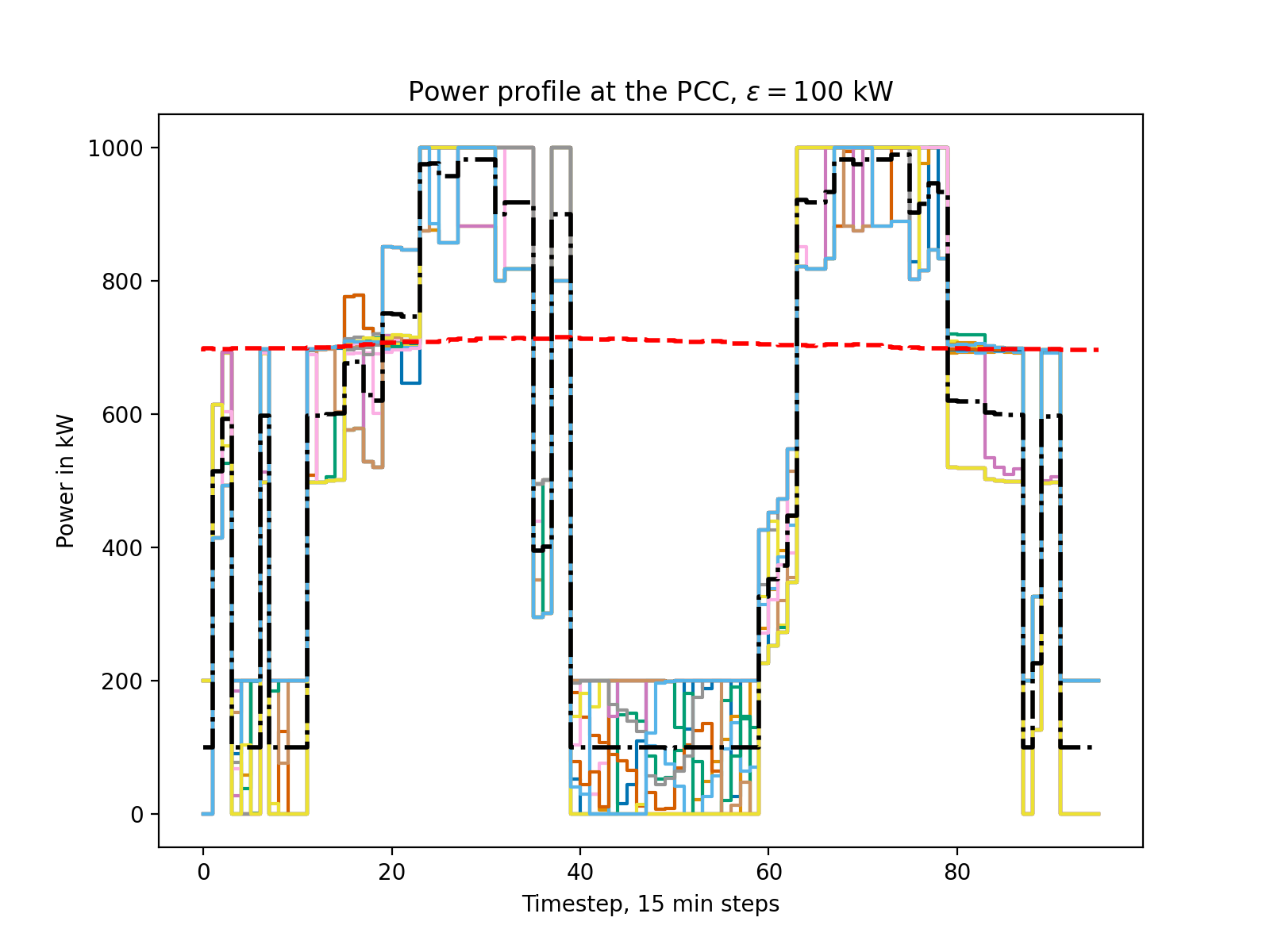
((a)) Dispatch and PCC power profiles.

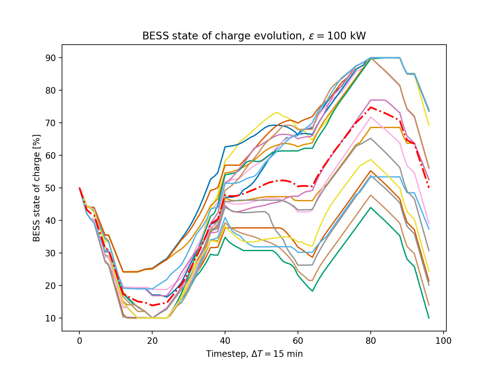
((b)) Evolution of the battery state of charge.

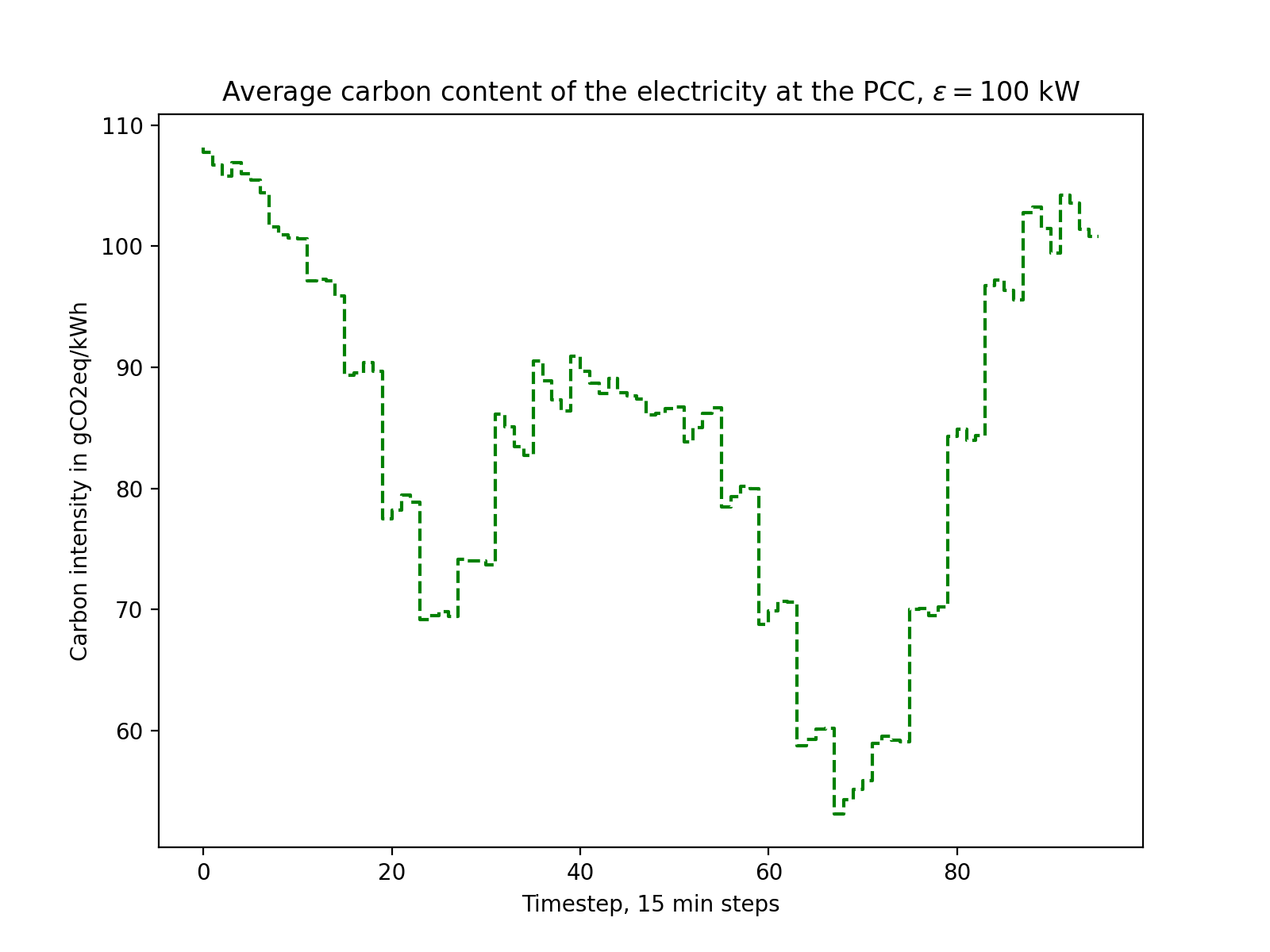
((c)) Average carbon intensity.

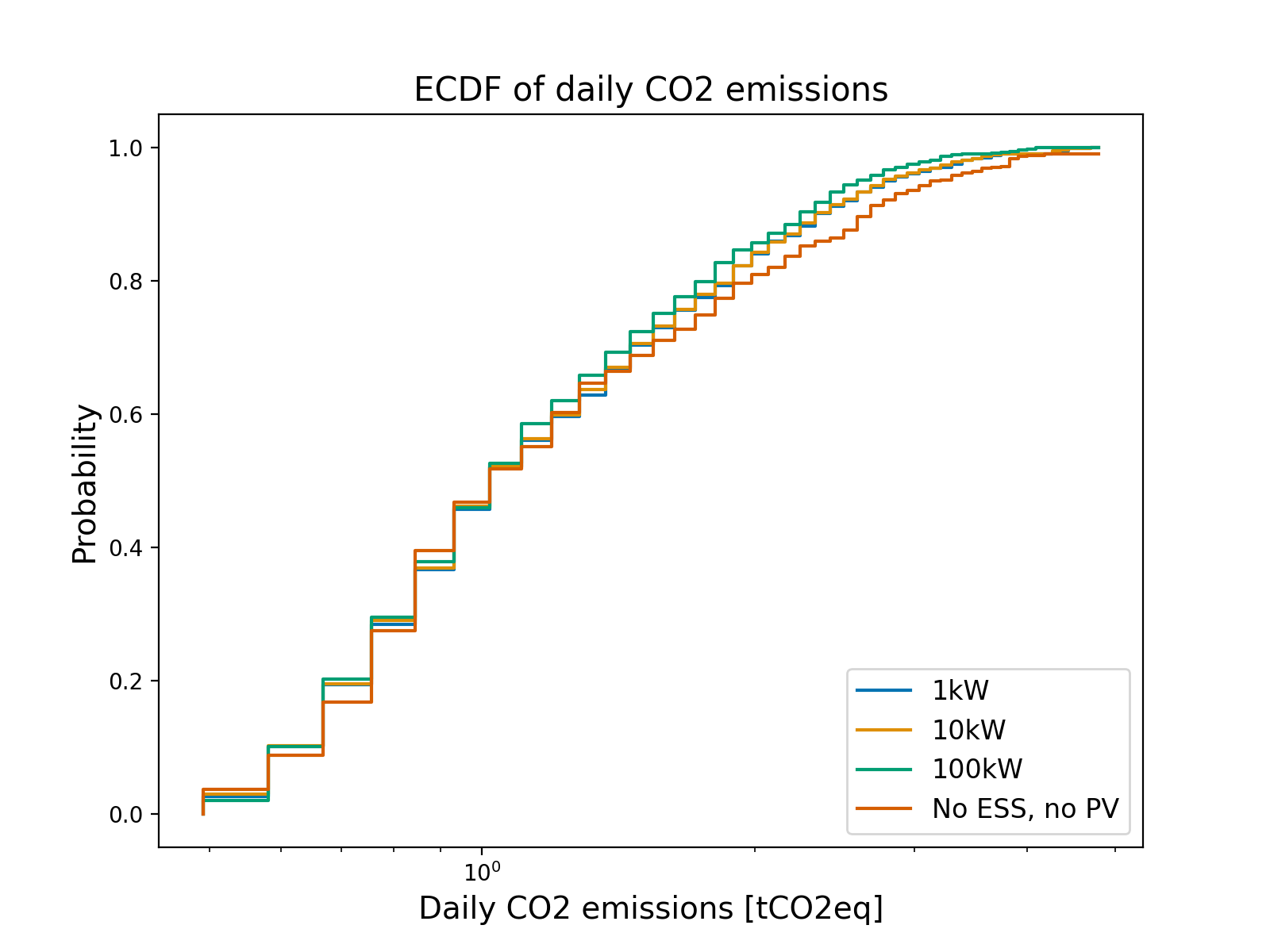
((d)) ECDF of the expected carbon emissions.

Figure 2: Results of a carbon-only sizing in Bayern (DE2)

4.2 Pareto front

In this section, the sensitivity of the sizing process to the weight $w$ is studied, for three Swiss cantons (i.e., Vaud-VD, Aargau-AG and Neuchâtel-NE) and two NUTS1 areas of Germany (i.e., Bayern-DE2 and Schleswig-Holstein-DEF). Aargau and Neuchâtel are selected as they are the Swiss cantons with lowest and highest average grid carbon intensity respectively (as shown in LABEL:fig:ci_cantonal), while the average of canton Vaud is close to the Swiss average grid carbon intensity. Bayern and Schleswig-Holstein are selected to represent the northern and southern part of Germany. In this context, the evolution of the ESS and PV ratings, as well as the evolution of the carbon and financial objectives are shown in Fig.˜3.

4.2.1 Evolution of the objectives

By focusing on the plots on the right side of Fig.˜3, the impact of the weight (i.e., $w$) on the sizing objectives can be studied. As a reminder, the objectives are the reduction of the system’s carbon footprint and of the system’s costs, as detailed in Eq.˜1. As expected, increasing the weight tends to increase carbon emissions while reducing costs. This happens because larger weights indicate that the DCO puts the emphasis on the economic aspect of the system operation, therefore prioritizing cost savings over carbon savings. In Fig.˜3, the black dotted lines show the expected daily objectives for the base case (i.e., for the operation of the data center alone; without PV, without BESS and without demand side control). The base case expected carbon emissions for the different regions are significantly different as the historical carbon intensity of the electricity consumed in each region varies, and the carbon saving opportunities strongly depend on the base case carbon emissions. In fact, the maximum expected footprint reduction (i.e., the reduction when $w=0$) is approximately 49.6% for a sizing in the Bayern region, 14.7% in Schleswig-Holstein, 4% in canton Neuchâtel, 0.3% for canton Vaud and -2.6% for canton Aargau. It is interesting to observe that for a region in which the carbon intensity of the consumed electricity is very low (such as Aargau), the underlying constraint of achieving the dispatchability of the system (i.e. being able to track a day-ahead consumption plan) increases the expected carbon emissions of the system, even if the sizing is performed with the carbon footprint objective only. In terms of costs, sizing the DERs using low weights can increase the operational costs significantly (e.g., the $w=0$ sizing of canton Neuchâtel leads to a 21.4% increase and to 118.3% in Bayern). Larger weights still lead to 2-3% cost increases compared to the base case scenario for all regions, meaning that achieving dispatchability tends to increase the costs of the system operation. Moreover, lowering the costs increase the carbon emissions of the system by up to 6.7% for canton Aargau, 1% for Vaud and 0.3% for Neuchâtel. For the case of Germany, carbon emissions are reduced even at higher weights, by 0.1% in Schleswig-Holstein and 4.1% in Bayern.
It is important to remind that, as discussed in Section˜4.3, this section presents the results for sizings with a BESS power to energy ratio equal to 1. For a fixed weight and a fixed location, this ratio might not be optimal: emissions and costs could be further reduced by selecting the optimal ratio for each sizing instance. In this section, however, the focus is on analyzing the sensitivity of the system to the weight only.

4.2.2 Evolution of the decision variables

The plots on the left side of Fig.˜3 show how the rated BESS rated capacity and the PV power rating evolve with an increasing weight $w$. The general trend for the PV rated power is that it decreases with the weight, meaning that it tends to increase the operational costs of the systems. In Germany, since the grid’s carbon intensity is much larger than that of Switzerland (i.e. there is an average factor of 6 between VD and DE2), low weights require the most installation of PV. Thus, the amount of installed PV generation for low weights depends on the grid carbon intensity at the location: if it is lower than the PV generation carbon intensity (e.g., canton AG), little to no PV is installed, because it would paradoxically increase the carbon footprint of the system. If it is larger (e.g., NUTS DE2), more PV is installed to reduce the footprint. For larger weights, the amount of installed PV is similar in all locations. The general trend for the rated capacity of the BESS follows that of the PV rated power. Indeed, with increased PV power, the stochasticity of the system increases, thus requiring a larger battery capacity to achieve dispatchability. Moreover, for low weights, and as discussed in the previous sub-section, the battery can help with the carbon emissions reduction. This observation implies that the battery can shift the electricity consumption of the system to periods where the grid carbon intensity is low, but that it is an expensive process because of the battery cost (since the rated capacity drops significantly between $w=0$ and $w=1000$ $\text{\,}\mathrm{g}\mathrm{C}\mathrm{O}_{\mathrm{2}}\mathrm{e}\mathrm{q}\mathrm{/}$¤).
The optimal size of the resources is highly dependent on the location of the data center complex. For instance, sizings in canton Neuchâtel may suggest to install up to 2 times more battery capacity than sizings in canton Vaud, and up to 6 times more battery capacity than sizings in canton Aargau. Sizings in Bayern suggest battery capacities up to 6 times larger than those of Neuchâtel. Moreover, while the sizing process (with $w=0$) suggests to install over $5\text{\,}\mathrm{MW}$ of PV generation in Bayern, it suggests to only install $500\text{\,}\mathrm{kW}$ in canton Vaud and to not install PV in Aargau. Larger weights reduce the dispersion of the ratings of the resources, as the day-ahead market electricity prices are considered to be the same for every region, and less importance is given to the carbon costs.

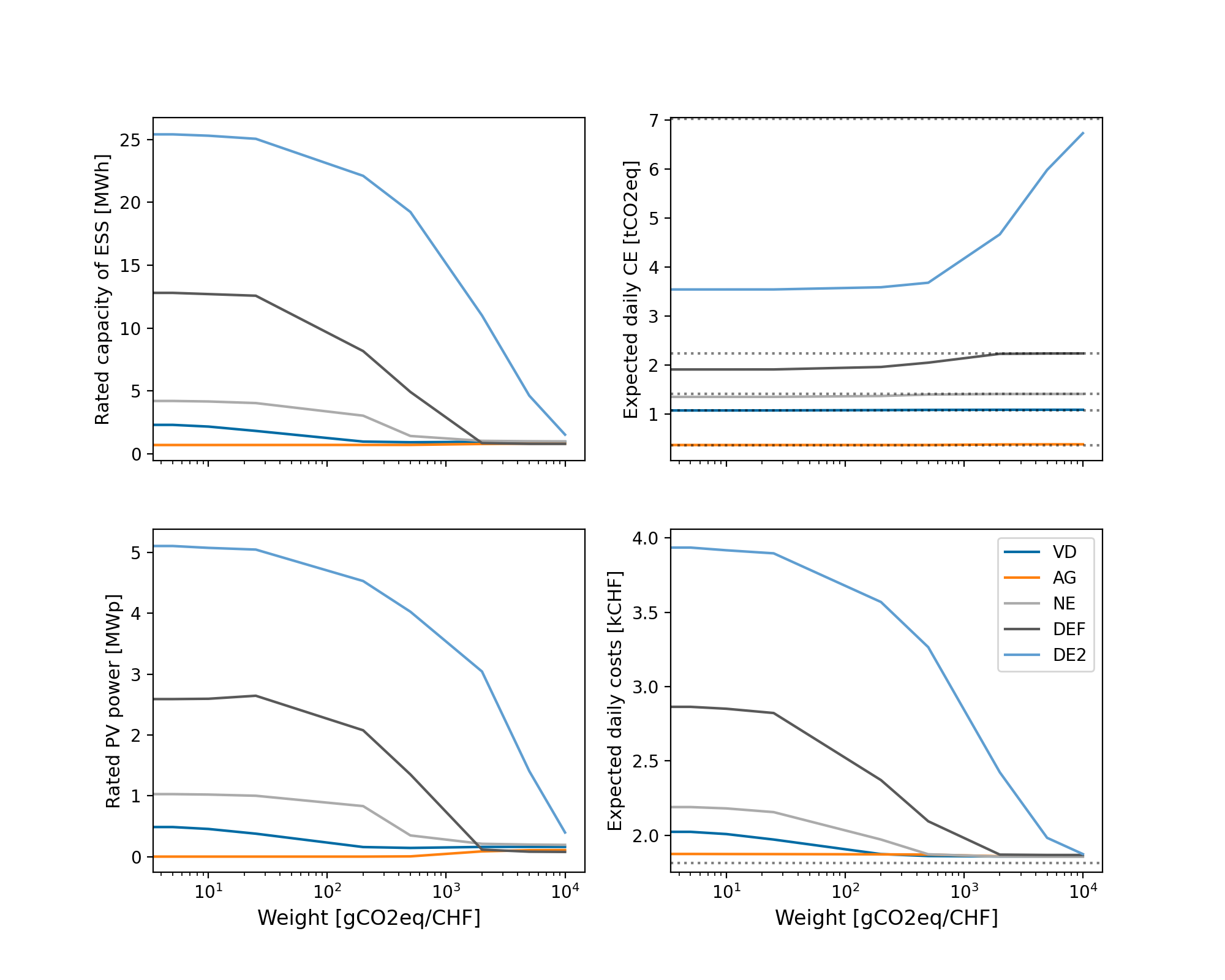
Figure 3: Evolution of decision variables and objectives with increasing $w$, for three Swiss cantons and two NUTS1 regions in Germany.

4.3 Sensitivity to the BESS power to energy ratio

As detailed in Section˜2.3.2, the power to energy ratio of the BESS $r_{\text{ess}}^{\text{p2e}}$ was introduced as an input parameter to convexify the sizing problem formulation. In the results presented above, the parameter is fixed to $r_{\text{ess}}^{\text{p2e}}=1$ (i.e., at 100% state of charge, the battery can provide $P_{\text{ess}}^{\text{rated}}$ for $1\text{\,}\mathrm{h}$), which may not be the optimal ratio for some sizing problems. As discussed in Remark 3, the optimal ratio can be identified by performing multiple sizings with different values of $r_{\text{ess}}^{\text{p2e}}$ and finding the ratio that leads to the smallest value of the objective function. In this section, this process is performed for the case of sizings in canton Neuchâtel and in the Bayern region, with $w=4000$$\text{\,}\mathrm{g}\mathrm{C}\mathrm{O}_{\mathrm{2}}\mathrm{e}\mathrm{q}\mathrm{/}$¤.
Figure 4 shows the evolution of the objectives as the power to energy ratio increases from 0.01 to 1, for canton Neuchâtel on the left and for the Bayern region on the right. The black dotted lines show the baseline expected costs for each objective, while the red dotted lines show the optimal ratios. The top graphs show the evolution of the overall objective, while the middle and bottom graphs show the evolution of the daily cost and footprint respectively. From the top graphs of both regions, $r_{\text{ess}}^{\text{p2e}}=0.25$ and $r_{\text{ess}}^{\text{p2e}}=0.1$ (i.e., as supported by the vertical red dotted lines) can be selected as the optimal ratios for the proposed sizings. Note that the location of the data center impacts the optimal power to energy ratio, as well as the evolution of the sub-objectives (e.g., the middle graphs are evolving in almost opposing ways). Also note that the middle left graph (i.e., the evolution of the operational costs in canton Neuchâtel) shows that a properly sized battery is expected to reduce the expected operational costs of the system compared to the naive selection of $r_{\text{ess}}^{\text{p2e}}=1$.

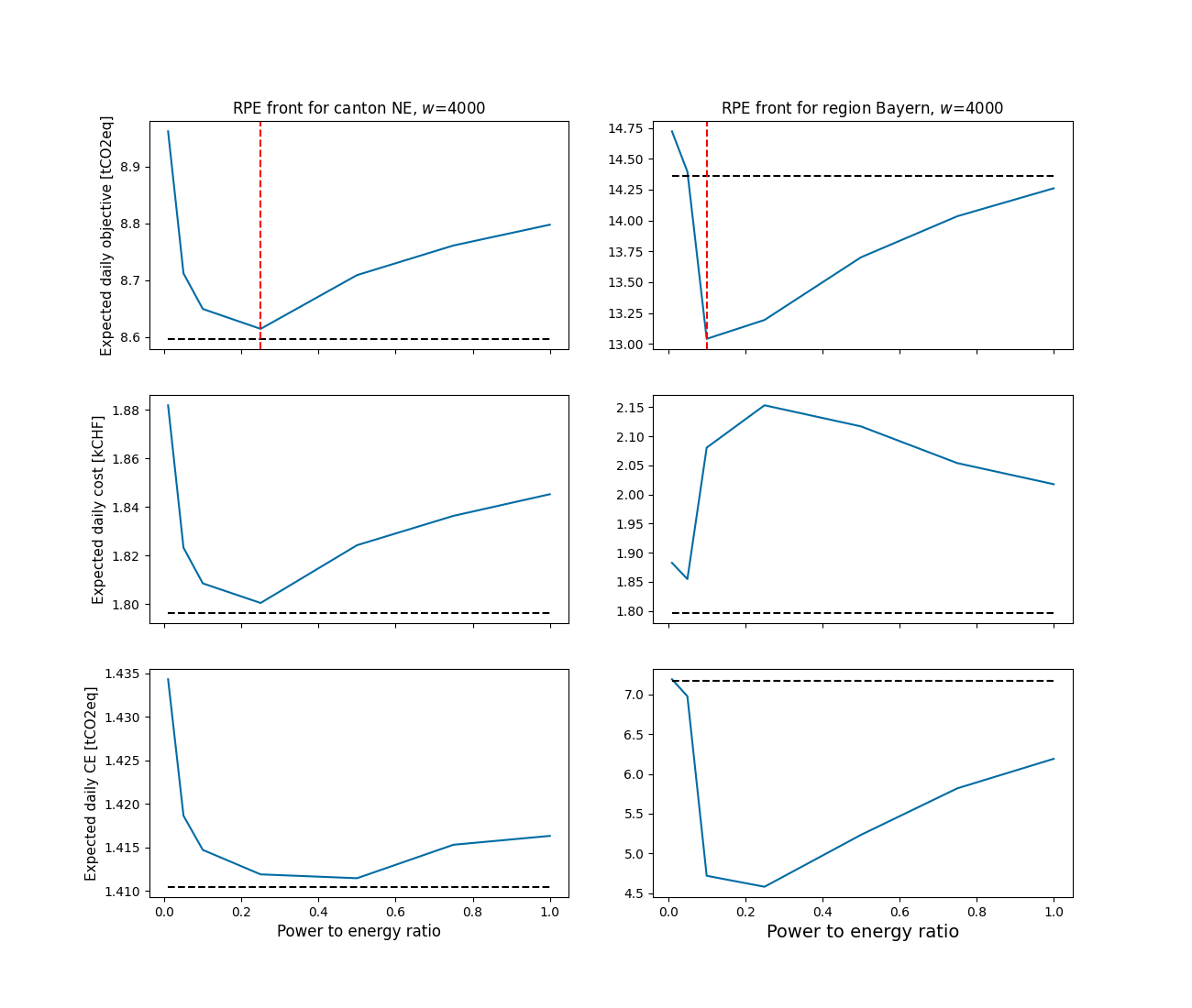
Figure 4: Evolution of objectives with increasing power to energy ratio, for two regions.

4.4 Discussion on the results

The results section used the proposed sizing tool to optimize BESS and PV systems coupled with data centers located in Switzerland and Germany. In Switzerland, while the tool achieves a maximum reduction in carbon emissions of approximately 4%, this comes with a substantial increase in system costs, up to 21%. Although these results show a marginal impact, this is mainly a consequence of the low carbon intensity of the Swiss electricity mix. Indeed, in Germany, the tool achieves maximum carbon reductions of up to 49.6%, though this results in a doubling of operational costs. The analysis highlights that the optimal sizing of BESS and PV systems to achieve data center dispatchability is highly dependent on the data center location. For example, despite the relatively short distance of only $109\text{\,}\mathrm{k}\mathrm{m}$ between the city of Neuchâtel and the city of Aarau, the sizing results for their cantons differ significantly. This demonstrates the necessity to use geographically accurate data when leveraging DER for cost and carbon reduction and the proposed framework can be effectively used to address these location-specific challenges. It is reasonable to suppose that case studies in other countries would lead to different results as, according to [electricitymaps_electricity_nodate] the 2023 yearly average carbon intensity of Switzerland was $86\text{\,}\mathrm{g}\mathrm{C}\mathrm{O}_{\mathrm{2}}\mathrm{e}\mathrm{q}\mathrm{/}\mathrm{k}\mathrm{W}\mathrm{h}$, while it was 4.5 times larger in the United States, Germany, and Ireland (i.e., approximately $400\text{\,}\mathrm{g}\mathrm{C}\mathrm{O}_{\mathrm{2}}\mathrm{e}\mathrm{q}\mathrm{/}\mathrm{k}\mathrm{W}\mathrm{h}$), and 7.7 times larger in India (i.e., approximately $660\text{\,}\mathrm{g}\mathrm{C}\mathrm{O}_{\mathrm{2}}\mathrm{e}\mathrm{q}\mathrm{/}\mathrm{k}\mathrm{W}\mathrm{h}$). Sizing BESS and PV for dispatchable data centers in countries with higher grid carbon intensity (s.a. the U.S., India, etc.) would likely lead to even more opportunities in terms of carbon footprint reduction. Finally, this results section assumes that achieving the dispatchability of the data center complex is an objective of the DCO. It is worth noting that this service does not only benefit the grid (by removing the stochastic behaviour of the power consumption profile), but would likely decrease the intra-day operational costs of the system, as the DCO would not have any imbalance fees to account for.

5 Conclusions

This work proposes a carbon and cost-aware framework to size energy storage systems and photovoltaic generation in the context of a data center aiming at achieving dispatchability, and presents an analysis of the framework in the Swiss and German contexts. The tool can be leveraged by data center operators to easily design a sizing process that takes into account their particular context and needs. Custom grid carbon intensities, DER life cycle assessments, GHI data, load data and custom forecasting methods can be jointly used with the framework. Moreover, user specific inputs provide some flexibility to the users (e.g., the tracking accuracy, the weight $w$, the power to energy ratio, etc.).
The analysis of the method in the Swiss and German contexts highlights the relevance of using geographically granular data in the sizing process, and shows that the method can be successfully used in that perspective. A large difference in the optimal sets of resources is observed: sizings in Bayern suggest BESS capacity ratings up to 36 times larger than sizings in Aargau. Achieving the dispatchability of a data center complex in Bayern is expected to decrease its carbon emissions by approximately 49.6% at best, while, for a DC in Aargau, it is expected to increase its emissions by 2.6% at least. In terms of costs, achieving dispatchability tends to increase the operational costs in all considered regions, although the careful selection of the power to energy ratio of the ESS can reduce the impact on operational costs (e.g. in Neuchâtel and with $w=4000$$\text{\,}\mathrm{g}\mathrm{C}\mathrm{O}_{\mathrm{2}}\mathrm{e}\mathrm{q}\mathrm{/}\mathrm{k}\mathrm{W}\mathrm{h}$, the optimal ratio reduces the operational costs by approximately 3% compared to the naive selection where a unitary ratio is selected).
The main limitation of this work is that the cost of power imbalances are neglected and, therefore, further potential cost savings are not considered. In future work, this limitation will be addressed, as the focus will be shifted towards the day-ahead and intra-day operation of data centers with co-located energy storage and photovoltaic generation, and the economic impact of imbalances will be thoroughly studied.

Author contributions: CRediT

Mario Paolone: Supervision, conceptualization, funding acquisition, resources, validation, visualization, writing - review and editing
Enea Figini: Investigation, methodology, conceptualization, validation, visualization, software, formal analysis, data curation, writing - original draft.

Funding

This work is supported by École polytechnique fédérale de Lausanne, through the Heating Bits Solutions 4 Sustainability project.

Declaration of competing interest

The authors declare that they have no known competing financial interests or personal relationships that could have appeared to influence the work reported in this paper.