A Review on Deep Learning Autoencoder in the Design of Next-Generation Communication Systems

Abstract

Traditional mathematical models used in designing next-generation communication systems often fall short due to inherent simplifications, narrow scope, and computational limitations. In recent years, the incorporation of deep learning (DL) methodologies into communication systems has made significant progress in system design and performance optimisation. Autoencoders (AEs) have become essential, enabling end-to-end learning that allows for the combined optimisation of transmitters and receivers. Consequently, AEs offer a data-driven methodology capable of bridging the gap between theoretical models and real-world complexities. The paper presents a comprehensive survey of the application of AEs within communication systems, with a particular focus on their architectures, associated challenges, and future directions. We examine 120 recent studies across wireless, optical, semantic, and quantum communication fields, categorising them according to transceiver design, channel modelling, digital signal processing, and computational complexity. This paper further examines the challenges encountered in the implementation of AEs, including the need for extensive training data, the risk of overfitting, and the requirement for differentiable channel models. Through data-driven approaches, AEs provide robust solutions for end-to-end system optimisation, surpassing traditional mathematical models confined by simplifying assumptions. This paper also summarises the computational complexity associated with AE-based systems by conducting an in-depth analysis employing the metric of floating-point operations per second (FLOPS). This analysis encompasses the evaluation of matrix multiplications, bias additions, and activation functions. This survey aims to establish a roadmap for future research, emphasising the transformative potential of AEs in the formulation of next-generation communication systems.

I Introduction

In recent years, the field of communication systems has witnessed significant advancements, particularly with the integration of deep learning techniques. Among these, autoencoders (AEs) have emerged as a powerful tool for designing next-generation communication systems, due to their ability to provide end-to-end optimisation systems, i.e., joint optimisation of both the transmitter and receiver. This paper provides a comprehensive survey on the application of AE in communication systems, focussing on their architectures, challenges, and future directions. The primary objective is to explore how AEs can address the limitations of traditional mathematical models, which often rely on simplifying assumptions and may not capture the full complexity of real-world communication environments. Using the data-driven capabilities of AEs, this study aims to identify the enhancement of the system design and performance of communication systems, offering robust solutions using AEs for end-to-end optimisation.

TABLE I: List of Acronyms

Acronym	Full Form	Acronym	Full Form	Acronym	Full Form
ACL	Adjust Carrier Limitation	AE	Autoencoder	AEGNN	Autoencoder Graph Neural Network
AEs	Autoencoders	ADC	Analogue-to-Digital Converters	ADL	Adaptive Deep Learning
AICN	Additive Independent Cauchy Noise	AILN	Additive Independent Laplace Noise	ANNs	Artificial Neural Networks
APQNN	Amplitude Phase Quantization with Neural Networks	AWGN	Additive White Gaussian Noise	BCC	Binary Cross-Entropy
BER	Bit Error Rate	BLER	Block Error Rate	BMD	Bit-Metric Decoding
BNN	Binary Neural Network	BPS	Blind Phase Search	BRNNs	Bidirectional Recurrent Neural Networks
CCE	Categorical Cross-Entropy	CCDF	Complementary Cumulative Distribution Function	CD	Chromatic Dispersion
CE	Cross-Entropy	CGAN	Conditional Generative Adversarial Network	CFAR	Constant False Alarm Rate
CKF	Cubature Kalman Filter	CMA	Constant Modulus Algorithm	CNN	Convolutional Neural Network
CPE	Carrier Phase Estimation	CR	Cognitive Radio	CRNs	Cognitive Radio Networks
CSAE	Channel-Sensitive AE	CSI	Channel State Information	DBN	Deep Belief Network
DL	Deep Learning	DMs	Diffusion Models	DNN	Deep Neural Network
DMs	Diffusion Models	DRdA-CA	Dual-residual Denoising AE with Channel Attention	DSP	Digital Signal Processing
DWDM	Dense Wavelength Division Multiplexing	EKL	Extended Kalman Filter	ELBO	Evidence Lower Bound
ELU	Exponential Linear Unit	FCNN	Fully-connected Neural Network	FMCW	Frequency-modulated Continuous Wave
FLOPS	Floating-Point Operations	FPGAs	Field Programmable Gate Arrays	FSO	Free-Space Optical
GANs	Generative Adversarial Networks	GAs	Genetic Algorithms	GCS	Constellation Shaping
GDR	Generalized Data Representation	GMI	Graphic Mutual Information	GRU	Gated Recurrent Units
IMDD	Intensity Modulation with Direct Detection	ISI	Intersymbol Interference	JSCC	Joint Source-Channel Coding
KLF	Kullback–Leibler	KNL	Kerr Nonlinearity	LPN	Laser Phase Noise
LRV	Latent Random Variables	LSTMs	Long Short-Term Memory	LSTM-AE	Long-Short-Term Memory-Autoencoder
LTE	Long-Term Evolution	LLRs	Log-Likelihood Ratios	M-QAM	M-quadrature Amplitude Modulation
MDC	Multi-Dimensional Constellations	MI	Mutual Information	MIMO	Multiple-Input and Multiple-Output
ML	Maximum Likelihood	MLD	Maximum Likelihood Detection	mmWave	millimeter-Wave
MSE	Mean Squared Error	NC-EA	Noncoherent Energy AE	OFDM	Orthogonal Frequency-Division Multiplexing
OWC	Optical Wireless Communication	PAPR	Peak-to-Average Power Ratio	PCS	Probabilistic Constellation Shaping
PDM	Polarization-Division Multiplexing	PHV	Packet Hot Vector	PN	Phase Noise
PPM	Pulse Position Modulation	PS	Probabilistically-Shaped	QAM	Quadrature Amplitude Modulation
QC-AE	Quantum-Classical Autoencoder	QoS	Quality-of-Service	QNNs	Quantum Neural Networks
QPSK	Quadrature Phase-Shift Keying	RBF	Rayleigh Block Splitting	RF	Radio Frequency
ReLu	Rectified Linear Unit	ResNet	Residual Neural Network	RIS	Reconfigurable Intelligent Surface
RL	Reinforcement Learning	RNNs	Recurrent Neural Networks	RTNs	Radio Transformer Network
SCCE	Sparse Categorical Cross-Entropy	SELU	Scaled Exponential Linear Unit	SER	Symbol Error Rate
SIMO	Single-Input Multiple-Output	SM	Spatial Modulation	SNR	Signal-to-Noise Ratio
SPSA	Simultaneous Perturbation Stochastic Approximation	SSFM	Split-Step Fourier Method	SVD	Singular Value Decomposition
UOC	Underwater Optical Communication	VAEs	Variational AEs	VQ-VAEs	Vector-Quantized Variational AEs
VLC	Visible Light Communication	WC	Wireless Communication	WiFi	Wireless Fidelity

This review comprehensively investigates the application of AE in communication systems, drawing on 120 recent studies published in reputed publishers, including ScienceDirect, Scopus, Springer and IEEE Xplore, including 2024. The literature search used rigorous keywords such as ”Autoencoder in communication system” and ”deep learning in communication system” to identify relevant studies. By categorising these works based on research issues such as transceiver design, channel models, digital signal processing (DSP) techniques, computational complexity, and non-differentiable channels, we provide a structured overview of the current state of the field. Our analysis encompasses various communication domains, including wireless, optical, semantic, and quantum communication, to identify suitable AE approaches for each. Identified AE approaches are analysed based on their architectures, optimisation methods, layer types, activation functions, and loss functions. In addition, several channel models are investigated, including additive white Gaussian noise (AWGN), multiple-input and multiple-output (MIMO), Rayleigh, and optical channels. Note that many existing studies on AE applications in communication systems rely on simplified channel models such as AWGN or basic fibre models. In addition, this review offers in-depth discussions on existing challenges and potential future research directions. To our knowledge, this is the first comprehensive survey of AE applications in communication systems, providing a valuable roadmap for future research.

This reset of this paper is organised as follows. Section II discusses the challenges of designing next-generation communication systems using traditional models and the advantages of employing AEs. Section III elaborates on the advantages and role of AEs in capturing complex relationships and adapting to real-world scenarios. Section IV outlines the practical challenges of implementing AEs, including the need for extensive training data and the risk of overfitting. Section V describes the end-to-end AE learning process, detailing the architecture and training methods. Section VI explores AE-based communication systems, including symbol-wise and bit-wise approaches, various activation functions in AE models, different loss functions used to optimise AE models, the physical constraints that AEs must consider in communication systems, and different variants of AE architecture and their applications. Section VII delves into geometric and probabilistic constellation shaping techniques. Section VIII focusses on differentiable and non-differentiable channels and components, including how to determine differentiability, proposing solutions for non-differentiable scenarios. Section IX details the calculation of the computational complexity of AE. Section X provides a comprehensive review of the literature on the use of AEs in communication systems, covering wireless, optical, semantic, and quantum communication. Section XI suggests future research areas, and finally Section XII concludes the paper by summarising the potential of AEs to revolutionise communication systems.

II Challenges of Designing Next-Generation Communication Systems

Designing next-generation communication systems based solely on mathematical models may prove insufficient due to several reasons (Fig. 1):

• Simplifications and assumptions: Mathematical models often rely on simplifying assumptions or approximations to make complex problems more tractable. These simplifications can lead to inaccuracies if the underlying assumptions are not true in practice. For example, Mathematical models for optical fibre design often start with the assumption that light reflects perfectly within the fibre due to total internal reflection, with no losses at the boundaries. Thus, incorporating realistic factors such as scattering, surface roughness, and connector losses into the models is crucial to ensure accurate design and reliable operation [1].

• Limited scope: Mathematical models may be developed for specific scenarios or conditions by focusing on a specific aspect of the system, such as signal propagation or noise analysis. But they fail to capture the full range of possible operating environments or use cases. For example, when designing optical fibres, ideal properties like uniform refractive index profiles and perfectly circular cores is normally assumed. However, real-world fibres have imperfections due to manufacturing processes, impurities, and microbending losses. These imperfections affect signal propagation, dispersion, and attenuation. Mathematical models may overlook these [2, 3, 4]. On the other hand, as wireless networks increasingly adopt millimeter-wave (mmWave) frequencies, these limitations in scope become more pronounced. Modelling the interaction of signals with environmental factors such as walls, buildings, and even human bodies is crucial for 5G and future systems [5].

• Lack of physical insight: Over-reliance on mathematical models can lead to a lack of understanding of the underlying physics and mechanisms. This can make it challenging to optimise performance when unexpected behaviour arise [6]. In wireless communication systems, understanding the physical mechanisms behind phenomena such as small-scale fading is critical, particularly in high-mobility scenarios like vehicular networks where doppler shifts play a significant role [7]. In optical communication system, by designing a dense wavelength division multiplexing (DWDM) optical communication system, over-reliance on linear mathematical models can overlook nonlinear effects like four-wave mixing, self-phase modulation, and scattering, leading to unanticipated crosstalk, spectral broadening, and power loss [8]. This lack of physical insight complicates troubleshooting and optimisation, as engineers may struggle to diagnose and mitigate issues like increased BER and reduced transmission distance. Combining models with a deep understanding of the underlying physics is crucial for effective design and maintenance.

• Inadequate representation of complexity: In wireless communication where a system is operating in environments with high mobility, like long-term evolution (LTE) and 5G networks, it normally can face complex interactions due to handovers, interference, and dynamic spectrum allocation. For example, traditional models may inadequately capture fast-fading environments or the effects of interference in dense deployments of small cells, leading to inaccurate predictions of quality-of-service (QoS) [9]. In optical fibre communication, a system involves complex interactions between light, matter, and energy. Mathematical models may struggle to accurately represent these complexities, leading to inaccuracies in predictions or simulations. For example, mathematical models might inadequately represent the combined impact of chromatic dispersion (CD) and nonlinearities like four-wave mixing, leading to inaccurate predictions of signal degradation over long distances. This simplification can result in underestimating the need for dispersion compensation or additional amplification, ultimately causing performance issues and increased BER in practical deployments [10].

• Validation challenges: Verifying wireless communication models is particularly challenging in environments with high variability, such as urban or suburban landscapes. For example, testing models for 5G small-cell deployments in different topographies and with varying levels of interference requires extensive field trials or real-world comparisons that are often difficult to scale [11]. In optical fibre communication systems, verifying the accuracy of mathematical models is difficult due to their complexity. Therefore, validation may require extensive experimental testing or comparisons with other models [3, 4, 12].

• Inadequate consideration of uncertainties: Mathematical models typically assume deterministic behaviour, neglecting the inherent uncertainties and noise present in real-world systems. This can lead to overly optimistic predictions or simulations that do not accurately reflect actual system performance. For example, wireless systems are often subject to signal fading, interference, and fluctuating traffic patterns. Mathematical models for wireless communication may oversimplify by assuming independent, identically distributed channels, whereas in real scenarios, channels are often correlated due to shadowing or mobility [13].

• Complexity and nonlinearity: Communication systems often exhibit nonlinear behaviour, which can be challenging to model using traditional mathematical techniques due to the difficulty in capturing nonlinear effects. Wireless communication systems, where multi-antenna configurations like massive MIMO are involved, exhibit nonlinear behaviour that can be difficult to model. Interference among multiple users, nonlinearities in radio frequency (RF) components, and beamforming algorithms all introduce complex interactions that challenge traditional linear models [14]. An example in fibre optical communication is a DWDM system with multiple channels where the nonlinear effects (such as self-phase modulation and cross-phase modulation) become significant as the signal power increases. These effects lead to inter-channel crosstalk and impairments that cannot be accurately predicted by simple mathematical models [3, 4, 15]. To account for these nonlinearities, advanced numerical simulations or experimental measurements are necessary .

• Lack of integration with other disciplines: Mathematical models may not effectively integrate knowledge and insights from related fields such as electrical engineering, materials science, or physics [16]. In wireless communication, it often requires interdisciplinary approaches to combine elements of materials science, such as antenna design, and RF circuit design. Specifically, advances in metamaterials could influence how antennas are modelled, but traditional mathematical approaches might not fully integrate these insights, leading to a gap between theory and practice [17].

Figure 1: Communication System Mathematical Model Limitation

Although mathematical models provide valuable information, next-generation communication systems require a holistic approach that considers the above limitations. One promising solution is end-to-end deep learning using AE, which can bridge the gap between mathematical models and real-world complexities, contributing to robust communication systems.

III Why AEs and their Role

An end-to-end learning using AE provides a data-driven approach that complements mathematical models. By capturing intricate relationships and adapting to the complexities of the real world, AEs contribute to the development of robust communication systems. The primary advantages of employing AEs in communication systems include the following.

• Minimising Distortion: The basic idea behind an AE is to transfer input to output with the least possible distortion, which is perfectly in line with the purpose of a communication system.

• Framework Alignment: AEs precisely follow the communication system framework, where the encoder acts as the transmitter and the decoder acts as the receiver.

• Expressive Latent Representation: AEs can create expressive latent representations for complex data, which can be adapted to suit the physical conditions of the communication system.

• Flexibility: The AE Architectures offer flexibility to be modified for various tasks within communication systems, enhancing their adaptability and efficiency.

Therefore, an end-to-end learning based on AE is an elegant candidate to address the challenges in next-generation communication systems such as:

• AEs can learn nonlinear mappings between input ( received optical signals) and latent representations. Training an AE on real-world data can capture the complex nonlinearities present in the system. For example, an end-to-end AE can model the nonlinear effects in DWDM systems, such as interchannel crosstalk due to self-phase modulation.

• AEs can learn compact representations of input data. By encoding and decoding signals, they capture essential features while ignoring noise or imperfections. For example, in fibre design, an AE can learn to represent the refractive index profile of the fibre. It accounts for imperfections (non-uniformity) and helps optimise fibre parameters while considering physical limitations.

• AEs adapt to changing input distributions. They can learn from historical data and generalise to new conditions. For example, an AE trained on diverse temperature profiles can predict signal behaviour in a temperature-varying fibre link. It can adapt its latent representation to dynamic environments.

IV Challenges of using AE in practical scenarios

Generally the use of AE in practical scenarios can be divided into online and off-line approaches. The off-line approach is that the encoder and decoder parts of the AE model are trained offline based on a real-world dataset. Once training is complete, both can operate independently on the transmitter and receiver sides of the respective communication system. The online approach is that the AE model has partially, or maybe completely, replaced the transmitter and receiver parts of the communication system. This AE model can be pre-trained based on real data-set. There are several challenges when it comes to using AEs in practical scenarios.

• AE learning from end-to-end needs a significant amount of training data to be effective.

• AEs can sometimes overfit the training data, which can lead to poor performance with new unseen data. To solve this, a regularisation technique can help prevent overfitting and improve the robustness of the model to noisy data. A powerful technique is to equip each layer with batch normalisation. This normalisation significantly accelerates training and effectively mitigates overfitting [18, 19].

• AE model may not perform as well in real-world scenarios as it does in the training environment because the AE model may not be able to deal with the unexpected noise or confidence in the input data and practical. There are several methods that can be used to deal with unexpected noisy or corrupted data in practical applications. One approach is to pre-process the data before feeding them into the model, such as cleaning them or removing any obvious outliers. Another option is to use data augmentation techniques, which involve generating multiple variants of the data to increase the amount of training data available to the model. This can help the model learn to handle different types of noise and inconsistencies in the data.

• An online end-to-end AE learning requires a differentiable channel model to train the transmitter, that is, transmitter training necessitates backpropagating the gradient through the channel. Section VIII-B provides detailed information on potential solutions.

V End-to-end AE Learning

An end-to-end AE is a deep neural network (DNN) model that learns representations (encoding) for sets of data by attempting to reproduce its input in the output. It is an unsupervised machine learning algorithm. This means that it does not require labelled output or targets during training and instead tries to reconstruct inputs from their encoded representation in hidden layers. As shown in Fig. 2, the architecture can be divided into three main parts: Encoder (mapping input $x$ to latent space $w$), Latent Space $w$ (bottleneck), and Decoder (mapping latent space $w$ to output $\hat{x}$).

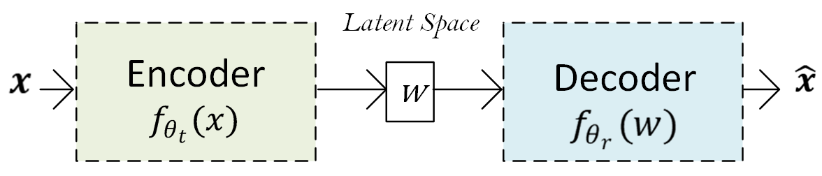
Figure 2: AE Architecture

1. Encoder: The encoder part of the AE takes input data, which can be any form of structured data, and is typically composed of a series of neural network layers with nonlinear activation functions such as rectified linear unit (ReLu) or exponential linear unit (ELU). Its goal is to transform the high-dimensional input into a lower-dimension latent space representation that captures the most important features in an efficient manner.

2. Bottleneck/Latent Space: This part of AE represents compressed knowledge about the original data and is typically composed of one or more un-trainable layers with fewer neurons than the input layer, hence creating a bottleneck effect where only important features are kept while less significant ones get discarded.

3. Decoder: The decoder part of an AE takes the compressed representation and reconstructs the original data from it. It mirrors the encoder architecture but in reverse, attempting to output a reconstruction that is as close as possible to its input (though not necessarily identical due to noise or other factors).

The entire process can be summarised as follows. Input $\mapsto$ Encoding $\mapsto$ Bottleneck/Latent Space $\mapsto$ Decoding $\mapsto$ Output. The AE learns optimal weights during training, which minimises the reconstruction error between inputs and outputs using a loss function. The key advantage of an end-to-end learning approach is that it allows for more efficient data preprocessing or feature extraction since all these tasks are learned simultaneously. It also helps to capture complex patterns within the input data, which can be useful when dealing with high-dimensional datasets.

VI AE based Communication systems

Traditional communication systems employ a block-based approach, where separate transmitter and receiver signal processing blocks are cascaded as shown in Fig. 3 (a). This approach often leads to suboptimal performance due to two main challenges: (1) the difficulty of accurately modelling complex physical channels, as discussed in Section II, and (2) the need to develop specific algorithms to compensate for these effects based on the chosen mathematical model. A promising solution is to use DL-based approaches, inspired by AE architectures [20]. As shown in Fig. 3 (b), by taking advantage of the ability of deep learning models to learn robust latent representations, AE-based systems have the potential to optimise end-to-end communication performance. The latent space representation produced by the encoder is passed through a channel model, where it undergoes channel impairments and produces $y$. Thus, instead of relying on a chain of separate transmitter and receiver signal processing blocks, a data-driven model based on AEs architecture can effectively capture the characteristics of the communication channel, enabling more efficient and reliable transmission.

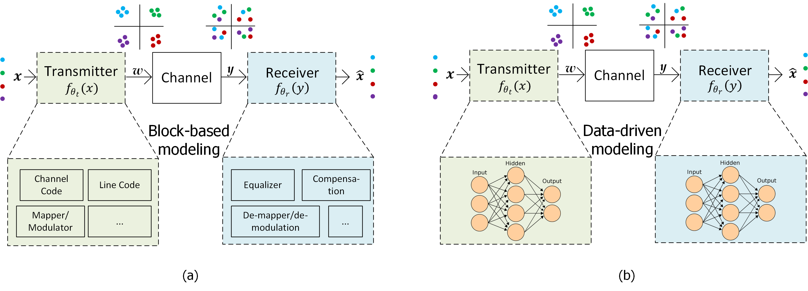
Figure 3: Communication System (a) Classical Block-based Model (b) AE Data-driven Model

The main goal of a communication system, acting as an AE, is to find a robust latent space representation $w$ of the input data in the transmitter to counteract any impairments introduced by the channel. In particular, through an end-to-end training, the AE learns to effectively reconstruct the input data at the receiver, considering the presence of channel impairments. During the training process, the encoder component of the AE acquires resilient symbol sequence representations for all incoming data. Once training is complete, both the transmitter and the receiver can function independently, using their respective layer dimensions and weights. The remainder of this section delves into the various aspects of employing AEs in communication systems, encompassing the two AE approaches, activation functions, loss functions, physical constraints, and AE architectural variants.

VI-A Symbol-Wise and Bit-Wise AE

Symbol-wise AEs and Bit-Wise AEs are two different approaches to designing a communication system. Their primary difference lies in how they handle the mapping of symbols or bits from input messages to effectively determine the learnt constellation. This may directly impact system performance characteristics such as bit error rate (BER), symbol error rate (SER), and computational complexity. The learnt constellations of a symbol-wise AE model do not account for a bit-labelling scheme. Therefore, determining the optimal labelling scheme for the learnt constellations is a key challenge. To address this, a bit-wise AE approach offers a more direct optimisation path. To optimise geometric constellation shaping (GCS), symbol-wise AE can be trained for that, while bit-wise AE can be trained jointly for GCS and bit labelling [21]. In both symbol-wise AE and bit-wise AE, the input to the encoder AE can be pre-processed to one hot encoded.

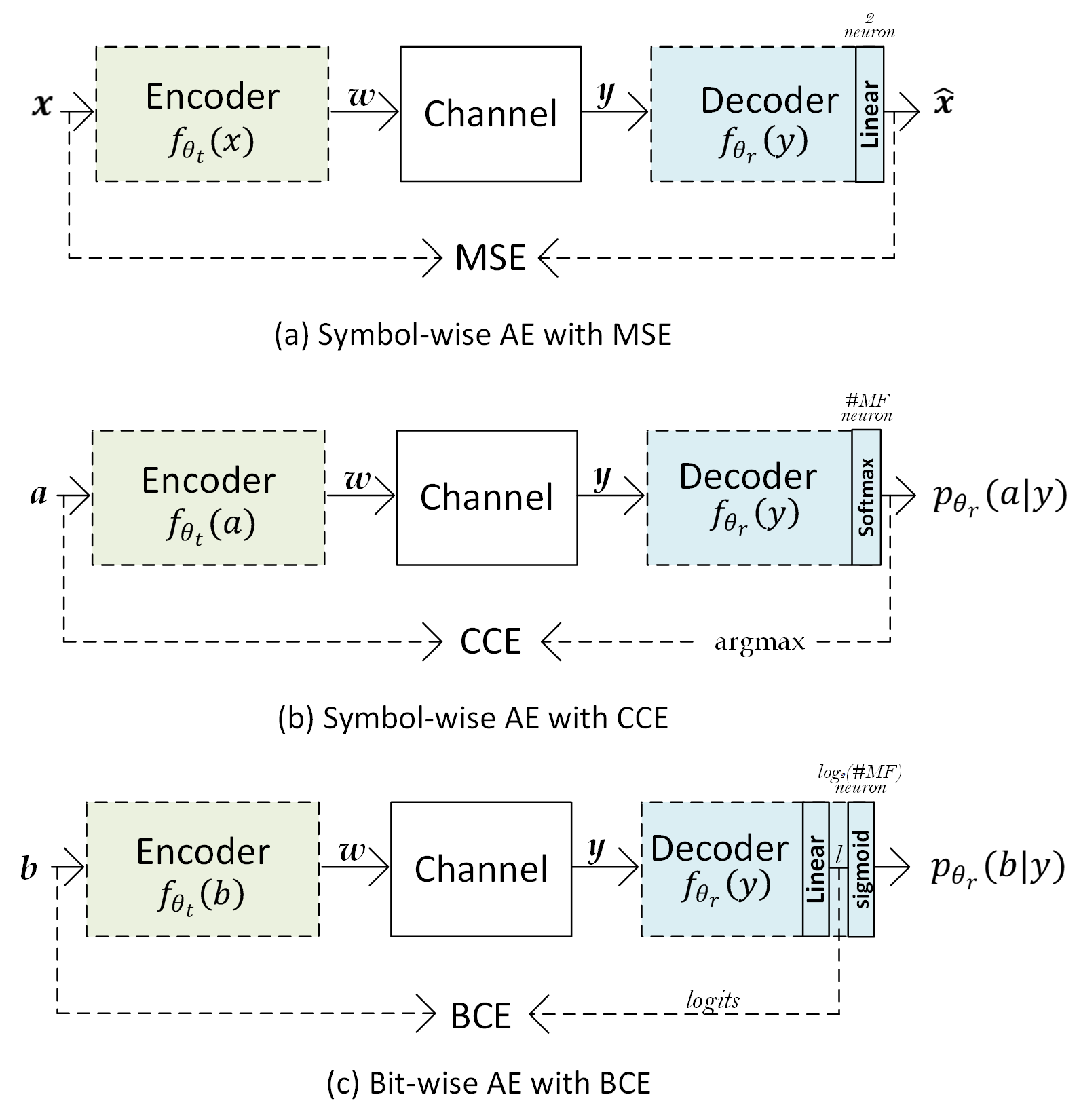
Figure 4: Symbol and Bit-wise AE learning based communication system

Fig. 4 shows three different end-to-end learning architectures based on AE. Regression problems can be used in AEs for end-to-end learning of communication systems. By setting the output layer of the AE to a linear regression layer as shown in Fig. 4 (a), the AE can be trained to predict continuous values for new inputs[22, 23]. This results in complex output data consisting of both in-phase (I) and quadrature (Q) components. This data is then fed into a demapper for symbol detection and subsequently a hard decision circuit to recover the original bit sequence. The AE encoder processes complex baseband symbols ($x\in\mathbb{C}$) from modulation formats such as quadrature phase-shift keying (QPSK), or M-quadrature amplitude modulation ($M$-QAM). The encoder, parametrised by $\theta_{t}$, generates resilient latent representations ($w\in\mathbb{C}$) by mapping $f_{\theta_{t}}:x\mapsto w$. These representations are then passed through a channel model, where they undergo impairments. The decoder, parameterized by $\theta_{r}$, aims to reconstruct the original symbol from the channel-corrupted output ($y\in\mathbb{C}$) by mapping $f_{\theta_{r}}:y\mapsto\hat{x}$, where $\hat{x}\in\mathbb{C}$. As it tries to predict the data of a numerical symbol, the Mean Squared Error (MSE) is a suitable loss function; see Section VI-C. Since NNs cannot directly process complex data, the $N$ complex input data must be converted to $2N$ real-valued representation for both the encoder and decoder by implementing a $\mathbb{C}2\mathbb{R}$ layer. The resulting real-valued output is then converted back to complex data by using a $\mathbb{R}2\mathbb{C}$ layer.

Alternatively, as shown in Fig. 4 (b), a symbol-wise approach based on minimising categorical cross-entropy (CCE) can be fed with a message $a\in\{0,1,...,M-1\}$, $M$ denotes the number of different symbols as $M=2^{m}$ where $m$ is the number of bits per symbol. Thus, the encoder then processes the mapping to complex data as $f_{\theta_{t}}:\{0,1,...,M-1\}\mapsto w$, i.e. $f_{\theta_{t}}:a\mapsto w$. Another key distinction lies in the output layer, the Softmax activation layer, which is used to obtain a probability vector of length $M$ which corresponds to the probabilities of possible $M$ messages, $p_{\theta_{r}}(a|y)$ [21]. This represents the estimated posterior distribution of the transmitted signal given the received signal. The constellation obtained through symbol-wise training is not optimised for bit-labelled. Bit-labelled indicates that each constellation point must be uniquely mapped to a specific bit vector. To enable joint constellation optimisation and bit labelling, a bit-wise AE can be used, as shown in Fig. 4 (c), can be used. $m$ length input bit vector $m$ length $m$ length $m$ length $b$ can be fed to the encoder to perform the mapping $f_{\theta_{t}}:b\mapsto w$. The AE output is used directly without applying an activation function. These output values are called logits ($l$) which is a raw data and represents un-normalised probabilities of the data belonging to a specific class. Logits are normally suitable for classification tasks. Therefore, the loss function of BCE is suitable for such an approach. The Sigmoid function outputs a probability for each bit independently, which is applied to the decoder logits $l$ . This allows for the direct computation of the estimated posterior probabilities $p_{\theta_{r}}(b|y)$ for each bit, facilitating the use of log-likelihood ratios (LLRs) in the analysis [21]. The minimisation binary cross-entropy (BCC) function can then be used to optimise the AE, more details are given in Section VI-C.

VI-B Activation Functions

In the context of using AE for end-to-end learning in communication systems, a list of possible activation functions can be seen in Table II. The ReLU is widely used in hidden layers of encoder and decoder parts of the AE model. The ELU activation function is a non-saturating function that accelerates training while mitigating the risk of gradient explosion or vanishing gradient problems. The existing literature commonly employs ReLU and/or ELU activation functions in the hidden layer of AE-based communication systems. For example, [24] initially employed ReLU in their AE model but later switched to ELU in [25] for improved results. Therefore, it is highly recommended to investigate both in order to determine the optimal choice. Additionally, further research is needed to determine the combination use of both in the AE model, for example, one for the encoder and the other for the decoder. However, the LeakyReLU activation function allows for a small, non-zero gradient when the input is negative, which helps mitigate the ”dying ReLU” problem often encountered with standard ReLU activations. This ensures a small gradient when the unit is inactive, which helps to keep the learning process alive [26]. Tanh activation has zero-centred output, which can make optimisation easier. It is also useful in hidden layers to model complex relationships. In [27], Tanh activation is used to extract the feature. In [28], it is used in all the 1D convolutional layers. The scaled exponential linear unit (SELU) can induce self-normalisation, which means that the activation automatically converges to zero mean and unit variance, as can be seen in Table II where $\lambda\approx 1.0507$ and $\alpha\approx 1.6733$. This helps maintain the stability of the model during training, which is crucial for AEs that require consistent encoding and decoding [29]. It is suited for the hidden layer of AEs to leverage its self-normalisation, which can lead to faster convergence. More research is required to investigate the potential benefits of alternative activation functions, such as Swish, for better gradient flow in the hidden layers. Finally, Softmax and Sigmoid activation layers are typically used in the output layer for classification tasks. The first can be used for symbol detection, while the second can be used for binary detection.

TABLE II: Common Activation Functions in AE-based communications

Name	Function	Output Range
ReLU	$\text{ReLU}(x)=\max(0,x)$	[0, $\infty$)
ELU	$\text{ELU}(x)=\begin{cases}x&\text{if }x\geq 0\\ \alpha(e^{x}-1)&\text{if }x<0\end{cases}$	($-\alpha$, $\infty$)
Leaky ReLU	$\text{Leaky ReLU}(x)=\begin{cases}x&\text{if }x\geq 0\\ \alpha x&\text{if }x<0\end{cases}$	($-\infty$, $\infty$)
Tanh	$\tanh(x)=\frac{e^{x}-e^{-x}}{e^{x}+e^{-x}}$	($-$1, 1)
SELU	$SELU(x)=\begin{cases}\lambda x&\text{if }x>0\\ \lambda\alpha(e^{x}-1)&\text{if }x\leq 0\end{cases}$	[$-$1.758, $\infty$)
Swish	$\text{Swish}(x)=x\cdot\sigma(x)$	($-\infty$, $\infty$)
Softmax	$\text{Softmax}(x_{i})=\frac{e^{x_{i}}}{\sum_{j}e^{x_{j}}}$	(0, 1)
Sigmoid	$\sigma(x)=\frac{1}{1+e^{-x}}$	(0, 1)

VI-C Loss Functions

In the context of communication systems, there are two variant ways of dealing with the communication problem, either as a regression problem or a categorical problem [30]. A regression problem in the context of machine learning and communication systems typically involves predicting continuous or numerical data based on the input data. By setting the output layer of the AE to a regression layer (such as a linear layer), the AE can be trained to reconstruct a continuous target value, which can be used effectively in communication systems.

In contrast, in classification problems, the predicting data is a categorical or discrete class. End-to-end AE learning for communication systems using a classification problem involves training the AE to recognise and classify different constellation diagrams such as QPSK, 16-QAM, and 64-QAM, based on the structure and shape of the diagrams. This can be done by setting the output layer of the AE to a classification layer (such as the sigmod activation layer) and compute the cross-entropy. This way can be useful in applications such as the evaluation of symbol error rate and the evaluation of communication system performance.

VI-C1 Mean Squared Error (MSE)

It serves as a loss function during the training phase, which is determined by computing the mean squared deviations between the predicted values and the actual ground truth values [31]. The general expression of the MSE is

$$\mathcal{L}_{MSE}=\frac{1}{N}\sum^{N}_{i=1}|X_{estimate}-X_{true}|^{2},$$ (1)

where $N$ is the number of samples, $X_{estimate}$ and $X_{true}$ are the estimate and ground-truth values. As AE consists of two parts: an encoder and decoder, the encoder mapping can be expressed as $w=f(x;\theta_{t})$, which produces the latent representation $w$ (see Fig. 4(a)). The decoder mapping, on the other hand, can be expressed as $\tilde{x}=f(y;\theta_{r})$, which reproduces a replica of the original input values of $x$. The $\theta_{t}$ and $\theta_{r}$ are the training parameters of the encoder and decoder parts, respectively. The channel layer of the AE architecture is differentiable but not learnable. As a consequence, the MSE of the proposed AE is defined as

$$\mathcal{L}_{MSE}(\theta)=\frac{1}{N}\sum^{N}_{i=1}|f(x;\theta)-x|^{2},$$ (2)

where $\theta=\{\theta_{t},\theta_{r}\}$ are the learning parameters of the AE model.

Gradient-based learning [32, 33] is employed to find optimal parameters $\theta=\{\theta_{t},\theta_{r}\}$ that minimize the loss function $\mathcal{L}_{MSE}(\theta)$ as

$$\theta=\text{argmin}(\mathcal{L}_{MSE}(D_{set};\theta)),$$ (3)

where $\mathcal{L}_{MSE}(D_{set};\theta)$ is the loss associated with $D_{set}$ set of data. This is achieved iteratively by updating $\theta$ using gradient descent as

$$\theta_{i}=\theta_{i-1}-\beta\Delta\mathcal{L}_{MSE}(D_{set};\theta_{i-1}),$$ (4)

where $\beta$ represents the learning rate, and the Stochastic Gradient Descent, such as Adam optimiser, enhances convergence.

VI-C2 Cross-Entropy (CE)

CE is a widely used metric for training classification models since it is differentiable, which is crucial for gradient-based optimisation algorithms[34, 35]. It is a quantitative metric in information theory that is used to measure the divergence between two probability distributions. This means that it measures the dissimilarity between two probability distributions. In the context of neural networks, one distribution is the output of the predicted probability distribution by the network, and the other is the true (target) distribution. Categorical cross-entropy (CCE) and sparse categorical cross-entropy (SCCE) are two additional variations of the Cross-Entropy. While both are used for multiclass classification, the latter is optimised for datasets with integer encoded labels, offering computational efficiency benefits. One challenge of using CE is that it can be sensitive to class imbalance, where one class has significantly more samples than the other. This can lead to biased models.

Given a predicted probability distribution $p$ and a true distribution $q$, the cross-entropy is defined as:

$$H_{CE}(p,q)=-\sum_{i}q_{i}log(p_{i}),$$ (5)

where $i$ iterates over all possible classes, $p_{i}$ is the learned probability of class $i$, and $q_{i}$ is the true posterior distribution of class $i$.In the context of AE end-to-end learning, the learned probability distribution is defined $p_{\theta_{r}}(a|y)$ as shown in Fig. 4 (b). The encoder with the learning parameter $\theta_{t}$ is trained to output the symbol distribution $f_{\theta_{t}}(a)$ based on the input data $a$. The optimisation of the AE model is then promised by minimising CCE [36] as

$$H_{CCE}(p,q)=-\sum_{a,y}p_{\theta_{t}}(a|y)log(p_{\theta_{r}}(a|y)).$$ (6)

In the case of binary classification, where $q$ is a one-hot vector, the equation simplifies to:

$$H_{BCE}(p,q)=-zlog(p)-(1-z)log(1-p),$$ (7)

where $z$ is the true label (0 or 1), and $p$ is the predicted probability of the positive class. This is known as BCE [37].

TABLE III: Loss Functions Comparison

Loss Function	Advantages	Disadvantages	Use Cases
MSE	• Intuitive: measures the average squared difference between predicted and true values. • Widely used in regression tasks.	• Sensitive to outliers: outliers can have a significant impact on the loss. • Less suitable for classification tasks: may not be as informative for classification problems.	Regression tasks
BCE	• Interpretable: Directly measures dissimilarity between predicted and true distributions. • Differentiable: suitable for gradient-based optimisation. • Efficient: can be computed efficiently. • Widely used: standard loss function in many ML frameworks.	Sensitive to class imbalance and assumes independence of classes	Binary classification tasks
CCE	Same as BCE	Same as BCE	Multi-class classification tasks
SCCE	More efficient for large datasets with integer-encoded labels	Same as binary CE	Multi-class classification tasks with integer-encoded labels

VI-D Physical constraints

AEs offer significant value due to their ability to learn latent representations under various constraints. By tailoring the training process, AEs can be designed to capture specific desired properties within the latent space. In the context of communication systems, this enables generating a signal that acknowledges physical limitations. Therefore, some constraints can be introduced to generate robust signal based on specific physical limitations, such as:

• Average power, energy, amplitude constraints,

• Bandwidth constraint,

• Peak-to-average power ratio (PAPR) constraint, and

• Adjust carrier limitation (ACL) constraint.

The constraints can be realised in several ways. One way is to incorporate a regularisation layer into the trainable network, within the AE encoder part. This layer can effectively maintain the level of encoded signals by amplitude $|w_{i}|\leq 1\ \forall w_{i}$, average power $\mathop{\mathbb{E}}[|w_{i}|^{2}]\leq 1\ \forall w_{i}$, or energy $||w||_{2}^{2}\leq n$, where $n$ is channel use [38, 39]. Some constraints such as reducing PAPR and ACL can be overcome by introducing an additional loss function that penalises the AE encoder to promote a restriction on the transmit signal such as [40].

$$\mathcal{L}_{total}=\alpha_{AE}\mathcal{L}_{AE}+\alpha_{add}\mathcal{L}_{add},$$ (8)

where $\mathcal{L}_{AE}$ is the AE loss function like MSE or CE, and $\mathcal{L}_{add}$ is the added penalties to realize the constraints. $\alpha_{AE}$ and $\alpha_{add}$ are the weights in penalties that help determine how much importance is given to minimising the loss of the learning process. This penalty is applied exclusively to the encoder weights[24, 25, 41].

VI-E AE Architecture Variant

Based on the existing literature, the following AE architectures have been used in communication systems:

VI-E1 Classical AEs

They typically use fully connected layers (also known as dense layers) [19]. This is the simplest form of an AE and is designed for general-purpose dimensionality reduction or feature learning tasks. In this architecture, both the encoder and the decoder are composed of fully connected layers, where each neurone in a layer is connected to every neurone in the subsequent layer. This means that the AE maps the input directly to a lower-dimensional latent space and back to the original space.

VI-E2 Convolutional AEs

They are based on convolutional neural network (CNN), the convolutional AEs utilise convolutional layers instead of fully connected layers. This architecture is more suitable for handling large, high-dimensional data by efficiently learning spatial patterns. Several CNN architectures have been proposed, such as AlexNet, ZefNet, ResNet, etc., more details are available under [19].

VI-E3 Recurrent AEs

These RAEs use recurrent neural networks (RNNs), such as long short-term memory (LSTMs) or gated recurrent units (GRUs), to handle sequential data. The main idea is to leverage the sequential processing capabilities of RNNs to reconstruct ordered or temporal data the same way traditional AE work with static data [42].

VI-E4 Variational AEs

They are a generative model that learns the input data distribution and can generate new data samples [42]. Unlike classical AEs that learn a deterministic mapping from input to latent space, variational AEs (VAEs) learn a probabilistic latent space. This makes them more robust for generating realistic and diverse outputs. The encoder in VAEs outputs two vectors: the mean $\mu$ and the standard deviation $\sigma$ of a latent variable distribution. Instead of encoding the input to a fixed latent vector, VAEs assume that the latent space follows a Gaussian distribution. In addition to the reconstruction loss function that measures how well the reconstructed data match the input, the Kullback-Leibler (KL) divergence loss is used to measure how close the learnt latent distribution is to the standard Gaussian distribution:

VI-E5 Sparse AEs

These SAEs impose sparsity constraints on hidden layers, ensuring that only a few neurones are activated at a time. This forces the AE to learn efficient and compact representations of the input data, even if the dimensionality of the latent space is not explicitly reduced. they are typically enforced by adding a regularisation term such as penalty to the loss function. This encourages the network to activate only a subset of neurones.

VI-E6 Adversarial AEs

These AAEs utilise generative adversarial networks (GANs) to regularise the learnt latent space, making it match a specific prior distribution [42]. The goal is to achieve better generative capabilities, producing more realistic and diverse data compared to traditional AEs. Along with the reconstruction loss function, adversarial loss is used to ensure that latent space follows a target prior distribution. Compared to VAEs which use a probabilistic approach with KL divergence, AEs use adversarial training through a GAN framework.

Future research should investigate in more depth the following AE architectures for the area of communication systems [42]:

• Bayesian AEs

• Diffusion AEs

• Contractive AEs

• Denoising AEs

• Semi‑supervised AEs

• Masked AEs

VII Geometric and Probabilistic Constellation Shaping

Geometric and probabilistic constellation shaping are two techniques used to optimise the performance of communication systems [43, 44, 45, 46, 47]. Although they share some similarities, there are also significant differences between them. Table IV presents the main differences between them.

GCS aims to optimise the constellation shape for better performance by optimising the spatial distribution of modulation symbols in a two-dimensional plane. That is, it involves designing a specific geometric shape for the modulation format to achieve better performance in terms of maximising the signal-to-noise ratio (SNR) or minimising the BER. This is typically done by defining a set of rules or constraints that define the geometry of the constellation and then optimising the modulation format accordingly. GCS can be achieved through various methods, such as mathematical optimisation techniques, graph theory-based approaches, or machine learning algorithms.

On the other hand, probabilistic constellation shaping (PCS) involves controlling the probability distribution of constellation points. That is, it considers the geometric distribution and introduces a probabilistic aspect to it. Control both symbol distance and their occurrence probabilities in order to optimise system performance further. The aim is typically two-fold: to enhance spectral efficiency while simultaneously improving the SNR for better BER. This is typically done by optimising the modulation format to achieve better performance in terms of data rate, reach, and noise tolerance. Probabilistic shaping can be achieved through various methods such as optimisation algorithms, machine learning techniques, or signal processing approaches.

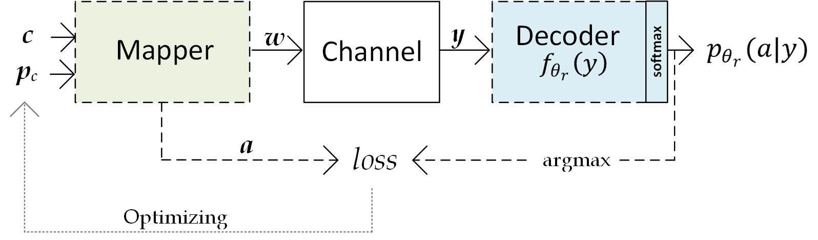
Figure 5: Geometric ($c$) and probabilistic ($p_{c}$) constellation shaping

Another key difference is the level of complexity involved in each approach. GCS can be simpler to implement, but may have limitations in terms of flexibility and adaptability to changing channel conditions. On the other hand, PCS can be more complex to implement and optimise due to its dual consideration - optimising both spatial and temporal aspects (occurrence probabilities), and it requires advanced mathematical techniques and signal processing algorithms. In the context of end-to-end learning based on AE in the communication system, joint geometric and probabilistic shaping can optimise the constellation for enhanced performance, such as maximisation of mutual information [48, 49, 50]. Fig 5 illustrates the two inputs to the mapper on the transmitter sides: the constellation points $c$ and their corresponding probabilities $p_{c}$. Optimising $c$, GCS is achieved, while optimising $p_{c}$ enables probabilistic constellation shaping.

TABLE IV: Geometric Constellation Shaping vs. Probabilistic Constellation Shaping

Aspect	Geometric Constellation Shaping	Probabilistic Constellation Shaping
Objective	optimise the spatial distribution of modulation symbols in a 2D plane	Control the probability distribution of constellation points
Performance Metrics	maximise SNR, minimise BER	Enhance spectral efficiency, improve SNR for better BER
Methods	Mathematical optimisation, graph theory, machine learning	optimisation algorithms, machine learning, signal processing
Constellation Geometry	optimised for specific geometries	Not optimised for specific geometries, focuses on probability distribution
Adaptability	Less adaptable to changing channel conditions	More adaptable to different channel conditions
Learning and optimisation	Relies on pre-defined geometric shapes or optimisation techniques	Uses learning algorithms to determine optimal probability distribution based on channel conditions
Implementation Complexity	Simpler to implement but less flexible	More complex due to dual consideration of spatial and temporal aspects
Flexibility	Limited flexibility and adaptability	High flexibility and adaptability to various scenarios

VIII (non-) and Differentiable Channel and Components

A differentiable channel refers to a channel model that can be represented mathematically and whose behaviour can be differentiated with respect to its input. Specifically, it means that the channel output (received signal) can be expressed as a differentiable function of its input (transmitted signal). This property is crucial for training end-to-end neural network-based AE learning, where a single neural network represents the entire communication system (transmitter, channel, and receiver). The AE aims to learn an efficient representation of transmitted information, and having a differentiable channel allows gradients to flow through the entire system during training, as shown in Fig. 6.

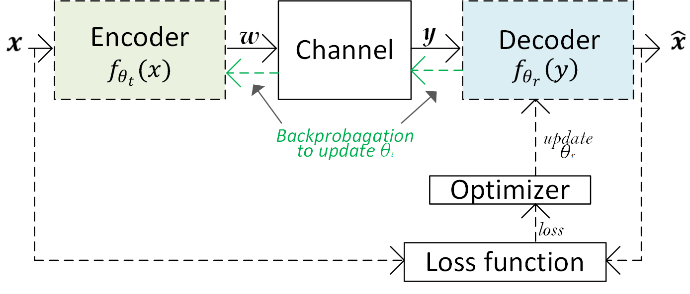
Figure 6: Backpropagating gradients for training the encoder to achieve AE end-to-end training

VIII-A Determining Differentiability

To determining whether a channel is differentiable depends on the specific characteristics of the channel model. a differentiable function (channel) typically has a tangent line at every point along its graph. If the tangent exists, the function is continuous, and its derivative exists, making it differentiable [51]. Here are some considerations:

• Mathematical formulation: If the channel can be described by a mathematical function, such as linear channel, AWGN, or Rayleigh fading, it is likely to be differentiable. For example, the AWGN channel can be expressed as $y=x+n$, where $y$ is the received signal, $x$ is the transmitted signal, and $n$ is the noise. This channel is differentiable because its behaviour can be expressed as a continuous function.

• Discrete Effects: Non-differentiability often arises from discrete effects, such as quantisation and modulation. If the channel introduces discrete operations, such as a threshold, it may not be differentiable. In such cases, alternative training methods such as reinforcement learning are needed.

• Noise Models: Noise models matter. AWGN is differentiable due to its Gaussian noise, but other noise models, such as impulsive noise, may not be.

• Physical limitations: Real-world channels have physical constraints, such as power limits or bandwidth limits. These constraints affect differentiability. For instance, clipping can make a channel non-differentiable.

VIII-B Solution Approaches for Non-differentiable

A key challenge in end-to-end AE learning for communication systems is the need for a differentiable channel model to enable transmitter training through backpropagation [52]. End-to-end training becomes feasible by treating the channel as a differentiable component. However, accurate differentiable channel models are often unavailable in practical scenarios, leading to performance degradation when deployed. If the channel is non-differentiable, due to nonlinearities or discrete effect, alternative approaches are needed, such as:

• Alternating training algorithm: The idea behind this is to optimise the transmitter and receiver independently. The iterative optimisation process involves alternating between optimising the receiver with a fixed transmitter and subsequently optimising the transmitter with a fixed receiver. This approach aims to enhance the overall system performance through this iterative refinement. This can be achieved through an alternating optimisation approach, where the receiver is trained using supervised learning while the transmitter is optimised using reinforcement learning [53, 54].

• Differentiable DSP algorithms: An end-to-end differentiable AE channel require all components, including DSP algorithms, to be differentiable to enable gradient-based optimisation. Traditional DSP algorithms often incorporate non-differentiable operations, hindering their direct integration into the differentiable channel. Therefore the authors of [55] proposed to modify blind phase search (BPS) algorithm and make it differentiable to include it in the end-to-end constellation shaping.

• Learning stochastic channel model: This approach involves learning a surrogate channel model, either through supervised learning [56] or adversarial methods [57] The key idea is to learn a differentiable generative model of the channel in the form of a GAN, which can then be used to train the AE, and to approximate end-to-end channel responses. The learned model is subsequently employed to train the transceiver. This enables direct optimisation of the modulation and encoding components within an end-to-end AE model. The accuracy of this learned model is crucial for the overall system performance. In [58], a channel-sensitive AE (CSAE) incorporates a pre-trained conditional GAN (CGAN) to model optical fibre communication systems with varying impairments.

• Two-phase training strategy [52]: With this approach, first train the AE using a channel model designed closely to the real channel such as a stochastic channel model. Upon deploying the trained model for real-wold transmission, performance is contingent on the model’s accuracy. To mitigate this, based on measurement data a find-tuning phase focusing exclusively on the receiver part of the AE, which lead to a sub-optimal training.

• Reinforcement learning-based approaches: the idea is to train an neural network (NN)-based transmitter using policy gradients while employing a non-differentiable receiver that treats detection as a clustering problem [59].

• Stochastic perturbation techniques: A gradient free optimisation techniques called Simultaneous perturbation stochastic optimisation has been proposed in [60]. it is a novel, single-stage approach to train deep learning-based communication systems directly in real-world channel environments. By circumventing the need for explicit channel modelling, this way leverages stochastic approximation to estimate gradients, enabling end-to-end optimisation.

• Gradient-free training method: It is a derivative-free optimisation method to eliminate the need for a differentiable channel model in AE training. This enables simultaneous optimisation of the encoder and decoder for arbitrary, even non-numerical, channel environments. The authors of [61] proposed the use of the cubature kalman filter (CKF) which offers gradient-free training while maintaining accuracy, thereby facilitating online adaptation.

  Figure 7: Solutions for Non-differentiable Channel

• Diffusion models: The idea is to the use of diffusion models (DMs) to accurately learn channel distributions. The work in [62] focusses on generative models and proposes an efficient training algorithm for end-to-end coded-modulation systems. DMs have demonstrated high sample quality and mode coverage in image generation, where the resulting differentiable channel model supports training neural encoders by enabling gradient-based optimisation.

• Genetic algorithms (GAs): While traditional end-to-end learning relies heavily on backpropagation, which requires the system to be differentiable, genetic algorithms offer an alternative optimisation method that does not rely on gradient information [63, 64, 65, 66].

  • optimisation without gradients: GAs optimise a population of solutions through evolutionary processes such as selection, crossover, and mutation. This optimisation process does not require the computation of gradients and can be applied to non-differentiable functions.

  • Fitness evaluation: In the context of an AE, the GAs can evaluate the fitness of each individual in the population based on how well the AE reconstructs the input data after it has passed through the channel. The fitness function can be designed to measure the reconstruction error or any other relevant performance metric.

  • Non-differentiable channels: If the channel in the communication system is non-differentiable, due to involving quantisation, discrete noise, or other non-continuous processes, traditional gradient-based methods fail to optimise the AE effectively. GAs, on the other hand, can still optimise the system by treating it as a black-box and relying on fitness evaluations rather than gradient information.

  • Population diversity: GAs maintain a population of potential solutions, which can help explore the solution space more thoroughly compared to gradient descent methods that might get stuck in local minima. This can be particularly beneficial in complex, non-differentiable landscapes.

IX AE Complexity

Computational complexity is essential for both the encoder and decoder components of AE-based systems. A practical approach involves counting floating-point operations (FLOPs) [67], which is commonly used to assess the computational performance of algorithms and hardware in machine learning. It measures the computational performance of algorithms and hardware, which is more practical for machine learning algorithms. Additionally, counting FLOPs for algorithm complexity has different advantages such as efficiency analysis of the algorithm, hardware benchmarking, and optimising the algorithm. In the context of AEs, FLOPs must be calculated for both the encoder and the decoder. For each layer, the number of FLOPs for matrix multiplication, bias addition and nonlinear activation functions should be considered as follows:

IX-A Matrix Multiplication

The AE encoder receives a one-hot vector $1_{l}\in\{0,1\}^{L}$ of length $L$. This input is then multiplied by a weight matrix $W\in R^{N\times L}$, where $N$ is the number of neurones in the layer. Following [67], the computational complexity of matrix multiplication between matrices $X$ and $Y$ with sizes ($a\times b$) and ($b\times c$) respectively, is given by ($2abc-ac$). Therefore, in the context of an AE layer with $N$ neurones, the number of FLOPs required is $N(2L-1)$.

IX-B Bias Addition

Each neurone is associated with bias addition represented by a vector $B\in R^{L}$, where $L$ is the number of neurones in a layer. Adding the bias term requires one FLOP per neurone. Therefore, the total number of FLOPs for both matrix multiplication and bias addition can be calculated as $N(2L-1)+L$.

IX-C Nonlinear Activation Function

Table  V provides a breakdown of the FLOPs counted for various activation functions in a layer with $N$ neurones. Appendix  A details the specific calculations for each activation function.

In summary, formula $N(2L-1)+L+F_{act}$ can be used to calculate the total number of FLOPs, where $F_{act}$ the FLOPs associated with the chosen activation function based on Table  V.

TABLE V: Number of FLOPs of Activation Functions

Activation Functions	FLOPs
ReLU	$N$
ELU	$8N$
Leak ReLU	$2N$
Tanh	$13N$
SELU	$9N$
Swish	$8N$
Softmax	$7N-1$
Sigmoid	$7N$

X Literature Review of leveraging AE in Communication systems

Recent research on AE applications in communication systems focusses mainly on the following key research directions.

• System-Level Design: focus on optimising communication systems holistically. Efforts in transceiver design aim to develop advanced architectures for efficient multiuser and varying channel scenarios. Complementing this is the push for end-to-end learning frameworks for complex scenarios, which unify traditionally separate processes such as channel coding, modulation, and equalisation. Research into high-performance code design explores capacity-approaching codes and innovative loss functions to improve power efficiency and communication reliability. Meanwhile, waveform optimisation leverages AEs to generate waveforms that meet constraints, ensuring high spectral efficiency and robust performance.

• Channel and Signal Processing: Efforts address specific channel impairments and improve signal processing. Channel modelling mitigates issues such as fading and phase noise. DSP techniques improve equalisation and noise mitigation. Non-differentiable channels are tackled with GANs, reinforcement learning, and Kalman filters. Robust transmission ensures reliable performance in noisy and interference-prone environments.

• Technology-Specific Applications: AEs are adapted for various communication technologies. MIMO systems use AEs for beamforming, CSI feedback, and interference management. OFDM systems address synchronisation, PAPR, and waveform optimisation. CRNs benefit from improved spectrum sensing and interference mitigation. Optical systems are used to deal with turbulence and absorption, while quantum communication employs hybrid AEs to handle noise and improve performance.

• Functional Improvements: It focusses on redefining core communication tasks. Channel coding enhances reliability in complex scenarios. Modulation and demodulation adapt jointly to impairments. Semantic communication prioritises meaning over raw data, improving efficiency and handling semantic noise.

• Computational and Practical Constraints: It focusses on resource efficiency and real-world applications. Resource-constrained systems optimise AE performance for hardware such as FPGAs. Hybrid learning strategies combine traditional methods with deep learning. AE interpretability improves transparency and scalability under varying conditions.

• Emerging Applications and Novel Methods: AEs are applied to novel domains. Specialized applications include radar systems, underwater communication, and RIS networks, focussing on beamforming and signal reconstruction. New methods improve BER, spectral efficiency, and resilience in challenging environments.

Figure 8: Thematic Taxonomy of AE-based Communication Systems

Fig. 8 shows a thematic taxonomy for research related to AE in communication systems. It presents a hierarchical structure, starting from categorising various research issues, channel type modelled, AE architecture used in the current literature, including type of layers, loss functions, and application areas where the model has been applied, like Wireless Communication (WC), Optical Communication (OC) including Visible Light Communication (VLC), Optical Wireless Communication (OWC), and Underwater Optical Communication (UOC).

X-A Wireless Communication

X-A1 Transceiver Design

This section explores various aspects of AE technologies-enhanced transceiver design systems. Notable studies focus on handling channel variations, optimising constellations under specific channel models, and improving performance in complex environments such as Rician flat-fading channels, nonlinearities, multipath fading, and MIMO broadcast interference channels. Key studies highlight approaches for waveform optimisation under constraints and the use of advanced neural network designs, such as ResNet blocks, to enhance system performance under varied channel conditions.

MIMO Systems

Numerous scholarly articles have examined the application of an AE-based MIMO communication system for transceiver design. A system designed to handle random variations in the channel, particularly focussing on MIMO systems, multi-dimensional constellations (MDC), and Rician flat fading channels, is proposed in [68]. Dorner et al. [69] introduced a bit-wise AE that can achieve shaping gains in MIMO systems by considering the Gaussian channel model with ergodic Rayleigh channel matrices. It deals with the curse of dimensionality when scaling the architecture for larger bit configurations (beyond 8 bits) and the need for constellation optimisation tailored to specific receiver algorithms to enhance performance. Optimisation of communication reliability in reconfigurable intelligent surface (RIS)-assisted MIMO systems is explored in [70]. It replaced the transceiver and the RIS model with three fully-connected neural network (FCNN) models and jointly trained the proposed system to minimise BER. Furthermore, Song et al. [71] analysed how AE for interference channels learns to avoid interference in a rotated reference frame, with AWGN, open-loop MIMO, closed-loop MIMO, and MIMO broadcast interference channels.

OFDM Systems

An AE-based approach to optimise OFDM systems for transceiver design. Felix et al. [72] examined the ability of the AE-based OFDM system to handle nonlinearities and synchronisation issues without explicit compensation algorithms. It used a WiFi-inspired stochastic channel model derived from a Proakis type C tap-delay-line model, with AWGN and multipath fading. Aoudia et al. [73] advanced the joint design of transmit and receive, with constellation geometry and bit labelling to eliminate orthogonal pilots in scenarios with frequency and time-selective fading channels. The proposed AE used ResNet blocks with separable convolutional layers and the ReLU activation function, along with a separable two-dimensional (2D) convolution output layer. The design of OFDM waveforms that meet specific constraints on PAPR and ACLR has been addressed in [24, 41, 25]. The proposed AE model used ResNet blocks, which in turn used separable convolutional layers and a convolutional output layer. The BCE loss function designed to maximise achievable information rates while satisfying PAPR and ACLR constraints is suggested for designing OFDM waveforms. The first two papers [24, 41] employed ResNet blocks with ReLU activation, while the third paper [25] substituted ReLU with ELU to address the problem of vanishing gradients. In the same direction, Marasinghe et al. [74] addressed the key issue of Constellation Shaping under phase noise (PN) impairment for Sub-THz Communications. The study used the AWGN channel model, which simplifies the analysis by assuming perfect channel equalisation while focussing on PN impairment. The loss function is formulated in an augmented Lagrangian form, which is used to optimise the constellation design robust to PN while maintaining low PAPR.

TABLE VI: Comparison of AE-based models for Transceiver Design

Ref.	Main Contribution	Model(s) Used	Dataset/Data type/Channel model	Best performance value	Limitation
[24]	PAPR reduction	ResNet blocks (sep. conv, ReLU)	Simulated, AWGN	1.4 dB difference at CCDF $10^{-3}$	BCE computation complexity
[25]	PAPR, ACLR reduction	ResNet blocks (sep. conv, ELU)	Synthetic, AWGN	8.5 dB PAPR reduction	Constraint evaluation complexity
[27]	Non-differentiable channel	Tx: Dense (ELU), Rx: Dense (ReLU), RBF	Synthetic, AWGN, RBF	Comparable to supervised	Slower convergence on AWGN
[41]	Joint Tx/Rx, constellation, labelling	ResNet blocks (sep. conv, ReLU)	Simulated, AWGN, multipath	ACLR $-$29.95 dB, PAPR 5.60 dB	NN architecture complexity
[68]	Adapt to random fading	Symbol differentiation, dense	Rician fading, AWGN	Superior SER in high SNR	Optimised for specific channel
[69]	Curse of dimensionality	Bit-wise AE, dense (ReLU)	Complex Gaussian	APP receiver for k=8	Scalability limitations for k¿8
[70]	RIS-assisted MIMO reliability	Fully connected (ReLU)	200k symbols, AWGN	Lowest BER across SNR	Single deterministic channel realisation
[71]	Avoid interference	Dense Layer, geometric shaping	Rayleigh fading, AWGN	Outperforms Alamouti	Error floor at high SNR
[72]	Joint Tx/Rx optimisation	Dense (nonlinear), seq. detector	Complex-valued, WiFi-inspired	Improved block error rate (BLER)	Complexity of analysing AE-based system
[73]	Pilot signal reduction	ResNet blocks (sep. conv, ReLU)	Realistic wireless, time/freq-selective	BER close to perfect knowledge	Practical implementation challenges
[74]	Mitigate hardware impairments	SC-FDE BMD	AWGN, Wiener phase noise	0.3 dB BLER improvement	Limited to SC-FDE, AWGN channel

X-A2 Channel Coding and Decoding

The importance of AEs for channel coding and decoding stems from their potential to redefine communication system design through end-to-end optimisation. Traditional coding approaches often rely on separate stages for modulation and channel coding, optimised under conventional assumptions. However, such designs struggle to adapt to complex or non-conventional channel conditions, leading to suboptimal performance. AEs, using deep learning, integrate channel coding and decoding within a unified framework. By learning directly from data, they overcome limitations of traditional methods, achieving near-optimal performance in challenging environments like non-AWGN channels, mismatched conditions, or inter-symbol interference. Studies such as [75] and [76] demonstrate how AEs improve robustness, reliability, and efficiency, paving the way for advanced adaptive communication systems.

Turbo AEs and Hybrid Designs

Jiang et al. [75] proposed the Turbo AE (TurboAE), which attained state-of-the-art performance in conventional AWGN channels for moderate block lengths and surpassed traditional codes such as LDPC and Turbo codes in non-standard settings like additive T-distribution noise, thereby demonstrating the potential of deep learning techniques to automate the design of channel coding design. Based on this, Jiang et al. [77] introduced TurboAE-MOD, which combines channel coding and modulation within an end-to-end framework. This approach exhibited enhanced reliability and robustness, especially under non-Gaussian channel conditions, when compared with conventional modulation techniques.

Channel AEs and Model-Free Approaches

Zou et al. [76] provided a detailed overview of channel AEs, highlighting the distinctions between model-free approaches (e.g., GAN-CAE) and model-assumed methods (e.g., AWGN-CAE), both of which demonstrated competitive BLER performance, although model-free methods required extended training due to their reliance on surrogate models. Complementing this, Xu et al. [78] evaluated end-to-end AEs in the AWGN and Rayleigh channels, achieving performance comparable to Hamming codes, while exhibiting improved robustness in practical scenarios characterised by channel mismatches, notably within urban and suburban environments.

AEs for ISI Channels and Blind Equalisation

Zhang et al. [79] introduced a Bi-GRU-based AE tailored for ISI channels, offering flexible coding rates and outperforming convolutional and LDPC codes in low SNR regimes. Nevertheless it requires further enhancements at high SNR. Similarly, Caciularu et al. [80] introduced VAE Equalisers specifically for the purpose of blind equalisation, which resulted in considerable enhancements in SER and exhibited strong performance in nonlinear ISI channels, thus outperforming established methodologies such as Turbo EM.

Innovations in Joint Source-Channel Coding (JSCC)

Saidutta et al. [81] developed a VAE-based JSCC scheme, which achieved near-optimal SDR for Gaussian sources while maintaining robustness across different channel conditions. The approach also demonstrated superior performance on image datasets compared to traditional methods.

Specialized AE Implementations

Xu et al. [82] introduced a multi-carrier turbo-style AE for OFDM systems, which delivered significant performance improvements over conventional OFDM and OFDM-IM while allowing seamless integration with existing systems. Rajapaksha et al. [83] developed a low-complexity AE that outperformed convolutional coding in the low to moderate SNR ranges, which achieved notable parameter reduction. Furthermore, Balevi et al. [84] proposed a system combining turbo codes with AE for one-bit quantised receivers, which achieved superior BER and enhanced computational efficiency compared to traditional coding methods.

Advancements in Capacity-Approaching Codes

Letizia et al. [85] proposed an AE loss function that incorporates mutual information to design capacity-approaching codes. The study highlighted advances in BLER and mutual information optimisation, although specific performance values depend on channel setup.

Robust Transmission of Latent Representations

Khan et al. [86] combined basic and denoising AE to enhance robustness in transmitting latent image representations under noise and quantisation. This approach improved classification accuracy and reconstruction quality under challenging conditions.

TABLE VII: Comparison of AE-Based Models in Channel Coding and Decoding

Ref.	Main Contribution	Model(s) Used	Dataset/Data Type	Best Performance Achieved	Limitation
[75]	Proposes Turbo AE with state-of-the-art performance for conventional and non-conventional settings	TurboAE	conventional and Non-AWGN Channels	BER $<10^{-5}$ at high SNR; Outperforms benchmarks in reliability for non-conventional channels	Slightly worse performance than LDPC and Polar codes at high SNR
[76]	Discusses model-free and model-assumed channel AEs, with extensive performance comparison	Channel AEs (GAN-CAE, RL-CAE)	AWGN, Rayleigh Channels	Comparable BLER under AWGN and Rayleigh channels; Model-free methods robust to complex channels	Model-free methods require more training epochs
[79]	Proposes a flexible AE for coding with arbitrary rates	Bi-GRU-based AE	ISI Channels, AWGN	Outperforms convolutional and LDPC codes in low SNR	Performance degrades in high SNR
[80]	Introduces a VAE-based approach for blind equalisation and decoding	VAE	Linear/Nonlinear ISI Channels	BER $10^{-3}$ at SNR 6 dB; Robust against nonlinear channels	Computational complexity increases with channel impulse length
[82]	Introduces a flexible MC-AE for integration with any channel coding	Turbo-style Multi-Carrier AE	OFDM Systems	Achieves frequency diversity gain and surpasses OFDM-IM performance	High computational cost due to multi-stage learning
[81]	Proposes a JSCC approach using VAE for various source distributions	VAE with Mixture-of-Experts	Gaussian and Laplace Sources; AWGN Channels	SDR within 0.96 dB of Shannon limit for Gaussian sources	Performance varies with source-channel mismatch
[85]	Incorporates mutual information in loss for capacity-approaching codes	Capacity-Approaching AE	Unknown Channels	Significant advancements in BLER and mutual information	Results rely on channel assumptions
[83]	Proposes a low-complexity AE for coded systems	Low-Complexity AE	AWGN Channels	Better BER than 16-QAM in low SNR; MER $<10^{-4}$ at 10 dB	Performance lags in high SNR
[77]	Combines TurboAE and feed-forward NN for modulation coding	TurboAE-MOD	AWGN, Additive T-Distributed Noise	Comparable to Turbo codes at moderate block lengths; Superior in non-AWGN channels	Degrades in high SNR
[86]	Improves robustness against noise and quantisation for image transmission	Basic AE + Denoising AE	Latent Representations of Images	Maximum CA and minimum MSE with latent vector size 20, 4 bits	High sensitivity to quantisation
[84]	Combines Turbo code and AE for one-bit quantized receivers	ConvAE with Turbo Code	AWGN Channels	Lowest BER for 4-bit transmission; Processes batch in 12.2 µs	Training requires careful tuning
[78]	Evaluates AE performance across channel types	End-to-End AE	AWGN, Rayleigh, Urban/Suburban Channels	Comparable BLER to Hamming codes; Robust under channel mismatch	Slightly worse in high-speed channels

X-A3 Modulation and Demodulation

AEs have emerged as transformative tools in wireless communication, particularly for tasks such as modulation and demodulation. These deep learning models replace traditional transmitter and receiver modules with an encoder-decoder architecture, enabling end-to-end optimisation of communication systems. Unlike conventional methods that optimise modulation and coding separately, AEs jointly learn these processes, allowing them to dynamically adapt to channel impairments and environmental variations. This holistic approach not only improves the efficiency and resilience of the system, but also lays the foundation for robust communication systems capable of addressing the complexities of modern wireless networks.

Signal Transmission and Encoding

Building on this foundational concept, Park et al. [87] demonstrated the potential of AEs for signal transmission in sonobuoy systems. Their approach encoded signals into low-dimensional latent vectors, which reduced data volume by 100 times while enhancing security. Reconstruction errors were kept below 4%, with effective noise reduction achieved using a denoising AE, resulting in a MSE of 0.000238 with the AE model.

Spatial Modulation (SM)

Shrestha et al. [88] tackled challenges in SM by embedding antenna index signatures within AE frameworks, which significantly improved signal robustness under high antenna correlation and achieved BLER and power efficiency gains of 18$-$24 dB in Rician channel setups.

SNR Improvement

Further advancing the field, Duan et al. [89] developed a dual-residual denoising AE with channel attention (DRdA-CA), which achieved substantial improvements in SNR, such as a gain of 8.38 dB for 16-QAM, and reduced BER by up to 63.5% . Zhu et al. [90] complemented this by presenting a stacked denoising AE for rapid and accurate modulation classification, outperforming traditional methods, especially in noisy environments. Expanding on SDAE applications, Bogale et al. [91] applied this technique to FSO communications for signal denoising and used a deep belief network (DBN) for wavelength demodulation, which achieved notable SNR improvements of +22 dB and high wavelength demodulation accuracy of 0.06 nm.

Modulation Classification

In terms of modulation classification, Ali et al. [92] introduced an AE with non negativity constraints, which achieved 100% classification accuracy at high SNR (10$-$15 dB) and demonstrated robustness under fading conditions. This approach outperformed traditional sparse AEs in both reconstruction error and classification accuracy. Based on this, Ke et al. [93] designed a LSTM-based denoising AE for radio technology and modulation classification, achieving a high accuracy of 96.56% at high SNR in the RadioML2018.01A dataset. Their model also demonstrated computational efficiency, operating effectively on low-cost platforms such as the Raspberry Pi 4.

Demodulation and Signal Reconstruction

Finally, Zhang et al. [94] introduced hybrid feature-modulated AEs to improve the demodulation of high-frequency information in channel-modulated polarisation imaging. Their method achieved notable improvements in metrics such as PSNR (e.g. $+$ 180% for S3) and SSIM scores, which proved to be effective for simulated and real-world images. Morocho et al. [39] further showcased the versatility of AEs by developing an end-to-end communication system that replaced traditional transmitter and receiver tasks. Their approach optimised system operations and was effectively adapted to channel impairments, highlighting the broad applicability of AE frameworks in communication systems.

TABLE VIII: Comparison of AE-Based Studies for Modulation and Demodulation

Ref.	Main Contribution	Model(s) Used	Dataset/Data Type	Best Performance Value	Limitation
[39]	Joint optimisation of transmitter and receiver tasks for adaptable communication systems.	End-to-End AE	Single-antenna systems with channel impairments	Demonstrated flexibility in handling channel impairments.	Lack of quantitative performance metrics for comparison with conventional systems.
[87]	Signal transmission with reduced data volume (100x reduction) and enhanced security using low-dimensional latent vectors.	AE, Denoising AE	Sonobuoy signal data (simulated)	MSE: 0.000238, 100x data reduction with ~4% reconstruction error.	focussed on specific sonobuoy environments, limiting generalizability to other systems.
[88]	Improved signal robustness under high antenna correlation with phase-shift keying and antenna index embedding.	AE Frameworks with Antenna Index Embedding	MIMO spatial modulation scenarios	18$-$24 dB gain in BLER and power efficiency (Rician factor of 20 dB).	Limited testing under other channel conditions or configurations.
[90]	Automated modulation feature extraction for rapid and high-accuracy classification.	Stacked Denoising AE	Synthetic modulation signals	Superior accuracy and speed compared to conventional methods in noisy conditions.	Lack of real-world signal testing and reliance on synthetic data.
[89]	Enhanced SNR and reduced BER with improved feature extraction and reconstruction quality.	DRdA-CA	Eight modulation types (e.g., 16QAM, 64QAM)	SNR improvement: 8.38 dB for 16QAM, BER reduction up to 63.5%.	High computational complexity may limit real-time deployment.
[92]	High classification accuracy under fading and noisy conditions with reduced reconstruction error.	AE with non negativity Constraint	Fourth-order cumulants of modulated signals	100% accuracy at 10-15 dB SNR, 86% at 0 dB SNR.	Limited scalability to higher-dimensional or diverse datasets.
[94]	Effective demodulation of high-frequency information with improved image quality.	Hybrid Feature Modulated AE	Channel modulated polarisation imaging data	PSNR improvement: +180% (S3), SSIM: 0.9665.	Limited exploration of diverse imaging scenarios beyond polarisation imaging.
[91]	Enhanced denoising and wavelength demodulation for FSO links under turbulence.	SDAE, DBN	FSO communication signals with real noise	SNR improvement: +22 dB, Wavelength accuracy: 0.06 nm.	Dependency on specific FSO setups; generalisation to other noise types unverified.
[93]	Efficient radio technology and modulation classification on low-cost platforms.	LSTM Denoising AE	RadioML2018.01A, Real-time PSD data	96.56% classification accuracy at high SNR, 4.3x faster classification speed on Raspberry Pi 4.	Limited evaluation for advanced modulation schemes or other radio datasets.

X-A4 Cognitive Radio Networks (CRNs)

Deep AEs improve CRN by improving spectrum sensing and interference mitigation, allowing efficient and adaptive communication in dynamic environments. For spectrum sensing, AEs extract essential features from signals, detect anomalies, and identify underused spectrum bands, with Denoising AEs proving effective in reconstructing clean signals under noisy conditions. In interference mitigation, AEs learn to suppress interference, adapt modulation schemes, and reconstruct signals in multi-user scenarios, which showed their ability to predict interference levels and dynamically adjust communication parameters. By automating feature extraction, providing real-time adaptability, and handling complex multidimensional data, AEs optimise spectrum use and ensure reliable, interference-aware communication in CRNs.

Spectrum Sensing and Anomaly Detection

Abdalzaher et al. [95] proposed a deep AE-based framework called (DAE-TRUST), to detect malicious nodes in cognitive radio (CR)-enabled IoT networks. By improving cooperative spectrum detection, the system achieved 100% accuracy in detecting malicious secondary users under specific conditions, with slight reductions in challenging environments. Subekti et al. [96] presented a spectrum sensing method that combines a deep AE for feature learning and an SVM for classification. This approach achieved up to 95% sensing accuracy in distinguishing primary and secondary users. Similarly, Nallarasan et al. [97] used AEs to detect random jamming attacks in cognitive radio IoT (CRIoT) networks, which achieved 89% detection precision by modelling jamming as an anomaly detection problem.

Signal Classification and Modulation Recognition

Liu et al. [98] introduced a stack hybrid AE framework for industrial CRNs, which achieved 97.75% classification accuracy in high SNR environments and thus outperformed other methods such as Capsule Networks. Zhu et al. [99] proposed using stacked denoising AEs for modulation classification, which achieved 97% accuracy at 5 dB SNR and surpassed traditional maximum likelihood methods in both classification accuracy and execution time efficiency.

Radio Map Estimation and Denoising

Teganya et al. [100] developed a deep-completion AE for estimating radio occupancy maps, which learnt spatial propagation patterns with fewer measurements compared to traditional methods. Almazrouei et al. [101] demonstrated the efficacy of convolutional denoising AEs in denoising radio signals, which achieved 96% accuracy at SNR = 0 dB and with robust performance under varying channel conditions.

Dynamic Interference Management and Beyond-5G

Wu et al. [102] proposed an AE based on adaptive deep learning (ADL) to manage dynamic interference in multi-user Gaussian channels, which significantly reduced BER and SER in strong interference scenarios. This approach enables adaptable constellations for 5G and beyond communication systems and demonstrated robustness in extreme interference conditions.

TABLE IX: Comparison of Studies on CRNs Using Deep AEs

Ref.	Main Contribution	Model(s) Used	Dataset/Data Type	Best Performance	Limitation
[95]	Malicious node detection in CR-assisted IoT	DAE-TRUST	IoT network data	100% accuracy in line-of-sight scenarios	Reduced accuracy in challenging environments
[96]	Spectrum sensing for CR systems	Deep AE + SVM	Spectrum sensing data	95% sensing accuracy	Limited to multi-radio environments
[97]	Jamming attack detection	AE	CRIoT network data	89% detection accuracy	Less effective for continuous jamming
[98]	Signal classification in ICRNs	Stack Hybrid AE	Industrial wireless signals	97.75% accuracy in high SNR	Lower performance in highly uncertain conditions
[99]	Modulation classification	Stacked Denoising AE	Modulation data	97% accuracy at 5 dB SNR	Higher complexity in dense symbol sets
[100]	Efficient radio occupancy map estimation	Deep Completion AE	Radio map data	High accuracy with minimal data	Generalization to unseen environments
[101]	Radio signal denoising	Convolutional Denoising AE	IEEE 802.11 signal data	96% accuracy at 0 dB SNR	Performance drops at very low SNR
[102]	Interference mitigation for beyond-5G systems	Adaptive DL-based AE	Multi-user Gaussian channel data	Significant BER/SER improvement	Higher complexity in real-time adaptation

TABLE X: Comparison of studies on deep AE-based methods for MIMO systems

Ref.	Main Contribution	Model(s) Used	Dataset/Data Type	Best Performance	Limitation
[82]	Flexible integration of DNN with channel coding for iteration gain	Turbo-style Multi-Carrier AE	OFDM systems	Substantial performance gain over conventional OFDM	Complexity in soft-decision integration with channel decoding
[103]	Introduced AE-based MIMO systems with improved BER	BWAE-MIMO, SWAE-MIMO	Simulated MIMO systems	Achieved BER comparable to MIMO-ML with RTN detector	Limited evaluation on specific antenna configurations
[104]	Variational AE-enhanced DNN for MIMO signal detection	VAE-DNN-Det	Simulated wireless networks	1 dB SNR gain over traditional methods	Performance depends on channel condition spectrum
[105]	Addressed feedback delay and errors in CSI feedback	Deep AE	Frequency division duplex (FDD) MIMO systems	Improved normalized MSE and robustness to feedback errors	Focused on specific feedback errors and delay cases
[106]	Joint channel estimation, feature extraction, and symbol detection with AEs	AE-based DNN	Simulated MIMO channels	Significant BER gains in high channel correlation scenarios	Complexity of training deep networks for MIMO systems
[107]	VAE-based deep learning for signal detection with reduced runtime	VAE	MIMO-OFDM-IM systems	BER performance comparable to traditional detectors with lower runtime	Requires offline training with simulated datasets
[108]	Embedded singular vectors in DAE for enhanced BER	SVD-embedded DAE	Simulated MIMO systems	BER improvement by 10-18x over linear precoding at SNR of 10dB	Limited to linear precoding scenarios
[102]	Adaptive AE for dynamic interference management in beyond-5G systems	ADL AE	Multi-user Gaussian interference channels	2 dB improvement in BER over conventional schemes	Performance highly dependent on interference estimation
[109]	AE-based intelligent hybrid beamforming for mmWave systems	AE-HB	mmWave MIMO systems	Over 3 dB BER improvement over linear beamforming	Limited evaluation on specific mmWave configurations
[110]	end-to-end learning approach for uplink distortion compensation	end-to-end AE	Multi-user MIMO uplink channels	Near-linear SER performance under Rayleigh fading channels	Focused on high-power amplifier distortions
[111]	Efficient CSI feedback with robustness to noise	PRVNet (VAE-based)	Indoor and outdoor FDD-MIMO scenarios	NMSE: $-27.7$ dB (indoor), $-13.9$ dB (outdoor) at CR=1/4	Limited to feedback channels with specific compression ratios
[112]	Improved relay quantization algorithms with BER enhancements	APQNN	Simulated relay systems with multiple antennas	BER $\approx 10^{-3}$ at SNR=12 dB with $q=8$ bits	Increased computational complexity due to neural network-based relay
[113]	Joint quantization and compression for CSI feedback	AE with entropy bottleneck layer	Indoor (5.3 GHz) and outdoor (300 MHz) CSI feedback	NMSE: $-24$ dB (indoor), $-13$ dB (outdoor) at BPP=3.0	Requires specific tuning for optimal entropy bottleneck performance
[114]	Mitigation of adversarial attacks on power allocation models	Denoising AE	Adversarial attack simulations for massive MIMO	Retained accurate performance across threat models	Limited application outside adversarial contexts
[115]	Joint optimisation of RIS and transmitter-receiver pairs	RIS-aided AE (Encoder-Decoder with RIS)	Simulated scenarios with obstruction losses	SER: 18 dB gain at $l_{o}=10$ dB, SER=$10^{-5}$	Limited evaluation in scenarios with dynamic environmental changes
[116]	Joint transceiver and ADC design optimization	AE with optimized ADCs	MIMO Rayleigh fading channels	12 dB gain at BLER=$10^{-2}$, 1 dB loss at BLER $\leq 10^{-3}$	Requires accurate ADC modeling for optimal results
[117]	Multi-objective optimization for PAPR, BER, and spectral performance	Convolutional AE	Simulated 16-QAM, 4×4 MIMO configurations	PAPR reduction: 4 dB at CCDF=$10^{-3}$	Computational overhead for multi-objective optimization
[118]	Energy-based AE for multiuser noncoherent systems	NC-EA	Multicarrier SIMO fading channels	BLER=$10^{-3}$ with 8 dB gain (single-user), 6.5 dB (multi-user)	Performance depends on accurate sub-carrier power allocation
[119]	Improved target detection accuracy over conventional CFAR	AE replacing CFAR	FMCW radar system simulations	Correlation coefficient $\geq 0.73$ with actual target data	Limited to automotive radar systems
[120]	Interference-aware constellations with adaptive shaping	DAE for Z-interference channels	Simulated ZIC scenarios	BER reduction: up to 2 orders of magnitude under imperfect CSI	High complexity for dynamic interference adaptation
[121]	Improved BER and SNR performance for MIMO detection	DNN-Det-VAE	MIMO setups (64-QAM, 256-QAM)	SNR gain: 1 dB at BER=$10^{-5}$ (4×4 MIMO, 64-QAM)	Limited gains in high SNR conditions compared to advanced methods

X-A5 MIMO

In the realm of modern wireless communication, MIMO technology has emerged as the cornerstone for achieving higher data rates, improved spectral efficiency and reliability. As demand for high-performance systems grows with the advent of 5G and beyond, traditional signal processing techniques often fail to address the complexity and dynamic nature of MIMO systems. This has paved the way for the integration of advanced deep learning methodologies, particularly deep AEs. Deep AEs, known for their ability to extract meaningful representations and compress high-dimensional data, offer a promising solution to tackle various challenges in MIMO systems. By treating the communication process as an end-to-end optimisation task, AEs can jointly optimise transceiver design, CSI feedback, and interference mitigation. This approach not only simplifies system architectures but also significantly enhances key performance metrics such as BER, spectral efficiency, and energy consumption. The application of deep AEs spans a wide range of MIMO functionalities, including hybrid beamforming, reduction of PAPR, and robust detection under adverse channel conditions.

Signal Detection and Processing

Several recent studies have explored the use of AE-based frameworks and deep learning techniques to improve signal detection and processing in MIMO systems. Bui et al. [103] introduced two innovative systems, BWAE-MIMO and SWAE-MIMO, which use AE to improve signal detection performance. Among these, the BWAE-MIMO system, equipped with the radio transformation network (RTN) detector, achieved BER performance comparable to the maximum likelihood detection (MLD) approach in 2×2 MIMO configurations. This highlights the potential of AEs to compete with traditional methods while leveraging the advantages of deep learning. Building on this concept, Omondi and Olwal [121] proposed the DNN-Det-VAE architecture, which incorporated VAEs into a deep learning framework for MIMO detection. Their method demonstrated a SNR gain of 1 dB in 4×4 MIMO setups with 64-QAM and 256-QAM constellation formates. The approach exhibited superior BER performance compared to traditional methods such as zero force (ZF) and minimum MSE, which demonstrated its effectiveness under challenging channel conditions. In a similar vein, Zhao et al. [107] developed a VAE-based signal detection method adapted to MIMO-OFDM-IM systems. Their approach achieved BER performance that was not only close to existing hand-crafted detection algorithms but also featured reduced runtime, thus underscored the efficiency of deep learning-driven solutions. Kavitha et al. [106] explored the application of AE-based DNN for MIMO signal processing. Using the dimensionality reduction capabilities of AEs, their framework demonstrated robustness to channel impairments and delivered significant performance improvements in BER and spectral efficiency compared to conventional MIMO detection techniques. This study also highlighted the scalability and flexibility of deep learning approaches to address complex MIMO communication challenges.

Hybrid Beamforming and Advanced Architectures

Tao et al. [109] introduced an innovative AE-based hybrid beamforming method (AE-HB) for mmWave. By mapping the hybrid beamforming problem to an AE neural network, their approach transformed the traditionally non-convex optimisation problem into a neural network training process. This method demonstrated a significant 3 dB improvement in BER compared to conventional linear beamforming systems, thus showcased the potential of using neural networks to optimise hybrid beamforming in next-generation communication systems. Building on the integration of deep learning into MIMO systems, Cherif et al. [110] developed an end-to-end learning approach aimed at mitigating nonlinear distortions, such as those introduced by high-power amplifiers in massive MIMO systems. Their framework used deep neural networks and AEs to jointly optimise the transmitter and receiver under Rayleigh fading conditions. The proposed approach achieved near-linear SER performance at high SNRs with 16-QAM modulation, which significantly outperformed traditional distortion mitigation techniques. Together, these studies highlight the transformative potential of AE-based methods to address complex challenges in MIMO communication, including beamforming and nonlinearity compensation, while improving system reliability and efficiency.

Channel State Information (CSI) Feedback

Jang et al. [105], Hussien et al. [111], and Ravula et al. [113] each addressed the challenge of CSI-efficient feedback in MIMO systems through innovative deep learning approaches. The first proposed a deep AE-based method that significantly reduced normalised MSE and demonstrated robust performance under feedback errors and delays, which ensured reliable CSI reconstruction. Building on this, the later introduced PRVNet, a VAE-based model optimised for high compression scenarios. PRVNet achieved exceptional NMSE values of $-27.7$ dB in indoor environments and $-13.9$ dB in outdoor settings in a compression ratio of 1/4, which outperformed many existing methods. Similarly, the latter proposed an entropy bottleneck layer within an AE-based feedback framework, which enabled joint optimisation of bit rate and distortion. This approach achieved NMSE values of $-24$ dB for indoor channels and $-13$ dB for outdoor channels at specific bit-per-pixel (BPP) values, which demonstrated superior reconstruction quality over traditional methods. Collectively, these studies highlighted the potential of AE and VAE-based techniques to improve CSI feedback efficiency and accuracy in diverse wireless environments.

Interference Mitigation and Robustness

Wu et al. [102] and Sahay et al. [114] explored innovative deep learning approaches to enhance interference mitigation and system robustness in wireless communication. The first proposed an adaptive AE designed for 5G and beyond systems, which effectively addressed dynamic interference challenges. Their method demonstrated robust BER performance, particularly in strong and very strong interference scenarios, which demonstrated adaptability to varying network conditions. The second, on the other hand, introduced a denoising AE aimed at countering adversarial attacks in massive MIMO power allocation systems. This approach was shown to be effective in various attack models, ensuring resilience and maintaining system performance even under adversarial conditions. Together, these studies highlighted the critical role of AE-based techniques in mitigating interference and enhancing the robustness of next-generation wireless systems.

Performance Optimisation for End-to-End Communication

Zhang et al. [108] and Van et al. [118] focused on optimising end-to-end communication performance in wireless systems using advanced deep learning frameworks. Zhang et al. introduced a singular value decomposition (SVD)-embedded deep AE for MIMO systems, which demonstrated significant BER improvements. Their approach achieved up to an 18-fold reduction in BER compared to traditional precoding methods at an SNR of 10 dB, which highlighted the potential for embedding mathematical transformations within AE structures. Van et al. developed a noncoherent energy AE (NC-EA) system for single-input multiple-output (SIMO) setups, which addressed both single-user and multi-user scenarios. The proposed NC-EA system achieved substantial SNR gains, including 8 dB for single-user configurations and 6.5 dB for multiuser systems at a BLER of $10^{-3}$. These advancements underscore the effectiveness of integrating deep learning into end-to-end communication design to achieve superior reliability and efficiency.

Specialized Applications and Novel Methods

Shin et al. [112] introduced the amplitude phase quantisation with neural networks (APQNN) framework for relay systems, which achieved significant BER improvements. Their approach demonstrated performance close to $10^{-3}$ BER at high SNR levels, which emphasised its effectiveness in the optimisation of the relay system. Similarly, Erpek et al. [115] developed a RIS-aided AE system for joint transmitter-receiver optimisation. This method achieved substantial reductions in SER, with performance gains of up to 18 dB under high obstruction losses, which highlighted the potential of RIS in improving end-to-end communication efficiency. Ye et al. [116] proposed an AE-based MIMO communication framework that incorporates end-to-end optimised analogue-to-digital converters (ADC). This approach resulted in a gain of 12 dB at a BLER of $10^{-2}$, closely matching the unquantified lower bound baselines. In another innovative effort, Huleihel et al. (2024) [117] introduced a convolutional AE framework for PAPR reduction in MIMO-OFDM systems. Their method achieved a 4 dB reduction in a complementary cumulative distribution function (CCDF) of $10^{-3}$, demonstrating effectiveness in optimising spectral and detection performance simultaneously. Further extending the applications of AEs, Kang et al. [119] replaced traditional constant false alarm rate (CFAR) algorithms with an AE-based approach in frequency-modulated continuous wave (FMCW) radar systems. The proposed method achieved a correlation coefficient of 0.73 or higher in the target detection results, which highlighted its robustness in signal processing tasks. Furthermore, Zhang et al. [120] proposed a deep AE-based architecture for Z interference channels. This innovative system achieved up to two orders of magnitude reduction in BER, particularly under imperfect CSI conditions of the channel, which demonstrated its resilience to interference and CSI estimation errors.

TABLE XI: Comparison of AE-based models in Optical Communication

Ref.	Main Contribution	Model(s) Used	Dataset/Data Type	Best Performance	Limitation
[26]	PAPR reduction	LSTM-AE	VLC DCO-OFDM, AWGN	4.2 dB at CCDF $10^{-3}$	Limited PAPR improvement
[48]	Accurate gradient estimation	Sigmoid/Softmax	Constellation points, AWGN	Near-optimal MI/GMI	Complexity for complex channels, large constellations
[122]	Improved BER	Dense (ReLU)	Binary vectors, AWGN	Better than half-rate 16-QAM	Idealized communication assumptions
[123]	Efficient transceiver design	SR-AE, DNN	Poisson Channel	DNN outperforms existing designs	SR-AE performance loss in some scenarios
[124]	Train in real channels, power control	VAE, Feedforward	AWGN, AIL, AICN, RBF	Faster training, lower BLER	Challenges at high dimensions
[125]	Scalable transceiver	AEGNN	AWGN, Multicolor VLC	Comparable SER to traditional methods	Relies on channel model assumptions
[126]	Channel attenuation	Fully connected	Underwater optical, AWGN	Best 16QAM performance	Sensitivity to channel conditions
[127]	Atmospheric turbulence	Symbol differentiation	Random messages, Rytov variance	12 dB improvement over PPM	ML receiver performance worse than DNN
[128]	BER degradation in unknown CSI	1D Conv (ELU)	Random bits, Gamma-Gamma	BER $10^{-5}$ at SNR 20.5 dB	Degrades with increasing turbulence
[129]	Adaptation to nonlinear fibre links	Dense (ELU)	AWGN, CD, KNL	High spectral efficiency gain	Training complexity
[130]	Amplification noise vs. nonlinearity	Dense (ReLU)	Differentiable fibre channel	0.13 bit/4D improvement	Model discrepancy
[131]	Dispersion-induced interference	FFNN, BRNN	Random messages, CD	Operation beyond 70 km	FFNN limitations
[132]	Dispersion-induced interference	SBRNN, FFNN	CD, memory effects	Transmission below 6.7% HD-FEC	Trained on specific channel models
[133]	Carrier recovery, channel estimation	VAE, 1D Conv (ELU)	Dual-polarisation, AWGN, ISI	VAE-based outperform CMA	Convergence issues at high symbol rates
[134]	Slow convergence of traditional methods	VQ-VAE	Unshaped 64-QAM, PDM	Frequency-domain VQ-VAE comparable to time-domain, outperforms CMA	ELBO computation challenges
[135]	Bootstrapping of blind equalizers	VAEflex	Linear frequency domain, AWGN, PMD	Highest BMI	Higher percentage of failed runs
[136]	Laser phase noise	Bit-wise (ReLU)	Simulated symbols, Wiener phase noise	0.1 bit/symbol gain	May not consistently outperform
[137]	Optimise constellation shaping	Bitwise	Synthetic datasets, Wiener phase noise	Improves 64-ary performance	Lack of detailed complexity analysis
[138]	Differentiable CPE	Fully-connected (ReLU)	Simulated signals, Wiener phase noise	µ = 4 provides best performance	Additional computational complexity
[139]	Differentiable channel model	Dense (ReLU)	AWGN, RBF, simplified fibre-optic	State-of-the-art hardware	Relies on accurate channel models
[140]	Design constellations for nonlinearities	Dense (SELU)	Nonlinear fibre channel, ASE noise	0.13 bit/4D gain	Model agnostic to embedded channel
[141]	Optimise transceiver chain	Fully-connected (ReLU)	Labelled input-output pairs	42 Gb/s at $<$ 6.7% HD-FEC	Sensitivity to distance variations
[142]	Optimise input probability distributions	Distance-agnostic AE	Experimental data, Generative model	Outperforms uniform distributions	Optimisation on specific model assumptions
[143]	Design techniques for optical channels	Dense (linear)	Simulated messages, AWGN	1 dB inferior to soft-decision decoder	Fails when both transmitters send same symbols
[144]	Long-distance atmospheric turbulence	Dense (ReLU)	AWGN, multipath fading	Outperforms conventional QAM	Suboptimal compared to global solution
[145]	Optimise geometric constellations	Dense (ReLU)	fibre channel with WDM	Up to 0.2 bits/symbol GMI gain	Implementation penalty

X-B Optical Communications

The existing research focussed on the application of deep learning techniques, particularly the use of AEs and VAEs in various optical communication systems, addressing unique challenges and proposing innovative solutions.

In the field of OWC, Si-Ma et al. [123] explored the use of AEs for the design of the SISO transceiver operating in a Poisson channel. The proposed AE is specially designed for the poison channel with the help of the square root (SR) transform. This shows a unique adaptation rather than a standard architecture. Raj et al. [124] claimed that classical AEs are not inherently designed to handle noisy / disrupted received signals, and some methods used in the normalisation layer to enforce power constraints can restrict the ability of the models to find the optimal solution. Therefore, they emphasised the adaptation of end-to-end learning frameworks to handle noise corruption in transmitting symbols using VAE. VAEs are better suited for handling noisy latent representation. In addition, integrating domain knowledge into the training process accelerates model performance and efficiency. A modified los function of CE has been utilised to minimise the transmit power while maximising the reconstruction likehood. The study extended beyond the AWGN model to include various noise scenarios, such as additive independent Laplace noise (AILN) and Additive independent cauchy noise (AICN), along with RBF.

However, Kim et al. [125] developed a versatile AE framework that can be adapted to arbitrary coding configurations, thus improving the scalability of the transceiver design and the performance of the VLC. The work addressed fixed AE computational structures that lack flexibility in varying the lengths of message bits and codewords. In the same area of VLC, Mohamed et al. [26] aimed to address the problem of high PAPR by proposing a long-short-term memory-AE (LSTM-AE) model. This model used for the first time the LSTM-AE architecture with a fully connected layer using the LeakyReLU activation function. It shows the ability to maintain BER while effectively reducing PAPR, showcasing its superiority over existing techniques. Furthermore, Zhai et al. [126] research delved into UOC, showcasing the superior performance of AE models in handling channel attenuation due to water scattering and absorption.

The enhancement of FSO communication systems using AEs has recently been investigated by Zahng et al. [127] and Cao et al. [128]. The first used an end-to-end AE-based transceiver that uses DNN to enhance UAV-to-ground FSO communication, particularly under strong atmospheric turbulence. The proposed model demonstrated a significant improvement in BER performance and transmission efficiency under the Rytov variance channel compared to traditional methods such as pulse position modulation (PPM). The later investigated convolutional AEs with ELU activation function under unknown CSI scenarios. The proposed model outperformed conventional maximum likelihood (ML) methods when CSI is not available in the atmospheric turbulence channel (Gamma-Gamma distribution).

TABLE XII: Comparison of AE-based models in Semantic and Quantum Communication

Ref.	Main Contribution	Model(s) Used	Dataset/Data Type	Best Performance	Limitation
[146]	Quantify meaning	Modified AE (dense, conv)	CelebA	99% bit reduction	Reliance on high-level property labels
[147]	Model semantic noise, objective quality metrics	Convolutional AE	COCO 2017	88% correlation with subjective quality	Computational expense
[148]	Address background knowledge discrepancy	Transformer-based	Sentence-level semantic info	BLEU score close to 0.8	Ensuring shared background knowledge
[149]	adaptability and robustness of quantum neural networks (QNNs) in representing complex classical problems	hybrid quantum-classical AE using QNN	standard encoded radio signals, AWGN and Rayleigh fading	Superior performance with reduced parameters and maintained accuracy, particularly with quantum encoders	Framework optimization for near-term quantum devices, considering the computational challenges of complex modulations
[150]	Hybrid quantum-classical approach for robust communication	hybrid quantum-classical AE using QNN	messages sampled uniformly,AWGN	Accuracy increased 40% with single, 55% with double re-uploading, 20% gain with Weighted double re-uploading	Inference time (100ms) exceeds real-time requirements

In the field of optical fibre communication, Uhlemann et al. [129] explored the optimisation of coherent optical communication systems, particularly under the influence of CD and Kerr nonlinearity (KNL), using deep learning models to mitigate dispersion and interference. The fibre channel model is implemented using the Split-Step Fourier Method (SSFM). Alternatively, the trade-off between amplification noise and nonlinear fibre distortions is addressed in [130]. The aim is to perform GCS optimisation that mitigates both amplification noise and nonlinear effects in fibre optic communication systems. Optimisation of transceiver designs has also been carried out in the short-reach optical fibre link, where intensity modulation with direct detection (IMDD) [131, 132]. The proposed AEs use artificial neural networks (ANNs) with the emphasis on the performance of feedforward and bidirectional recurrent neural networks (BRNNs) in mitigating dispersion and interference in the optical channel. A differentiable link has been modelled that accounts for CD and memory effects in the optical fibre channel.

Some studies focused on designing AEs with an accurate channel modelling and incorporating DSP techniques in coherent optical communication systems, demonstrating significant improvements over traditional methods. Some approaches explored the use of VAEs for blind equalisation and channel estimation. Lauinger et al. [133] demonstrated that VAEs can outperform traditional methods such as the constant modulus algorithm (CMA) in fixed and time-varying channels. A dispersive linear optical dual-polarisation channel is employed, along with an AWGN and intersymbol interference (ISI) time-varying channel. On the other hand, Song et al. [134] presented a novel frequency domain blind equalisation scheme using vector-quantised variational AEs (VQ-VAEs). It demonstrated that this approach can achieve performance similar to that of time-domain methods while reducing computational complexity, particularly in long-memory polarisation division multiplexing (PDM) channels. This implies that the VQ-VAE equaliser can overcome the slow convergence of traditional blind equalisation methods, such as CMA, especially for high-order modulation formats. Similarly, Lauinger et al. [135] focused on bootstrapping blind adaptive equalisers, such as CMA. Novel VAE-based equalisers demonstrated reliable convergence at these critical points for both standard and PCS formats. The demonstration used a fibre channel using a linear frequency domain channel matrix, assuming a time-invariant channel during the bootstrapping phase AWGN and first-order PMD. Those works used the evidence lower bound (ELBO) modified loss function to assess end-to-end learning of the proposed VAE approach. Other approaches allow for end-to-end training to enhance system performance in phase-noise effected channels. The works in [136, 137, 138] investigated the optimisation of both geometric and probabilistic constellation shaping within Wiener phase noise channels, consequently enhancing spectral efficiency and data throughput. In particular, the integration of carrier CPE into the optimisation process, which requires a differentiable approach of CPE and BPS to enable end-to-end optimisation.

In general, these studies collectively underscore the potential of deep learning in revolutionising optical communication systems by providing robust, efficient, and adaptive solutions to complex channel conditions.

X-C Semantic Communication

An AE-based semantic communication system (AESC) is a promising architecture to enhance the reliability of semantic communication in wireless communication. It emphasises the importance of semantic information over traditional data recovery methods, focussing on conveying meaning rather than just symbols. The potential of using conceptual spaces to model meaning geometrically is emphasised in [146], which addresses the limitations of existing black-box frameworks in semantic communication. A modified AE architecture is introduced that uses dense layers and convolution layers with the ReLU activation function. The CCE is considered to ensure that the classification vectors produced by the network are close to the true property vectors, along with a function, which is a reconstruction loss associated with the AE output, to penalise large distortion. On the other hand, Samarathunga et al. [147] presented an objective quality metric based on AE designed to quantify semantic noise in image transmission systems. They discussed the inadequacy of existing metrics in addressing semantic noise, which is crucial for the success of semantic communication systems. The proposed model demonstrated a high correlation (88%) with subjective quality assessments, indicating its effectiveness in evaluating semantic noise. A convolutional AE architecture is utilised to handle semantic meaning. The MSE between latent vector spaces of undistorted and distorted images is used to quantify semantic noise alone with BCE for end-to-end learning.

X-D Quantum Communication

Exploring the combination of quantum and classical approaches to enhance end-to-end communication systems is a promising area for further research. The authors in [149] and [150] presented a hybrid quantum-classical AE designed for end-to-end radio communication, leveraging Quantum Neural Networks (QNNs) to enhance performance in noisy environments. The works emphasised the adaptability and robustness of QNNs in representing complex classical problems, particularly improving robustness against signal degradation and meeting inference-time constraints through a generalised data re-uploading scheme. Hybrid Quantum-Classical AE (QC-AE) architecture systems are introduced, focussing on AWGN and Rayleigh fading channels. The QC-AE is trained symbol-wise using SCCE.

Rathi et al. [151] highlighted the utility of parametrised quantum circuits to optimise channel codes in classical, entanglement-assisted, and quantum communication scenarios. Strong performance is achieved with qubit-based frameworks in various quantum noise channels such as bit-flip, phase-flip, and depolarising models, with learnt capacities approaching theoretical limits. They used Hilbert space manipulation with loss functions tailored to classical and quantum communication capacities (cross-entropy for classical tasks, trace distance for quantum settings).

X-E AE Enhancements and Challenges

TABLE XIII: Comparison of AE Enhancements and Challenges

Ref.	Main Contribution	Model(s) Used	Dataset/Data type/Channel model	Best performance value	Limitation
[21]	BMD optimisation	Dense layers (ReLU, sigmoid)	SDRs, AWGN	Significant gains	Gaussian LLRs assumption
[28]	Joint Tx/Rx optimisation	SPSA AE, conv1D (Tanh)	Random binary, AWGN	Outperforms 64QAM	Reliance on synthetic channels
[38]	Optimal data representations	Dense (ReLU), softmax	Synthetic, AWGN, RTNs	4 dB in low-medium SNR	Training at low SNR hinders learning
[40]	Enhance communication systems	Dense layers, embedding reg.	Modulated signals, AWGN	Reduced PAPR, close to conventional BER	Trained at single $E_{b}/N_{0}$
[152]	Improved data transmission	Dense (ReLU), symbol-wise	Simulated, stochastic AWGN	BLER below $10{-3}$ at SNR ¿ 0 dB	Evaluated only in AWGN
[153]	High complexity reduction	Convolutional, BNNs	Random symbols, Rayleigh	Storage: 1/7, Computation: 1/5	High complexity of current AE-based systems
[154]	Phase shift compensation	ANN, dense, bit-wise	AWGN, real channel	Effective compensation up to SNR 10 dB	High computational complexity
[155]	Receiver synchronisation	Dense (ReLU), softmax	Random messages, AWGN, CFO	BLER 1 dB worse than GR DQPSK	Challenge of training over actual channels
[156]	Differentiable channel models	Control layer, softmax	One-hot encoder vectors, AWGN, RBF	Faster convergence, stronger robustness	Reliance on mathematical assumptions
[157]	Model real-world channel effects	Dense (ReLU), softmax	Over-the-air signals, AWGN	99.8% classification accuracy	Adversarial ML challenges, data adaptation
[158]	end-to-end optimisation without channel knowledge	VAE, symbol-wise, convolution	Simulated, AWGN, Rayleigh, Rician	Improved SER	Further evaluation for 64PSK, 128PSK
[85]	Design capacity-approaching codes	Dense, symbol-wise	Probabilistic channel model	Improved decoding schemes	Dependency on training, MI estimator instability
[149]	Efficient data transmission	Hybrid QC-AE, symbol-wise, Dense	Standard encoded radio, AWGN, Rayleigh	Superior performance, reduced parameters	optimisation for near-term quantum devices
[150]	optimise learning rate	Hybrid AE, symbol-wise, QNN	2D encoded symbols, AWGN	40% accuracy improvement	Inference time exceeds acceptable latency
[159]	Simplify communication system	Dense (ReLU), softmax	Multipath, Additive random noise	SER reduction to SNR 12 dB	Did not converge at certain amplitude values
[160]	optimise discrete distributions	Tx: Dense (ReLU, linear), Rx: Dense (ReLU)	AWGN, Rayleigh fading	Close to capacity on AWGN	Finding optimal marginal distribution is challenging
[161]	optimise constellation for near Shannon capacity	Dense (ReLU), softmax	Shared communication, AWGN	Improves SER over TDMA/FDMA	computational complexity
[162]	Relax interconnect bandwidth	Dense, MSE	MIMO Wireless Communication	Interconnect bandwidth relaxed by up to 8	Computational complexity of decentralized processing
[163]	optimisation in high-noise environments	ResNet, BCE	AWGN	BER improvement from 11 dB to 6 dB	Does not achieve better performance on large block lengths
[164]	Effective coding schemes	Dense (ReLU), Softmax	Probabilistic channel model	Effectiveness of proposed methodology	Scaling challenges, MI estimation inaccuracy
[165]	Investigate various channel conditions	CNN, LSTM	Random binary, AWGN, multipath	BER can be reduced to acceptable range	Initial performance of block scheme not sufficient
[166]	Susceptibility of DNN AEs	MPL AE, CNN AE	AWGN, adversarial attack	BLER significantly increases at PSR $-2$ dB	Vulnerability to adversarial attacks
[167]	Multi-target detection and localisation	Fully connected (ELU)	Simulated, Rayleigh fading	BMI 2.94 bits, RMSE 0.04 radians	Performance degrades with increased snapshots
[168]	High-reliability maritime communication	DenseNet-MAE	Random binary, AWGN, Rician fading	BLER $10{-3}$ in Rician fading	Training at low/high SNR leads to suboptimal generalisation
[169]	Manage channel effects, interference	Fully connected (ReLU, dropout)	OFDM channel, AWGN	Up to 36 dB interference suppression	performance variation with antenna/interference configurations
[170]	Generation of effective constellations	Dense (ReLU)	Simulated data, IEEE 802.11a	Constant amplitude QPSK, resulting in a more rounded constellation of QPSQ	QPSK improvement, 16/64QAM initial performance issues

X-E1 AE Enhancement

Some researches have investigated the enhancements of AE architectures. AEs models are based on employing one-hot vector representations, which yields, however, low data rates. Chen et al. [152] introduced a novel generalised data representation (GDR) scheme aimed at enhancing the data rate in DL-based communication systems. The demonstration revealed that the GDR can significantly improve channel capacity and BLERperformance. Various learning strategies for AEs, such as weight initialisation and hyperparameter selection, are explored in [39]. However, the proposed AE has been evaluated using the AWGN channel. It is crucial to address different channel impairments to identify the appropriate learning strategy that can effectively capture channel impairments. Furthermore, Tang et al. [171] focused on the lack of interpretability in AE models, especially in critical fields like communication. It demonstrated how a meta-model can approximate the AE using a generalised hypergeometric function, allowing for a clearer understanding of its operations and performance.

X-E2 High-Computational Complexity

several researches have covered the topic of high computational complexity and resource limitations of generally implementing ANNs and particularly AEs on FPGAs for communication systems. In [122] a low complexity architecture has been proposed to address the challenge of high complexity of the model in advanced channel-coded systems and higher-order modulation schemes. Alternatively, the study in [153] developed a Binary Neural Networks (BNN)-based AE that can operate effectively on hardware with limited computational resources. It used low-precision compression techniques, specifically one-bit quantisation. Moreover, the authors of [154] proposed a hybrid approach that combines the adaptability of AEs with the efficiency of conventional demapping algorithms. The model is evaluated on an abstract channel model for end-to-end training of the system like AWG), followed by retraining under real channel conditions by varying the phase-shift.

X-E3 Non-Differentiable and Model-Free Channel

The need for differentiable channel models for training neural networks in communication systems is crucial to enable gradient backpropagation. Due to real-world channels being non-differentiable, many researchers have investigated a way to guarantee global optimality during end-to-end training. Dorner et al. [155] proposed a two-step learning procedure based on transfer learning to effectively train the AE model. First, the AE is trained using a stochastic channel model that simulates the expected behaviour of the actual communication channel. Then, fine-tuning with real data is carried out after deployment on real hardware for over-the-air transmissions. This step is important because it helps the system adapt to real-world channel conditions, which may differ from the stochastic model used. Another solution is to add reinforcement learning (RL) to the training process. In [27], a novel learning algorithm is proposed that combines supervised training for the receiver with RL for the transmitter, allowing training without prior knowledge of the channel model. Furthermore, Xu et al. [78] used RL to estimate channel models. However, integrating RL with the AE architecture adds complexity to the training stage. One solution is to use the simultaneous perturbation stochastic approximation (SPSA) algorithm instead of backpropagation [28]. Finally, Hu et al. [156] proposed a Kalman-based AE framework that integrates Kalman filtering with DNNs. The framework utilises two types of Kalman filters: the extended Kalman filter (EKF) for differentiable channel models and the cubature kalman filter (CKF) for non-differentiable models. This dual approach allows robust performance across various channel conditions, including AWGN and rayleigh block splitting (RBF).

The main challenge of designing a communication system is accurately modelling real-world channel effects, which are often oversimplified in existing mathematical models. Therefore, the need for model-free approaches that can learn channel responses from data without relying on closed-form models is essential. Erpek et al. [157] introduced a GAN to approximate the channel response, allowing the modelling of arbitrary communication systems. This approach eliminates the need for predefined channel models, accommodating real-world hardware imperfections and nonlinearities complexities. The idea has been extended in [158], where RL and GAN are proposed to develop model-free communication frameworks. It emphasised the representation of information messages as packet hot vectors (PHV) inferred from latent random variables (LRVs), allowing for the transmission of only statistical parameters rather than exact bits, which is significantly improving performance compared to traditional methods. On the other hand, Letizia et al. [85] addressed the design of capacity-approaching codes for unknown channels, where the channel capacity is not predefined. The work presented a novel approach to AE training by integrating mutual information as a regularisation term in the cross-entropy. This method aims to enhance the learning of capacity-approaching codes that maximise mutual input-output information under power constraints, thereby addressing overfitting issues commonly associated with traditional training methods.

XI Future Research Areas

Future research can further advance the application of AEs in communication systems, leading to more efficient, reliable, and high-performance solutions. Therefore, we identify the following research directions.

• Advanced AE architectures: investigate more advanced AE architectures, such as bayesian AEs [172], diffusion AEs [173], contractive AEs [174], denoising AEs [175], semi-supervised AEs [176], and masked AEs [177]. Combining and modifying these architectures could lead to improved performance and new applications in communication systems.

• Hybrid models: it develops hybrid models that combine the strengths of both data-driven and model-based approaches. This could involve integrating traditional mathematical models with deep learning techniques to enhance the robustness and adaptability of communication systems.

• Quantitative comparisons: it conducts quantitative comparisons of system performance between different AE architectures. This includes evaluating complexity, efficiency, and effectiveness in various communication scenarios, as well as comparing hardware implementations such as FPGA.

• Handling high computational complexity: focusses on optimising communication systems for resource-constrained devices, such as FPGAs. This includes developing low-complexity AE architectures and exploring techniques such as low-precision compression and binary neural networks.

• Non-differentiable channels: it explores alternative approaches for end-to-end learning in real-world scenarios where the channel and transceiver are non-differentiable or the channel is unknown. This could involve reinforcement learning, stochastic perturbation techniques, gradient-free training methods, and genetic algorithms.

• DSP techniques: it designs AEs for specific DSP techniques, such as equalisation, CPE, and LPN compensation. This includes integrating differentiable DSP algorithms into AE models for end-to-end optimisation.

• Physical limitation: future research should focus more on integrating physical limitations into end-to-end learning frameworks. Although minimising the reconstruction loss is crucial, solely focussing on this objective may not always yield optimal latent representations. Incorporating physical constraints such as channel capacity, power budget, and bandwidth limitations is essential to ensure practical feasibility. However, excessive imposition of constraints can potentially hinder reconstruction performance due to noise in the received data. Therefore, carefully balancing the trade-off between reconstruction loss and physical constraints is vital to achieve optimal system optimisation.

• Semantic communication: it enhances AE-based semantic communication systems to improve the reliability of conveying meaning over traditional data recovery methods. This includes developing new metrics for evaluating semantic noise and exploring conceptual spaces for modelling meaning geometrically.

• Quantum communication: it investigates the combination of quantum and classical approaches to improve end-to-end communication systems. This includes leveraging QNNs to improve robustness against signal degradation and exploring hybrid quantum-classical AE architectures. Furthermore, adapting AEs for purely quantum communication systems is a critical research area.

• Real-world deployment: it addresses the challenges of real-world deployment, such as the need for extensive training data, the risk of overfitting, and the complexity of practical implementations. This includes developing robust training strategies, data augmentation techniques, and methods for handling noisy or corrupted data.

XII Conclusion

The integration of autoencoders (AEs) into communication systems represents a paradigm shift from traditional model-based approaches to data-driven methodologies. By addressing the limitations of traditional mathematical models, this survey highlighted the potential of AEs to overcome the inherent limitations of mathematical models, providing more accurate and adaptable solutions for next-generation communication systems. The review also highlighted the extensive application of AEs in various domains, including wireless, optical, semantic, and quantum communications, and categorised their contributions in areas such as transceiver design, channel modelling, and digital signal processing. Despite the progress, challenges persist, such as handling non-differentiable channels, computational complexity, and overfitting. Despite promising results, several challenges remain, including the need for extensive training data, the risk of overfitting, and the complexity of real-world deployment. Moreover, this paper conducted a thorough examination of the computational complexity associated with AE-based systems using floating-point operations per second (FLOPS), facilitating a quantitative evaluation of their efficiency and scalability. This insight is crucial to guide the practical implementation of AEs in resource-constrained environments, paving the way for their adoption in real-world communication systems. Future research should focus on addressing these challenges, exploring advanced AE architectures, and developing hybrid models that combine the strengths of both data-driven and model-based approaches. In doing so, the field can move closer to realising the full potential of AEs in creating efficient, reliable, and high-performance communication systems.

Appendix A Counting FLOPs for Activation Functions

A-A ReLU

The calculation of FLOPs for the ReLU activation function is based on the fact that ReLU performs a simple comparison operation for each neurone. Specifically, ReLU computes

$$\text{ReLU}(x)=\max(0,x),$$ (A.1)

which involves one comparison per neuron. Therefore, for a layer with $N$ neurones, the number of FLOPs for the ReLU activation function is $N$ FLOPs.

A-B ELU

The ELU is more complex than the ReLU. It involves several operations for each neurone. The ELU function is defined as,

$$\text{ELU}(x)=\begin{cases}x&\text{if }x\geq 0\\ \alpha(e^{x}-1)&\text{if }x<0\end{cases}.$$ (A.2)

The number of FLOPs for the ELU function is calculated as: 1 FLOP for comparison $x\geq 0$, usually around 5 FLOPs for exponential $e^{x}$, 1 FLOP for subtraction, and 1 FLOP for multiplication. Thus, it requires approximately 8 FLOPs for each neurone. This leads to a total of $8N$ for a layer with $N$ neurones.

A-C Leaky ReLU

It is a variant of the ReLU function designed to address the problem of dying ReLU by allowing a small non-zero gradient $\alpha$ when the input is negative. The Leaky ReLU function is defined as:

$$\text{Leaky ReLU}(x)=\begin{cases}x&\text{if }x\geq 0\\ \alpha x&\text{if }x<0\end{cases}.$$ (A.3)

For each neurone, 1 FLOP for comparison to check if $x\geq 0$ and 1 FLOP for the multiplication of $\alpha x$ when $x<0$. Thus, the total number of FLOPs for the Leaky ReLU activation function is $2N$ FLOPs for a layer with $N$ neurones.

A-D Tanh

The Tanh activation function is defined as:

$$\tanh(x)=\frac{e^{x}-e^{-x}}{e^{x}+e^{-x}}.$$ (A.4)

Typically around 5 FLOPs are required for one Exponential Operation, 1 FLOP for subtraction, 1 FLOP for addition, and 1 FLOP for division. This results in 11 FLOPs for the Tanh activation function per neurone. For a layer with $N$ neurones, it is required to have $13N$ FLOPs.

A-E SELU

The SELU activation function is defined as:

$$f(x)=\begin{cases}\lambda x&\text{if }x>0\\ \lambda\alpha(e^{x}-1)&\text{if }x\leq 0\end{cases},$$ (A.5)

where $\lambda$ and $\alpha$ are predefined constants. For each neurone, one needs 1 FLOP for comparison to check if $x\geq 0$, 5 FLOPs for exponential operation, 1 FLOP for subtraction, and 2 FLOPs for the two multiplication operations. The SELU activation function involves $9N$ FLOPs for a layer with $N$ neurones.

A-F Swish

The Swish activation function is defined as:

$$\text{Swish}(x)=x\cdot\sigma(x)$$ (A.6)

where $\sigma(x)$ is the sigmoid function as $\sigma(x)=\frac{1}{1+e^{-x}}$.

Sigmoid function involves 5 FLOPs for exponential operation, 1 FLOP for addition and 1 FLOP for subtraction. The Swish requires 1 FLOP for multiplication. This results in $8N$ FLOPs for the Swish activation function per layer with $N$ neurones.

A-G Softmax

The Softmax activation function is commonly used in the output layer of neural networks. It converts raw output (logits) into probabilities, ensuring that the sum of the probabilities for each class is 1. It is defined as:

$$\text{Softmax}(x_{i})=\frac{e^{x_{i}}}{\sum_{j}e^{x_{j}}}$$ (A.7)

where $x\_i$ is the input to the $i$-th neuron, and the denominator is the sum of exponentials of all inputs. It involves 5 FLOPs for exponential per input, $N-1$ FLOPs for summation, and 1 FLOP for division per input. Therefore, for an output layer with $N$ neurones, the total FLOP is $5N+(N-1)+N=7N-1$.

A-H Sigmoid

The Sigmoid activation function is defined as:

$$\sigma(x)=\frac{1}{1+e^{-x}}$$ (A.8)

The total FLOPs for the Sigmoid activation function for a layer with $N$ neuron is $7N$.

Dr. Omar Alnaseri (Senior Member, IEEE) is currently an adjunct lecturer in the Department of Electrical Engineering, DHBW Cooperative State University. Dr. Alnaseri holds B.Sc. and M.Sc. degrees in Electronics and Communications Engineering from the University of Technology in Baghdad, Iraq (awarded in 2000 and 2003, respectively). In 2015, he further distinguished himself by completing a Ph.D. in Electrical Engineering from the University of Paderborn, Germany. He has a special interest in deep learning and machine learning. Dr. Alnaseri brings over 10 years of experience in the mobile communication sector, and 5 years of experience in the embedded systems sector. This experience encompasses both research and industry roles, including research at the Technical University of Ilmenau focused on reinforcement learning algorithms.

Dr. Laith Alzubaidi is currently a research fellow at the School of Mechanical, Medical and Process Engineering, Faculty of Engineering, Queensland University of Technology, Australia. He obtained his PhD from QUT in 2022 in Brisbane, Australia. His research interests include artificial intelligence, information fusion, and deep learning. He has published over 63 refereed research papers in reputable journals such as Information Fusion, and Artificial Intelligence Review. Dr. Laith has been awarded several grants for deep learning and has received almost 10,000 citations. He was recently recognised as one of the top 2% researchers in AI by Stanford University for two years in a row.

Dr. Yassine Himeur (Senior Member, IEEE) is globally recognized for his significant contributions to Artificial Intelligence, especially in areas where AI intersects with cybersecurity, big data analytics, and energy management. Named among the Top 2% Highly Influential Scientists in both 2023 and 2024 by Stanford University/Elsevier, Dr. Himeur is an Assistant Professor at the College of Engineering and Information Technology at the University of Dubai, where he also serves as Director of the Master of Electrical Engineering program. He completed his M.Sc. and Ph.D. in Electrical Engineering in 2011 and 2015, respectively, and earned the Habilitation to Direct Research in 2017, allowing him to supervise research. Dr. Himeur’s academic journey includes a postdoctoral fellowship at Qatar University (2019–2022) and a tenure as Senior Researcher and Head of the TELECOM Division at the Algerian Center for Development of Advanced Technologies (CDTA). With over 180 research publications, Dr. Himeur has made valuable contributions to the field, co-leading several research projects funded by the Qatar National Research Fund (QNRF), Qatar University, and the University of Dubai. Among his numerous accolades, he was awarded the Best Research Award for the academic Year 2023/2024, the Best Student Paper Award at IEEE GPECOM 2020, and the Best Paper Award at the 11th IEEE SIGMAP in 2014. In his leadership roles, Dr. Himeur is the Publicity Chair for ICSPIS 2024, held from November 12-14, 2024, in Dubai, and the Proceedings Chair for the 10th IEEE BigDataService 2024 in Shanghai, China. He was also the Proceedings Chair for the 9th IEEE BigDataService 2023 in Athens, Greece. He serves as the Special Issue Editor for the ”Internet of Energy and Artificial Intelligence for Sustainable Cities” in MDPI Energies and is the Chair of the 4th Workshop on Distributed Machine Learning for the Intelligent Computing Continuum (DML-ICC) at the IEEE/ACM UCC 2024. Additionally, Dr. Himeur chairs the Embedded Intelligence Workshop at the IEEE/ACM BDCAT conference in 2024. Beyond research, he actively teaches Advanced AI, Text Mining, and Research Methods, and supervises PhD and Master’s students. Dr. Himeur also serves as Chair of the IEEE UAE Chapter for Robotics and Autonomous Systems, Control Systems, and Engineering in Medicine and Biology, and is an Associate Editor for Frontiers in Artificial Intelligence.

Prof. Dr. Jens Timmermann is professor at BadenWuerttemberg Cooperative State University on the technical campus of Friedrichshafen. He manages the B.Eng. study programme Communications within Electrical Engineering. His research interests are RF propagation, channel modelling, mobile communications, and trends in (Electrical) engineering. Address: Baden Wuerttemberg Cooperative State University (DHBW) Ravensburg, Campus Friedrichshafen, Fallenbrunnen 2, 88045 Friedrichshafen, Germany, Tel. +49 7541 2077 263, Email:timmermann@dhbw-ravensburg.de

References

- [1] G. P. Agrawal, Fiber-optic communication systems. John Wiley & Sons, 2012.
- [2] B. E. A. Saleh and M. C. Teich, Fundamentals of Photonics. John Wiley & Sons, 2019.
- [3] J. M. Senior and M. Y. Jamro, Optical fiber communications: principles and practice. Pearson Education, 2009.
- [4] G. Keiser, Fiber Optic Communications. Springer, 2021.
- [5] S. Sun, T. S. Rappaport, R. W. Heath, A. Nix, and S. Rangan, “Mimo for millimeter-wave wireless communications: Beamforming, spatial multiplexing, or both?” IEEE Communications Magazine, vol. 52, no. 12, pp. 110–121, 2014.
- [6] I. Kaminow, T. Li, and A. E. Willner, Optical fiber telecommunications VB: systems and networks. Elsevier, 2010.
- [7] D. Tse and P. Viswanath, Fundamentals of wireless communication. Cambridge university press, 2005.
- [8] B. Mukherjee, Optical WDM networks. Springer Science & Business Media, 2006.
- [9] A. F. Molisch, Wireless communications. John Wiley & Sons, 2012, vol. 34.
- [10] H. J. Dutton, Understanding optical communications. Prentice Hall PTR New Jersey, 1998, vol. 1.
- [11] R. W. Heath Jr and A. Lozano, Foundations of MIMO communication. Cambridge University Press, 2018.
- [12] D. Marcuse, Theory of dielectric optical waveguides. Elsevier, 2013.
- [13] M. K. Simon and M.-S. Alouini, “Digital communication over fading channels, john wiley & sons,” Inc., Publication, 2005.
- [14] T. L. Marzetta, E. G. Larsson, H. Yang, and H. Q. Ngo, Fundamentals of massive MIMO. Cambridge University Press, 2016.
- [15] G. Agrawal, Nonlinear Fiber Optics, fifth edition ed. Academic Press, 2013.
- [16] A. Snyder, “Optical waveguide theory,” 1983.
- [17] M. P. David, “Microwave engineering, ; joihn wiley & sons,” Inc.: Hoboken, NJ, USA, 2012.
- [18] S. Ioffe and C. Szegedy, “Batch normalization: Accelerating deep network training by reducing internal covariate shift,” arXiv preprint arXiv:1502.03167, 2015.
- [19] L. Alzubaidi, J. Zhang, A. J. Humaidi, A. Al-Dujaili, Y. Duan, O. Al-Shamma, J. Santamaría, M. A. Fadhel, M. Al-Amidie, and L. Farhan, “Review of deep learning: concepts, cnn architectures, challenges, applications, future directions,” Journal of big Data, vol. 8, pp. 1–74, 2021.
- [20] T. J. O’Shea and J. Hoydis, “An introduction to machine learning communications systems,” IEEE Transactions on Cognitive Communications and Networking, vol. 3, no. 4, pp. 563–575, Dec 2017.
- [21] S. Cammerer, F. A. Aoudia, S. Dörner, M. Stark, J. Hoydis, and S. Ten Brink, “Trainable communication systems: Concepts and prototype,” IEEE Transactions on Communications, vol. 68, no. 9, pp. 5489–5503, 2020.
- [22] A. P. T. Lau and F. N. Khan, Machine Learning for Future Fiber-Optic Communication Systems. Academic Press, 2022.
- [23] O. Alnaseri and Y. Himeur, “End-to-end deep learning in phase noisy coherent optical link,” in 2024 IEEE Future Networks World Forum, 2024.
- [24] M. Goutay, F. A. Aoudia, J. Hoydis, and J.-M. Gorce, “End-to-end learning of ofdm waveforms with papr and aclr constraints,” in 2021 IEEE Globecom Workshops (GC Wkshps). IEEE, 2021, pp. 1–6.
- [25] M. Goutay, F. A. Aoudia, J. Hoydis, and J.-M. S. Gorce, “Learning ofdm waveforms with papr and aclr constraints,” arXiv preprint arXiv:2110.10987, 2021.
- [26] A. Mohamed, A. S. T. Eldien, M. M. Fouda, and R. S. Saad, “Lstm-autoencoder deep learning technique for papr reduction in visible light communication,” IEEE Access, vol. 10, pp. 113 028–113 034, 2022.
- [27] F. A. Aoudia and J. Hoydis, “End-to-end learning of communications systems without a channel model,” in 2018 52nd Asilomar Conference on Signals, Systems, and Computers. IEEE, 2018, pp. 298–303.
- [28] K. M. Asif and A. Trivedi, “Ofdm ensemble autoencoder using cnn and spsa for end-to-end learning communication systems,” in 2020 IEEE 4th Conference on Information & Communication Technology (CICT). IEEE, 2020, pp. 1–6.
- [29] F. Sakketou and N. Ampazis, “On the invariance of the selu activation function on algorithm and hyperparameter selection in neural network recommenders,” in Artificial Intelligence Applications and Innovations: 15th IFIP WG 12.5 International Conference, AIAI 2019, Hersonissos, Crete, Greece, May 24–26, 2019, Proceedings 15. Springer, 2019, pp. 673–685.
- [30] T. Erpek, T. J. O’Shea, Y. E. Sagduyu, Y. Shi, and T. C. Clancy, “Deep learning for wireless communications,” in Development and Analysis of Deep Learning Architectures, Nov 2019, pp. 223–266.
- [31] U. N. Dulhare, K. Ahmad, and K. A. B. Ahmad, Machine learning and big data: concepts, algorithms, tools and applications. John Wiley & sons, 2020.
- [32] D. A. Roberts, S. Yaida, and B. Hanin, The principles of deep learning theory. Cambridge University Press Cambridge, MA, USA, 2022, vol. 46.
- [33] G. Montavon, G. Orr, and K.-R. Müller, Neural networks: tricks of the trade. springer, 2012, vol. 7700.
- [34] I. Goodfellow, Y. Bengio, and A. Courville, Deep Learning. Cambridge, Massachusetts: The MIT Press, 2016.
- [35] C. M. Bishop, Pattern Recognition and Machine Learning. Springer, 2006.
- [36] A. Krizhevsky, I. Sutskever, and G. E. Hinton, “Imagenet classification with deep convolutional neural networks,” in Advances in Neural Information Processing Systems, vol. 25, 2012.
- [37] Y. LeCun, Y. Bengio, and G. Hinton, “Deep learning,” Nature, vol. 521, no. 7553, pp. 436–444, May 2015.
- [38] T. O’shea and J. Hoydis, “An introduction to deep learning for the physical layer,” IEEE Transactions on Cognitive Communications and Networking, vol. 3, no. 4, pp. 563–575, 2017.
- [39] M. E. Morocho-Cayamcela, J. N. Njoku, J. Park, and W. Lim, “Learning to communicate with autoencoders: Rethinking wireless systems with deep learning,” in 2020 International Conference on Artificial Intelligence in Information and Communication (ICAIIC). IEEE, 2020, pp. 308–311.
- [40] V. Duque, J. Lewandowsky, M. Adrat, T. Hardenbicker, and P. Jax, “Autoencoders for signal enhancement in communication systems,” in 2024 International Conference on Military Communication and Information Systems (ICMCIS). IEEE, 2024, pp. 01–09.
- [41] F. A. Aoudia and J. Hoydis, “Waveform learning for next-generation wireless communication systems,” IEEE Transactions on Communications, vol. 70, no. 6, pp. 3804–3817, 2022.
- [42] K. Berahmand, F. Daneshfar, E. S. Salehi, Y. Li, and Y. Xu, “Autoencoders and their applications in machine learning: a survey,” Artificial Intelligence Review, vol. 57, no. 2, p. 28, 2024.
- [43] F. Buchali, F. Steiner, G. Böcherer, L. Schmalen, P. Schulte, and W. Idler, “Rate adaptation and reach increase by probabilistically shaped 64-qam: An experimental demonstration,” Journal of Lightwave Technology, vol. 34, no. 7, pp. 1599–1609, 2016.
- [44] M. Stark, F. A. Aoudia, and J. Hoydis, “Joint learning of geometric and probabilistic constellation shaping,” in 2019 IEEE Globecom Workshops (GC Wkshps), Waikoloa, HI, USA, 2019, pp. 1–6.
- [45] F. A. Aoudia and J. Hoydis, “Joint learning of probabilistic and geometric shaping for coded modulation systems,” in GLOBECOM 2020 - 2020 IEEE Global Communications Conference, Taipei, Taiwan, 2020, pp. 1–6.
- [46] T. Fehenberger, A. Alvarado, G. Böcherer, and N. Hanik, “On probabilistic shaping of quadrature amplitude modulation for the nonlinear fiber channel,” Journal of Lightwave Technology, vol. 34, no. 21, pp. 5063–5073, Nov 2016.
- [47] M. P. Yankov et al., “Constellation shaping for wdm systems using 256qam/1024qam with probabilistic optimization,” Journal of Lightwave Technology, vol. 34, no. 22, pp. 5146–5156, Nov 2016.
- [48] V. Aref and M. Chagnon, “End-to-end learning of joint geometric and probabilistic constellation shaping,” in 2022 Optical Fiber Communications Conference and Exhibition (OFC). IEEE, 2022, pp. 1–3.
- [49] V. Neskorniuk, A. Carnio, D. Marsella, S. K. Turitsyn, J. E. Prilepsky, and V. Aref, “Model-based deep learning of joint probabilistic and geometric shaping for optical communication,” in CLEO: Science and Innovations. Optica Publishing Group, 2022, pp. SW4E–5.
- [50] ——, “Memory-aware end-to-end learning of channel distortions in optical coherent communications,” Optics Express, vol. 31, no. 1, pp. 1–20, 2022.
- [51] M. Boelkins, “Ac active calculus,” available: https://activecalculus.org/single/book-1.html.
- [52] S. Dörner, S. Cammerer, J. Hoydis, and S. t. Brink, “Deep learning based communication over the air,” IEEE Journal of Selected Topics in Signal Processing, vol. 12, no. 1, pp. 132–143, Feb 2018.
- [53] F. A. Aoudia and J. Hoydis, “End-to-end learning of communications systems without a channel model,” in 2018 52nd Asilomar Conference on Signals, Systems, and Computers, Pacific Grove, CA, USA, 2018, pp. 298–303.
- [54] M. Goutay, F. A. Aoudia, and J. Hoydis, “Deep reinforcement learning autoencoder with noisy feedback,” in 2019 International Symposium on Modeling and Optimization in Mobile, Ad Hoc, and Wireless Networks (WiOPT), Avignon, France, 2019.
- [55] A. Rode, B. Geiger, S. Chimmalgi, and L. Schmalen, “End-to-end optimization of constellation shaping for wiener phase noise channels with a differentiable blind phase search,” Journal of Lightwave Technology, vol. 41, no. 12, pp. 3849–3859, Jun 2023.
- [56] D. W. et al., “Data-driven optical fiber channel modeling: A deep learning approach,” Journal of Lightwave Technology, vol. 38, no. 17, pp. 4730–4743, Sept 2020.
- [57] T. J. O’Shea, T. Roy, and N. West, “Approximating the void: Learning stochastic channel models from observation with variational generative adversarial networks,” in 2019 International Conference on Computing, Networking and Communications (ICNC), Honolulu, HI, USA, 2019, pp. 681–686.
- [58] Y. Li, H. Chang, R. Gao, Q. Zhang, F. Tian, H. Yao, Q. Tian, Y. Wang, X. Xin, F. Wang, and L. Rao, “End-to-end deep learning of joint geometric probabilistic shaping using a channel-sensitive autoencoder,” Electronics, vol. 12, no. 20, p. 4234, Jan 2023.
- [59] C. de Vrieze, S. Barratt, D. Tsai, and A. Sahai, “Cooperative multiagent reinforcement learning for low-level wireless communication,” 2018, arXiv preprint arXiv:1801.04541.
- [60] V. Raj and S. Kalyani, “Backpropagating through the air: Deep learning at physical layer without channel models,” IEEE Communications Letters, vol. 22, no. 11, pp. 2278–2281, Nov 2018.
- [61] O. Jovanovic, M. P. Yankov, F. D. Ros, and D. Zibar, “Gradient-free training of autoencoders for non-differentiable communication channels,” Journal of Lightwave Technology, vol. 39, no. 20, pp. 6381–6391, Oct 2021.
- [62] M. Kim, R. Fritschek, and R. F. Schaefer, “Diffusion models for accurate channel distribution generation,” Jun 2024, arXiv.org.
- [63] X. Yao, “Evolving artificial neural networks,” Proceedings of the IEEE, vol. 87, no. 9, pp. 1423–1447, Sep 1999.
- [64] K. Yan, F. Yang, C. Pan, J. Song, F. Ren, and J. Li, “Genetic algorithm aided gray-apsk constellation optimization,” in 2013 9th International Wireless Communications and Mobile Computing Conference (IWCMC), Sardinia, Italy, 2013, pp. 1705–1709.
- [65] N. S. D. Brito and S. M. A. Cruz, “Genetic algorithms in wireless communications: A survey,” IEEE Communications Surveys & Tutorials, vol. 18, no. 1, pp. 96–125, 2016, first Quarter.
- [66] S. A. B. Vural and E. A. Aydin, “Evolutionary optimization in communication networks: A survey,” IEEE Transactions on Evolutionary Computation, vol. 21, no. 2, pp. 166–184, Apr 2017.
- [67] R. Hunger, Floating Point Operations in Matrix-vector Calculus. Munich University of Technology, Inst. for Circuit Theory and Signal Processing, 2005. [Online]. Available: https://mediatum.ub.tum.de/doc/625604/625604
- [68] H. Lee, C. Eom, H. Lee, and C. Lee, “Autoencoder based communication system using multi-dimensional constellations,” in 2020 35th International Technical Conference on Circuits/Systems, Computers and Communications (ITC-CSCC). IEEE, 2020, pp. 481–484.
- [69] S. Dörner, S. Rottacker, M. Gauger, and S. ten Brink, “Bit-wise autoencoder for multiple antenna systems,” in 2021 17th International Symposium on Wireless Communication Systems (ISWCS). IEEE, 2021, pp. 1–5.
- [70] H. A. Le, T. Van Chien, W. Choi et al., “Ris-assisted mimo communication systems: Model-based versus autoencoder approaches,” in 2022 IEEE 33rd Annual International Symposium on Personal, Indoor and Mobile Radio Communications (PIMRC). IEEE, 2022, pp. 1–6.
- [71] J. Song, C. Häger, J. Schröder, T. J. O’Shea, E. Agrell, and H. Wymeersch, “Benchmarking and interpreting end-to-end learning of mimo and multi-user communication,” IEEE Transactions on Wireless Communications, vol. 21, no. 9, pp. 7287–7298, 2022.
- [72] A. Felix, S. Cammerer, S. Dörner, J. Hoydis, and S. Ten Brink, “Ofdm-autoencoder for end-to-end learning of communications systems,” in 2018 IEEE 19th International Workshop on Signal Processing Advances in Wireless Communications (SPAWC). IEEE, 2018, pp. 1–5.
- [73] F. A. Aoudia and J. Hoydis, “End-to-end learning for ofdm: From neural receivers to pilotless communication,” IEEE Transactions on Wireless Communications, vol. 21, no. 2, pp. 1049–1063, 2021.
- [74] D. Marasinghe, L. H. Nguyen, J. Mohammadi, Y. Chen, T. Wild, and N. Rajatheva, “Constellation shaping under phase noise impairment for sub-thz communications,” in ICC 2024-IEEE International Conference on Communications. IEEE, 2024, pp. 3833–3838.
- [75] Y. Jiang, H. Kim, H. Asnani, S. Kannan, S. Oh, and P. Viswanath, “Turbo autoencoder: Deep learning based channel codes for point-to-point communication channels,” Advances in neural information processing systems, vol. 32, 2019.
- [76] C. Zou, F. Yang, J. Song, and Z. Han, “Channel autoencoder for wireless communication: State of the art, challenges, and trends,” IEEE Communications Magazine, vol. 59, no. 5, pp. 136–142, 2021.
- [77] Y. Jiang, H. Kim, H. Asnani, S. Kannan, S. Oh, and P. Viswanath, “Joint channel coding and modulation via deep learning,” in 2020 IEEE 21st International Workshop on Signal Processing Advances in Wireless Communications (SPAWC). IEEE, 2020, pp. 1–5.
- [78] J. Xu, W. Chen, B. Ai, R. He, Y. Li, J. Wang, T. Juhana, and A. Kurniawan, “Performance evaluation of autoencoder for coding and modulation in wireless communications,” in 2019 11th International Conference on Wireless Communications and Signal Processing (WCSP). IEEE, 2019, pp. 1–6.
- [79] Y. Zhang, H. Wu, and M. Coates, “On the design of channel coding autoencoders with arbitrary rates for isi channels,” IEEE Wireless Communications Letters, vol. 11, no. 2, pp. 426–430, 2021.
- [80] A. Caciularu and D. Burshtein, “Unsupervised linear and nonlinear channel equalization and decoding using variational autoencoders,” IEEE Transactions on Cognitive Communications and Networking, vol. 6, no. 3, pp. 1003–1018, 2020.
- [81] Y. M. Saidutta, A. Abdi, and F. Fekri, “Joint source-channel coding over additive noise analog channels using mixture of variational autoencoders,” IEEE Journal on Selected Areas in Communications, vol. 39, no. 7, pp. 2000–2013, 2021.
- [82] C. Xu, T. Van Luong, L. Xiang, S. Sugiura, R. G. Maunder, L.-L. Yang, and L. Hanzo, “Turbo detection aided autoencoder for multicarrier wireless systems: Integrating deep learning into channel coded systems,” IEEE Transactions on Cognitive Communications and Networking, vol. 8, no. 2, pp. 600–614, 2022.
- [83] N. Rajapaksha, N. Rajatheva, and M. Latva-aho, “Low complexity autoencoder based end-to-end learning of coded communications systems,” in 2020 IEEE 91st Vehicular Technology Conference (VTC2020-Spring). IEEE, 2020, pp. 1–7.
- [84] E. Balevi and J. G. Andrews, “Autoencoder-based error correction coding for one-bit quantization,” IEEE Transactions on Communications, vol. 68, no. 6, pp. 3440–3451, 2020.
- [85] N. A. Letizia and A. M. Tonello, “Capacity-driven autoencoders for communications,” IEEE Open Journal of the Communications Society, vol. 2, pp. 1366–1378, 2021.
- [86] F. N. Khan and A. P. T. Lau, “Robust and efficient data transmission over noisy communication channels using stacked and denoising autoencoders,” China Communications, vol. 16, no. 8, pp. 72–82, 2019.
- [87] J. Park, J. Seok, and J. Hong, “Autoencoder-based signal modulation and demodulation methods for sonobuoy signal transmission and reception,” Sensors, vol. 22, no. 17, p. 6510, 2022.
- [88] S. Shrestha, S. Naser, L. Bariah, S. Muhaidat, P. C. Sofotasios, H. Elgala, and E. Damiani, “Autoencoder-based spatial modulation for the next generation of wireless networks,” IEEE Internet of Things Journal, 2024.
- [89] R. Duan, Z. Chen, H. Zhang, X. Wang, W. Meng, and G. Sun, “Dual residual denoising autoencoder with channel attention mechanism for modulation of signals,” Sensors, vol. 23, no. 2, p. 1023, 2023.
- [90] X. Zhu and T. Fujii, “A modulation classification method in cognitive radios system using stacked denoising sparse autoencoder,” in 2017 IEEE Radio and Wireless Symposium (RWS). IEEE, 2017, pp. 218–220.
- [91] S. D. Bogale, C.-K. Yao, Y. C. Manie, A. M. Dehnaw, M. A. Tefera, W.-L. Li, Z.-G. Zhong, and P.-C. Peng, “Demodulating optical wireless communication of fbg sensing with turbulence-caused noise by stacked denoising autoencoders and the deep belief network,” Electronics, vol. 13, no. 20, p. 4127, 2024.
- [92] A. Ali and F. Yangyu, “Automatic modulation classification using deep learning based on sparse autoencoders with nonnegativity constraints,” IEEE signal processing letters, vol. 24, no. 11, pp. 1626–1630, 2017.
- [93] Z. Ke and H. Vikalo, “Real-time radio technology and modulation classification via an lstm auto-encoder,” IEEE Transactions on Wireless Communications, vol. 21, no. 1, pp. 370–382, 2021.
- [94] N. Zhang, M. Zhao, Z. Zhang, J. Liu, Y. Zhang, and S. Li, “A novel demodulation method of the channeled modulated polarization imaging pictures by hybrid feature modulated autoencoders,” Optics Express, vol. 32, no. 18, pp. 31 473–31 484, 2024.
- [95] M. S. Abdalzaher, M. Elwekeil, T. Wang, and S. Zhang, “A deep autoencoder trust model for mitigating jamming attack in iot assisted by cognitive radio,” IEEE Systems Journal, vol. 16, no. 3, pp. 3635–3645, 2021.
- [96] A. Subekti, H. F. Pardede, R. Sustika et al., “Spectrum sensing for cognitive radio using deep autoencoder neural network and svm,” in 2018 International Conference on Radar, Antenna, Microwave, Electronics, and Telecommunications (ICRAMET). IEEE, 2018, pp. 81–85.
- [97] V. Nallarasan and K. Kottursamy, “Cognitive radio jamming attack detection using an autoencoder for criot network,” Wireless Personal Communications, pp. 1–17, 2022.
- [98] M. Liu, G. Liao, N. Zhao, H. Song, and F. Gong, “Data-driven deep learning for signal classification in industrial cognitive radio networks,” IEEE Transactions on Industrial Informatics, vol. 17, no. 5, pp. 3412–3421, 2020.
- [99] X. Zhu and T. Fujii, “Modulation classification for cognitive radios using stacked denoising autoencoders,” International Journal of Satellite Communications and Networking, vol. 35, no. 5, pp. 517–531, 2017.
- [100] Y. Teganya and D. Romero, “Deep completion autoencoders for radio map estimation,” IEEE Transactions on Wireless Communications, vol. 21, no. 3, pp. 1710–1724, 2021.
- [101] E. Almazrouei, G. Gianini, C. Mio, N. Almoosa, and E. Damiani, “Using autoencoders for radio signal denoising,” in Proceedings of the 15th ACM International Symposium on QoS and Security for Wireless and Mobile Networks, 2019, pp. 11–17.
- [102] D. Wu, M. Nekovee, and Y. Wang, “Deep learning-based autoencoder for m-user wireless interference channel physical layer design,” IEEE Access, vol. 8, pp. 174 679–174 691, 2020.
- [103] T. T. T. Bui, X. N. Tran, and A. H. Phan, “Deep learning based mimo systems using open-loop autoencoder,” AEU-International Journal of Electronics and Communications, vol. 168, p. 154712, 2023.
- [104] G. Omondi and T. O. Olwal, “Variational autoencoder-enhanced deep neural network-based detection for mimo systems,” e-Prime-Advances in Electrical Engineering, Electronics and Energy, vol. 6, p. 100335, 2023.
- [105] Y. Jang, G. Kong, M. Jung, S. Choi, and I.-M. Kim, “Deep autoencoder based csi feedback with feedback errors and feedback delay in fdd massive mimo systems,” IEEE Wireless Communications Letters, vol. 8, no. 3, pp. 833–836, 2019.
- [106] T. Kavitha, J. Jaswanth, M. M. Kumar, C. Supraja, N. Ashokkumar, and N. R. Yatm, “Design of auto encoder based on dnn for mimo systems,” in 2024 Third International Conference on Electrical, Electronics, Information and Communication Technologies (ICEEICT). IEEE, 2024, pp. 1–7.
- [107] T. Zhao and F. Li, “Variational-autoencoder signal detection for mimo-ofdm-im,” Digital Signal Processing, vol. 118, p. 103230, 2021.
- [108] X. Zhang, M. Vaezi, and T. J. O’Shea, “Svd-embedded deep autoencoder for mimo communications,” in ICC 2022-IEEE International Conference on Communications. IEEE, 2022, pp. 5190–5195.
- [109] J. Tao, J. Chen, J. Xing, S. Fu, and J. Xie, “Autoencoder neural network based intelligent hybrid beamforming design for mmwave massive mimo systems,” IEEE Transactions on Cognitive Communications and Networking, vol. 6, no. 3, pp. 1019–1030, 2020.
- [110] M. Cherif, A. Arfaoui, and R. Bouallegue, “Autoencoder-based deep learning for massive multiple-input multiple-output uplink under high-power amplifier non-linearities,” IET Communications, vol. 17, no. 2, pp. 162–170, 2023.
- [111] M. Hussien, “Prvnet: Variational autoencoders for massive mimo csi feedback,” Authorea Preprints, 2023.
- [112] J. Shin and X. Jin, “Autoencoder–based mimo cooperative communications with quantize–forward relaying,” IEEE Transactions on Vehicular Technology, 2024.
- [113] S. Ravula and S. Jain, “Deep autoencoder-based massive mimo csi feedback with quantization and entropy coding,” in 2021 IEEE Global Communications Conference (GLOBECOM). IEEE, 2021, pp. 1–6.
- [114] R. Sahay, M. Zhang, D. J. Love, and C. G. Brinton, “Defending adversarial attacks on deep learning-based power allocation in massive mimo using denoising autoencoders,” IEEE Transactions on Cognitive Communications and Networking, vol. 9, no. 4, pp. 913–926, 2023.
- [115] T. Erpek, Y. E. Sagduyu, A. Alkhateeb, and A. Yener, “Autoencoder-based communications with reconfigurable intelligent surfaces,” in 2021 IEEE International Symposium on Dynamic Spectrum Access Networks (DySPAN). IEEE, 2021, pp. 242–247.
- [116] W. Ye, B. Ren, Z. Wang, H. Wu, H. Wu, B. Bai, and G. Zhang, “Autoencoder-based mimo communications with learnable adcs,” in 2021 IEEE 21st International Conference on Communication Technology (ICCT). IEEE, 2021, pp. 525–530.
- [117] Y. Huleihel and H. H. Permuter, “Low papr mimo-ofdm design based on convolutional autoencoder,” IEEE Transactions on Communications, 2024.
- [118] T. Van Luong, Y. Ko, N. A. Vien, M. Matthaiou, and H. Q. Ngo, “Deep energy autoencoder for noncoherent multicarrier mu-simo systems,” IEEE Transactions on Wireless Communications, vol. 19, no. 6, pp. 3952–3962, 2020.
- [119] S.-w. Kang, M.-h. Jang, and S. Lee, “Autoencoder-based target detection in automotive mimo fmcw radar system,” Sensors, vol. 22, no. 15, p. 5552, 2022.
- [120] X. Zhang and M. Vaezi, “Deep autoencoder-based z-interference channels with perfect and imperfect csi,” IEEE Transactions on Communications, 2023.
- [121] G. Omondi and T. O. Olwal, “Dnn-based mimo signal detection using variational autoencoder,” in 2023 International Conference on Electrical, Communication and Computer Engineering (ICECCE). IEEE, 2023, pp. 1–7.
- [122] N. Rajapaksha, N. Rajatheva, and M. Latva-Aho, “Low complexity autoencoder based end-to-end learning of coded communications systems. arxiv 2019,” arXiv preprint arXiv:1911.08009.
- [123] L.-H. Si-Ma, Z.-R. Zhu, and H.-Y. Yu, “Model-aware end-to-end learning for siso optical wireless communication over poisson channel,” IEEE Photonics Journal, vol. 12, no. 6, pp. 1–15, 2020.
- [124] V. Raj and S. Kalyani, “Design of communication systems using deep learning: A variational inference perspective,” IEEE Transactions on Cognitive Communications and Networking, vol. 6, no. 4, pp. 1320–1334, 2020.
- [125] J. Kim, H. Lee, and S.-H. Park, “Autoencoding graph neural networks for scalable transceiver design,” in 2022 IEEE 96th Vehicular Technology Conference (VTC2022-Fall). IEEE, 2022, pp. 1–2.
- [126] Z. Zhai, “Design of an autoencoder-based underwater optical communication transceiver in attenuation channel,” in Proceedings of the 2020 International Conference on Computing, Networks and Internet of Things, 2020, pp. 151–157.
- [127] Q. Zhang, G. Chen, B. Liu, X. Zhi, S. Zhan, J. Zhang, N. Jiang, B. Cao, and Z. Li, “An autoencoder-based transceiver for uav-to-ground free space optical communication,” in 2023 Opto-Electronics and Communications Conference (OECC). IEEE, 2023, pp. 1–3.
- [128] M. Cao, R. Wang, Y. Zhang, H. Deng, L. Zhou, and H. Wang, “An end-to-end autoencoder for fso system under unknown csi scenarios,” in 2023 21st International Conference on Optical Communications and Networks (ICOCN). IEEE, 2023, pp. 1–3.
- [129] T. Uhlemann, S. Cammerer, A. Span, S. Dörner, and S. ten Brink, “Deep-learning autoencoder for coherent and nonlinear optical communication,” in Photonic Networks; 21th ITG-Symposium. VDE, 2020, pp. 1–8.
- [130] R. T. Jones, T. A. Eriksson, M. P. Yankov, B. J. Puttnam, G. Rademacher, R. S. Luis, and D. Zibar, “Geometric constellation shaping for fiber optic communication systems via end-to-end learning,” arXiv preprint arXiv:1810.00774, 2018.
- [131] B. Karanov, P. Bayvel, and L. Schmalen, “End-to-end learning in optical fiber communications: Concept and transceiver design,” in 2020 European Conference on Optical Communications (ECOC). IEEE, 2020, pp. 1–4.
- [132] B. Karanov, M. Chagnon, V. Aref, D. Lavery, P. Bayvel, and L. Schmalen, “Optical fiber communication systems based on end-to-end deep learning,” in 2020 IEEE Photonics Conference (IPC). IEEE, 2020, pp. 1–2.
- [133] V. Lauinger, F. Buchali, and L. Schmalen, “Blind equalization and channel estimation in coherent optical communications using variational autoencoders,” IEEE Journal on Selected Areas in Communications, vol. 40, no. 9, pp. 2529–2539, 2022.
- [134] J. Song, V. Lauinger, C. Häger, J. Schröder, A. G. i Amat, L. Schmalen, and H. Wymeersch, “Blind frequency-domain equalization using vector-quantized variational autoencoders,” in 49th European Conference on Optical Communications (ECOC 2023), vol. 2023. IET, 2023, pp. 1222–1225.
- [135] V. Lauinger, F. Buchali, and L. Schmalen, “Improving the bootstrap of blind equalizers with variational autoencoders,” in Optical Fiber Communication Conference. Optica Publishing Group, 2023, pp. M2F–4.
- [136] A. Rode, B. Geiger, and L. Schmalen, “Geometric constellation shaping for phase-noise channels using a differentiable blind phase search,” in 2022 Optical Fiber Communications Conference and Exhibition (OFC). IEEE, 2022, pp. 1–3.
- [137] A. Rode, B. Geiger, S. Chimmalgi, and L. Schmalen, “End-to-end optimization of constellation shaping for wiener phase noise channels with a differentiable blind phase search,” Journal of Lightwave Technology, vol. 41, no. 12, pp. 3849–3859, 2023.
- [138] A. Rode, W. A. Gebrehiwot, S. Chimmalgi, and L. Schmalen, “Optimized geometric constellation shaping for wiener phase noise channels with viterbi-viterbi carrier phase estimation,” in 49th European Conference on Optical Communications (ECOC 2023), vol. 2023. IET, 2023, pp. 1457–1460.
- [139] F. A. Aoudia and J. Hoydis, “Model-free training of end-to-end communication systems,” IEEE Journal on Selected Areas in Communications, vol. 37, no. 11, pp. 2503–2516, 2019.
- [140] R. T. Jones, T. A. Eriksson, M. P. Yankov, and D. Zibar, “Deep learning of geometric constellation shaping including fiber nonlinearities,” in 2018 European Conference on Optical Communication (ECOC). IEEE, 2018, pp. 1–3.
- [141] B. Karanov, M. Chagnon, F. Thouin, T. A. Eriksson, H. Bülow, D. Lavery, P. Bayvel, and L. Schmalen, “End-to-end deep learning of optical fiber communications,” Journal of Lightwave Technology, vol. 36, no. 20, pp. 4843–4855, 2018.
- [142] B. Karanov, V. Oliari, M. Chagnon, G. Liga, A. Alvarado, V. Aref, D. Lavery, P. Bayvel, and L. Schmalen, “End-to-end learning in optical fiber communications: Experimental demonstration and future trends,” in 2020 European Conference on Optical Communications (ECOC). IEEE, 2020, pp. 1–4.
- [143] M. Soltani, W. Fatnassi, A. Aboutaleb, Z. Rezki, A. Bhuyan, and P. Titus, “Autoencoder-based optical wireless communications systems,” in 2018 IEEE Globecom Workshops (GC Wkshps). IEEE, 2018, pp. 1–6.
- [144] X. Liu, Z. Wei, A. Pepe, Z. Wang, and H. Fu, “Autoencoder for optical wireless communication system in atmospheric turbulence,” in 2020 Opto-Electronics and Communications Conference (OECC). IEEE, 2020, pp. 1–3.
- [145] R. T. Jones, M. P. Yankov, and D. Zibar, “End-to-end learning for gmi optimized geometric constellation shape,” in 45th European Conference on Optical Communication (ECOC 2019). IET, 2019, pp. 1–4.
- [146] D. Wheeler and B. Natarajan, “Autoencoder-based domain learning for semantic communication with conceptual spaces,” in 2024 Wireless Telecommunications Symposium (WTS). IEEE, 2024, pp. 1–6.
- [147] P. Samarathunga, T. Fernando, V. Gowrisetty, T. Atulugama, and A. Fernando, “Autoencoder based image quality metric for modelling semantic noise in semantic communications,” Electronics Letters, vol. 60, no. 4, p. e13115, 2024.
- [148] X. Luo, B. Yin, Z. Chen, B. Xia, and J. Wang, “Autoencoder-based semantic communication systems with relay channels,” in 2022 IEEE International Conference on Communications Workshops (ICC Workshops). IEEE, 2022, pp. 711–716.
- [149] Z. I. Tabi, B. Bakó, D. T. Nagy, P. Vaderna, Z. Kallus, P. Hága, and Z. Zimborás, “Quantum-classical autoencoder architectures for end-to-end radio communication,” arXiv preprint arXiv:2405.18105, 2024.
- [150] Z. Tabi, B. Bakó, D. T. Nagy, P. Vaderna, Z. Kallus, P. Hága, and Z. Zimborás, “Hybrid quantum-classical autoencoders for end-to-end radio communication,” in 2022 IEEE/ACM 7th Symposium on Edge Computing (SEC). IEEE, 2022, pp. 468–473.
- [151] L. Rathi, S. DiAdamo, and A. Shabani, “Quantum autoencoders for learning quantum channel codes,” in 2024 16th International Conference on COMmunication Systems & NETworkS (COMSNETS). IEEE, 2024, pp. 988–993.
- [152] X. Chen, J. Cheng, Z. Zhang, L. Wu, and J. Dang, “A generalized data representation and training-performance analysis for deep learning based communication systems,” in 2019 IEEE 90th Vehicular Technology Conference (VTC2019-Fall). IEEE, 2019, pp. 1–5.
- [153] B. Che, X. Li, Z. Chen, and Q. He, “Trainable communication systems based on the binary neural network,” Frontiers in Communications and Networks, vol. 3, p. 878170, 2022.
- [154] J. Ney, B. Hammoud, and N. Wehn, “A hybrid approach combining ann-based and conventional demapping in communication for efficient fpga-implementation,” in 2022 IEEE International Parallel and Distributed Processing Symposium Workshops (IPDPSW). IEEE, 2022, pp. 92–95.
- [155] S. Dörner, S. Cammerer, J. Hoydis, and S. Ten Brink, “Deep learning based communication over the air,” IEEE Journal of Selected Topics in Signal Processing, vol. 12, no. 1, pp. 132–143, 2017.
- [156] B. Hu, J. Wang, C. Xu, G. Zhang, and R. Li, “A kalman-based autoencoder framework for end-to-end communication systems,” in 2021 IEEE 32nd Annual International Symposium on Personal, Indoor and Mobile Radio Communications (PIMRC). IEEE, 2021, pp. 1–6.
- [157] T. Erpek, T. J. O’Shea, Y. E. Sagduyu, Y. Shi, and T. C. Clancy, “Deep learning for wireless communications,” Development and Analysis of Deep Learning Architectures, pp. 223–266, 2020.
- [158] M. A. Alawad, M. Q. Hamdan, and K. A. Hamdi, “Innovative variational autoencoder for an end-to-end communication system,” IEEE Access, vol. 11, pp. 86 834–86 847, 2022.
- [159] S. Tsugawa, T. Toma, S. Oshiro, and T. Wada, “Scalability in autoencoder-based ofdm communication system,” in 2023 IEEE International Conference on Computer Vision and Machine Intelligence (CVMI). IEEE, 2023, pp. 1–5.
- [160] M. Stark, F. A. Aoudia, and J. Hoydis, “Joint learning of geometric and probabilistic constellation shaping,” in 2019 IEEE Globecom Workshops (GC Wkshps). IEEE, 2019, pp. 1–6.
- [161] T. N. T. Huynh, T. K. Hoang, and T.-N. Dao, “Performance analysis of an autoencoder-based communication system with numerous transmitter-receiver pairs,” in 2023 12th International Conference on Control, Automation and Information Sciences (ICCAIS). IEEE, 2023, pp. 541–546.
- [162] M. A. Ouameur and D. Massicotte, “Autoencoder for interconnect’s bandwidth relaxation in large scale mimo-ofdm processing,” arXiv preprint arXiv:1907.12613, 2019.
- [163] W. Zhao and S. Hu, “End-to-end auto-encoder system for deep residual shrinkage network for awgn channels,” Journal of Computer and Communications, vol. 11, no. 5, pp. 161–176, 2023.
- [164] N. A. Letizia and A. M. Tonello, “Capacity-approaching autoencoders for communications,” arXiv preprint arXiv:2009.05273, 2020.
- [165] T. Mu, X. Chen, L. Chen, H. Yin, and W. Wang, “An end-to-end block autoencoder for physical layer based on neural networks,” arXiv preprint arXiv:1906.06563, 2019.
- [166] M. Sadeghi and E. G. Larsson, “Physical adversarial attacks against end-to-end autoencoder communication systems,” IEEE Communications Letters, vol. 23, no. 5, pp. 847–850, 2019.
- [167] C. Muth and L. Schmalen, “Autoencoder-based joint communication and sensing of multiple targets,” in WSA & SCC 2023; 26th International ITG Workshop on Smart Antennas and 13th Conference on Systems, Communications, and Coding. VDE, 2023, pp. 1–6.
- [168] S. Shao, B. Lin, N. Wu, and X. Han, “A densenet-based learning framework toward maritime end-to-end autoencoder communication systems,” in 2023 IEEE/CIC International Conference on Communications in China (ICCC). IEEE, 2023, pp. 1–6.
- [169] K. Davaslioglu, T. Erpek, and Y. E. Sagduyu, “Autoencoder communications with optimized interference suppression for nextg ran,” in 2022 IEEE Future Networks World Forum (FNWF). IEEE, 2022, pp. 164–169.
- [170] K. Matsumoto, T. Toma, S. Oshiro, and T. Wada, “Intelligent constellation generation based on autoencoder communication system,” in 2023 IEEE International Conference on Computer Vision and Machine Intelligence (CVMI). IEEE, 2023, pp. 1–6.
- [171] H. Tang, “Meta-modeling for autoencoder-based end-to-end communications systems,” in 2022 3rd International Conference on Electronic Communication and Artificial Intelligence (IWECAI). IEEE, 2022, pp. 472–476.
- [172] D. P. Kingma, “Auto-encoding variational bayes,” arXiv preprint arXiv:1312.6114, 2013.
- [173] J. Ho, A. Jain, and P. Abbeel, “Denoising diffusion probabilistic models,” Advances in neural information processing systems, vol. 33, pp. 6840–6851, 2020.
- [174] S. Rifai, P. Vincent, X. Muller, X. Glorot, and Y. Bengio, “Contractive auto-encoders: Explicit invariance during feature extraction,” in Proceedings of the 28th international conference on international conference on machine learning, 2011, pp. 833–840.
- [175] P. Vincent, H. Larochelle, Y. Bengio, and P.-A. Manzagol, “Extracting and composing robust features with denoising autoencoders,” in Proceedings of the 25th international conference on Machine learning, 2008, pp. 1096–1103.
- [176] D. P. Kingma, S. Mohamed, D. Jimenez Rezende, and M. Welling, “Semi-supervised learning with deep generative models,” Advances in neural information processing systems, vol. 27, 2014.
- [177] K. He, X. Chen, S. Xie, Y. Li, P. Dollár, and R. Girshick, “Masked autoencoders are scalable vision learners,” in Proceedings of the IEEE/CVF conference on computer vision and pattern recognition, 2022, pp. 16 000–16 009.