Quantum-selected configuration interaction with time-evolved state
Abstract
Quantum-selected configuration interaction (QSCI) utilizes an input quantum state on a quantum device to select important bases (electron configurations in quantum chemistry) which define a subspace where we diagonalize a target Hamiltonian, i.e., perform selected configuration interaction, on classical computers. Previous proposals for preparing a good input state, which is crucial for the quality of QSCI, based on optimization of quantum circuits may suffer from optimization difficulty and require many runs of the quantum device. Here we propose using a time-evolved state by the target Hamiltonian (for some initial state) as an input of QSCI. Our proposal is based on the intuition that the time evolution by the Hamiltonian creates electron excitations of various orders when applied to the initial state. We numerically investigate the accuracy of the energy obtained by the proposed method for quantum chemistry Hamiltonians describing electronic states of small molecules. Numerical results reveal that our method can yield sufficiently accurate ground-state energies for the investigated molecules. Our proposal provides a systematic and optimization-free method to prepare the input state of QSCI and could contribute to practical applications of quantum computers to quantum chemistry calculations.
I Introduction
A major motivation for quantum computers is the simulation of quantum many-body systems [1] and quantum chemistry [2, 3]. In the early days, the quantum phase estimation (QPE) [4, 5] algorithm was the main focus, but in the last decade quantum-classical hybrid algorithms that can perform calculations even on noisy devices have attracted much attention. Among these, the variational quantum eigensolver (VQE) [6, 7] has attracted the most attention. However, its applicability to practical-scale problems of interest is not obvious because of the difficulty of optimization, the so-called barren plateau [8], and the huge number of quantum circuit runs required to perform highly accurate quantum chemistry calculations [9]. Therefore, research on utilizing near-term quantum computers with quantum algorithms other than VQE has been active in the past few years, some examples being quantum-enhanced Markov chain Monte Carlo [10], auxiliary-field quantum Monte Carlo with quantum computing of overlaps [11], the quantum Krylov method [12, 13] and so on. These methods emphasize more classical processing than VQE, and assume that the ground-state energy is ultimately computed using a classical computer.
One such method, quantum-selected configuration interaction (QSCI), was proposed by a group including one of the authors [14]. QSCI calculates the eigenstate energies of a system by performing measurements on an appropriately prepared quantum state in a computational basis, interpreting the obtained measurement results as important electron configurations (basis states in Hilbert space), and diagonalizing the Hamiltonian of the subspace consisting of only those electron configurations with a classical computer. The difficulty of classical simulation of measurement results for certain quantum states is known [15], and QSCI using such quantum states as input theoretically guarantees the possibility of exploring configurations that could not be explored by classical simulation. Of course, whether the electron configurations output by quantum states are effective in approximating the Hamiltonian energy is a nontrivial question, and research from various perspectives is needed to verify their effectiveness in practice.
One of the problems with QSCI is the lack of a systematic construction of its input state. The original paper [14] proposed the use of VQE which is less accurate and inherits some of the scalability issues of VQE, while more recently the so-called ADAPT-QSCI method inspired by ADAPT-VQE was proposed [16]. As both of these methods are based on optimization and have overhead, it would be useful to find an optimization-free method to prepare an appropriate input state. In addition, developing many different state preparation methods allows us to perform QSCI by combining them, potentially leading to a better result than using either method alone. We note that the large-scale experimental realization of QSCI [17] employs an input state based on the classical calculation without optimizing a quantum circuit but systematic analysis of the input state is unexplored (later we compare a similar ansatz with our proposal in Sec. IV.4).
In this study, we propose to use the time evolution operator acting on a suitable initial state as an input state preparation method for QSCI that does not require optimization. In quantum chemical systems, a natural choice for the initial state is the Hartree-Fock state. The time evolution then involves a superposition of powers of the Hamiltonian acting on the Hartree-Fock state. The intuitive reason for adopting this method is that electronically excited states (over the Hartree-Fock state) will be generated by such powers with Born probabilities related to the matrix elements of the Hamiltonian between the Hartree-Fock state and electronically excited states. The use of the time evolution is similar to the Quantum Krylov method [12, 13], where the time-evolved states themselves define the subspace for classical diagonalization and components of the subspace Hamiltonian are evaluated by quantum computers, but in our proposal the subspace is constructed based on the measurement results of the time-evolved state and components of the subspace Hamiltonian are calculated by classical computers. We apply our method to the problem of finding the ground state of the electronic Hamiltonian for small molecules, and discuss its energy accuracy, required classical resources and optimal time-evolved states. We also estimate the number of gates and classical resources needed to run the proposed method on large molecules. While working on the final stages of this manuscript, Sugisaki et al. independently posted a manuscript to arXiv [18], which utilizes the same idea of using the time-evolved state as an input of QSCI. We describe the details of their study and compare with ours in the “Note added” section in the last part of this manuscript.
This paper is organized as follows. In Section II we review the original QSCI proposal introducing the basic framework required for any QSCI-based proposal. In section III we outline the proposal of this paper which we name Time-Evolved QSCI (TE-QSCI). This includes a practical description of the algorithm and a theoretical motivation. In Section IV, we provide a variety of numerical evidence for the utility of TE-QSCI using \ceN2, \ceNH3 and hydrogen chains. Finally we discuss the prospects of the method and potential future directions in Section V.
II Review of quantum selected configuration interaction (QSCI)
In this section, we present a brief review of QSCI [14]. QSCI aims to calculate eigenenergies and eigenstates of a given quantum many-body Hamiltonian by combining quantum and classical computers. We consider a fermionic Hamiltonian and the corresponding -qubit Hamiltonian . The mapping between the fermion and qubit representation is assumed to satisfy that each computational basis state in the qubit representation corresponds to a single fermionic Fock state. Most popular mappings such as the Jordan-Wigner [19], Parity [20, 21], and Bravyi-Kitaev [20] transformation fulfill this property. QSCI can be regarded as a selected configuration interaction (CI) method, classical versions of which are often used in quantum chemistry [22, 23, 24, 25, 26, 27, 28, 29, 30, 31, 32, 33, 34, 35, 36, 37, 38, 39, 40, 41, 42, 43, 44, 45, 46, 47, 48, 49, 50, 51, 52, 53]. In selected CI, we choose a subset of basis states in the Hilbert space and diagonalize the Hamiltonian in the corresponding subspace. QSCI considers a subspace spanned by a set of computational basis states, which correspond to Slater determinants of fermions in quantum chemistry applications under our assumption. We denote the subspace , where for and is the dimension of the subspace. The projected Hamiltonian in the subspace whose size is is defined by and diagonalized to calculate the approximate ground state and its energy using classical computers. If the Hamiltonian is sparse in the sense that it contains a polynomial number of fermion operators or Pauli operators with respect to , the matrix component can be computed efficiently by classical computers. The choice of subspace is vital for obtaining a good approximation of the exact eigenenergies and eigenstates in selected CI. We note that is assumed to be not so large that we cannot diagonalize the projected Hamiltonian by a classical computer within a reasonable amount of time (see the original proposal of QSCI [14] for this point).
QSCI employs a quantum state on a quantum computer to choose the subspace used in selected CI. We prepare on a quantum computer and perform projective measurements on the computational basis. For the state written as
| (1) |
an integer is obtained with the probability as a result of the projective measurement. The projective measurement on a quantum state is sometimes called sampling. We denote the number of repetitions of the projective measurement by .
The brief outline of the QSCI algorithm is as follows:
-
1.
Prepare some input state on a quantum computer and perform the projective measurement on the computational basis times. The measurement produces integers as .
-
2.
Among the results of the projective measurements, choose the most-frequent integers, by calculating the occurrence frequencies of the integers appearing in the measurement results, defined as , where is the number of times is contained in the measurement results.
-
3.
Define the subspace and perform the diagonalization of the projected Hamiltonian onto the subspace using classical computers. This gives the approximate ground state and ground-state energy of the Hamiltonian.
The quality of the approximate energies and eigenstates obtained by QSCI is determined by the choice of the input state . The input state must contain important bases to express the exact ground state with large weights so that those bases appear frequently in the measurement results and are picked up in the selected CI calculation. One of the ideal candidates for such an input state is the exact ground state of the Hamiltonian itself because it contains the important bases with large weights almost by definition. Based on this consideration, the original proposal of QSCI [14] leveraged VQE with loose optimization to prepare the input state of QSCI in numerical simulations and experiments on quantum-hardware. Later, another study [16] proposed an adaptive construction of the input state by repetitive executions of QSCI, dubbed ADAPT-QSCI. ADAPT-QSCI enables us to run the whole QSCI algorithm without a heuristic choice of the input state, but there may still be some difficulties in executing it for practical large problems. For example, ADAPT-QSCI requires many repetitions of QSCI. The precision of the result also depends on the so-called operator pool that must be given by hand. Therefore, it is meaningful to propose another recipe for the input state of QSCI circumventing these difficulties. This study proposes such a method for quantum chemistry Hamiltonians by using the time-evolved state by the target Hamiltonian.
III Our proposal: QSCI with time-evolved state
In this section, we describe our proposal, where the input state of QSCI is generated by applying the time evolution operator with the target Hamiltonian to a suitable initial state, which we name Time-Evolved QSCI (TE-QSCI). We first present a framework and concrete procedures of the TE-QSCI algorithm with several possible variants and then explain the theoretical motivation for why we expect TE-QSCI to work. We employ the convention throughout this section to ease the notation.
III.1 Algorithm description
In this study, we specifically consider quantum chemistry problems for electronic states of molecules, described by the Hamiltonian
| (2) |
where is a creation (annihilation) operator of electrons in the orbital with spin , is the number of molecular orbitals and are electron integrals computed efficiently by classical computers. When this Hamiltonian acts on some reference state as , the first term () generates single-electron excitations over and the second term () generates double-electron excitations. Note that our proposal is not limited to this type of Hamiltonian as long as the system allows the notion of particle excitations on some reference state and the Hamiltonian is written in operators describing such excitations.
Our proposal to find the approximate ground state and ground state energy by using classical and quantum computers, leverages the time-evolved state from a given initial state for some time ,
| (3) |
as the input of QSCI. The outline of the TE-QSCI algorithm is as follows:
-
1.
Prepare the initial state on a quantum computer and choose times ( can be any positive integer).
-
2.
For each , apply the time-evolution operator to the initial state and obtain the time-evolved state .
-
3.
Perform the projective measurement (sampling) on the state times, which yields the result (a set of integers) .
-
4.
Collect all of the measurement results for and post-process them by classical computers to define the subspace for configuration interaction (CI) calculation (exact diagonalization). This part may take various forms and we explain two representative cases below.
-
5.
Calculate the approximate ground-state energy and ground state by performing the CI calculation in the subspace by classical computers.
TE-QSCI can take various forms in the actual implementation depending on (1) the choice of the initial state (step 1), (2) the choice of the time (step 1), and (3) the procedure to define the subspace (step 4). We explain two representative variants of TE-QSCI here, single-time TE-QSCI and time-average TE-QSCI.
Single-time TE-QSCI.
Single-time TE-QSCI is the simplest TE-QSCI implementation. The number of the time-evolved states is , which means that we perform the original QSCI by taking the input state as input. The subspace for the CI calculation is determined by the measurement results on the single state , as reviewed in Sec. II. We consider single-time TE-QSCI in most of the numerical investigations in the next section because of its simpleness, and we also discuss the appropriate time to obtain an accurate energy and eigenstate.
Time-average TE-QSCI.
Time-average QSCI is another implementation of TE-QSCI. We take in this case and set the number of shots for measurements on each time-evolved state to the same value (step 3). To construct the subspace in step 4, we simply concatenate all the measurement results (observed integers) for as and then pick up the most frequent integers. The name of time-average is derived after the following argument: when we choose the times as for some time , in the limit of , the construction of the subspace in time-average TE-QSCI corresponds to that of the original QSCI with inputting the time-averaged state . Note that QSCI with multiple input states was already discussed in the original proposal of QSCI [14] to calculate the excited states of the Hamiltonian.
We comment on some possible advantages of TE-QSCI. First, compared with other preparation methods for the input state of QSCI mentioned in Sec. I, TE-QSCI does not need optimization of the quantum circuit. This feature not only circumvents the difficulties associated with the circuit optimization which is often encountered in quantum-classical hybrid algorithms [8] but also reduces the number of runs on the quantum computer. For example, in ADAPT-QSCI [16], the input state of QSCI is adaptively constructed by repeating the execution of QSCI many times (e.g., 50 times for the 12 qubit \ceH6 molecule), and the number of repetitions can grow with the system size. Second, the time-evolution operator does not need to be so precise in TE-QSCI compared with other quantum algorithms such as quantum phase estimation and the quantum Krylov method. This is because TE-QSCI only uses the time-evolved state to pick up the bases of the subspace and never evaluates the expectation value of the state as in the quantum-Krylov method which is more noise-sensitive. Moreover, we do not need the controlled time-evolution or any ancillary qubits as is required for quantum phase estimation.
III.2 Theoretical background and motivation for TE-QSCI
Intuitively, the reason why we expect TE-QSCI to work is as follows. The time-evolved state is formally written as
| (4) |
Since the Hamiltonian [Eq. (2)] contains the terms of up to second-order excitations of electrons, the -th order term in the above expression include the excitations up to -th order on the initial state . Therefore, it is naively expected that the time-evolved state possesses the various important (Fock) states excited over the initial state. These states are naturally candidates for selected CI calculations in quantum chemistry, similar to configuration interaction singles and doubles (CISD) when taking the initial state as the Hartree-Fock state. This mechanism could make the time-evolved state a nice candidate for the input state of QSCI.
To refine the intuitive argument above, let us consider the mathematical expression of the probability of measuring the computational basis state for the time-evolved state , defined as . In Appendix A we show that can be written as
| (5) |
where is the overlap between and the initial state. The probabilities for measuring the states with , i.e., the states not included in the initial state at all, grow algebraically as for small , where is determined by how the power of the Hamiltonian connects these states with the initial state, . In other words, the probability is related to the -th order perturbation of the Hamiltonian applied to the initial state. Note the similarity to the classical selected CI algorithms like [36], for which states are iteratively chosen based on the value of , where is the ground state of the Hamiltonian in the subspace of the previous step. By contrast TE-QSCI samples multiple higher-order excitations simultaneously in a single step. for the state which can be generated from by the -th order perturbation scales as for small , which means that we need take not-so-small to sample the higher-order excitations over the initial state. We confirm this scaling numerically in Sec. IV.1.
The series expansion in Eq. (5) is useful mostly for small . When we denote the eigenstates and eigenenergies of the Hamiltonian as and , respectively, the general expression for is
| (6) |
where and . Although it is difficult to extract any information from this expression for general because of its complicated interference of terms, we can easily see that the infinite time-average of the probabilities is given by
| (7) |
From this expression, one notices that QSCI based on the exact ground state input can be mimicked if is dominant. As discussed in the original proposal of QSCI, the exact ground state is one of the ideal input states of QSCI because it contains the important bases for the CI calculation by definition. Therefore, we may argue that time-average QSCI with a sufficiently large time with a proper initial state whose overlap with the exact ground state is large performs similarly to QSCI based on the exact ground state, resulting in a precise approximation of the ground state and energy. Note that this is not necessarily true for directly measuring an initial state with a large ground state fidelity as interference due to the second sum in Eq. (7) (cosine evaluates to 1 for ) can change the effective distribution of the measurement result, which means that the ground state is not sampled proportionally to . This is clear for the Hartree-Fock state which only contains a single computational state, despite having a relatively large overlap with the ground state in many cases. Sampling based on the time-evolved state is different than that on the initial state despite during the time evolution.
IV Numerical results
In this section, we investigate the performance of TE-QSCI numerically for electronic Hamiltonians describing small molecules. Before investigating TE-QSCI directly, in Sec. IV.1 we numerically investigate the time evolution of to validate the analytical formula presented in the previous section. In Sec. IV.2, we study how the accuracy of single-time TE-QSCI depends on the parameters such as the time , the Trotter step size used in implementing the time evolution operator, the dimension of the subspace for the CI calculation, and the number of shots. Then we compare the performance of single-time QSCI at the optimal time with that of time-average TE-QSCI in Sec. IV.3. In Sec. IV.4, we compare the accuracy of TE-QSCI with a similar approach, namely, QSCI with inputting the unitary coupled cluster singles and doubles (unitary CCSD, or UCCSD) ansatz whose parameters are determined by a classical CCSD calculation. Section IV.5 presents how the classical and quantum resources for TE-QSCI scale with system size.
The common details of the numerical calculations in this section are as follows. We employ the atomic unit throughout this section, so the unit of time is sec. We consider hydrogen chain molecules where the hydrogen atoms are aligned in a straight line with a distance of Å. We also consider \ceN2 and \ceNH3 molecules whose atomic coordinates are taken from the CCCBDB database [54] as the most stable structure at the level of Hartree-Fock/STO-3G. We construct the fermionic Hamiltonian on the form of Eq. (2) using the Hartree-Fock orbitals with the STO-3G basis set, calculated by the numerical package PySCF [55, 56]. We construct two types of the Hamiltonian for the \ceN2 molecule: one adopts the active space approximation consisting of ten electrons with eight orbitals (8o,10e) around HOMO and LUMO and the other considers the full space of fourteen electrons with ten orbitals (10o,14e). The Jordan-Wigner transformation implemented in OpenFermion [57] is then applied to obtain the qubit representation of the Hamiltonians. In order to understand the performance of TE-QSCI, it is useful to compare with QSCI based on sampling (inputting) the exact ground state as the reference of the quality of the obtained energy, which was largely considered in Ref. [14]. We will refer to QSCI with inputting the exact ground state as GS-QSCI. Note that GS-QSCI is not an actual protocol in practice, as it assumes the exact ground state is already known. The number of qubits for the Hamiltonian, the size of the relevant ground-state Hilbert space sector , and the dimension of the subspace required to obtain sufficiently accurate results for GS-QSCI, which is defined such that taking the bases with the largest amplitudes of the exact ground state generates the energy within the error of Hartree compared with the exact one, are summarized in Table 1.
In some parts of the numerical simulations, the time evolution operator is approximated by the first-order Trotter expansion; for the qubit Hamiltonian written as , where is a real coefficient and is a Pauli operator, the time evolution operator is implemented as
| (8) |
where is the number of Trotter steps and is the Trotter step size. The quantum circuit simulation is performed with Qulacs [58] without assuming any noise in the circuit. Throughout this section, we use the Hartree-Fock state as the initial state.
| Molecule | \ceH6 | \ceH8 | \ceH10 | \ceN2(8o,10e) | \ceN2(10o,14e) | \ceNH3 |
|---|---|---|---|---|---|---|
| The number of qubits | 12 | 16 | 20 | 16 | 20 | 16 |
| 400 | 4900 | 63504 | 3136 | 14400 | 3136 | |
| 85 | 685 | 4834 | 116 | 124 | 76 |
IV.1 Time evolution of the probability to measure the computational basis state
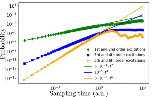
As a testbed for investigating the time-evolution of in Eq. (5), we consider the \ceH8 molecule. Since we take the Hartree-Fock state as the initial state , the notion of the order of electron excitations is naturally associated with each computational basis state . Because holds in Eq. (5) for states other than the Hartree-Fock state itself, grows as for small , where is the smallest integer satisfying . More simply speaking, grows as for small when is the -th order electron excitation (over the Hartree-Fock state), where () for even (odd) .
Figure 1 shows the average of for one/two-, three/four- and five/six-electron excitation states within the computational basis states having the largest probabilities at . The exact time evolution is considered in this figure. For small these obey the expected ,, and scaling, respectively. Deviation from this starts happening at around , where the series expansion in Eq. (5) is not so meaningful and many orders of the perturbations start to contribute to the probability .
IV.2 Performance of single-time TE-QSCI based on the Hartree-Fock state: exact and Trotterized time evolution
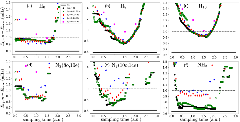
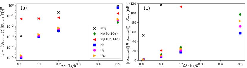
Here we investigate the performance of single-time TE-QSCI in detail from several points of view. Figure 2 shows the difference between the exact ground-state energy and the approximate energy obtained by single-time TE-QSCI as a function of the sampling time of the time-evolved state . We consider both exact time-evolution and first order Trotterization of the time-evolution operators with various step sizes . These results are based on the so-called statevector simulation of the quantum circuit where the effects of noise and sampling with a finite number of shots are not considered, so the computational basis states (or electron configurations) with largest amplitudes in are used to construct the subspace for the CI calculation. The dimension of the subspace is taken slightly larger than but much smaller than the dimension of the relevant sector of the Hilbert space. From this figure, we see that single-time QSCI can achieve sufficiently accurate results whose errors are below Hartree depending on the value of . A smaller Trotter step (or more accurate Trotterization of the time-evolution operator) results in a more accurate energy in general. The results also imply that an optimal range for the sampling time exists where the obtained energies are most accurate. Interestingly, the optimal time range is within for all the molecules studied here, despite large differences in the energy itself (e.g., the exact ground state energy is Hartree for \ceH6 and Hartree for \ceNH3).
Next, we analyze the required dimension of the subspace in the CI calculation of single-time TE-QSCI. The reference value for is that for GS-QSCI, , summarized in Table 1 at the beginning of this section and it allows us to evaluate the results of different molecules with a unified criterion. We present the energy difference between the exact energy and output of single-time TE-QSCI as a function of in Fig. 3, fixing the time at the optimal value. In general, TE-QSCI requires a larger than GS-QSCI but it also depends on the specific molecule; for example, it is rather small for \ceNH3 with small Trotter steps compared to the other 16 qubit examples. This is partially explained by the Hartree-Fock state of \ceNH3 having a large fidelity to the ground state . A more systematic investigation of the fidelity of the initial state to the exact ground state is presented in Appendix B.1. A second important observation in Fig. 3 is that an accurate energy below the error of Hartree can still be obtained for large Trotter steps (such as , which is large considering the evolution time is ), as long as we use a larger and pay the higher cost of the classical computation in the CI calculation. Note that \ceN2 and \ceNH3 molecules are more sensitive to the Trotter error than the hydrogen chains. This is possibly because of the smaller (and therefore in the plot) for these molecules, while the larger subspace required for the hydrogen chains can host the unnecessary bases due to the Trotter error and still give an accurate result. A more detailed investigation of the Trotter error in terms of the fidelity and energy conservation is presented in Appendix B.2.
So far, we have investigated single-time TE-QSCI based on the exact statevector simulation, but on real quantum hardware the time-evolved state will be sampled with a finite number of measurements. The measurements with a finite number of shots introduce the fluctuation of the measurement results of computational basis state, so the resulting output of TE-QSCI also fluctuates. In Fig. 4 we investigate the effect of a finite number of shots for a fixed at various values of the Trotter step size for the \ceH8, \ceN2(8o,10e), and \ceNH3 molecules. Contrary to the two previous figures in this subsection, the dimension of the subspace in this figure represents the number of all distinct computational bases (electron configurations) among measurement results. We run the simulation ten times to determine the sensitivity to the fluctuations of the measurement results, plotting the mean of the energy error to the exact energy as well as the sample standard deviation of the obtained energies. One can see from Fig. 4 that accurate energy is achievable even when considering the shot fluctuation of the measurement results with the standard deviation of the obtained energy being smaller than its mean by about an order of magnitude. The energy of single-time TE-QSCI is almost independent of the Trotter step size in this case, where we take all distinct electron configurations appearing in the measurement result to construct the subspace. This treatment results in larger at the same number of shots for the cases with larger Trotter steps since the larger Trotter error in the time evolution operator tends to generate a more “messy” state having a lot of small non-zero amplitudes. The large generally yields an accurate energy, compensating for the Trotter error with the drawback of a higher computational cost of the classical diagonalization.
Figures 3 and 4 suggest that it is possible to trade quantum resources for classical resources, i.e., even when using a less accurate Trotter approximation requiring a shallower circuit, the same accuracy can be obtained with the same number of measurements at the cost of having to diagonalize a larger matrix classically. This trade off is one of the interesting features of TE-QSCI although it is not desirable to push too far in this direction as the classical diagonalization is a major bottleneck for maximal feasible system sizes.
IV.3 Performance of time-average TE-QSCI
| Molecule | \ceH6 | \ceH8 | \ceN2(8o,10e) | \ceNH3 |
| at optimal time [mHa] | 0.93 | 0.78 | 0.86 | 0.70 |
| for infinite time average [mHa] | 2.01 | 1.78 | 2.86 | 1.34 |
| 90 | 850 | 130 | 100 |
| time [a.u.] | |||||
|---|---|---|---|---|---|
| [mHa] | 0.93 | 0.92 | 1.06 | 1.00 | 1.01 |
We investigate the performance of time-average QSCI in this subsection. First, in Table 2, we compare the accuracy of energy obtained for the infinite-time average calculated according to Eq. (7) with that of single-time TE-QSCI at the optimal time. The time evolution operator is simulated exactly without Trotterization, and the computational basis states (electron configurations) with the largest amplitudes are picked up to construct the subspace. The results in Table 2 indicate that the infinite-time-average TE-QSCI is not as accurate as single-time QSCI at the optimal time. GS-QSCI using the same can reach the precision of Hartree, but the infinite-time-average TE-QSCI is not equivalent to it because the overlap between the initial state and the exact ground state is not unity and the effect of other excited states is present.
However, we also find that time-average TE-QSCI can achieve accuracy competitive with single-time TE-QSCI at the optimal time depending on the choice of the time range for averaging. Table 3 presents the result of time-average TE-QSCI for various time ranges including the optimal time for the \ceH8 molecule. These results are based on the Trotterized time-evolution operator with . The time average is taken for by discretizing the range with . Concretely, we take for time-average TE-QSCI, where is the total number of times. In this case is chosen equal to the Trotter step size, but in general it can be larger than it. The shot simulation is employed and the total number of shots for measuring all times in the range is set to . The dimension of the subspace is taken as . The results in Table 3 illustrate that the performance of time-average TE-QSCI is comparable to single-time TE-QSCI at optimal time with the same number of shots and at the chosen time ranges. This observation is practically useful as we do not know the optimal time a priori, and this implies that accurate results can be obtained by averaging over times in a finite range.
IV.4 Comparing with UCCSD-QSCI based on classical CCSD amplitudes
| Molecule | \ceH6 | \ceH8 | \ceH10 | \ceN2(8o,10e) | \ceN2(10o,14e) | \ceNH3 |
| [mHa] | 0.389 | 1.073 | 1.980 | 4.517 | 4.518 | 0.210 |
| [mHa] | 0.924 | 1.464 | 2.114 | 2.101 | 2.053 | 0.633 |
| [mHa] | 0.970 | 0.983 | 0.997 | 0.974 | 0.972 | 0.984 |
| 87 | 781 | 5830 | 128 | 168 | 100 |
One of the advantages of TE-QSCI is avoiding the classical optimization of quantum circuits. In this part, we compare TE-QSCI with a similar approach to prepare an initial state of QSCI which also has this property.
Particularly, we consider the UCCSD ansatz [59] with Trotterization whose parameters are determined by the classical CCSD calculation. The UCCSD ansatz has been featured in applications of quantum computing to quantum chemistry and it can potentially express the approximate ground state by tuning its parameters. The definition of the UCCSD ansatz written in fermion operators we adopt in this study is as follows (implemented in the package Quri-Parts [60]:
| (9) | ||||
| (10) | ||||
| (11) | ||||
| (12) |
where is the Hartree-Fock state, () are the occupied (virtual) orbitals in the Hartree-Fock state, and are the circuit parameters. When implementing this as a quantum circuit, we transform the fermion operators in the exponentials into qubit operators using the Jordan-Wigner transformation and approximate those exponentials by Trotterization. The UCCSD ansatz is similar to the time evolution operator used in TE-QSCI except that it includes only the excitations from the occupied to virtual orbitals and its parameters must be tuned by some optimization. The optimization of the parameters are typically performed by expectation value estimation of the ansatz state, which requires a huge number of measurements in practice [7]. Nevertheless, it is suggested that the CCSD amplitudes obtained by the classical CCSD calculation are a good initial guess for the parameters [61]. Therefore, it is natural to use the UCCSD ansatz with the CCSD amplitudes as an input state of QSCI because such a state could have a large overlap with the exact ground state. We call QSCI with inputting the UCCSD ansatz with the CCSD amplitudes UCCSD-QSCI. It should be noted that the large-scale hardware experiment of QSCI [17] adopted a local version of the unitary cluster Jastrow ansatz [62, 63] which approximates the UCCSD ansatz with the CCSD amplitudes by the singular value decomposition of the CCSD amplitudes.
In Table 4, we compare the energy error of single-time TE-QSCI at the optimal time, UCCSD-QSCI and the classical CCSD calculation with respect to the exact ground state energy. Trotterization of five or seven steps is used for single-time TE-QSCI at the optimal time. The number of Trotter steps for the UCCSD ansatz is determined by monitoring the convergence of the output QSCI energy when increasing the number of steps. This gives only a single step for all molecules except for \ceH10 which needs twenty steps. The energy error obtained at the same dimension of the subspace is larger by UCCSD-QSCI than TE-QSCI for \ceH8, \ceH10 and \ceN2 while it is smaller for \ceH6 and \ceNH3. We summarize these results as follows: single-time TE-QSCI can outperform UCCSD-QSCI when the problems are large and/or more complicated and the CCSD calculation is not so accurate (the error is mHa). Therefore, for practical cases of interest, i.e., systems that do not allow for accurate CCSD energy, TE-QSCI may be useful to calculate the approximate ground-state energy. We note that the fidelity between the input state of QSCI and the exact ground state is larger for UCCSD-QSCI than TE-QSCI in general because the latter is just the overlap between the Hartree-Fock state and the exact ground state. In this sense it is interesting that TE-QSCI can outperform UCCSD-QSCI.
IV.5 System-size scaling of quantum and classical resources for TE-QSCI
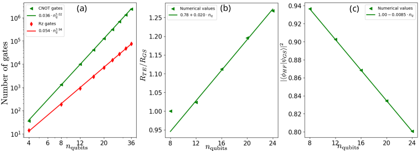
Finally, we investigate the system-size scaling of TE-QSCI focusing on its quantum and classical resources. This is important to tell whether our proposed method can tackle system sizes that cannot be exactly solved using classical methods. Specifically, we consider hydrogen chain molecules systematically increasing the number of hydrogen atoms or qubits. We construct the Hamiltonians [Eq. (2)] for \ceHn molecules where hydrogen atoms are aligned in a straight line with the atomic distance being 1 Åby using the Hartree-Fock orbital with the STO-3G basis set. The number of qubits for the Hamiltonian for the \ceHn molecule is .
As the basic quantum resource requirements of TE-QSCI, we estimated the number of elementary gates required to run the time-evolution operator (TEO) circuit once. The elementary gates considered in our estimation is the single qubit -rotation gate with arbitrary angle , the CNOT gate, and single-qubit Clifford gates. The number of CNOT gates is typically more important than that of single-qubit gates in the NISQ era because the fidelity of the former is much worse than the latter in currently available NISQ hardware. On the other hand, the number of rotation gates is crucial and that of CNOT becomes marginal when we have (early-)FTQC era in mind since the Clifford gates, including CNOT, are relatively easy to implement in FTQC and the non-Clifford gates such as are the most cost-consuming. To obtain a rough estimate of the number of these two gates for the TEO circuit in actual implementations, we consider the approximated TEO circuit which is Trotterized with a single step. The circuit consists of a sequence of the rotation gates by Pauli operators acting on qubits, and we decompose those rotation gates into CNOT gates and gates by the standard way [59]. Namely, when the weight of the Pauli operator, or the number of qubits on which the Pauli operator acts non-trivially, is , the rotation gate is decomposed into CNOT gates and one gate with other single-qubit Clifford gates. Note that this estimation assumes that all-to-all connectivity among qubits.
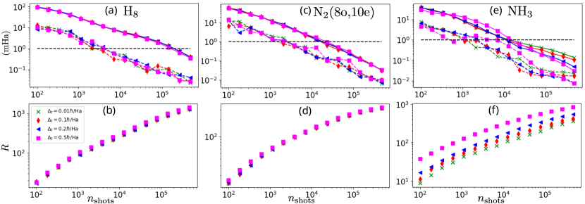
In Fig. 5(a), we show the numerical counts of the gates for implementing the TEO circuit with the single-step Trotterization (independent of the time of the TEO circuit). The counts obey a power law with the number of qubits, and the numerical fit gives the exponents as and . This is consistent with the generic expectation that the number of CNOT ( scales with () where is the number of qubits [59], explained by the fact that the TEO circuit (similar to the UCCSD anzats) has gates and each gate is decomposed into CNOTs and one gate on average. The number of CNOT gates for a single Trotter step is of the order of for the 36 qubit system where naive classical exact diagonalization becomes difficult. This count is rather large considering that the current quantum hardware often exhibits an error rate of for two-qubit gates, so performing TE-QSCI on NISQ devices for classically-intractable systems would need more improvement of the algorithm, quantum circuit, etc. On the other hand, the number of gates is on the order of for the 36 qubit system. This value is close to the maximal number of non-Clifford operations in the recently-proposed early-FTQC architecture called STAR [64], so TE-QSCI would be feasible on such devices. Note that we do not simplify the circuit, so there is much room for improving the estimate gate counts.
In addition to the number of elementary gates required for a single measurement, the total number of required measurements is another important aspect of the quantum resource estimation for practical applications. The number of required shots for GS-QSCI was discussed in the original proposal of QSCI [14] and generally it is comparable or smaller than the number of shots to estimate the Hamiltonian expectation value in the standard protocol once. This means that GS-QSCI is much more shot-efficient compared with other algorithms using the Hamiltonian expectation value, such as VQE or the quantum Krylov method. As we will show that TE-QSCI does not have large overhead compared with GS-QSCI, we expect that TE-QSCI also inherits the efficiency in the number of shots.
As the classical resource requirements for TE-QSCI, we investigate how the dimension of the subspace required to obtain accurate results scales with system size. Similarly to Sec. IV.2, we use the value of , which is defined such that GS-QSCI yields the sufficiently accurate ground-state energy whose error to the exact one is smaller than Hartree, as the reference to discuss for TE-QSCI. Note that the original proposal of QSCI [14] studied for hydrogen chains in detail. In Fig. 5(b), we show the ratio between the required for Hartree accuracy in single-time TE-QSCI at the optimal time () and GS-QSCI () as a function of the number of qubits. For a small system there is almost no added cost, but for there is a linear increase in the ratio with proportionality . The extrapolation to (50) leads to (1.78), so the additional classical computational cost of TE-QSCI compared with GS-QSCI using one of the optimal input states of QSCI is not so huge. One potential mechanism for the increase of the ratio is the decrease in the fidelity between the input state of TE-QSCI and the exact ground state, equivalent to the fidelity between the Hartree-Fock state and the exact ground state. The fidelity is shown in Fig.5(c) and it actually decrease linearly with . This may explain the increase of , but further investigation will be needed since the fidelity does not completely explain the performance of TE-QSCI (see also Appendix B.1).
V Summary, discussion and outlook
In this study, we have shown that applying the time-evolution operator to the Hartree-Fock state can generate promising candidate states for QSCI to calculate accurate ground-state energies of quantum chemistry Hamiltonians. We have investigated how the accuracy of this protocol, Time-Evolved QSCI (TE-QSCI), depends on the time, Trotter step size and the number of basis states in the selected subspace taking small molecules as examples. All investigated cases exhibit similar optimal time-ranges where the highest accuracy for single-time TE-QSCI is obtained when is kept fixed. Searching for the optimal time may require performing single-time TE-QSCI for multiple times and a large number of measurements, but time-average TE-QSCI is possibly useful to obtain the accurate energy without knowing the exact optimal time. In general, we also find that there is a trade-off between quantum and classical resources: increasing the Trotter step-size which reduces the number of gates in quantum circuits leads to more unimportant electron configurations in the selected subspace, but this can be compensated by increasing at the expense of a higher classical computational cost for exact diagonalization. We have compared the performance of TE-QSCI with a method potentially possessing a similar property, namely, UCCSD-QSCI where the UCCSD ansatz with the classically-calculated CCSD amplitudes is used as an input of QSCI. The numerical result indicates that when the classical CCSD calculation itself is inaccurate, TE-QSCI can give more accurate results than UCCSD-QSCI. Even using the exact time evolution and the optimal time, TE-QSCI has an intrinsic overhead in terms of the number of states required for a given accuracy in comparison with the number of states required when inputting the exact ground state to QSCI. Systematic analysis of the system-size scaling using the hydrogen chains represented by qubits revealed that the scaling of the overhead with the number of qubits was numerically found to be , suggesting that it is not prohibitive for practical application to large systems giving a value of, e.g., for 50 qubits. The scaling analysis on the number of quantum gates to implement the quantum circuit for TE-QSCI implies that the gates counts for classically-intractable problems is within the capability of early-FTQC devices such as that proposed in Ref. [64] though it seems difficult to run on current NISQ devices in the naive form. Overall, TE-QSCI can serve as a practical way to implement QSCI for calculating an accurate ground state without optimizing the quantum circuit by quantum-classical feedback or any particular knowledge of the ground state.
There are several interesting future directions of this study. First, it is vital to reduce the number of gates in Fig. 5(a) if we want to run TE-QSCI on actual NISQ hardware. For example, by relaxing the implementation of the time-evolution operator into a more approximated one than the Trotterization, like using the stochastic application of the gates [65] or dropping the gates depending on the hardware requirement [63, 17]. We stress that the estimation in Fig. 5(a) does not take any simplification of quantum circuits into account. Second, the main topic of investigation in this study was the time-evolved state from the Hartree-Fock state, but as shown in Appendix B.1 the accuracy of TE-QSCI can be improved by using different initial states. One idea is to run VQE or ADAPT-QSCI for a limited number of optimization steps, using the obtained circuit to prepare an initial state for TE-QSCI. Another straightforward idea which also avoids the optimization is to use the UCCSD ansatz with the CCSD amplitudes, investigated in Sec. IV.4, as the initial state of the time evolution of TE-QSCI. If the UCCSD circuit is implemented with Trotterization using a single step, additional gates required to use this initial state approximately corresponds to adding just a single time step to the time-evolution operator circuit as the UCCSD circuit has a similar form to the time-evolution operator. Third, as a related research direction, the application of QSCI to calculate the dynamics of quantum systems is important. By picking out important configurations at each time during the time-evolution by measuring the time-evolved state, we can construct a time-dependent subspace to be used for classical time-evolution methods.
Note added.
In the final stage of preparing this manuscript, Sugisaki et al. independently posted a manuscript to arXiv [18], which utilizes the same idea as this study and named their method the Hamiltonian-simulation based QSCI (HSB-QSCI). They considered the time-evolved states as inputs of QSCI and the dimension of the subspace was not fixed, whereas our proposal allows a more general framework and investigated the effect of limiting the maximum size of the subspace dimension. Their manuscript presents an interesting study focusing on the practical application to oligoacenes and includes an actual hardware experiment on IBM quantum devices. Our study has a different focus, namely investigating the optimality of the configurations chosen by TE-QSCI (or HSB-QSCI) in order to address how well the classical resource requirements of the method scales to large systems. We believe the two manuscripts are complimentary.
Acknowledgments
The authors thanks Keita Kanno for initiation of this research project and helpful discussion.
References
- Feynman [1982] R. P. Feynman, Simulating physics with computers, International Journal of Theoretical Physics 21, 467 (1982).
- Cao et al. [2019] Y. Cao, J. Romero, J. P. Olson, M. Degroote, P. D. Johnson, M. Kieferová, I. D. Kivlichan, T. Menke, B. Peropadre, N. P. D. Sawaya, S. Sim, L. Veis, and A. Aspuru-Guzik, Quantum chemistry in the age of quantum computing, Chemical Reviews 119, 10856 (2019).
- McArdle et al. [2020] S. McArdle, S. Endo, A. Aspuru-Guzik, S. C. Benjamin, and X. Yuan, Quantum computational chemistry, Rev. Mod. Phys. 92, 015003 (2020).
- Kitaev [1995] A. Y. Kitaev, Quantum measurements and the abelian stabilizer problem, arXiv preprint quant-ph/9511026 (1995).
- Cleve et al. [1998] R. Cleve, A. Ekert, C. Macchiavello, and M. Mosca, Quantum algorithms revisited, Proceedings of the Royal Society of London. Series A: Mathematical, Physical and Engineering Sciences 454, 339 (1998).
- Peruzzo et al. [2014] A. Peruzzo, J. McClean, P. Shadbolt, M.-H. Yung, X.-Q. Zhou, P. J. Love, A. Aspuru-Guzik, and J. L. O’Brien, A variational eigenvalue solver on a photonic quantum processor, Nature Communications 5, 4213 (2014).
- Tilly et al. [2022] J. Tilly, H. Chen, S. Cao, D. Picozzi, K. Setia, Y. Li, E. Grant, L. Wossnig, I. Rungger, G. H. Booth, and J. Tennyson, The variational quantum eigensolver: A review of methods and best practices, Physics Reports 986, 1 (2022).
- McClean et al. [2018] J. R. McClean, S. Boixo, V. N. Smelyanskiy, R. Babbush, and H. Neven, Barren plateaus in quantum neural network training landscapes, Nature Communications 9, 4812 (2018).
- Gonthier et al. [2022] J. F. Gonthier, M. D. Radin, C. Buda, E. J. Doskocil, C. M. Abuan, and J. Romero, Measurements as a roadblock to near-term practical quantum advantage in chemistry: Resource analysis, Phys. Rev. Res. 4, 033154 (2022).
- Layden et al. [2023] D. Layden, G. Mazzola, R. V. Mishmash, M. Motta, P. Wocjan, J.-S. Kim, and S. Sheldon, Quantum-enhanced markov chain monte carlo, Nature 619, 282 (2023).
- Huggins et al. [2022] W. J. Huggins, B. A. O’Gorman, N. C. Rubin, D. R. Reichman, R. Babbush, and J. Lee, Unbiasing fermionic quantum monte carlo with a quantum computer, Nature 603, 416 (2022).
- Parrish and McMahon [2019] R. M. Parrish and P. L. McMahon, Quantum filter diagonalization: Quantum eigendecomposition without full quantum phase estimation, arXiv preprint arXiv:1909.08925 (2019).
- Stair et al. [2020] N. H. Stair, R. Huang, and F. A. Evangelista, A multireference quantum krylov algorithm for strongly correlated electrons, Journal of Chemical Theory and Computation 16, 2236 (2020).
- Kanno et al. [2023] K. Kanno, M. Kohda, R. Imai, S. Koh, K. Mitarai, W. Mizukami, and Y. O. Nakagawa, Quantum-Selected Configuration Interaction: classical diagonalization of Hamiltonians in subspaces selected by quantum computers, arXiv preprint arXiv:2302.11320 (2023).
- Arute et al. [2019] F. Arute, K. Arya, R. Babbush, D. Bacon, J. C. Bardin, R. Barends, R. Biswas, S. Boixo, F. G. Brandao, D. A. Buell, et al., Quantum supremacy using a programmable superconducting processor, Nature 574, 505 (2019).
- Nakagawa et al. [2023] Y. O. Nakagawa, M. Kamoshita, W. Mizukami, S. Sudo, and Y.-y. Ohnishi, Adapt-qsci: Adaptive construction of input state for quantum-selected configuration interaction, arXiv preprint arXiv:2311.01105 (2023).
- Robledo-Moreno et al. [2024] J. Robledo-Moreno, M. Motta, H. Haas, A. Javadi-Abhari, P. Jurcevic, W. Kirby, S. Martiel, K. Sharma, S. Sharma, T. Shirakawa, I. Sitdikov, R.-Y. Sun, K. J. Sung, M. Takita, M. C. Tran, S. Yunoki, and A. Mezzacapo, Chemistry beyond exact solutions on a quantum-centric supercomputer (2024), arXiv:2405.05068 [quant-ph] .
- Sugisaki et al. [2024] K. Sugisaki, S. Kanno, T. Itoko, R. Sakuma, and N. Yamamoto, Hamiltonian simulation-based quantum-selected configuration interaction for large-scale electronic structure calculations with a quantum computer (2024), arXiv:2412.07218 [quant-ph] .
- Jordan and Wigner [1928] P. Jordan and E. Wigner, Über das paulische äquivalenzverbot, Zeitschrift für Physik 47, 631 (1928).
- Bravyi and Kitaev [2002] S. B. Bravyi and A. Y. Kitaev, Fermionic quantum computation, Annals of Physics 298, 210 (2002).
- Seeley et al. [2012] J. T. Seeley, M. J. Richard, and P. J. Love, The bravyi-kitaev transformation for quantum computation of electronic structure, The Journal of Chemical Physics 137, 224109 (2012).
- Helgaker et al. [2000] T. Helgaker, P. Jørgensen, and J. Olsen, Molecular Electronic-Structure Theory (John Wiley & Sons, 2000).
- Bender and Davidson [1969] C. F. Bender and E. R. Davidson, Studies in configuration interaction: The first-row diatomic hydrides, Physical Review 183, 23 (1969).
- Whitten and Hackmeyer [1969] J. Whitten and M. Hackmeyer, Configuration interaction studies of ground and excited states of polyatomic molecules. i. the ci formulation and studies of formaldehyde, The Journal of Chemical Physics 51, 5584 (1969).
- Huron et al. [1973] B. Huron, J. Malrieu, and P. Rancurel, Iterative perturbation calculations of ground and excited state energies from multiconfigurational zeroth-order wavefunctions, The Journal of Chemical Physics 58, 5745 (1973).
- Buenker and Peyerimhoff [1974] R. J. Buenker and S. D. Peyerimhoff, Individualized configuration selection in CI calculations with subsequent energy extrapolation, Theoretica chimica acta 35, 33 (1974).
- Buenker and Peyerimhoff [1975] R. J. Buenker and S. D. Peyerimhoff, Energy extrapolation in CI calculations, Theoretica chimica acta 39, 217 (1975).
- Nakatsuji [1983] H. Nakatsuji, Cluster expansion of the wavefunction, valence and rydberg excitations, ionizations, and inner-valence ionizations of CO2 and N2O studied by the sac and sac CI theories, Chemical Physics 75, 425 (1983).
- Cimiraglia and Persico [1987] R. Cimiraglia and M. Persico, Recent Advances in Multireference Second Order Perturbation CI: The CIPSI Method Revisited, J. Comput. Chem. 8, 39 (1987).
- Harrison [1991] R. J. Harrison, Approximating Full Configuration Interaction with Selected Configuration Interaction and Perturbation Theory, J. Chem. Phys. 94, 5021 (1991).
- Greer [1995] J. Greer, Estimating full configuration interaction limits from a Monte Carlo selection of the expansion space, The Journal of Chemical Physics 103, 1821 (1995).
- Greer [1998] J. Greer, Monte carlo configuration interaction, Journal of Computational Physics 146, 181 (1998).
- Evangelista [2014] F. A. Evangelista, Adaptive multiconfigurational wave functions, J. Chem. Phys. 140, 124114 (2014).
- Holmes et al. [2016a] A. A. Holmes, H. J. Changlani, and C. Umrigar, Efficient heat-bath sampling in Fock space, J. Chem. Theory Comput. 12, 1561 (2016a).
- Schriber and Evangelista [2016] J. B. Schriber and F. A. Evangelista, Communication: An adaptive configuration interaction approach for strongly correlated electrons with tunable accuracy, J. Chem. Phys. 144, 161106 (2016).
- Holmes et al. [2016b] A. A. Holmes, N. M. Tubman, and C. Umrigar, Heat-bath configuration interaction: An efficient selected configuration interaction algorithm inspired by heat-bath sampling, Journal of chemical theory and computation 12, 3674 (2016b).
- Tubman et al. [2016] N. M. Tubman, J. Lee, T. Y. Takeshita, M. Head-Gordon, and K. B. Whaley, A deterministic alternative to the full configuration interaction quantum Monte Carlo method, The Journal of chemical physics 145, 044112 (2016).
- Ohtsuka and Hasegawa [2017] Y. Ohtsuka and J. Hasegawa, Selected configuration interaction using sampled first-order corrections to wave functions, J. Chem. Phys. 147, 034102 (2017).
- Schriber and Evangelista [2017] J. B. Schriber and F. A. Evangelista, Adaptive configuration interaction for computing challenging electronic excited states with tunable accuracy, J. Chem. Theory Comput. 13, 5354 (2017).
- Sharma et al. [2017] S. Sharma, A. A. Holmes, G. Jeanmairet, A. Alavi, and C. J. Umrigar, Semistochastic heat-bath configuration interaction method: Selected configuration interaction with semistochastic perturbation theory, Journal of chemical theory and computation 13, 1595 (2017).
- Chakraborty et al. [2018] R. Chakraborty, P. Ghosh, and D. Ghosh, Evolutionary algorithm based configuration interaction approach, International Journal of Quantum Chemistry 118, e25509 (2018).
- Coe [2018] J. P. Coe, Machine learning configuration interaction, Journal of chemical theory and computation 14, 5739 (2018).
- Coe [2019] J. P. Coe, Machine learning configuration interaction for ab initio potential energy curves, Journal of chemical theory and computation 15, 6179 (2019).
- Abraham and Mayhall [2020] V. Abraham and N. J. Mayhall, Selected configuration interaction in a basis of cluster state tensor products, Journal of Chemical Theory and Computation 16, 6098 (2020).
- Tubman et al. [2020] N. M. Tubman, C. D. Freeman, D. S. Levine, D. Hait, M. Head-Gordon, and K. B. Whaley, Modern approaches to exact diagonalization and selected configuration interaction with the adaptive sampling CI method, Journal of chemical theory and computation 16, 2139 (2020).
- Zhang et al. [2020] N. Zhang, W. Liu, and M. R. Hoffmann, Iterative configuration interaction with selection, Journal of Chemical Theory and Computation 16, 2296 (2020).
- Zhang et al. [2021] N. Zhang, W. Liu, and M. R. Hoffmann, Further development of iCIPT2 for strongly correlated electrons, J. Chem. Theory Comput. 17, 949 (2021).
- Chilkuri and Neese [2021a] V. G. Chilkuri and F. Neese, Comparison of many-particle representations for selected-CI I: A tree based approach, Journal of Computational Chemistry 42, 982 (2021a).
- Chilkuri and Neese [2021b] V. G. Chilkuri and F. Neese, Comparison of many-particle representations for selected configuration interaction: II. Numerical benchmark calculations, Journal of Chemical Theory and Computation 17, 2868 (2021b).
- Goings et al. [2021] J. J. Goings, H. Hu, C. Yang, and X. Li, Reinforcement learning configuration interaction, Journal of chemical theory and computation 17, 5482 (2021).
- Pineda Flores [2021] S. D. Pineda Flores, Chembot: a machine learning approach to selective configuration interaction, Journal of Chemical Theory and Computation 17, 4028 (2021).
- Jeong et al. [2021] W. Jeong, C. A. Gaggioli, and L. Gagliardi, Active learning configuration interaction for excited-state calculations of polycyclic aromatic hydrocarbons, Journal of chemical theory and computation 17, 7518 (2021).
- Seth and Ghosh [2023] K. Seth and D. Ghosh, Active Learning Assisted MCCI to Target Spin States, Journal of Chemical Theory and Computation 19, 524 (2023).
- NIS [2022] NIST Computational Chemistry Comparison and Benchmark Database, NIST Standard Reference Database Number 101 (2022), release 22.
- Sun et al. [2018] Q. Sun, T. C. Berkelbach, N. S. Blunt, G. H. Booth, S. Guo, Z. Li, J. Liu, J. D. McClain, E. R. Sayfutyarova, S. Sharma, S. Wouters, and G. K.-L. Chan, Pyscf: the python-based simulations of chemistry framework, WIREs Computational Molecular Science 8, e1340 (2018).
- Sun et al. [2020] Q. Sun, X. Zhang, S. Banerjee, P. Bao, M. Barbry, N. S. Blunt, N. A. Bogdanov, G. H. Booth, J. Chen, Z.-H. Cui, J. J. Eriksen, Y. Gao, S. Guo, J. Hermann, M. R. Hermes, K. Koh, P. Koval, S. Lehtola, Z. Li, J. Liu, N. Mardirossian, J. D. McClain, M. Motta, B. Mussard, H. Q. Pham, A. Pulkin, W. Purwanto, P. J. Robinson, E. Ronca, E. R. Sayfutyarova, M. Scheurer, H. F. Schurkus, J. E. T. Smith, C. Sun, S.-N. Sun, S. Upadhyay, L. K. Wagner, X. Wang, A. White, J. D. Whitfield, M. J. Williamson, S. Wouters, J. Yang, J. M. Yu, T. Zhu, T. C. Berkelbach, S. Sharma, A. Y. Sokolov, and G. K.-L. Chan, Recent developments in the PySCF program package, The Journal of Chemical Physics 153, 024109 (2020).
- McClean et al. [2020] J. R. McClean, N. C. Rubin, K. J. Sung, I. D. Kivlichan, X. Bonet-Monroig, Y. Cao, C. Dai, E. S. Fried, C. Gidney, B. Gimby, P. Gokhale, T. Häner, T. Hardikar, V. Havlíček, O. Higgott, C. Huang, J. Izaac, Z. Jiang, X. Liu, S. McArdle, M. Neeley, T. O’Brien, B. O’Gorman, I. Ozfidan, M. D. Radin, J. Romero, N. P. D. Sawaya, B. Senjean, K. Setia, S. Sim, D. S. Steiger, M. Steudtner, Q. Sun, W. Sun, D. Wang, F. Zhang, and R. Babbush, Openfermion: the electronic structure package for quantum computers, Quantum Science and Technology 5, 034014 (2020).
- Suzuki et al. [2021] Y. Suzuki, Y. Kawase, Y. Masumura, Y. Hiraga, M. Nakadai, J. Chen, K. M. Nakanishi, K. Mitarai, R. Imai, S. Tamiya, T. Yamamoto, T. Yan, T. Kawakubo, Y. O. Nakagawa, Y. Ibe, Y. Zhang, H. Yamashita, H. Yoshimura, A. Hayashi, and K. Fujii, Qulacs: a fast and versatile quantum circuit simulator for research purpose, Quantum 5, 559 (2021).
- Anand et al. [2022] A. Anand, P. Schleich, S. Alperin-Lea, P. W. K. Jensen, S. Sim, M. Díaz-Tinoco, J. S. Kottmann, M. Degroote, A. F. Izmaylov, and A. Aspuru-Guzik, A quantum computing view on unitary coupled cluster theory, Chem. Soc. Rev. 51, 1659 (2022).
- qur [2022] QURI Parts (2022), https://github.com/QunaSys/quri-parts.
- Hirsbrunner et al. [2024] M. R. Hirsbrunner, D. Chamaki, J. W. Mullinax, and N. M. Tubman, Beyond MP2 initialization for unitary coupled cluster quantum circuits, Quantum 8, 1538 (2024).
- Matsuzawa and Kurashige [2020] Y. Matsuzawa and Y. Kurashige, Jastrow-type decomposition in quantum chemistry for low-depth quantum circuits, Journal of Chemical Theory and Computation 16, 944 (2020).
- Motta et al. [2023] M. Motta, K. J. Sung, K. B. Whaley, M. Head-Gordon, and J. Shee, Bridging physical intuition and hardware efficiency for correlated electronic states: the local unitary cluster jastrow ansatz for electronic structure, Chem. Sci. 14, 11213 (2023).
- Akahoshi et al. [2024] Y. Akahoshi, K. Maruyama, H. Oshima, S. Sato, and K. Fujii, Partially fault-tolerant quantum computing architecture with error-corrected clifford gates and space-time efficient analog rotations, PRX Quantum 5, 010337 (2024).
- Campbell [2019] E. Campbell, Random compiler for fast hamiltonian simulation, Phys. Rev. Lett. 123, 070503 (2019).
Appendix A Series expansion for time-dependent probability
We present the derivation of Eq. (5) in the main text.
We consider the series expansion which leads to
| (13) |
Let us consider the terms where or separately. Defining and considering or gives and , respectively, so we can gather these two terms in one by taking two times the real value. The special case of leads to , so overall this part of the double-sum can be expressed as
| (14) |
The remaining terms are
| (15) |
We then consider the case where and separately. For the sum straightforwardly gives
| (16) |
For the latter we can rewrite the sum as two times the real part, restricting the sum to values which gives
| (17) |
This sum can be given a more useful schematic form by substituting with the index where , leading to
| (18) |
We can then relabel all as , which leads to Eq. (5) in the main text when putting all terms together.
Appendix B Supplementary numerical results
B.1 Dependence of TE-QSCI on the input state and bond distance for 16 qubit hydrogen chain
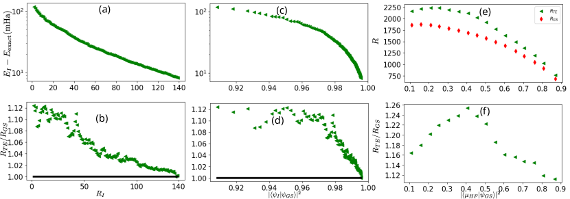
In this section, we study the accuracy dependence on the fidelity between the initial state of the time evolution of single-time TE-QSCI and the exact ground state, using the 16 qubit hydrogen chain \ceH8 as an example. We systematically change the fidelity of the initial state in two ways. The first one uses an artificial input state obtained by classical calculation while the Hamiltonian is fixed. The second one, on the contrary, keeps the initial state as the Hartree-Fock state and varies the Hamiltonian. We stress that the fidelity between the time-evolved state and the exact ground state is constant during the time evolution, so the initial state of the time evolution solely determines the fidelity. As in Sec. IV.5 we denote the smallest dimension of the subspace required to obtain Hartree accuracy for single-time TE-QSCI at the optimal time and GS-QSCI as and , respectively.
Let us explain the first approach and its result. We prepare the initial state of the time evolution by choosing computational basis states (electron configurations) using the amplitudes of the exact ground state, sorted in descending order. Classical exact diagonalization in the -dimensional subspace is performed and the resulting lowest-energy eigenstate is employed as the input for the time evolution. We can vary the fidelity of the initial state by changing the value of . Figure 6(a)-(d) shows the lowest energy in the -dimensional subspace and . As expected, when becomes large and the fidelity between the initial state and the exact ground state gets close to unity, the ratio becomes smaller. Note that even for the data points close to the fidelity , the value of is much smaller than , leading to Hartree. This means the value of indicating that results are on par with GS-QSCI is due to TE-QSCI generating important configurations not present in the initial state.
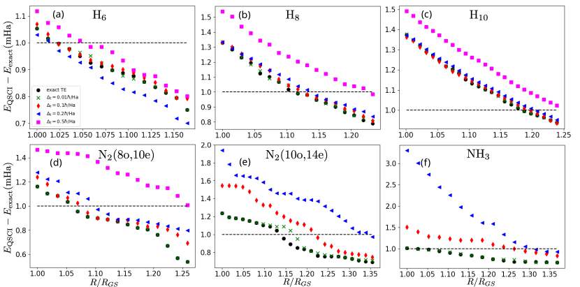
The second approach we take to vary the fidelity of the initial state is increasing the bond length (atomic distance) of \ceH8 from the original value of Å. Because the Hartree-Fock state becomes a worse approximation of the ground state for larger bond lengths, the fidelity correspondingly decreases. In Fig. 6(e,f) we plot , and , respectively, for different bond lengths between Å and Å as a function of , where () is the Hartree-Fock state (exact ground state). Interestingly, in this case the ratio is not monotonically decreasing with the fidelity. It is also surprising that single-time QSCI can give an accurate energy with relatively small additional classical computational resources () despite the small fidelity.
In short, the results in this section suggest that while a large fidelity between the initial state of the time evolution and the exact ground state saves classical computational cost (small ), it is not the sole factor determining the performance of single-time TE-QSCI.
B.2 Fidelity and the energy conservation of the Trotterized time evolution
In Sec. IV.2, it was seen that single-time TE-QSCI is relatively robust towards the Trotter error for hydrogen chains while it is somewhat less robust for \ceN2 and \ceNH3. In this section, we present more detailed data of the error associated with the Trotterized time evolution, finding the same overall trend. In Fig. 7, we plot the infidelity between the state after the Trotterized time-evolution and the exact time-evolved state, as well as the violation of the energy conservation during the time evolution , at the optimal times corresponding to Fig. 3. An observed overall tendency is that the hydrogen chains exhibit smaller values both for the infidelity and the violation of the energy conservation than \ceN2 and \ceNH3, which may result in the accurate output energy of single-time TE-QSCI seen in Fig. 2. Although it is hard to make any strong conclusions based on these results, the accuracy of single-time TE-QSCI generally get worse if both the infidelity and energy error are large. Moreover, it is interesting and promising that single-time TE-QSCI can give the accurate energy error of Hartree even when the Trotter error measured by the violation of the energy conversation is much larger than it.