Nullu: Mitigating Object Hallucinations in Large Vision-Language Models via HalluSpace Projection

Abstract

Recent studies have shown that large vision-language models (LVLMs) often suffer from the issue of object hallucinations (OH). To mitigate this issue, we introduce an efficient method that edits the model weights based on an unsafe subspace, which we call HalluSpace in this paper. With truthful and hallucinated text prompts accompanying the visual content as inputs, the HalluSpace can be identified by extracting the hallucinated embedding features and removing the truthful representations in LVLMs. By orthogonalizing the model weights, input features will be projected into the Null space of the HalluSpace to reduce OH, based on which we name our method Nullu. We reveal that HalluSpaces generally contain statistical bias and unimodal priors of the large language models (LLMs) applied to build LVLMs, which have been shown as essential causes of OH in previous studies. Therefore, null space projection suppresses the LLMs’ priors to filter out the hallucinated features, resulting in contextually accurate outputs. Experiments show that our method can effectively mitigate OH across different LVLM families without extra inference costs and also show strong performance in general LVLM benchmarks. Code is released at https://github.com/Ziwei-Zheng/Nullu.

1 Introduction

Recent advancements in large language models (LLMs) [1, 40, 35] have spurred rapid developments in large vision-language models (LVLMs), such as GPT-4V [1], Gemini [39], LLaVA [31] and mPLUG-Owl2 [48]. By integrating a vision encoder and fine-tuning on multimodal instruction-following datasets, LVLMs exhibit a strong ability to interpret and convert complex visual patterns into coherent linguistic representations. Whereas, the widespread use of these LVLMs has shed light on their limitations—object hallucinations (OH).

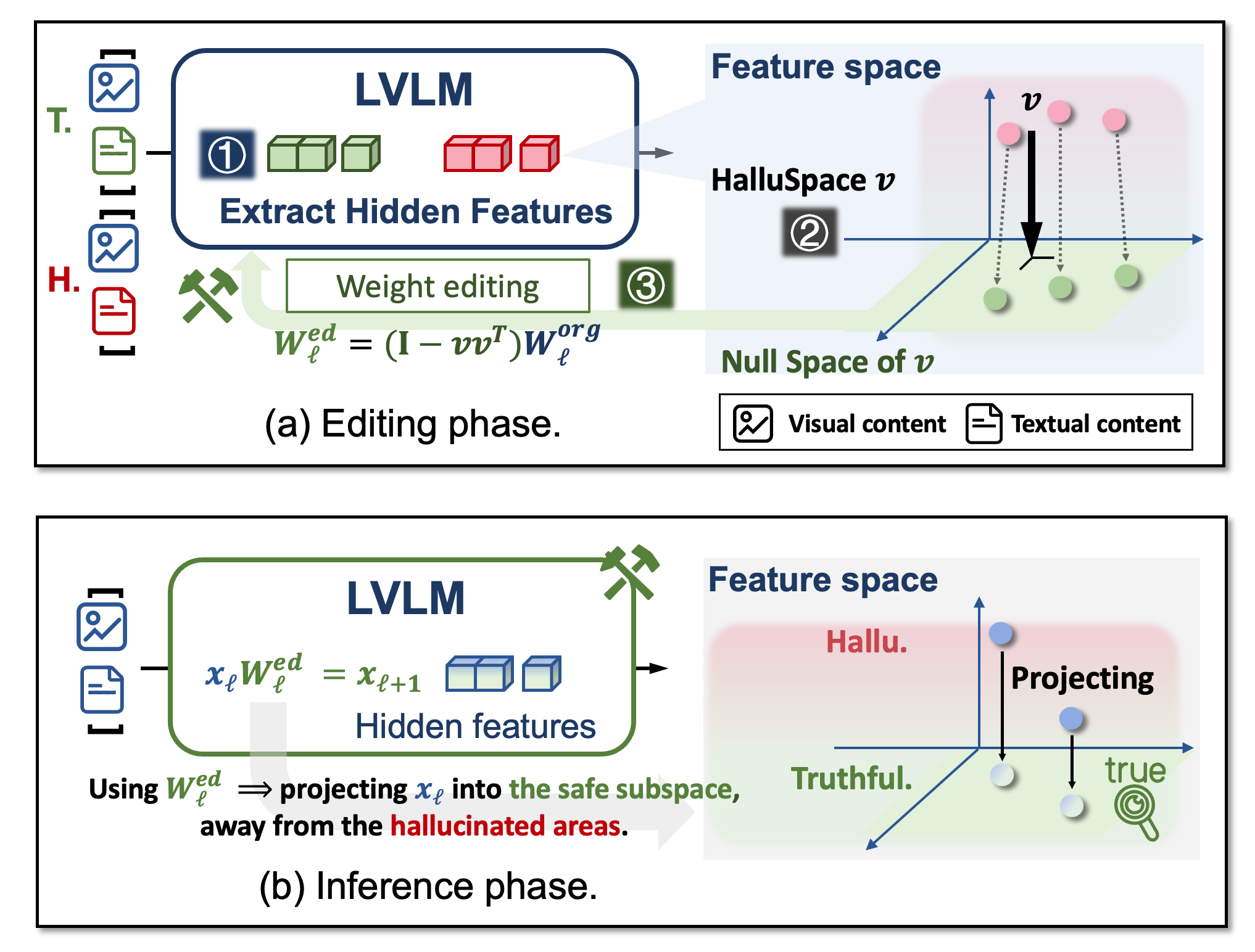
Figure 1: An illustration of Nullu. (a) In the editing phase, Nullu will ① Extract hidden features of truthful (T.) and hallucinated (H.) inputs. ② Explore a low-rank HalluSpace ${\bm{v}}$ in the feature space by contrasting the differences between T. and H. features. ③ Edit the model weights by projecting them to the null space of ${\bm{v}}$. (b) In the inference phase, using the edited weights equals to project input features into the safe subspace, away from the hallucinated areas, leading to contextually accurate outputs.

Object Hallucination (OH) refers to the phenomenon where LVLMs generate text that, while semantically coherent, inaccurately represents the actual objects in the accompanying image [29, 4, 20, 24, 27]. Considering the wide application of LVLMs in different fields like autonomous driving [34] and embodied AI [23], hallucinations in generated content can lead to misinformation or even harmful decisions. Therefore, mitigating OH is crucial for AI safety and trustworthiness. Recent works propose to address OH by either performing fine-tuning in an end-to-end manner [29, 20, 22] or using post-processing methods to modify model outputs [24, 50, 53, 9], which show effectiveness in mitigating OH for modern open-source LVLMs.

Despite significant efforts, the underlying causes of OH within the models remain unexplored. This study investigates this issue by systematically examining the intrinsic distinctions between truthful and hallucinated responses, focusing on feature spaces. Our empirical results on open-source LVLMs reveal a low-rank subspace in the model parameter space, which we term “HalluSpace”, representing the distinction between truthful and untruthful feature distributions, and can be a factor triggering OH.

Building on this finding, we propose to mitigate OH by projecting away the detected HalluSpaces at each layer of LVLMs. Namely, we project the original model weights to the null space of HalluSpaces, based on which we build a novel method called Nullu. The framework of Nullu is shown in Figure 1. Our method first applies Principal Component Analysis (PCA) to extract the low-dimensional subspaces (HalluSpaces) from the difference matrix between truthful and hallucinated features at different layers. Then, by orthogonalizing model weights with respect to the HalluSpaces, Nullu effectively nullifies OH representations for any input, filtering out these untruthful features and resulting in contextually more accurate outputs.

By decoding the HalluSpace, we found that these subspaces are closely tied to statistical bias and unimodal priors of the LLMs applied to build LVLMs, shown to be primary causative factors of OH [24, 50]. Therefore, projecting model weights to the null space of HalluSpace offers a distinct but straightforward approach to reducing these biases. Furthermore, we establish theoretical connections between Nullu and Direct Preference Optimization (DPO) [36], showing that both of these two methods attempt to achieve a similar goal to avoid OH.

Through comprehensive experiments, we demonstrate the effectiveness of Nullu in mitigating OH without compromising the models’ general performance. Notably, Nullu needs no additional fine-tuning procedure and, introduces no extra inference costs compared to most post-hoc based methods [9, 24, 50], making Nullu much more efficient in alleviating OH. Our main contributions are as follows:

1. We propose a novel method named Nullu, which explores a new distinct strategy for OH mitigation. By extracting HalluSpaces and orthogonalizing the model weights, Nullu can effectively mitigate OH with no extra inference cost. Our method demonstrates the feasibility and effectiveness of mitigating OH by editing weight based on representation learning.

2. We uncover and show that HalluSpaces appear to form a prior closely related to the inherent biases of LLMs. Therefore, the HalluSpace Projection coincides with previous studies debiasing LVLMs to reduce OH at outputs. Moreover, our theoretical analysis shows the connection between Nullu and DPO. We hope our work can provide nuanced insights, broadening the understanding of potential causes behind unsafe behaviors within LVLMs.

3. Experiments show that using Nullu achieves consistent improvements with zero-extra costs on the evaluated tasks across different LVLMs, including LLAVA-1.5 [30], MiniGPT-4 [54], and mPLUG-Owl2 [48], demonstrating the effectiveness and efficiency of Nullu.

2 Related Work

2.1 Large Visual-Language Models (LVLMs)

Based on the development of LLMs, such as LLaMA [41] and Vicuna [10], large vision-language models (LVLMs) have made significant advancements in recent years. Early works, such as BLIP [25, 26] and BERT-based VLMs [12, 33], have successfully adapted LLMs to visual tasks, demonstrating notable generative capabilities and in-context learning abilities. These advancements typically involve connecting a vision encoder to an LLM through various fused modules, such as linear projection [31] or a Q-former [54]. With the adoption of visual instruction tuning techniques, LVLMs [31, 52] have further enhanced their abilities, enabling language generation models to perform complex image understanding and reasoning tasks, resulting in a series of modern well-performed LVLMs, such as LLaVA [31, 30], Mini-GPT4 [54], mPLUG-Owl [48, 47], Shikra [6], InternVL [8] and Qwen-VL [2, 3]. However, despite these successes, recent LLMs and LVLMs still face security issues [43, 51, 21], such as hallucination [4],

2.2 Mitigation of Object Hallucination

In LVLMs, object hallucination occurs when the model generates semantically coherent texts misaligned with actual objects in the accompanying image [37, 46, 45, 19]. Various approaches have been proposed to address this issue. Considering a possible cause of hallucination lies in data biases and the knowledge gap between visual and linguistic information, recent studies propose to fine-tune the LVLMs for robustness [29, 17], cross-modality matching [20, 22] or preference alignments [38, 7]. While these methods are effective, they are notorious for the demands of substantial computational resources for training and fine-tuning.

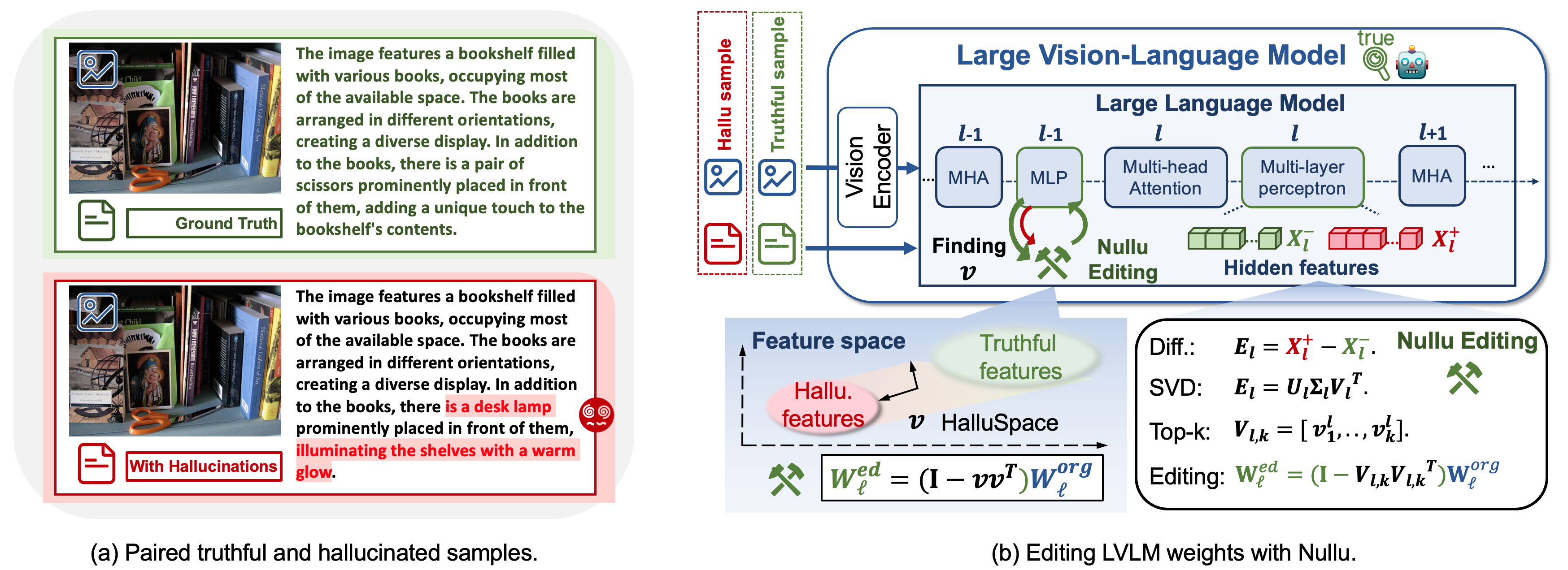
Figure 2: An overview of Nullu, which identifies the HalluSpaces to edit model weights for LVLMs. (a) The paired truthful and hallucinated samples. (b) Nullu first calculates the difference matrix of hidden features for the paired samples and then conducts the SVD to find the main directions of the difference as the HalluSpace. Then Nullu projects the original MLP’s weights to the null space of the HalluSpace. This procedure will be repeated for a series of layers, $\{\ell\}$, in the LLM of an LVLM.

To avoid high computational costs for training, recent studies also propose post-processing methods to mitigate OH, which apply new strategies or external tools to modify the response. LURE [53] trains a reviser to edit the possible hallucinated words in the responses. There is also a line of research that incorporates an external visual model to review entities extracted from the response, with the detection outcomes subsequently passed to the generation model to produce improved answers [49, 5, 9]. Moreover, recent studies have revealed that the LVLMs are often affected by the strong LLM’s prior during outputting, and visual uncertainty increases hallucination descriptions, leading to less attention to the visual contexts and resulting in OH [24, 32, 50, 55, 18, 13].

Despite these efforts, the underlying causes of OH within the models are still under investigation, which motivates this paper. Our work reveals that by contrasting the truthful and hallucinated features, Nullu can effectively eliminate the LLMs prior based on the learned HalluSpaces. Compared to post-processing methods like HALC [9] and VCD [24], our method does not introduce extra inference costs or additional models as assistance, demonstrating the efficiency of our method in OH mitigation.

3 Method

The framework of Nullu is illustrated in Figure 2. We first describe how to construct the data pairs of truthful and hallucinated text prompts, then introduce how Nullu extracts the HalluSpace to edit the model weights. We further provide an in-depth analysis by decoding the HalluSpaces, and discuss the connection between Nullu and DPO.

3.1 Data-pair construction

We begin with constructing paired vision-language inputs as shown in Figure 2 (a). The two inputs have the same image but different text prompts, where one contains the truthful ground truth, $x_{i}^{-}$, that accurately describes the objects in the image, and the other contains hallucinated descriptions, $x_{i}^{+}$. The whole dataset can be represented by $\mathcal{D}={(x_{i}^{+},x_{i}^{-})}_{i=1}^{N}$.

As it is stated in [53], the hallucinatory descriptions can be generated by modifying the accurate descriptions using GPT-3.5. These adjustments are guided by factors related to object hallucination, including co-occurrence, object uncertainty, and object position. Moreover, the hallucinatory descriptions can also been generated using the language bias based responses by distorting the visual inputs as in [24].

3.2 Nullu

Exploring HalluSpaces.

At each model layer $\ell$ in the LLM of the LVLM, where $\ell\in{L_{0}\dots L}$, we compute embedding features, denoted as ${\bm{x}}_{i,\ell}^{+}$ and ${\bm{x}}_{i,\ell}^{-}$ for the truthful and hallucinated features, respectively. We then average each sample at the token dimension and stack these embedding features into matrices ${\bm{X}}_{\ell}^{+}$, ${\bm{X}}_{\ell}^{-}\in\mathbb{R}^{N\times D}$, where $D$ is the embedding dimension. Then the difference matrix ${\bm{E}}_{\ell}$ at $\ell$-th layer can be calculated by:

$${\bm{E}}_{\ell}={\bm{X}}_{\ell}^{+}-{\bm{X}}_{\ell}^{-}\;,\;\;{\bm{E}}_{\ell}\in\mathbb{R}^{N\times D}.$$ (1)

We conduct the principal component analysis for ${\bm{E}}_{\ell}$ via singular value decomposition (SVD). As shown in Figure 2 (b), this matrix contains the underlying differences between the truthful and hallucinated embeddings in the feature space. Therefore, by exploring the structure of ${\bm{E}}_{\ell}$, we can find the main directions as a low-rank approximation of ${\bm{E}}_{\ell}$, based on which we can effectively eliminate the hallucinated features. Formally, the SVD can be conducted by

$${\bm{E}}_{\ell}={\bm{U}}_{\ell}\mathbf{\Sigma}_{\ell}{\bm{V}}_{\ell}^{\top},\;{\bm{U}}_{\ell}\in\mathbb{R}^{N\times N},\;{\bm{V}}_{\ell}\in\mathbb{R}^{D\times D},$$ (2)

where $\mathbf{\Sigma}_{\ell}$ is the diagonal matrix containing the singular values with the descending sort.

Next, we pick the right singular vectors with top-$k$ singular values, ${\bm{v}}_{1}^{\ell},{\bm{v}}_{2}^{\ell},\ldots,{\bm{v}}_{k}^{\ell}$, which are the first $k$ column vectors of ${\bm{V}}_{\ell}$. These directions represent the main difference between the truthful and hallucinated features and, therefore, can be considered the directions in model weight spaces that trigger the hallucinated descriptions. Therefore ${\bm{V}}_{\ell,k}=[{\bm{v}}_{1},...,{\bm{v}}_{k}]\in\mathbb{R}^{D\times k}$ is the target HalluSpace.

Usually, with a $k\ll D$, the HalluSpace can be well defined, which means the hallucinated descriptions are possible within a low-rank dimensionality. We then show how to edit the model weights to mitigate OH in LVLMs.

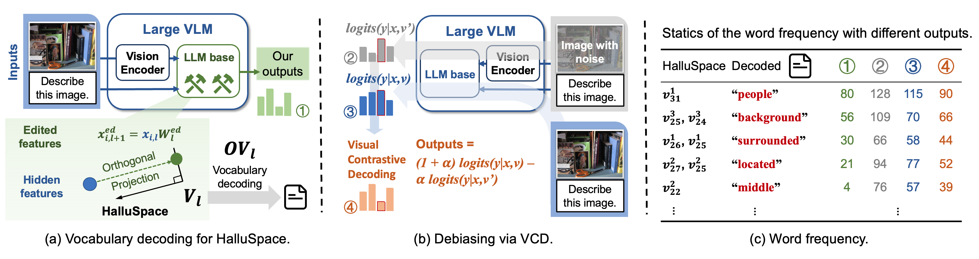
Figure 3: The relation between Nullu and methods for mitigating OH via debiasing [24, 50]. (a) The inference procedure of ours. (b) The inference procedure of VCD [24]. (c) The statics of the word frequency with different outputs.

Editing the model weights.

As the ${\bm{V}}_{\ell,k}$ represents the main different directions between the truthful and untruthful data distributions, we can effectively remove the hallucination information from the model features by projecting them to the null space of HalluSpace. As all inputs share this null space, we can directly orthogonalize the model weights with respect to ${\bm{V}}_{\ell,k}$. The null space of ${\bm{V}}_{\ell,k}$ can be presented by $({\bm{I}}-{\bm{V}}_{\ell,k}{\bm{V}}_{\ell,k}^{\top})$.

Therefore, we project the original weights of MLP at $\ell$-th layer ${\bm{W}}_{\ell}^{\text{org}}$ to the null-space of ${\bm{V}}_{\ell,k}$ with

$${\bm{W}}_{\ell}^{\text{ed}}=({\bm{I}}-{\bm{V}}_{\ell,k}{\bm{V}}_{\ell,k}^{\top})\;{\bm{W}}_{\ell}^{\text{org}}\;.$$ (3)

With the ${\bm{W}}_{\ell}^{\text{ed}}$, Nullu can effectively mitigate OH while generating responses. Moreover, as the new weights can be directly loaded into the model, there is no extra cost during inference, making our method more efficient compared to many existing methods.

Nullu.

Combining all components, we summarize Nullu in Algorithm 1. Our method contains two key parameters: the indices of layers needed to be editing $\{\ell\}$ and the selected top-$k$ singular vectors. Although we do not have a theoretical argument for the best values, we explore their effects experimentally and determine optimal values via a standard hyper-parameter sweep.

Algorithm 1 Nullu

Input: Paired data $\mathcal{D}$, LVLM $\mathcal{M}$, target layers $\{\ell\}$, rank number $k$.

Output: Edited LVLM $\mathcal{M}^{ed}$.

for $\ell$ in $\{\ell\}$ do

     Calculating ${\bm{X}}_{\ell}^{+}$ and ${\bm{X}}_{\ell}^{-}$ $\triangleright$ Hidden features

     ${\bm{E}}_{\ell}={\bm{X}}_{\ell}^{+}-{\bm{X}}_{\ell}^{-}$

     ${\bm{E}}_{\ell}={\bm{U}}_{\ell}\mathbf{\Sigma}_{\ell}{\bm{V}}_{\ell}^{\top}$

     ${\bm{V}}_{\ell,k}=[{\bm{v}}_{1},...,{\bm{v}}_{k}]$ $\triangleright$ Selecting Top-$k$

     ${\bm{W}}_{\ell}^{\text{ed}}=({\bm{I}}-{\bm{V}}_{\ell,k}{\bm{V}}_{\ell,k}^{\top})\;{\bm{W}}_{\ell}^{\text{org}}$ $\triangleright$ Editing $\ell$-th MLP

end for

3.3 Decoding information in HalluSpace

This subsection provides a case study to explore how the proposed Nullu mitigates OH. We conduct the analysis experiments on CHAIR [37] with LURE [53], which provides the ground truth and possible hallucinated responses with each visual input. The introduction of the dataset is provided in Section 4. We use LLaVA-1.5-7B [30] for our evaluation.

Mapping the subspace back to vocabulary.

Following previous works [16, 42], to explore the information behind the learned vectors ${\bm{v}}_{i}\in\mathbb{R}^{D}$, a common approach is to decode the embeddings with ${\bm{O}}{\bm{v}}\in\mathbb{R}^{|\mathcal{V}|}$, where ${\bm{O}}=[{\bm{o}}_{1},\ldots,{\bm{o}}_{|\mathcal{V}|}]^{\top}\in\mathbb{R}^{|\mathcal{V}|\times D}$ and $\mathcal{V}$ denotes the vocabulary. We then sort ${\bm{O}}{\bm{v}}$ in ascending order, find the top-$m$ indices, and use the corresponding words to interpret ${\bm{v}}$. The following analysis is performed at each layer $\ell$, while we will drop $\ell$ to avoid the notational burden.

Using Nullu, we can extract the ${\bm{V}}$ at different layers and then decode it via ${\bm{O}}{\bm{v}}$ to explore the internal information behind ${\bm{V}}$. For better interpretation, we only select the most representative results, shown in Figure 3 (c). As far we know, by projecting the model weights to the orthogonal direction of ${\bm{V}}$, Nullu can reduce the semantic information of the decoded words during responding. However, why does such a procedure mitigate OH?

Debiasing LVLM from LLM prior.

Recent studies [24, 50, 55, 32, 18] have revealed that hallucinated responses of LVLMs can be attributed to the strong LLMs’ prior. Therefore, following the settings in [24], we collect the outputs of LLaVA-1.5 with normal inputs and visually distorted inputs, as shown in Figure 3 (b). The static results of word frequency of ② and ③ show that LLMs indeed bias on some words during output generation. Therefore, modern techniques proposed to calibrate the outputs by reducing these detected LLM biased information [24, 50], or, in the opposite, enhancing the visual information [55, 32, 18] during inference. This can be confirmed by the word frequency results of ④. (See more results in Supplementary materials.)

Interpreting HalluSpace.

From the results in Figure 3 (b), ①, and the complete results in Supplementary materials, we see that the decoded words from HalluSpace are with high frequency when with the distorted visual inputs, indicating that HalluSpace ${\bm{V}}$ contains the similar abstract latent information as LLM’s prior does. Moreover, by visual contrastive decoding, we see that these LLM’s “preferred” words are reduced, corresponding to the results of Nullu. Therefore, we further indicate that Nullu projects the features to the null space of the HalluSpace ${\bm{V}}$, achieving a similar function of reducing LLM prior in LVLMs. By editing the LVLMs with Nullu the lower CHAIR_S (the metric to evaluate hallucination, the lower, the better) indicates that OH is effectively mitigated by Nullu. Therefore, we can consider Nullu as a new way that achieves debiasing from the model parameter aspect.

3.4 Theoretical Analysis: How Nullu works?

The analysis is performed for each layer $\ell$, and to avoid the notational burden, we will drop $\ell$ and focus on each layer separately. We also suppose the number of tokens as 1; the generated features can then be calculated as ${\bm{f}}_{i}={\bm{x}}_{i}{\bm{W}}^{\text{org}}$, where ${\bm{W}}^{\text{org}}\in\mathbb{R}^{D\times D_{o}}$, and ${\bm{x}}_{i}\in\mathbb{R}^{1\times D}$, ${\bm{f}}_{i}\in\mathbb{R}^{1\times D_{o}}$.

Based on the heuristic in [42], an embedding vector in any transformer layer can be decomposed into interpretable components. We suppose that the generated features ${\bm{f}}_{i}$ can be separated into three different elements:

$${\bm{f}}_{i}\Rightarrow\underbrace{\hat{\bm{f}}_{i}\hat{\bm{B}}}_{\text{truthful contexts}}+\underbrace{\widetilde{\bm{f}}_{i}\widetilde{\bm{B}}}_{\text{hallucinated biases}}+\underbrace{{\bm{u}}_{i}}_{\text{noise}},$$ (4)

where we suppose $\hat{\bm{B}}\in\mathbb{R}^{\hat{k}\times D_{o}}$ contains the truthful directions and $\widetilde{\bm{B}}\in\mathbb{R}^{\widetilde{k}\times D_{o}}$ contains $\widetilde{k}$ hallucinated directions, and ${\bm{u}}_{i}$ represents typical randomness unaccounted for by the statistical model. $\hat{\bm{f}}_{i}\in\mathbb{R}^{1\times\hat{k}},\widetilde{\bm{f}}_{i}\in\mathbb{R}^{1\times\widetilde{k}}$ are “latent factors”. Therefore $\widetilde{\bm{f}}_{i}\widetilde{\bm{B}}$ can represent the hallucinated features for the $i$-th input.

However, with the edited model weights ${\bm{W}}^{\text{ed}}$ using Eq. (3) and combining the hypothesize in Eq. (11), the edited features can be calculated as

$${\bm{f}}_{i}^{\text{ed}} ={\bm{x}}_{i}({\bm{I}}-{\bm{V}}_{k}{\bm{V}}_{k}^{\top}){\bm{W}}^{\text{org}}$$

$$=\hat{\bm{f}}_{i}\hat{\bm{B}}+(\widetilde{\bm{f}}_{i}\widetilde{\bm{B}}-({\bm{x}}_{i}{\bm{V}}_{k})({\bm{V}}_{k}^{\top}{\bm{W}}^{\text{org}}))+{\bm{u}}_{i}.$$ (5)

As the ${\bm{V}}_{k}$ gives the best rank-$k$ principle component approximation of the difference between the truthful and untruthful features via SVD, our approach can remove these hallucinated features and enhance the truthful answers to achieve more reliable responses.

Relation to DPO

Following previous studies in [42], we exhibit the conceptual connection between DPO [36] and Nullu by studying a simple logistic model $\pi_{{\bm{W}}}$ for the output given ${\bm{x}}$ as inputs. The conditional probability can be

$$\pi_{{\bm{W}}}(y|{\bm{x}}_{i})=Z_{{\bm{W}}}^{-1}\exp\big{(}{\bm{o}}_{y}^{\top}{\bm{W}}{\bm{x}}_{i}\big{)}$$ (6)

where ${\bm{o}}_{y}$ is the output decoding vector for any $y\in\mathcal{V}$, $Z_{{\bm{W}}}$ is the normalization factor. Similar expression holds for ${\bm{x}}_{i}^{+}$ and ${\bm{x}}_{i}^{-}$. With some calculations, the gradient with respect to ${\bm{W}}$ of the DPO loss can be represented as

$$\nabla_{{\bm{W}}}\mathcal{L}_{\text{DPO}}=-\frac{\beta}{N}\sum_{i=1}^{N}\big{(}{\bm{o}}_{y_{i}^{+}}({\bm{x}}_{i}^{+})^{\top}-{\bm{o}}_{y_{i}^{-}}({\bm{x}}_{i}^{-})^{\top}\big{)}$$

$$= -\frac{\beta}{N}\sum_{i=1}^{N}\big{(}\underbrace{{\bm{o}}_{y_{i}^{+}}({\bm{x}}_{i}^{+}-{\bm{x}}_{i}^{-})^{\top}}_{\text{feature difference}}+\underbrace{({\bm{o}}_{y_{i}^{+}}-{\bm{o}}_{y_{i}^{-}})({\bm{x}}_{i}^{-})^{\top}}_{\text{output difference}}\big{)}.$$ (7)

The gradient in (3.4) contains a feature difference term. Therefore, the gradient update can be interpreted as an attempt to eliminate feature differences to avoid hallucinated responses. For Nullu, it tries to approximate such difference via SVD and also attempts to eliminate it by null space projection, which shows the connection between Nullu and DPO. See Supplementary Materials for more details.

Method	LLaVA-1.5			MiniGPT-4			mPLUG-Owl2
	CHAIR${}_{S}\downarrow$	CHAIR${}_{I}\downarrow$	BLEU$\uparrow$	CHAIR${}_{S}\downarrow$	CHAIR${}_{I}\downarrow$	BLEU$\uparrow$	CHAIR${}_{S}\downarrow$	CHAIR${}_{I}\downarrow$	BLEU$\uparrow$
Greedy	$\text{20.40}_{\pm\text{2.80}}$	$\text{7.08}_{\pm\text{0.33}}$	$\text{15.72}_{\pm\text{0.10}}$	$\text{32.40}_{\pm\text{2.20}}$	$\text{12.20}_{\pm\text{0.42}}$	$\text{14.57}_{\pm\text{0.11}}$	$\text{22.90}_{\pm\text{0.90}}$	$\text{8.62}_{\pm\text{0.11}}$	$\text{15.01}_{\pm\text{0.24}}$
Beam Search [14]	$\text{19.50}_{\pm\text{2.30}}$	$\text{6.84}_{\pm\text{0.79}}$	$\text{15.99}_{\pm\text{0.14}}$	$\text{30.10}_{\pm\text{0.30}}$	$\text{11.87}_{\pm\text{0.37}}$	$\text{15.35}_{\pm\text{0.24}}$	$\text{20.30}_{\pm\text{0.70}}$	$\text{7.62}_{\pm\text{0.19}}$	$\text{15.43}_{\pm\text{0.05}}$
DoLA [11]	$\text{20.20}_{\pm\text{2.80}}$	$\text{6.75}_{\pm\text{0.54}}$	$\text{15.68}_{\pm\text{0.10}}$	$\text{31.90}_{\pm\text{3.30}}$	$\text{12.15}_{\pm\text{0.89}}$	$\text{14.54}_{\pm\text{0.12}}$	$\text{22.40}_{\pm\text{1.80}}$	$\text{8.36}_{\pm\text{0.04}}$	$\text{15.13}_{\pm\text{0.21}}$
OPERA [18]	$\text{17.50}_{\pm\text{0.50}}$	$\text{6.07}_{\pm\text{0.32}}$	$\text{16.02}_{\pm\text{0.02}}$	$\text{29.70}_{\pm\text{0.30}}$	$\text{11.96}_{\pm\text{0.29}}$	$\text{14.82}_{\pm\text{0.05}}$	$\text{20.07}_{\pm\text{2.07}}$	$\text{7.18}_{\pm\text{0.39}}$	$\text{15.41}_{\pm\text{0.12}}$
VCD [24]	$\text{20.30}_{\pm\text{1.10}}$	$\text{7.28}_{\pm\text{0.10}}$	$\text{14.53}_{\pm\text{0.01}}$	$\text{29.00}_{\pm\text{2.80}}$	$\text{12.64}_{\pm\text{1.19}}$	$\text{14.42}_{\pm\text{0.01}}$	$\text{22.80}_{\pm\text{0.80}}$	$\text{8.68}_{\pm\text{0.17}}$	$\text{15.14}_{\pm\text{0.13}}$
Woodpecker [49]	$\text{23.85}_{\pm\text{4.62}}$	$\text{7.50}_{\pm\text{0.01}}$	$\text{17.05}_{\pm\text{0.00}}$	$\text{28.87}_{\pm\text{2.20}}$	$\text{10.20}_{\pm\text{0.85}}$	$\text{15.30}_{\pm\text{0.01}}$	$\text{26.33}_{\pm\text{1.98}}$	$\text{8.43}_{\pm\text{0.80}}$	$\text{16.43}_{\pm\text{0.00}}$
LURE [53]	$\text{19.48}_{\pm\text{2.35}}$	$\text{6.50}_{\pm\text{0.38}}$	$\text{15.97}_{\pm\text{0.01}}$	$\text{27.88}_{\pm\text{2.25}}$	$\text{10.20}_{\pm\text{0.85}}$	$\text{15.03}_{\pm\text{0.11}}$	$\text{21.27}_{\pm\text{0.06}}$	$\text{7.67}_{\pm\text{0.16}}$	$\text{15.65}_{\pm\text{0.15}}$
HALC [9]	$\text{16.90}_{\pm\text{2.10}}$	$\text{5.72}_{\pm\text{0.55}}$	$\text{16.02}_{\pm\text{0.04}}$	$\text{25.20}_{\pm\text{2.00}}$	$\text{9.42}_{\pm\text{0.41}}$	$\text{14.91}_{\pm\text{0.13}}$	$\text{18.80}_{\pm\text{1.20}}$	$\text{7.00}_{\pm\text{0.01}}$	$\text{15.33}_{\pm\text{0.24}}$
Nullu	$\text{{15.20}}_{\pm\text{0.60}}$	$\text{{5.30}}_{\pm\text{0.03}}$	$\text{15.69}_{\pm\text{0.04}}$	$\text{{21.40}}_{\pm\text{1.00}}$	$\text{{8.99}}_{\pm\text{0.36}}$	$\text{14.81}_{\pm\text{0.06}}$	$\text{{15.60}}_{\pm\text{1.20}}$	$\text{{5.77}}_{\pm\text{0.01}}$	$\text{15.45}_{\pm\text{0.01}}$

Table 1: CHAIR evaluation results on MSCOCO dataset of LVLMs (LLaVA-1.5, MiniGPT-4 and mPLUG-Owl2) with different methods for mitigating OH. Lower $\text{CHAIR}_{S}$ and $\text{CHAIR}_{I}$ indicate less OH. Higher BLEU generally represent higher captioning quality. We use 64 as the max token number in this experiment. Bold indicates the best result of all methods.

4 Experiments

In this section, we conduct experiments to evaluate the effectiveness of our method in mitigating OH. Experimental analyzes and a case study are also provided.

4.1 Datasets and baselines

We use the widely used CHAIR [37] and POPE [27], and randomly sampled 500 images from the validation split of MSCOCO [28] for evaluations following previous settings in [18, 49, 9]. We repeat the experiments three times for each metric with different random seeds. Moreover, MME [15] and LLaVA-Bench [30] are applied as extensive benchmarks tailored to assess the overall performance after editing. The detailed descriptions and implementations can be found in Supplementary Materials.

CHAIR. CHAIR is a tailored tool created to evaluate the occurrence of OH in an image description by determining the proportion of the mentioned objects that are absent in the ground-truth label set. For metrics, $\text{CHAIR}_{S}$ measures proportion of the hallucinated sentences over all sentences, and $\text{CHAIR}_{I}$ measures proportion of the hallucinated objects over all generated objects. Lower scores indicate less OH. We also report BLEU as an assessment of the text generation quality. For implementation, we use LURE [53] as the paired data for Nullu. We prompt all methods with “Please describe this image in detail.”.

POPE. The POPE dataset presents a streamlined approach to assess object hallucination. With POPE, LVLMs are queried to answer whether a specific object exists in the image. It encompasses three sampling settings: random, popular, and adversarial, each distinct in constructing negative samples. Besides the basic evaluation method, we further use offline POPE (OPOPE) [9], which keeps the object sampling and yes/no query strategy from POPE but replaces the live interactions with offline checks. Specifically, instead of querying the model with “Is there a {} in the image?”, where “{}” is the queried object, we first ask the examined LVLM to give its detailed descriptions of the image and then check if the sampled positive/negative objects exist in the captions when computing the OPOPE scores.

MME and LLaVA-Bench. The Multi-modal Large Language Model Evaluation (MME) benchmark comprises ten perception-related and four cognition-related tasks. We use all tasks to test the edited models comprehensively. Moreover, LLaVA-Bench is a collection of 24 images, where each image is paired with a detailed, manually crafted description and carefully selected questions. Both of these datasets are used to assess the capability of LVLMs to tackle more challenging tasks.

LVLM Baselines. We evaluate the effectiveness of our Nullu on three popular LVLMs, including LLaVA-1.5 [31] with Vicuna [10], MiniGPT-4 [54] with Llama2 [41] and mPLUG-Owl2 [48]. See supplementary materials for more implementation details.

Method	LLaVA-1.5			MiniGPT-4			mPLUG-Owl2
	Accuracy$\uparrow$	Precision$\uparrow$	F score$\uparrow$	Accuracy$\uparrow$	Precision$\uparrow$	F score$\uparrow$	Accuracy$\uparrow$	Precision$\uparrow$	F score$\uparrow$
Greedy	$\text{79.14}_{\pm\text{0.89}}$	$\text{91.98}_{\pm\text{0.82}}$	$\text{90.45}_{\pm\text{0.86}}$	$\text{71.22}_{\pm\text{1.27}}$	$\text{93.72}_{\pm\text{1.02}}$	$\text{90.04}_{\pm\text{1.23}}$	$\text{76.46}_{\pm\text{0.92}}$	$\text{88.85}_{\pm\text{1.15}}$	$\text{87.29}_{\pm\text{1.15}}$
Beam Search [14]	$\text{79.41}_{\pm\text{0.69}}$	$\text{92.52}_{\pm\text{0.55}}$	$\text{90.96}_{\pm\text{0.59}}$	$\text{71.65}_{\pm\text{1.15}}$	$\text{94.70}_{\pm\text{0.60}}$	$\text{90.97}_{\pm\text{0.85}}$	$\text{76.76}_{\pm\text{1.02}}$	$\text{90.28}_{\pm\text{0.80}}$	$\text{88.56}_{\pm\text{0.87}}$
DoLA [11]	$\text{78.98}_{\pm\text{0.56}}$	$\text{91.66}_{\pm\text{0.81}}$	$\text{90.15}_{\pm\text{0.79}}$	$\text{71.28}_{\pm\text{1.15}}$	$\text{93.92}_{\pm\text{0.83}}$	$\text{90.22}_{\pm\text{1.04}}$	$\text{76.07}_{\pm\text{1.09}}$	$\text{88.54}_{\pm\text{1.25}}$	$\text{86.95}_{\pm\text{1.27}}$
OPERA [18]	$\text{79.29}_{\pm\text{0.32}}$	$\text{92.25}_{\pm\text{0.07}}$	$\text{90.71}_{\pm\text{0.11}}$	$\text{70.48}_{\pm\text{1.63}}$	$\text{94.41}_{\pm\text{1.11}}$	$\text{90.66}_{\pm\text{1.42}}$	$\text{75.49}_{\pm\text{1.29}}$	$\text{91.23}_{\pm\text{1.06}}$	$\text{89.11}_{\pm\text{1.17}}$
VCD [24]	$\text{78.01}_{\pm\text{0.75}}$	$\text{91.33}_{\pm\text{0.88}}$	$\text{89.69}_{\pm\text{0.89}}$	$\text{70.83}_{\pm\text{1.83}}$	$\text{92.31}_{\pm\text{0.88}}$	$\text{88.76}_{\pm\text{1.29}}$	$\text{75.49}_{\pm\text{1.27}}$	$\text{88.75}_{\pm\text{1.56}}$	$\text{87.02}_{\pm\text{1.57}}$
HALC [9]	$\text{77.87}_{\pm\text{0.22}}$	$\text{93.17}_{\pm\text{0.39}}$	$\text{91.25}_{\pm\text{0.38}}$	$\text{71.17}_{\pm\text{0.89}}$	$\text{94.88}_{\pm\text{0.15}}$	$\text{90.95}_{\pm\text{0.42}}$	$\text{74.93}_{\pm\text{1.09}}$	$\text{90.20}_{\pm\text{0.90}}$	$\text{88.12}_{\pm\text{0.99}}$
Nullu	$\text{{79.52}}_{\pm\text{0.04}}$	$\text{{93.46}}_{\pm\text{0.03}}$	$\text{{91.79}}_{\pm\text{0.04}}$	$\text{{71.92}}_{\pm\text{0.39}}$	$\text{{95.96}}_{\pm\text{0.65}}$	$\text{{92.07}}_{\pm\text{0.65}}$	$\text{{77.09}}_{\pm\text{1.37}}$	$\text{{92.83}}_{\pm\text{0.29}}$	$\text{{90.80}}_{\pm\text{0.52}}$

Table 2: The OPOPE evaluation results on MSCOCO dataset of LVLMs with different methods for mitigating OH. Higher accuracy, precision, and F score indicate better performance. Bold indicates the best result of all methods.

4.2 Results on CHAIR

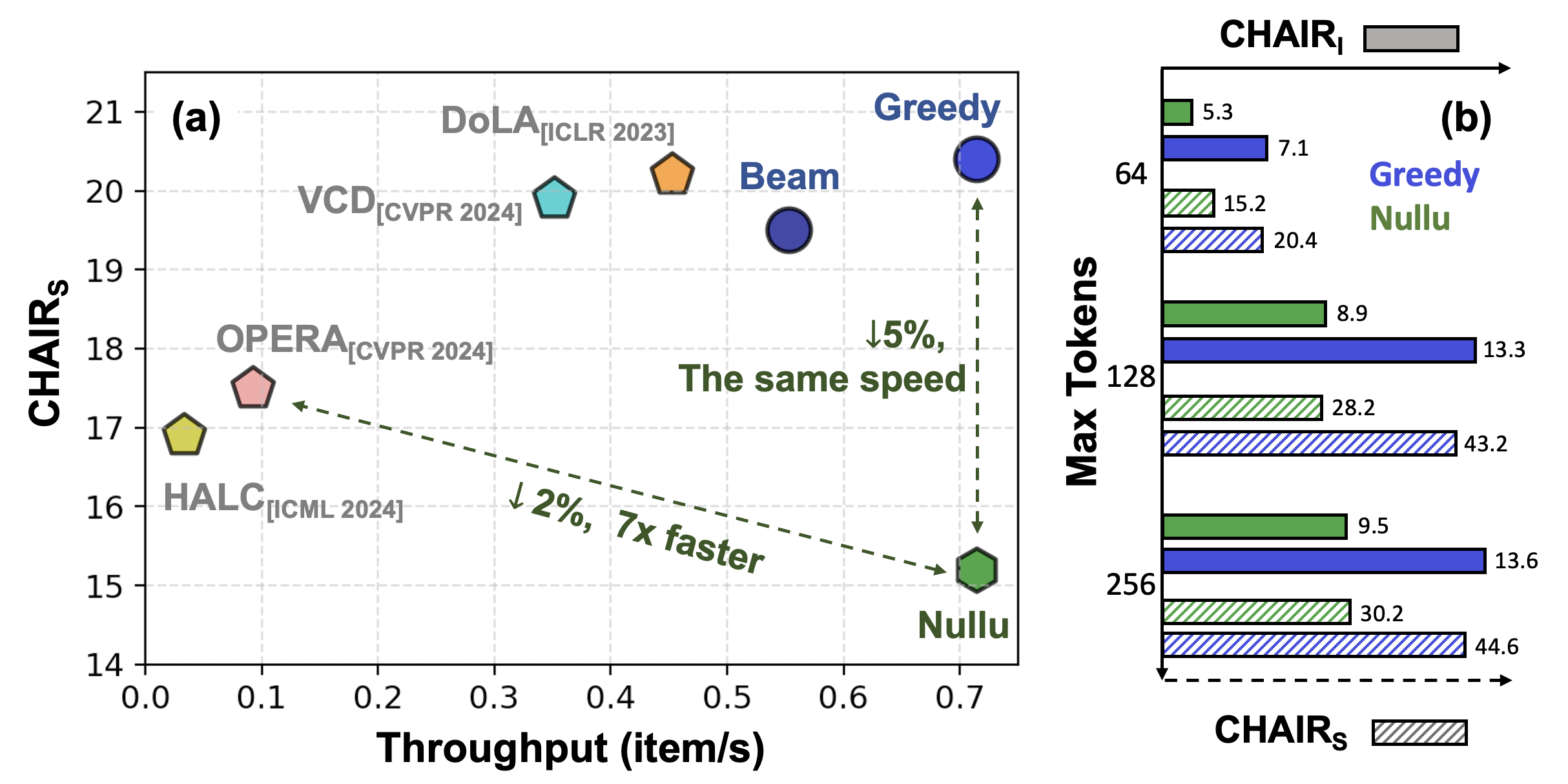
Figure 4: (a) The throughput (tested on NVIDIA RTX 4090) v.s. CHAIR_S. (b) Performance with different max token numbers.

We provide the experimental results in Table 3.4, from which we see that our proposed Nullu consistently outperforms the evaluated methods by a large margin in mitigating OH, demonstrating the effectiveness of Nullu. Moreover, we compared our method to a series of baseline models on LLaVA-1.5 with different numbers of max tokens, and the results are shown in Figure 4 (b). Results show that more output tokens lead to more hallucinations in the responses. While the proposed Nullu still outperforms the baseline model by maintaining a low ratio of hallucination with longer responses and more generated objects.

A unique advantage of Nullu is that it uses the reparameterization technique to load the edited model weights to the original model and, therefore, introduces no extra inference costs. However, most post-hoc OH mitigation methods need to modify the final inference procedure by either debiasing the LLM biases with double-inference [24], or even using multiple adaptive inference procedures [9], and therefore introduce plenty of extra costs during inference. We test the inference speed of different methods, including DoLA [11], VCD [24], and HALC [9] along with the original LLaVA-1.5 with greedy and beam search decoding strategies. The results are shown in Figure 4 (a), which show that Nullu can achieve lower $\text{CHAIR}_{S}$ with faster inference speed. Compared to LLaVA-1.5 with greedy decoding strategy, Nullu can decrease the CHAIR_S by over 5% with the same throughput. Although HALC performs well in mitigating OH, it also introduces many extra inference procedures, which slow the inference speed. Compared to OPERA, Nullu can achieve 7$\times$ faster speed while outperforming OPERA in CHAIR_S.

4.3 Results on POPE

Experimental results on POPE under the random, popular, and adversarial settings are summarized in the Supplementary Materials. Here, we mainly provide the results using OPOPE metrics, shown in Table 4.1. All the numbers are averaged results of the three sampling methods (random, popular, and adversarial, as in the original POPE). The results show that Nullu also performs better than all evaluated methods in terms of accuracy, precision, and F score metrics. The experimental results demonstrate the effectiveness of Nullu in OH mitigation and show its broad applicability on different open-source LVLMs.

4.4 Results on MME

With all models exhibiting comparable performance trajectories, we present the results of LLaVA-1.5-7B as a representative to evaluate the general ability of the edited model. From Figure 5, we see that implementing Nullu leads to a consistent enhancement in perception- and recognition-based tasks. Moreover, it is interesting that using Nullu can significantly enhance the LVLM in text-related tasks, such as OCR and Code Sense Reasoning. This may be attributed to the fact that Nullu achieves the similar optimization attempts with DPO [36], which potentially improves LVLMs’ general capacities by eliminating the possible attempts to generate untruthful responses. See more discussions and numerical results in Supplementary materials.

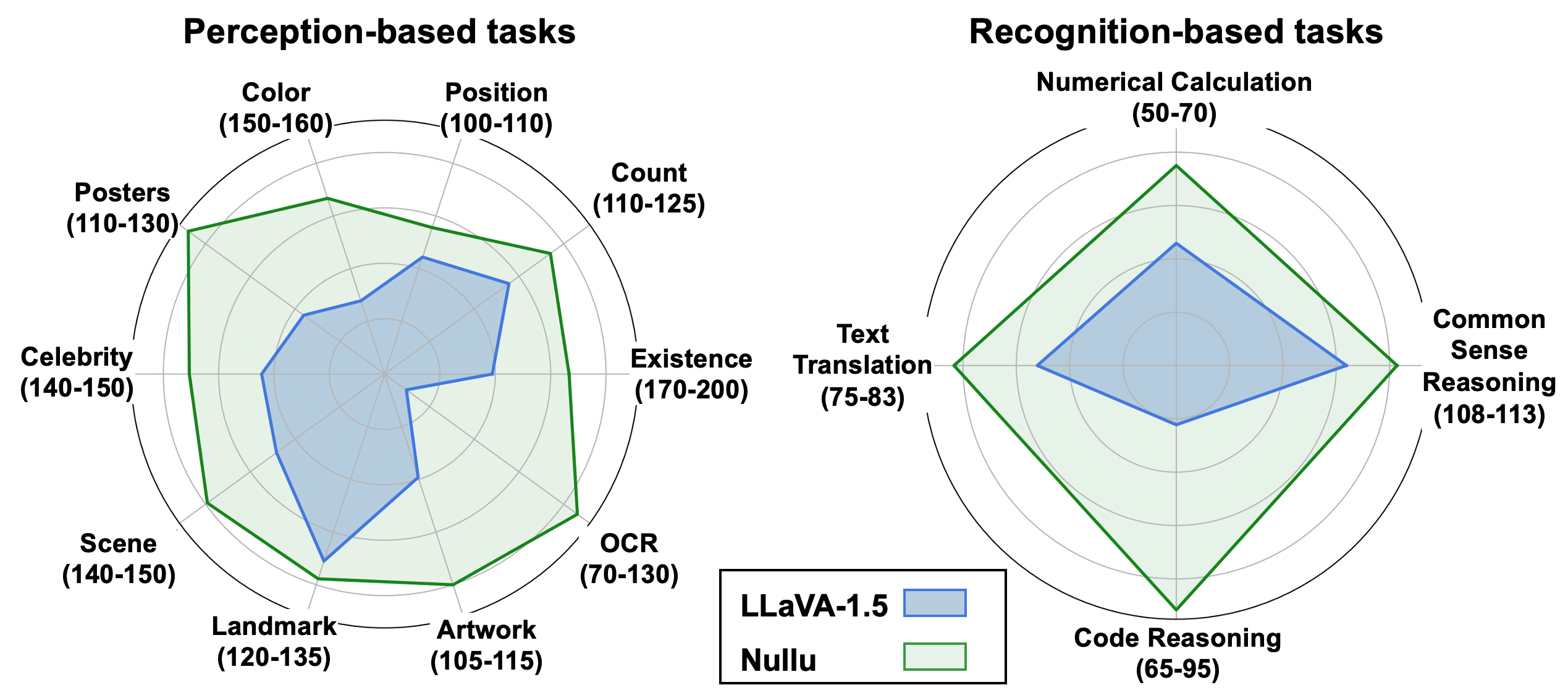
Figure 5: MME full set results on LLaVA-1.5. From the results we see that Nullu leads to consistent improvements of LVLM in both perception tasks and recognition capacities.

4.5 Ablation Studies and Further Analysis

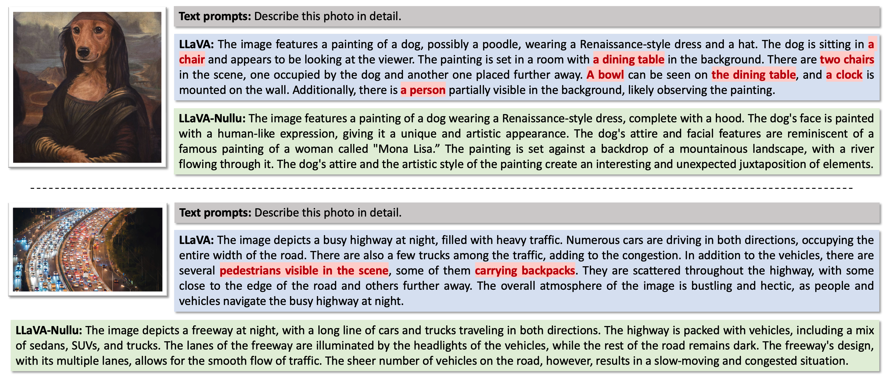
Figure 6: Illustration of hallucination correction by our proposed Nullu with two samples from LLaVA-Bench using LLaVA-1.5-7B. Hallucinated objects from the original model are highlighted in red.

Effects of editing layers $\{\ell\}$ and rank $k$. The proposed Nullu contains two key parameters: the indices of layers needed to be edited $\{\ell\}$ and the selected top-$k$ singular vectors. We test different values of these hyper-parameters with LLaVA-1.5-7B on CHAIR. The results are shown in Table 3. From the results, the editing layers can affect overall performance; therefore, we use $\{\ell\}=\{16,..,32\}$ in all experiments. Moreover, we further found that the performance of Nullu with a larger $k$ to select Top-$k$ singular vectors for building HalluSpace, indicating that the HalluSpace can be possibly with a low-rank structure.

$\{\ell\}$	CS	CI	BLEU	k	CS	CI	BLEU
16-32	15.2	5.30	15.7	2	20.2	7.22	15.3
24-32	16.2	5.58	15.1	4	15.2	5.30	15.7
28-32	18.2	6.27	15.1	8	17.8	5.92	15.2
31-32	16.4	5.59	15.1	16	17.2	6.27	14.8

Table 3: Ablation study of the hyper-parameters in Nullu.

Does HalluSpace represent the hallucination biases? Ideally, if HalluSpace effectively represents these biases, the difference vectors from test samples should have big projected components when mapped onto HalluSpace. To evaluate this, we select 100 test samples from CHAIR where Nullu successfully mitigates OH issues. We compute difference vectors ${\bm{e}}_{i}$ for each sample between the raw and edited LLaVA features. Moreover, we generate 100 random vectors ${\bm{r}}_{i}$ as a comparison baseline. All these vectors are normalized to avoid the effects of norms. Moreover, we use $\sigma_{i}$ to represent the projected components. Figure 7 (a) shows the distribution of vectors on a normalized sphere.

Given ${\bm{V}}_{4}$ (rank-4), each projected component $\sigma_{i}$ resides within $\mathbb{R}^{4}$. We then calculated $\sigma_{i}$ for all selected and random samples, averaging $||\sigma||$ across samples. Figure 7 (b) presents these results, showing that the average $||\sigma||$ of difference vectors across layers is significantly larger (10$\times$) than that of random vectors. Since the selected test samples were successfully edited to avoid OH, this evidence suggests that HalluSpace captures directions in the feature space associated with hallucination and inaccuracies in LVLM responses. More details are available in the Supplementary Materials.

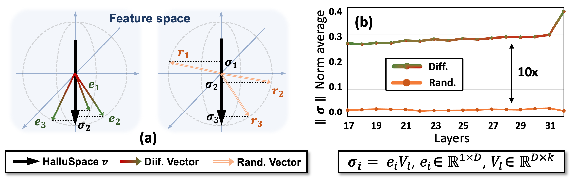
Figure 7: (a) The illustration of experiments. (b) The mean of $||\sigma||$ of 100 test and random vectors at different layers.

Model	Method	Accuracy$\uparrow$	Detailedness$\uparrow$
LLaVA-1.5	Original	$5.89$	$5.02$
	Nullu	6.53	5.59
MiniGPT-4	Original	$4.11$	$4.07$
	Nullu	5.63	4.87
mPLUG-Owl2	Original	$5.96$	$4.52$
	Nullu	6.26	4.72

Table 4: Results of GPT-4V-aided evaluation on LLaVA-Bench following the setting in [24]. Both metrics are on a scale of 10.

GPT-4V Aided Evaluation on LLaVA-Bench. Following previous studies in [24, 49], we leverage LLaVA-Bench [30] to qualitatively evaluate the overall performance using GPT-4V Aided Evaluation. The prompt used for evaluation and an evaluation case is provided in Supplementary Materials. Results in Table 4 show consistent improvements when applying Nullu for each model, demonstrating our method’s effectiveness in both OH mitigation and improving the overall model ability.

Case Study on LLaVA-Bench Figure 6 demonstrates two case studies on LLaVA-1.5-7B given identical prompts and images. The results show that the original LLaVA can yield OH influenced by the statistical bias and language priors inherent during pre-training, as stated in [24]. In the first example, as the model describes the object “chair”, then it hallucinates the frequently co-occurring objects such as “dining table” and “bowl”. A similar issue also happens in the second example, where the model hallucinatedly generates “pedestrians” due to the possible descriptions of the “traffic”. In contrast, using the implementation of Nullu can mitigate these hallucination issues and simultaneously preserve the coherence and informativeness of the output text. More results can be found in our Supplementary Materials.

5 Conclusion and Future Work

In this paper, we proposed a novel method, Nullu, to address OH in modern LVLMs. Nullu extracts HalluSpaces, which are low-rank subspaces of the differences between truthful and hallucinated features, and further edits the LVLMs weights to mitigate OH, resulting in more accurate outputs. Empirical results show that using the edited model weights works to reduce the strong biases in the LLMs, which has been proven as an essential factor for OH. Our theoretical analysis further builds the connection between Nullu and DPO. Experiments demonstrate that Nullu can significantly mitigate OH with no extra inference cost, making it much more efficient than many existing methods and maintaining strong performance in general LVLM benchmarks.

Considering the connection between Nullu and DPO, Nullu can potentially be an alternative but effective way for safety alignment, providing a more efficient and straightforward way to improve LVLMs trustworthiness.

6 The derivation of null space

Here, we give the details about obtaining the null space of the ${\bm{v}}$. We want to proof that: any vector ${\bm{z}}\in\mathbb{R}^{D}$ in the null space of the ${\bm{v}}\in\mathbb{R}^{D}$, $({\bm{I}}-{\bm{v}}{\bm{v}}^{\top})$, is orthogonal to the vector ${\bm{v}}$. Namely, we have ${\bm{v}}^{\top}{\bm{z}}=0$, where ${\bm{v}}$ is the vector with norm 1. ${\bm{I}}$ is the identity matrix with the size of $\mathbb{R}^{D\times D}$. We can write the ${\bm{z}}$ as

$${\bm{z}}=({\bm{I}}-{\bm{v}}{\bm{v}}^{\top}){\bm{m}},\ \ \ \forall{\bm{m}}\in\mathbb{R}^{D}.$$ (8)

Then we have

$${\bm{v}}^{\top}{\bm{z}} ={\bm{v}}^{\top}({\bm{I}}-{\bm{v}}{\bm{v}}^{\top}){\bm{m}}=({\bm{v}}^{\top}-({\bm{v}}^{\top}{\bm{v}}){\bm{v}}^{\top}){\bm{m}},$$ (9)

$$=({\bm{v}}^{\top}-{\bm{v}}^{\top}){\bm{m}}=0,\ \ \forall{\bm{m}}\in\mathbb{R}^{D}.$$ (10)

Therefore, $({\bm{I}}-{\bm{v}}{\bm{v}}^{\top})$ is the null space of ${\bm{v}}$.

7 Decoding information in HalluSpace

layer	Top Tokens
16	dynamic	either	further	above	background	floor	tables	…
17	another	notable	left	later	others	most	tables	…
18	nearby	notable	either	tables	group	optional	others	…
19	notable	middle	either	diverse	background	overall	concentr	…
20	notable	left	nearby	either	background	center	middle	…
21	middle	another	left	bottom	top	left	right	…
22	left	position	middle	another	right	background	top	…
23	notable	left	position	nearby	left	another	bottom	…
24	position	notable	various	various	middle	background	above	…
25	position	towards	left	nearby	right	another	bottom	…
26	in	position	towards	positions	left	nearby	engaged	…
27	in	position	towards	closer	nearby	right	background	…
28	in	the	position	closer	background	nearby	right	…
29	in	position	closer	towards	nearby	background	a	…
30	in	closer	nearby	right	left	another	top	…
31	closer	close	position	bottom	another	left	top	…

Table 5: LLaVA-1.5-7B, top-rank-4, each singular vector of the matrix is interpreted by identifying the top 10 tokens it represents. We use the output embedding vector $e_{j}$ to find top-scoring tokens $j\in\mathcal{V}$ for maximizing $\langle v_{i},e_{j}\rangle$. Tokens have been censored for readability.

As we state in the main paper, to explore the information behind the learned vectors ${\bm{v}}_{i}\in\mathbb{R}^{D}$, a common approach is to decode the embeddings with ${\bm{O}}{\bm{v}}\in\mathbb{R}^{|\mathcal{V}|}$, where ${\bm{O}}=[{\bm{o}}_{1},\ldots,{\bm{o}}_{|\mathcal{V}|}]^{\top}\in\mathbb{R}^{|\mathcal{V}|\times D}$ and $\mathcal{V}$ denotes the vocabulary. We then sort ${\bm{O}}{\bm{v}}$ in ascending order, find the top-$m$ indices, and use the corresponding words to interpret ${\bm{v}}$.

Using Nullu, we can extract the ${\bm{V}}$ at different layers and then decode it via ${\bm{O}}{\bm{v}}$ to explore the internal information behind ${\bm{V}}$. We provide the decoding results in Table. 5. Moreover, we select the words with the most frequency in the output of LVLM with distorted images. For a more straightforward interpretation, we directly selected the words in Table. 5 to see the frequency of words before and after Nullu to see if the LLM biases are mitigated.

8 Theoretical Analysis: How Nullu works?

8.1 Factor component analysis

The analysis is performed for each layer $\ell$, and to avoid the notational burden, we will drop $\ell$ and focus on each layer separately. We use the same notations with these in the main paper. Based on the heuristic in [42], an embedding vector in any transformer layer can be decomposed into interpretable components. We suppose that the generated features ${\bm{f}}_{i}$ can be separated into three different elements:

$${\bm{f}}_{i}\Rightarrow\underbrace{\hat{\bm{f}}_{i}\hat{\bm{B}}}_{\text{truthful contexts}}+\underbrace{\widetilde{\bm{f}}_{i}\widetilde{\bm{B}}}_{\text{hallucinated biases}}+\underbrace{{\bm{u}}_{i}}_{\text{noise}}.$$ (11)

Therefore, give positive and negative samples as input, we have

$${\bm{f}}_{i}^{+}= \underbrace{\hat{\bm{f}}_{i}\hat{\bm{B}}}_{\text{truthful contexts}}+\underbrace{\widetilde{\bm{f}}_{i}\widetilde{\bm{B}}}_{\text{hallucinated biases}} +\underbrace{{\bm{u}}_{i}^{+}}_{\text{noise}}.$$ (12)

$${\bm{f}}_{i}^{-}= \underbrace{\hat{\bm{f}}_{i}\hat{\bm{B}}}_{\text{truthful contexts}} +\underbrace{{\bm{u}}_{i}^{-}}_{\text{noise}},$$ (13)

based on which we have

$${\bm{E}}={\bm{f}}_{i}^{+}-{\bm{f}}_{i}^{-}=\widetilde{\bm{f}}_{i}\widetilde{\bm{B}}+({\bm{u}}_{i}^{+}-{\bm{u}}_{i}^{-}).$$ (14)

The noise can be approximated to 0 on average of the whole data. The top-$k$ singular vectors span exactly the same subspace of $\widetilde{\bm{B}}$, which can be the HalluSpace in our paper. Moreover, SVD is also efficient since SVD gives the best low-rank approximation of ${\bm{E}}$. Thus, our approach can be viewed as an approximate recovery of the latent subspace for hallucination semantics.

8.2 Connections to DPO

In this subsection, we try to establish the conceptual connection between DPO [36] and the proposed Nullu. Our study is mainly based on the theoretical analysis in [42], where a simple logistic model for the output token given the (continuing) prompt is used. In the following parts, we will drop $\ell$ and focus on each layer separately to avoid notational burden.

Although the proposed Nullu is designed for LVLMs, we mainly study its LLM parts, since our weight editing is mainly conducted on this part. Therefore, in this section, we use the term input to denote the extracted features ${\bm{x}}$, containing both the visual features processed by the previous visual encoder, and the text prompts projected into the embedding space. Given ${\bm{x}}$ with hallucinated response $y^{+}$ and truthful response $y^{-}$, where the corresponding embedding features denoted as ${\bm{x}},{\bm{y}}^{+},{\bm{y}}^{-}$ respectively, DPO optimizes the loss

$$\mathcal{L}_{\text{DPO}}(\pi_{\bm{\theta}};\pi_{\text{ref}})= -\mathbb{E}_{(x,y^{+},y^{-})\sim\cal D}[\log\sigma(\beta\log\dfrac{\pi_{\theta}({\bm{y}}^{+}|{\bm{x}})}{\pi_{\text{ref}}({\bm{y}}^{+}|{\bm{x}})}$$

$$-\beta\log\dfrac{\pi_{\theta}({\bm{y}}^{-}|{\bm{x}})}{\pi_{\text{ref}}({\bm{y}}^{-}|{\bm{x}})})],$$ (15)

where, $\pi_{\text{ref}}$ corresponds to the reference (or base) probability model generating output $y$ given $x$, $\pi_{\bm{\theta}}$ is the new probability model (parametrized by ${\bm{\theta}}$), $\sigma$ is the logistic function with $\sigma(z)=(1+\exp(-z))^{-1}$, and $\beta>0$ is a hyperparameter. The gradient of the loss $\mathcal{L}_{\text{DPO}}$ with respect to $\theta$ at initialization $\pi_{\theta}=\pi_{\text{ref}}$ equals

$$\nabla_{\bm{\theta}}\cal L_{\text{DPO}}(\pi_{\bm{\theta}};\pi_{\text{ref}})\mid_{\pi_{\bm{\theta}}=\pi_{\text{ref}}}$$

$$=-\beta\mathbb{E}_{(x,y^{+},y^{-})\sim\cal D}[\nabla_{\bm{\theta}}\log\pi({\bm{y}}^{+}|{\bm{x}})-\nabla_{\bm{\theta}}\log\pi({\bm{y}}^{-}|{\bm{x}})]\mid_{\pi_{\theta}=\pi_{\text{ref}}}.$$ (16)

Let $\cal V$ denote the vocabulary. We start with an input $x$ (including both textual and visual features) and produce $M$ next-token predictions $y_{1},\cdots,y_{M}\in\cal V$ sequentially. Suppose the model sequentially predicts token $y_{m}$ given $x_{m}:=(x,y_{1},\cdots,y_{m-1})$ for each $1\leq m\leq M$, and let ${\bm{x}}_{m}$ denote the encoding of input $x_{m}$. We assume a logistic model generating each continuation $y_{m}$ given $x_{m}$,

$$\pi_{\bm{\theta}}(y_{m}|x_{m})\equiv\pi_{\bm{W}}(y_{m}|x_{m})=Z_{m,{\bm{W}}}^{-1}\exp\left({\bm{o}}_{y_{m}}^{\top}{\bm{W}}{\bm{x}}_{m}\right).$$ (17)

Here, ${\bm{o}}_{y_{m}}$ is the classification vector which we use to get the final word prediction, ${\bm{W}}$ is a weight matrix and $Z_{m,{\bm{W}}}$ is the normalizing constant:

$$Z_{m,{\bm{W}}} =\sum_{y\in\cal V}\exp\left({\bm{o}}_{y}^{\top}{\bm{W}}{\bm{x}}_{m}\right).$$

For the results in Eq. (17), we have assumed for simplicity that the classification is performed with linearly transformed encoding ${\bm{W}}{\bm{x}}_{m}$ instead of the more common non-linear transformations in the transformer architecture. And the output probability is given by the logistic model, based on which we can obtain the joint probability of observing the entire continuation $y=(y_{1},\cdots,y_{M})$ given the starting input $x$ as

$$\pi_{\bm{\theta}}(y|x) \equiv\pi_{\bm{W}}(y|x)=\prod_{m=1}^{M}\pi_{\bm{W}}(y_{m}|x_{m})$$

$$=Z_{\bm{W}}^{-1}\exp\left(\sum_{m=1}^{M}{\bm{o}}_{y_{m}}^{\top}{\bm{W}}{\bm{x}}_{m}\right),$$

where $Z_{\bm{W}}=\prod_{m=1}^{M}Z_{m,{\bm{W}}}$. We denote by $x_{m}^{\pm}$, ${\bm{x}}_{m}^{\pm}$ and ${\bm{o}}_{y_{m}}^{\pm}$ the positive/negative inputs, the corresponding embedding and classification vector for the positive/negative continuation respectively. Plugging this into (8.2), the first step DPO update has gradient

$$\nabla_{\bm{W}}\mathcal{L}_{\text{DPO}}(\pi_{\bm{W}};\pi_{\text{ref}})|_{\pi_{\bm{W}}=\pi_{\text{ref}}}$$

$$=-\beta\mathbb{E}_{(x,y^{+},y^{-})\sim\cal D}\left[\sum_{m=1}^{M}\left({\bm{o}}_{y_{m}}^{+}({\bm{x}}_{m}^{+})^{\top}-{\bm{o}}_{{\bm{y}}_{m}}^{-}({\bm{x}}_{m}^{-})^{\top}\right)\right].$$ (18)

Note that the the normalization factors $Z_{m,{\bm{W}}}$ (and hence $Z_{\bm{W}}$) are omitted when we take the difference of the gradients of the log-probabilities. With $N$ pairs of inputs in $\cal D$, and we consider the case $M=1$, the DPO gradient will be an average over all the pairs:

$$\nabla_{\bm{W}}\mathcal{L}_{\text{DPO}}(\pi_{\bm{W}};\pi_{\text{ref}})|_{\pi_{\bm{W}}=\pi_{\text{ref}}}=-\dfrac{\beta}{N}\sum_{i=1}^{N}({\bm{o}}_{y_{i}}^{+}({\bm{x}}_{i}^{+})^{\top}-{\bm{o}}_{y_{i}}^{-}({\bm{x}}_{i}^{-})^{\top}),$$ (19)

where the extra index $i$ mean $i$-th sample pairs. The Eq.(19) is the formulation (7) in our main paper, which is

$$\nabla_{{\bm{W}}}\mathcal{L}_{\text{DPO}}=-\frac{\beta}{N}\sum_{i=1}^{N}\big{(}{\bm{o}}_{y_{i}^{+}}({\bm{x}}_{i}^{+})^{\top}-{\bm{o}}_{y_{i}^{-}}({\bm{x}}_{i}^{-})^{\top}\big{)}$$

$$= -\frac{\beta}{N}\sum_{i=1}^{N}\big{(}\underbrace{{\bm{o}}_{y_{i}^{+}}({\bm{x}}_{i}^{+}-{\bm{x}}_{i}^{-})^{\top}}_{\text{feature difference}}+\underbrace{({\bm{o}}_{y_{i}^{+}}-{\bm{o}}_{y_{i}^{-}})({\bm{x}}_{i}^{-})^{\top}}_{\text{output difference}}\big{)}.$$ (20)

The gradient contains a feature difference term. Therefore, the gradient update can be interpreted as an attempt to eliminate feature differences to avoid hallucinated responses. For Nullu, it tries to approximate such difference via SVD and also attempts to eliminate it by null space projection, which shows the connection between Nullu and DPO.

9 Implementation Details of LVLMs

This section details the implementation of the evaluated LVLMs and the methods used for OH mitigation. The overall experimental setup is summarized in Table 6. Unlike the standard greedy method, which selects the most probable token at each decoding step, beam search maintains a fixed number of candidate sequences (beams) per step, ranking them based on the accumulated probability scores of the previous tokens $(y_{<t})$. In our experiments, the beam search method uses a num-beams setting of 3, specifying the number of candidate sequences retained at each step. We use the default code for implementation of these two baselines in HuggingFace Transformers Repository[44].

Parameters	Value
Do-sample	False
Num-beams (for beam search)	$3$
Maximum New Tokens (CHAIR)	$64$
Maximum New Tokens (POPE)	$64$
Maximum New Tokens (MME)	$128$
Maximum New Tokens (OPOPE)	$256$
Maximum New Tokens (LLaVA-Bench)	$1024$

Table 6: Hyper-parameters for LVLMs.

The complete hyper-parameters for Nullu across different models in our experiments are as follows. Specifically, there are three major hyper-parameters that can be actively adjusted to optimize Nullu’s effectiveness across different models:

1. Editing Layers $\ell$: For all models, the editing layers range from 16 to 31.

2. The Selected Top-k singular vector: The number of top-k singular vectors selected varies depending on the model. We use the value 4 for LLaVA-1.5 on both CHAIR and POPE. Similarly, we use 8 for MiniGPT-4 on the evaluated two datasets. For mPLUG-Owl2, we use 32 on CHAIR and 16 on POPE.

3. Num-beams: This parameter also differs across models. It is set to 3 for both LLaVA-1.5 and MiniGPT-4, while for mPLUG-Owl2, it is set to 1.

For the comparison of Nullu with SOTAs methods specifically designed for OH mitigation, the evaluation code is built based on the public repository of HALC [9]. Specifically, the hyper-parameters for HALC, DoLa [11], OPERA [18] and VCD [24] are reported in Table 7, Table 9, Table 10 and Table 8, respectively. For each of these baselines, we follow their official implementations and utilize the pre-trained models and configurations provided in their respective repositories, as outlined in their papers, to reproduce the reported results.

Parameters	Value
Amplification Factor $\alpha$	$0.05$
JSD Buffer Size $m$	$6$
Beam Size	$1$
FOV Sampling	Exponential Expansion
Number of Sampled FOVs $n$	$4$
Exponential Growth Factor $\lambda$	0.6
Adaptive Plausibility Threshold	$0.1$

Table 7: HALC Hyperparameter Settings

Parameters	Value
Amplification Factor $\alpha$	$1$
Adaptive Plausibility Threshold $\beta$	$0.1$
Diffusion Noise Step	$500$

Table 8: VCD Hyperparameter Settings

Parameters	Value
Repetition Penalty $\theta$	$1.2$
Adaptive Plausibility Threshold $\beta$	$0.1$
Pre-mature Layers	$[0,2\cdots,32]$

Table 9: DoLa Hyperparameter Settings

Parameters	Value
Self-attention Weights Scale Factor $\theta$	$50$
Attending Retrospection Threshold	$15$
Beam Size	$3$
Penalty Weights	$1$

Table 10: OPERA Hyperparameter Settings

10 POPE Settings and Additional Results

Polling-based Object Probing Evaluation (POPE) [27], presents a streamlined approach to assess object hallucination. POPE interacts directly with the examined LVLM, which distinguishes it from CHAIR. Within this benchmark, LVLMs are queried to answer if a specific object exists in the given image. The ratio between queries probing existent objects and non-existent objects is balanced (i.e.,$50$% vs. $50$%). It encompasses three sampling settings: random, popular, and adversarial, each distinct in constructing negative samples. In the random setting, objects absent from the image are chosen randomly. The popular setting selects missing objects from a high-frequency pool, while in the adversarial setting, co-occurring objects not present in the image are prioritized. We use the POPE benchmark aggregates data from MSCOCO [28]. It involves $500$ images from each dataset under each sampling setting and formulates $6$ questions per image. The evaluation pivots on four key metrics: Accuracy, Precision, Recall, and the F1 score.

10.1 POPE Results

Setting	Model	Method	Accuracy	Precision	Recall	$\text{F}_{\text{1}}$ Score
Random	MiniGPT4	Greedy	64.33	58.66	97.13	73.14
		Beam Search	62.10	57.15	96.67	71.84
		DoLa	64.27	58.82	95.10	72.68
		VCD	57.90	55.69	77.27	64.73
		HALC	64.87	59.04	97.13	73.44
		Nullu	77.23	76.54	78.53	77.53
Popular	MiniGPT4	Greedy	56.63	53.66	97.13	69.13
		Beam Search	56.47	53.58	96.67	68.95
		DoLa	56.58	53.72	95.10	68.65
		VCD	55.30	53.59	79.20	63.92
		HALC	57.00	53.88	97.13	69.31
		Nullu	70.13	67.24	78.53	72.45
Adversarial	MiniGPT4	Greedy	55.17	52.81	97.13	68.42
		Beam Search	55.50	53.02	96.67	68.48
		DoLa	55.85	53.28	95.10	68.29
		VCD	52.90	51.99	75.60	61.61
		HALC	55.53	53.02	97.13	68.60
		Nullu	66.70	63.50	78.53	70.22

Table 11: POPE results with random, popular and adversarial samplings compared to existing OH mitigation methods.

We conduct the comparison between the raw LVLMs and the one implemented with Nullu on POPE and provide the results in Table 12.

Setting	Model	Method	Accuracy	Precision	Recall	$\textbf{F}_{\textbf{1}}$ Score
random	LLaVA-1.5	Original	88.98	88.65	89.43	89.03
		Nullu	89.45	91.41	87.10	89.20
	MiniGPT4	Original	64.33	58.66	97.13	73.14
		Nullu	77.23	76.54	78.53	77.53
	mPLUG-Owl2	Original	81.83	77.80	89.07	83.06
		Nullu	83.33	79.10	90.60	84.46
popular	LLaVA-1.5	Original	84.58	81.61	89.43	85.32
		Nullu	85.37	84.25	87.10	85.63
	MiniGPT4	Original	56.63	53.66	97.13	69.13
		Nullu	70.13	67.24	78.53	72.45
	mPLUG-Owl2	Original	75.77	70.35	89.07	78.61
		Nullu	77.47	71.75	90.60	80.08
adversarial	LLaVA-1.5	Original	77.97	72.79	89.43	80.24
		Nullu	79.40	75.51	87.10	80.88
	MiniGPT4	Original	55.17	52.81	97.13	68.42
		Nullu	66.70	63.50	78.53	70.22
	mPLUG-Owl2	Original	72.77	67.17	89.07	76.58
		Nullu	74.03	68.05	90.60	77.72

Table 12: Results on POPE. Original denotes direct sampling for LVLMs, whereas Nullu refers to edit the model with the proposed method.

We also tested different OH methods on MiniGPT-4 and provided the results in Table 11. The results show that Nullu outperforms all other methods by a significant margin regarding the accuracy and F1 score across all three types of POPE VQA tasks (random, popular, adversarial). Our experiments show that the MiniGPT-4 tends to provide the answer with “yes”, which leads to a high recall ratio for most tested OH methods. However, the Precision of these methods is generally lower than 60%, resulting in a lower F1 score. However, Nullu significantly improves the Precision of the Mini-GPT, resulting in a noticeable improvement in the F1 score. Moreover, we also see that VCD also has a lower recall, indicating that the LLM bias of Mini-GPT makes the model tend to provide the answer with “yes” when responding.

Setting	Model	Method	Accuracy	Precision	Recall	F Score
Random	LLaVA-1.5	Greedy	81.52	98.41	64.07	96.42
		Beam Search	81.67	98.67	64.20	96.67
		DoLa	81.38	98.11	64.00	96.14
		OPERA	81.62	98.57	64.17	96.58
		VCD	80.57	98.41	62.13	96.25
		HALC	79.58	98.21	60.27	95.89
		Nullu	81.18	98.05	63.63	96.05
	MiniGPT-4	Greedy	72.42	98.49	45.53	94.25
		Beam Search	72.65	98.70	45.90	94.51
		DoLa	72.45	98.58	45.57	94.34
		OPERA	72.57	98.77	45.70	94.52
		VCD	72.35	98.19	45.53	93.97
		HALC	72.08	98.62	44.80	94.25
		Nullu	72.68	99.06	45.80	94.82
	mPLUG-Owl2	Greedy	79.45	97.74	60.30	95.46
		Beam Search	79.45	97.52	60.43	95.27
		DoLa	78.33	97.60	58.10	95.09
		OPERA	78.31	97.73	57.96	95.21
		VCD	78.19	98.23	57.42	95.61
		HALC	77.83	97.72	57.00	95.10
		Nullu	80.30	98.40	61.60	96.19
Popular	LLaVA-1.5	Greedy	78.93	91.17	64.07	89.71
		Beam Search	79.30	91.98	64.20	90.47
		DoLa	78.72	90.69	64.00	89.26
		OPERA	79.22	91.80	64.17	90.30
		VCD	77.57	89.87	62.13	88.35
		HALC	77.47	91.87	60.27	90.05
		Nullu	79.80	94.06	63.63	92.36
	MiniGPT-4	Greedy	70.80	92.01	45.53	88.53
		Beam Search	71.32	93.35	45.90	89.77
		DoLa	70.90	92.33	45.57	88.82
		OPERA	71.10	92.82	45.70	89.27
		VCD	70.33	90.30	45.53	86.98
		HALC	70.92	93.80	44.80	90.00
		Nullu	71.97	96.08	45.80	92.19
	mPLUG-Owl2	Greedy	76.00	87.90	60.30	86.38
		Beam Search	75.90	87.50	60.43	86.02
		DoLa	75.20	88.36	58.10	86.60
		OPERA	75.02	88.06	57.96	86.33
		VCD	74.86	88.16	57.42	86.37
		HALC	75.77	91.34	57.00	89.26
		Nullu	78.20	92.22	61.60	90.49
Adversarial	LLaVA-1.5	Greedy	76.97	86.36	64.07	85.22
		Beam Search	77.27	86.92	64.20	85.75
		DoLa	76.85	86.18	64.00	85.05
		OPERA	77.03	86.40	64.17	85.26
		VCD	75.88	85.71	62.13	84.48
		HALC	76.57	89.44	60.27	87.80
		Nullu	77.58	88.27	63.63	86.98
	MiniGPT-4	Greedy	70.43	90.65	45.53	87.32
		Beam Search	70.98	92.06	45.90	88.63
		DoLa	70.50	90.85	45.57	87.50
		OPERA	70.78	91.63	45.70	88.21
		VCD	69.82	88.43	45.53	85.32
		HALC	70.52	92.22	44.80	88.60
		Nullu	71.10	92.73	45.80	89.21
	mPLUG-Owl2	Greedy	74.23	83.58	60.30	82.36
		Beam Search	73.78	82.51	60.43	81.37
		DoLa	73.52	83.98	58.10	82.55
		OPERA	73.17	83.45	57.96	82.06
		VCD	72.85	83.01	57.42	81.61
		HALC	74.02	86.41	57.00	84.72
		Nullu	76.90	88.76	61.60	87.28

Table 13: Detailed OPOPE results with random, popular and adversarial samplings.

10.2 OPOPE results

While this interaction is not problematic for evaluating decoding-based baselines, it limits the applicability of POPE to post-hoc OH mitigation methods. This direct interaction also creates greater instability when the examined LVLM is based on smaller language backbones, such as LLaMA-7B, which has less robust chat capabilities. To address these issues, offline POPE (OPOPE) was introduced in HALC [9], where a comparison is made between this approach and other effective decoding methods.

Since OPOPE evaluates directly based on the caption generated for each image, it follows the caption generation procedure from CHAIR but differs in the subsequent metric calculation. When computing the OPOPE scores, we follow the processing procedure of CHAIR while adopting POPE’s metric calculation methodology.

For every sampled 500 images in the validation split of MSCOCO. The captions generated by the models are tokenized separately and then each word is singularized. Subsequently, the words are mapped to MSCOCO objects using the synonym and double-word lists provided in [37].

Next, three hallucination test object lists are constructed following the sampling strategies proposed in the POPE method. We refer detailed explanations of the different options to its original paper[27]. Each list contains six objects, with a 1:1 ratio of ground-truth to nonexistent objects to ensure label balance. These lists are originally used to generate polling questions based on the template “Is there a/an {} in the image?” in [27].

After obtaining the objects set from the generated captions and the three test objects list, we assess whether the captions include the ground-truth or nonexistent objects. The comparison results are used to compute scores as the score of the corresponding sampling strategy setting.

The primary metric in OPOPE is modified to enable more reliable comparisons. Since offline evaluations are less likely to include the exact hallucinated objects in descriptions, false negatives (FNs) and the resulting recall become less reliable. To address this, and in line with HALC, we adopt F-beta as the main metric for OPOPE instead of F-1, reducing the emphasis on FNs. Specifically, the F-beta score is defined as: $F_{\beta}=(1+\beta^{2})\cdot(\text{precision}\cdot\text{recall})/(\beta^{2}\cdot\text{precision}+\text{recall})$, where $\beta=0.2$ is used throughout our experiments following [9].

The detailed and comprehensive evaluation results under each sampling strategy incorporating OPOPE are presented in Table 13. From the results, we see that our method achieve 7 best results (denoted by bold) in 9 comparisons, which again demonstrates the effectiveness of our method.

11 MME Numerical Results

Model	Method	Existence	Count	Position	Color	Posters		Perception Total
LLaVA-1.5	Original	$181.67_{\pm 2.36}$	$118.33_{\pm 12.47}$	$104.44_{\pm 10.39}$	$152.78_{\pm 5.67}$	$117.23_{\pm 4.79}$	Original	$1246.36_{\pm 5.79}$
	Nullu	$\textbf{190.00}_{\pm 4.08}$	$\textbf{121.11}_{\pm 7.74}$	$\textbf{105.56}_{\pm 8.20}$	$\textbf{156.67}_{\pm 9.81}$	$\textbf{127.55}_{\pm 4.20}$
Model	Method	Celebrity	Scene	Landmark	Artwork	OCR	Nullu	$\textbf{1330.71}_{\pm 19.77}$
LLaVA-1.5	Original	$111.67_{\pm 3.90}$	$144.83_{\pm 1.50}$	$130.65_{\pm 5.26}$	$108.92_{\pm 2.99}$	$75.83_{\pm 5.89}$
	Nullu	$\textbf{115.59}_{\pm 6.60}$	$\textbf{147.92}_{\pm 1.36}$	$\textbf{131.66}_{\pm 1.09}$	$\textbf{113.00}_{\pm 2.07}$	$\textbf{121.67}_{\pm 8.25}$

Table 14: Results on all MME perception-related tasks.

Model	Method	Common Sense Reasoning	Numerical Calculation	Text Translation	Code Reasoning	Recognition Total
LLaVA-1.5	Original	$111.19_{\pm 4.68}$	$59.17_{\pm 7.73}$	$79.17_{\pm 8.25}$	$71.67_{\pm 11.24}$	$321.19_{\pm 2.15}$
	Nullu	$\textbf{112.14}_{\pm 3.55}$	$\textbf{65.00}_{\pm 16.20}$	$\textbf{81.67}_{\pm 7.73}$	$\textbf{92.50}_{\pm 15.94}$	$\textbf{351.31}_{\pm 2.61}$

Table 15: Results on all MME recognition-related tasks.

In Table 14, we present the performance of the edited LLaVA-1.5 baselines on the perception-related tasks of the MME benchmark.

The baselines demonstrate consistent performance patterns, with Nullu uniformly improving the perceptual competencies of the LVLM model. Specifically, the edited model shows improvement for tasks typically used to estimate hallucination capability [9], including color, existence, count, and position. Furthermore, likely due to Nullu’s effect in alleviating language priors, the model exhibits enhancements across all tasks, particularly in OCR, achieving an additional 84.35-point improvement in the total score. Furthermore, Table 15 showcases the performances on recognition-related tasks within the MME benchmark. The results suggest that implementing Nullu while mitigating hallucination issues and enhancing perceptual capabilities does not compromise the inherent reasoning abilities of LVLM. This is evident from the consistent overall recognition scores, which indicate that the model’s fidelity remains unaffected by the intervention. Nullu significantly surpasses the original model, demonstrating a comprehensive performance improvement in reducing OH while maintaining generation quality.

12 Analysis about HalluSpace

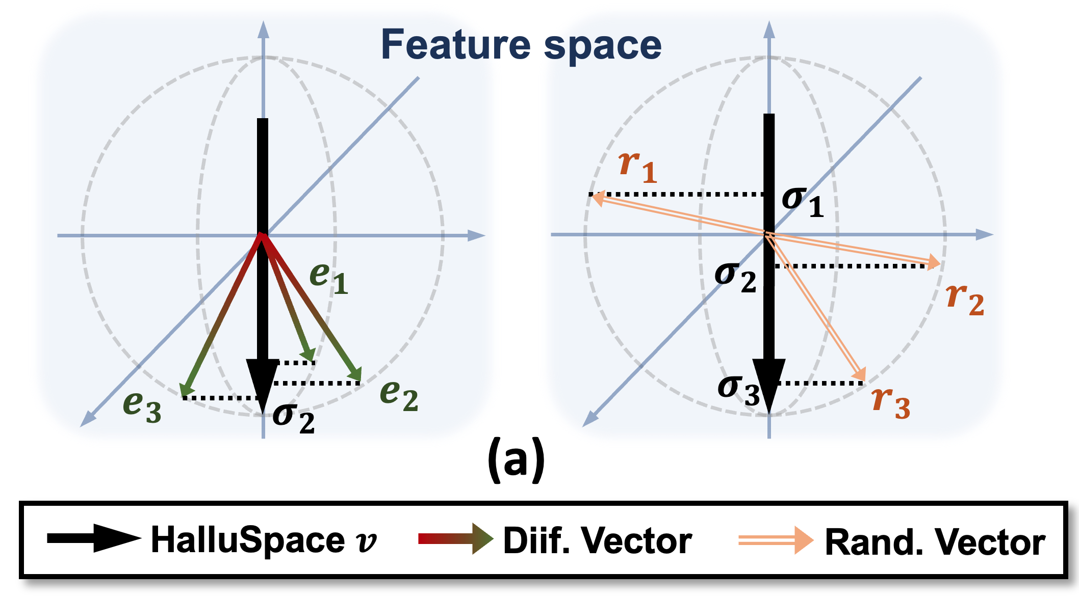
Figure 8: The illustration of difference vectors and random vectors in the feature space.

This section provides a more comprehensive study about the question Does HalluSpace represent the hallucination biases?. In other words, can the HalluSpace learned from the prepared hallucinated pairs adequately represent the true OH during the test? Ideally, if HalluSpace effectively represents these biases, the difference vectors from test samples with few OH issues after editing should have larger projected components when mapped onto HalluSpace than these random ones. Indeed, if the HalluSpace represents the OH problematic direction, the aforementioned difference vectors from test samples should gather together around this direction. This is further illustrated in Figure. 8.

To evaluate this, we select 100 test samples from CHAIR where Nullu successfully mitigates OH issues. We compute difference vectors ${\bm{e}}_{i}$ for each sample between the raw and edited LLaVA features. Moreover, we generate 100 random vectors ${\bm{r}}_{i}$ as a comparison baseline. All these vectors are normalized to avoid the effects of norms. Moreover, we use $\sigma_{i}$ to represent the projected components. Figure. 8 shows the distribution of vectors on a normalized sphere.

Given ${\bm{V}}_{4}$ (rank-4), each projected component $\sigma_{i}$ resides within $\mathbb{R}^{4}$. We then calculated $\sigma_{i}={\bm{e}}_{i}{\bm{V}}_{4}$ for all selected samples and random vectors ($\sigma_{i}={\bm{r}}_{i}{\bm{V}}_{4}$), averaging $||\sigma||$ across samples. The results is provided in Table.16. The table shows that the average $||\sigma||$ of difference vectors across layers is significantly larger (10$\times$) than that of random vectors. Since the selected test samples were successfully edited to avoid OH, this evidence suggests that HalluSpace captures directions in the feature space associated with hallucination and inaccuracies in LVLM responses.

Layers	17	18	19	20	21	22	23	24	25	26	27	28	29	30	31	32
Diff.	0.269	0.266	0.270	0.270	0.279	0.278	0.284	0.279	0.287	0.283	0.288	0.292	0.291	0.293	0.300	0.386
Rand	0.023	0.025	0.027	0.026	0.026	0.021	0.022	0.022	0.023	0.025	0.027	0.026	0.025	0.029	0.030	0.021

Table 16: Norm average of difference vectors and random vectors at different layers in the LVLM.

13 LLaVA-Bench

13.1 Prompt for GPT-4V Aided Evaluation

As we leverage LLaVA-Bench [30] to qualitatively evaluate the overall performance using GPT-4V Aided Evaluation, in this section, we main describe the prompt used for evaluation. The assessments using GPT-4V are based on the accuracy and level of detail in the responses generated by LVLMs, following the approach described in [24]. The specific prompt structure is detailed in Table 17. During the evaluation, we collect the responses from two different LVLMS and then use the responses to replace the “{Response}” in the prompt, which is then sent to GPT-4V to conduct the evaluation. Next, we can collect the GPT4-V Output to evaluate the accuracy and detailedness of the responses from two different LVLMs. We further provide an evaluation example in Table 18 to further illustrate this process.

Table 17: The configuration to build an image-description evaluator with GPT-4V

Table 18: Evaluation example for the image-description evaluator with GPT-4V.

13.2 More case studies

Additional case studies on the LLaVA-bench are presented in Figure 10 and Figure 11 to illustrate the effectiveness of our approach. Note that the case in Figure 11 provides an example that the proposed Nullu can correctly generate an HTML script that meets the need in the text prompts, which also corresponds to the experimental results on MME, where the edited model is shown that can achieve better performance in Code Reasoning tasks, further demonstrating the effectiveness of our method. The generated HTML website is shown in Figure 9.

Figure 9: The generated website of Nullu.

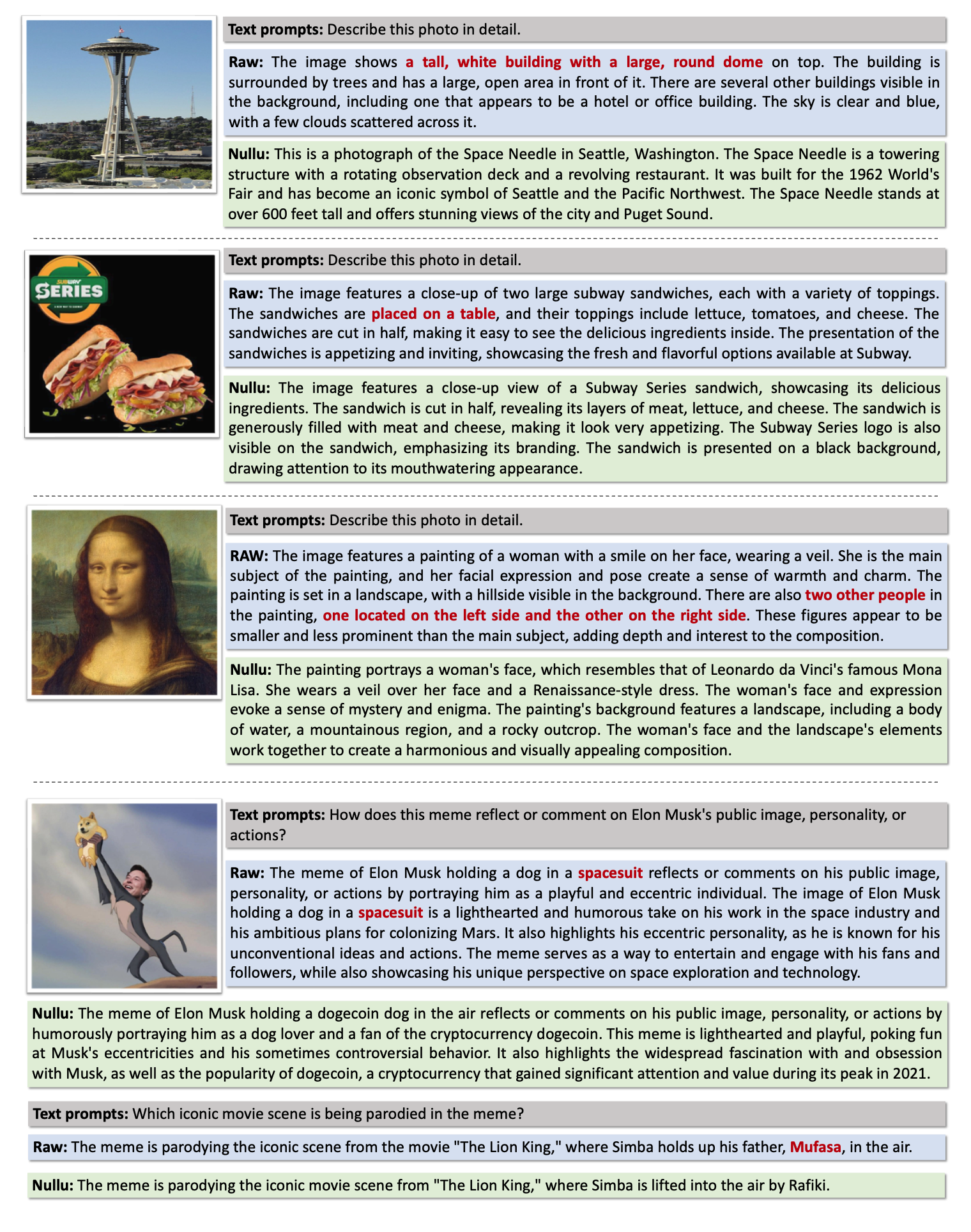
Figure 10: More examples of Nullu on LLaVA-Bench.

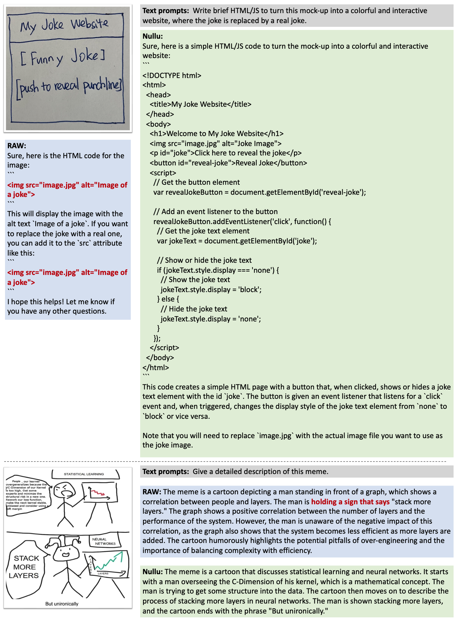
Figure 11: More examples of Nullu on LLaVA-Bench.

References

- Achiam et al. [2023] Josh Achiam, Steven Adler, Sandhini Agarwal, Lama Ahmad, Ilge Akkaya, Florencia Leoni Aleman, Diogo Almeida, Janko Altenschmidt, Sam Altman, Shyamal Anadkat, et al. Gpt-4 technical report. arXiv preprint arXiv:2303.08774, 2023.
- Bai et al. [2023a] Jinze Bai, Shuai Bai, Yunfei Chu, Zeyu Cui, Kai Dang, Xiaodong Deng, Yang Fan, Wenbin Ge, Yu Han, Fei Huang, et al. Qwen technical report. arXiv preprint arXiv:2309.16609, 2023a.
- Bai et al. [2023b] Jinze Bai, Shuai Bai, Shusheng Yang, Shijie Wang, Sinan Tan, Peng Wang, Junyang Lin, Chang Zhou, and Jingren Zhou. Qwen-vl: A frontier large vision-language model with versatile abilities. arXiv preprint arXiv:2308.12966, 2023b.
- Bai et al. [2024] Zechen Bai, Pichao Wang, Tianjun Xiao, Tong He, Zongbo Han, Zheng Zhang, and Mike Zheng Shou. Hallucination of multimodal large language models: A survey. arXiv preprint arXiv:2404.18930, 2024.
- Biten et al. [2022] Ali Furkan Biten, Lluís Gómez, and Dimosthenis Karatzas. Let there be a clock on the beach: Reducing object hallucination in image captioning. In Proceedings of the IEEE/CVF Winter Conference on Applications of Computer Vision, pages 1381–1390, 2022.
- Chen et al. [2023] Keqin Chen, Zhao Zhang, Weili Zeng, Richong Zhang, Feng Zhu, and Rui Zhao. Shikra: Unleashing multimodal llm’s referential dialogue magic. arXiv preprint arXiv:2306.15195, 2023.
- Chen et al. [2024a] Yangyi Chen, Karan Sikka, Michael Cogswell, Heng Ji, and Ajay Divakaran. Dress: Instructing large vision-language models to align and interact with humans via natural language feedback. In IEEE Conf. Comput. Vis. Pattern Recog., pages 14239–14250, 2024a.
- Chen et al. [2024b] Zhe Chen, Jiannan Wu, Wenhai Wang, Weijie Su, Guo Chen, Sen Xing, Muyan Zhong, Qinglong Zhang, Xizhou Zhu, Lewei Lu, et al. Internvl: Scaling up vision foundation models and aligning for generic visual-linguistic tasks. In IEEE Conf. Comput. Vis. Pattern Recog., pages 24185–24198, 2024b.
- Chen et al. [2024c] Zhaorun Chen, Zhuokai Zhao, Hongyin Luo, Huaxiu Yao, Bo Li, and Jiawei Zhou. Halc: Object hallucination reduction via adaptive focal-contrast decoding. In Int. Conf. Machine Learn., 2024c.
- Chiang et al. [2023] Wei-Lin Chiang, Zhuohan Li, Zi Lin, Ying Sheng, Zhanghao Wu, Hao Zhang, Lianmin Zheng, Siyuan Zhuang, Yonghao Zhuang, Joseph E. Gonzalez, Ion Stoica, and Eric P. Xing. Vicuna: An open-source chatbot impressing gpt-4 with 90%* chatgpt quality, 2023.
- Chuang et al. [2023] Yung-Sung Chuang, Yujia Xie, Hongyin Luo, Yoon Kim, James R Glass, and Pengcheng He. Dola: Decoding by contrasting layers improves factuality in large language models. In Int. Conf. Learn. Represent., 2023.
- Devlin et al. [2018] Jacob Devlin, Ming-Wei Chang, Kenton Lee, and Kristina Toutanova. Bert: Pre-training of deep bidirectional transformers for language understanding. arXiv preprint arXiv:1810.04805, 2018.
- Favero et al. [2024] Alessandro Favero, Luca Zancato, Matthew Trager, Siddharth Choudhary, Pramuditha Perera, Alessandro Achille, Ashwin Swaminathan, and Stefano Soatto. Multi-modal hallucination control by visual information grounding. In IEEE Conf. Comput. Vis. Pattern Recog., pages 14303–14312, 2024.
- Freitag and Al-Onaizan [2017] Markus Freitag and Yaser Al-Onaizan. Beam search strategies for neural machine translation. arXiv preprint arXiv:1702.01806, 2017.
- Fu et al. [2023] Chaoyou Fu, Peixian Chen, Yunhang Shen, Yulei Qin, Mengdan Zhang, Xu Lin, Zhenyu Qiu, Wei Lin, Jinrui Yang, Xiawu Zheng, et al. Mme: A comprehensive evaluation benchmark for multimodal large language models. arXiv preprint arXiv:2306.13394, 2023.
- Geva et al. [2021] Mor Geva, Roei Schuster, Jonathan Berant, and Omer Levy. Transformer feed-forward layers are key-value memories. In Adv. Neural Inform. Process. Syst., pages 5484–5495, 2021.
- Gunjal et al. [2024] Anisha Gunjal, Jihan Yin, and Erhan Bas. Detecting and preventing hallucinations in large vision language models. In AAAI, pages 18135–18143, 2024.
- Huang et al. [2024a] Qidong Huang, Xiaoyi Dong, Pan Zhang, Bin Wang, Conghui He, Jiaqi Wang, Dahua Lin, Weiming Zhang, and Nenghai Yu. Opera: Alleviating hallucination in multi-modal large language models via over-trust penalty and retrospection-allocation. In IEEE Conf. Comput. Vis. Pattern Recog., pages 13418–13427, 2024a.
- Huang et al. [2024b] Wen Huang, Hongbin Liu, Minxin Guo, and Neil Zhenqiang Gong. Visual hallucinations of multi-modal large language models. arXiv preprint arXiv:2402.14683, 2024b.
- Jiang et al. [2024] Chaoya Jiang, Haiyang Xu, Mengfan Dong, Jiaxing Chen, Wei Ye, Ming Yan, Qinghao Ye, Ji Zhang, Fei Huang, and Shikun Zhang. Hallucination augmented contrastive learning for multimodal large language model. In IEEE Conf. Comput. Vis. Pattern Recog., pages 27036–27046, 2024.
- Jing and Du [2024] Liqiang Jing and Xinya Du. Fgaif: Aligning large vision-language models with fine-grained ai feedback. arXiv preprint arXiv:2404.05046, 2024.
- Kim et al. [2023] Jae Myung Kim, A Koepke, Cordelia Schmid, and Zeynep Akata. Exposing and mitigating spurious correlations for cross-modal retrieval. In IEEE Conf. Comput. Vis. Pattern Recog., pages 2584–2594, 2023.
- Kim et al. [2024] Moo Jin Kim, Karl Pertsch, Siddharth Karamcheti, Ted Xiao, Ashwin Balakrishna, Suraj Nair, Rafael Rafailov, Ethan Foster, Grace Lam, Pannag Sanketi, et al. Openvla: An open-source vision-language-action model. arXiv preprint arXiv:2406.09246, 2024.
- Leng et al. [2024] Sicong Leng, Hang Zhang, Guanzheng Chen, Xin Li, Shijian Lu, Chunyan Miao, and Lidong Bing. Mitigating object hallucinations in large vision-language models through visual contrastive decoding. In IEEE Conf. Comput. Vis. Pattern Recog., pages 13872–13882, 2024.
- Li et al. [2022] Junnan Li, Dongxu Li, Caiming Xiong, and Steven Hoi. Blip: Bootstrapping language-image pre-training for unified vision-language understanding and generation. In Int. Conf. Machine Learn., pages 12888–12900, 2022.
- Li et al. [2023a] Junnan Li, Dongxu Li, Silvio Savarese, and Steven Hoi. Blip-2: Bootstrapping language-image pre-training with frozen image encoders and large language models. In Int. Conf. Machine Learn., pages 19730–19742, 2023a.
- Li et al. [2023b] Yifan Li, Yifan Du, Kun Zhou, Jinpeng Wang, Wayne Xin Zhao, and Ji-Rong Wen. Evaluating object hallucination in large vision-language models. In Proceedings of the 2023 Conference on Empirical Methods in Natural Language Processing, pages 292–305, 2023b.
- Lin et al. [2014] Tsung-Yi Lin, Michael Maire, Serge Belongie, James Hays, Pietro Perona, Deva Ramanan, Piotr Dollár, and C Lawrence Zitnick. Microsoft coco: Common objects in context. In Computer Vision–ECCV 2014: 13th European Conference, Zurich, Switzerland, September 6-12, 2014, Proceedings, Part V 13, pages 740–755. Springer, 2014.
- Liu et al. [2023a] Fuxiao Liu, Kevin Lin, Linjie Li, Jianfeng Wang, Yaser Yacoob, and Lijuan Wang. Mitigating hallucination in large multi-modal models via robust instruction tuning. arXiv preprint arXiv:2306.14565, 2023a.
- Liu et al. [2023b] Haotian Liu, Chunyuan Li, Yuheng Li, and Yong Jae Lee. Improved baselines with visual instruction tuning. arXiv preprint arXiv:2310.03744, 2023b.
- Liu et al. [2024a] Haotian Liu, Chunyuan Li, Qingyang Wu, and Yong Jae Lee. Visual instruction tuning. Adv. Neural Inform. Process. Syst., 36, 2024a.
- Liu et al. [2024b] Shi Liu, Kecheng Zheng, and Wei Chen. Paying more attention to image: A training-free method for alleviating hallucination in lvlms. In Eur. Conf. Comput. Vis., 2024b.
- Liu et al. [2019] Yinhan Liu, Myle Ott, Naman Goyal, Jingfei Du, Mandar Joshi, Danqi Chen, Omer Levy, Mike Lewis, Luke Zettlemoyer, and Veselin Stoyanov. Roberta: A robustly optimized bert pretraining approach. arXiv preprint arXiv:1907.11692, 2019.
- Lu et al. [2024] Yuhang Lu, Yichen Yao, Jiadong Tu, Jiangnan Shao, Yuexin Ma, and Xinge Zhu. Can lvlms obtain a driver’s license? a benchmark towards reliable agi for autonomous driving. arXiv preprint arXiv:2409.02914, 2024.
- Meta [2024] AI Meta. Introducing meta llama 3: The most capable openly available llm to date. Meta AI Blog (accessed 2024–04–20)., 2024.
- Rafailov et al. [2024] Rafael Rafailov, Archit Sharma, Eric Mitchell, Christopher D Manning, Stefano Ermon, and Chelsea Finn. Direct preference optimization: Your language model is secretly a reward model. Adv. Neural Inform. Process. Syst., 36, 2024.
- Rohrbach et al. [2018] Anna Rohrbach, Lisa Anne Hendricks, Kaylee Burns, Trevor Darrell, and Kate Saenko. Object hallucination in image captioning. arXiv preprint arXiv:1809.02156, 2018.
- Sun et al. [2023] Zhiqing Sun, Sheng Shen, Shengcao Cao, Haotian Liu, Chunyuan Li, Yikang Shen, Chuang Gan, Liang-Yan Gui, Yu-Xiong Wang, Yiming Yang, et al. Aligning large multimodal models with factually augmented rlhf. arXiv preprint arXiv:2309.14525, 2023.
- Team et al. [2023] Gemini Team, Rohan Anil, Sebastian Borgeaud, Yonghui Wu, Jean-Baptiste Alayrac, Jiahui Yu, Radu Soricut, Johan Schalkwyk, Andrew M Dai, Anja Hauth, et al. Gemini: a family of highly capable multimodal models. arXiv preprint arXiv:2312.11805, 2023.
- Touvron et al. [2023a] Hugo Touvron, Thibaut Lavril, Gautier Izacard, Xavier Martinet, Marie-Anne Lachaux, Timothée Lacroix, Baptiste Rozière, Naman Goyal, Eric Hambro, Faisal Azhar, et al. Llama: Open and efficient foundation language models. arXiv preprint arXiv:2302.13971, 2023a.
- Touvron et al. [2023b] Hugo Touvron, Louis Martin, Kevin Stone, Peter Albert, Amjad Almahairi, Yasmine Babaei, Nikolay Bashlykov, Soumya Batra, Prajjwal Bhargava, Shruti Bhosale, et al. Llama 2: Open foundation and fine-tuned chat models. arXiv preprint arXiv:2307.09288, 2023b.
- Uppaal et al. [2024] Rheeya Uppaal, Apratim De, Yiting He, Yiquao Zhong, and Junjie Hu. Detox: Toxic subspace projection for model editing. arXiv preprint arXiv:2405.13967, 2024.
- Wang et al. [2024] Huanqian Wang, Yang Yue, Rui Lu, Jingxin Shi, Andrew Zhao, Shenzhi Wang, Shiji Song, and Gao Huang. Model surgery: Modulating llm’s behavior via simple parameter editing. arXiv preprint arXiv:2407.08770, 2024.
- Wolf et al. [2020] Thomas Wolf, Lysandre Debut, Victor Sanh, Julien Chaumond, Clement Delangue, Anthony Moi, Pierric Cistac, Tim Rault, Rémi Louf, Morgan Funtowicz, et al. Transformers: State-of-the-art natural language processing. In Proceedings of the 2020 conference on empirical methods in natural language processing: system demonstrations, pages 38–45, 2020.
- Wu et al. [2024a] Junfei Wu, Qiang Liu, Ding Wang, Jinghao Zhang, Shu Wu, Liang Wang, and Tieniu Tan. Logical closed loop: Uncovering object hallucinations in large vision-language models. arXiv preprint arXiv:2402.11622, 2024a.
- Wu et al. [2024b] Mingrui Wu, Jiayi Ji, Oucheng Huang, Jiale Li, Yuhang Wu, Xiaoshuai Sun, and Rongrong Ji. Evaluating and analyzing relationship hallucinations in large vision-language models. In Int. Conf. Machine Learn., pages 53553–53570, 2024b.
- Ye et al. [2024a] Jiabo Ye, Haiyang Xu, Haowei Liu, Anwen Hu, Ming Yan, Qi Qian, Ji Zhang, Fei Huang, and Jingren Zhou. mplug-owl3: Towards long image-sequence understanding in multi-modal large language models, 2024a.
- Ye et al. [2024b] Qinghao Ye, Haiyang Xu, Jiabo Ye, Ming Yan, Anwen Hu, Haowei Liu, Qi Qian, Ji Zhang, and Fei Huang. mplug-owl2: Revolutionizing multi-modal large language model with modality collaboration. In IEEE Conf. Comput. Vis. Pattern Recog., pages 13040–13051, 2024b.
- Yin et al. [2023] Shukang Yin, Chaoyou Fu, Sirui Zhao, Tong Xu, Hao Wang, Dianbo Sui, Yunhang Shen, Ke Li, Xing Sun, and Enhong Chen. Woodpecker: Hallucination correction for multimodal large language models. arXiv preprint arXiv:2310.16045, 2023.
- Zhang et al. [2024] Yi-Fan Zhang, Weichen Yu, Qingsong Wen, Xue Wang, Zhang Zhang, Liang Wang, Rong Jin, and Tieniu Tan. Debiasing large visual language models. In Eur. Conf. Comput. Vis., 2024.
- Zhao et al. [2024a] Andrew Zhao, Quentin Xu, Matthieu Lin, Shenzhi Wang, Yong-jin Liu, Zilong Zheng, and Gao Huang. Diver-ct: Diversity-enhanced red teaming with relaxing constraints. arXiv preprint arXiv:2405.19026, 2024a.
- Zhao et al. [2024b] Wangbo Zhao, Yizeng Han, Jiasheng Tang, Zhikai Li, Yibing Song, Kai Wang, Zhangyang Wang, and Yang You. A stitch in time saves nine: Small vlm is a precise guidance for accelerating large vlms. arXiv preprint arXiv:2412.03324, 2024b.
- Zhou et al. [2023] Yiyang Zhou, Chenhang Cui, Jaehong Yoon, Linjun Zhang, Zhun Deng, Chelsea Finn, Mohit Bansal, and Huaxiu Yao. Analyzing and mitigating object hallucination in large vision-language models. arXiv preprint arXiv:2310.00754, 2023.
- Zhu et al. [2023] Deyao Zhu, Jun Chen, Xiaoqian Shen, Xiang Li, and Mohamed Elhoseiny. Minigpt-4: Enhancing vision-language understanding with advanced large language models. arXiv preprint arXiv:2304.10592, 2023.
- Zhu et al. [2024] Lanyun Zhu, Deyi Ji, Tianrun Chen, Peng Xu, Jieping Ye, and Jun Liu. Ibd: Alleviating hallucinations in large vision-language models via image-biased decoding. In Int. Conf. Machine Learn., 2024.