Aggregative games with bilevel structures: Distributed algorithms and
convergence analysis

Abstract

In this paper, the problem of distributively searching the Stackelberg equilibria of aggregative games with bilevel structures is studied. Different from the traditional aggregative games, here the aggregation is determined by the minimizer of the objective function in the inner level, which depends on players’ actions in the outer level. Moreover, the global objective function in the inner level is formed by the sum of some local bifunctions, each of which is strongly convex with respect to the second argument and is only available to a specific player. To handle this problem, first, we propose a second order gradient-based distributed algorithm, where the Hessain matrices associated with the objective functions in the inner level is involved. By the algorithm, players update their actions in the outer level while cooperatively minimizing the sum of the bifunctions in the inner level to estimate the aggregation by communicating with their neighbors via a connected graph. Under mild assumptions on the graph and cost functions, we prove that the actions of players and the estimate on the aggregation asymptotically converge to the Stackelberg equilibrium. Then, for the case where the Hessain matrices associated with the objective functions in the inner level are not available, we propose a first order gradient-based distributed algorithm, where a distributed two-point estimate strategy is developed to estimate the gradients of cost functions in the outer level. Under the same conditions, we prove that the convergence errors of players’ actions and the estimate on the aggregation to the Stackelberg equilibrium are linear with respect to the estimate parameters. Finally, simulations are provided to demonstrate the effectiveness of our theoretical results.

I Introduction

AGGREGATIVE games (AGs) are the noncooperative games where the cost function of each player depends on a common term determined by the actions of all players, and the common term is referred to as an aggregation [1, 7]. Distributively searching the solutions of AGs without full information has received increasing attention in recent years. This is due to its wide practical applications in many areas such as the network congestion control [2], the charging control for large-scale electric vehicle systems [3], the Cournot oligopoly market [4], and real-time energy trading in the smart grid [5].

I-A Literature review

AGs are a typical kind of noncooperative games. For traditional AGs, the Nash equilibrium (NE) is one of the most important solution concepts [6]-[8]. Recently, various results on the problems of distributively searching NEs have been achieved [9]-[18]. In the networked environment, the aggregation is formulated as the average of some local functions, each of which is determined by the action of a specific player. In this scenario, distributed average tracking strategies are employed for players to estimate the aggregation by communicating with their immediate neighbors [7, 16, 18]. To search the NE of AGs, a distributed optimal response algorithm is proposed in [9], while a decentralized asymmetric projected gradient algorithm is presented in [10]. Under the unbalanced graph, a continuous-time distributed gradient algorithm is proposed in [11]. For monotone AGs, a distributed Tikhonov regularization algorithm is developed in [12]. For strongly monotone AGs, the privacy-preserving distributed gradient algorithms are proposed in [13, 14]. For stochastic AGs, a distributed mirror descent algorithm based on the operator extrapolation strategy is proposed in [15]. Furthermore, for the AGs with coupled constraints, some primal-dual based distributed algorithms are proposed to search the generalized NEs in [16]-[18].

All the aforementioned investigations are conducted for AGs with single-level structures. However, AGs with bilevel structures often appear in engineering applications. For example, in the distributed power allocation of small-cell networks, each small-cell base station aims to minimize its own cost in the outer level, while the costs of all small-cell base stations are influenced by a common price determined by the total cost in the inner level [39]. The equilibrium of an AG with bilevel structures is referred to as the Stackelberg equilibrium (SE), which is one of the most significant solution concepts. For AGs with bilevel structures, the aggregation of the cost functions in the outer level may be determined by the solution of the problem in the inner level, and the equilibrium points in the inner level depend on those in the outer level. These factors bring difficulties in searching the SEs. In fact, some works on computing the SEs of the AG with bilevel structures have been conducted. The cost function in the outer level (follower level) is assumed to be a quadratic function with respect to the actions in the outer level and be linear with respect to the decision variable in the inner level (leader level), centralized algorithms are proposed to search the SEs in [19, 20], while a semi-decentralized distributed algorithm is presented in [21]. The aggregations are assumed to be determined by the linear combinations of players’ actions, and the projected gradient algorithm involving real gradient information of cost functions both in the inner level and in the outer level is proposed in [22].

It is worth pointing out that, by running the algorithms in [19]-[22], each player needs to know the full gradient information of its cost function in the outer level, which depends on the global objective function in the inner level. Unfortunately, in practical applications, achieving full information from the inner level is usually impossible. For example, in the distributed power allocation of small-cell networks, the total cost in the inner level, that decides the price of the power, depends on the transmission power strategies of all small-cell base stations [39]. In large-scale small-cell networks, it is almost impossible for each small-cell base station to access the transmission power strategies of all others. For the AGs with bilevel structures, if the full information associated with the objective function in the inner level is not available, players can not access the information of the aggregation, even do not have access to a component of the aggregation. Accordingly, when players make decisions, they can not directly access the gradient information of their own cost functions. How to effectively estimate the gradient information of the cost functions in the outer level becomes a challenging problem. These factors motivate the study of this paper.

I-B Our contributions

In this paper, we study the problem of distributively searching the SE in a new framework of AGs with bilevel structures. In the AGs, the aggregation is determined by the sum of some bifunctions in the inner level, which are strongly convex with respect to the second argument, and the information associated with each bifunction is only available to a specific player. While in the outer level, players intend to selfishly minimize their own cost functions which are convex with respect to their own cost functions. The difficulties in solving the problem follow that on the one hand, by the chain derivative rule, we know that all gradients of the cost functions in the outer level are determined by the inverse of the Hassian matrix associated with the global objective function in the inner level, how to estimate the gradients of cost functions in the outer level by only using local information is a challenging problem. On the other hand, the objective function in the inner level varies with the actions in the outer level, how to address the dynamical optimization problem in a distributed manner to estimate the aggregation is another difficulty. The novelties and contributions of the paper are summarized as follows.

(i) Compared with AGs with single-level structures [7], [9]-[18], the problem studied here is more general. More specifically, the formulated AGs with bilevel structures cover the AGs with single-level structures [7], [9]-[18] as well as the distributed optimization problems [33]-[37]. Moreover, the gradient information of each player’s cost function in the outer level relies on the information of the global objective function in the inner level, so each player does not have access to the full gradient information of its own cost function in the outer level, as opposed to the cases studied in [19]-[22]. When making decisions, each player only has access to the information associated with its own cost function in the outer level, a local part of the objective function in the inner level and its own action set, and can communicate with its neighbors via a connected graph.

(ii) To handle this problem, a new second order gradient-based distributed (SOGD) algorithm is proposed based on the primal-dual algorithm, the distributed average tracking strategy and the gradient descent algorithm. Particularly, the problem of estimating the term determined by the inverse of the Hessain matrix associated with the global objective function in the inner level is equivalently transformed to a quadratic optimization problem, which is solved by combining the distributed average tracking strategy and the gradient descent algorithm. Different from [34] and [35], here the distributed average tracking strategy is employed to track the average of the Hessain matrices associated with the objective functions in the inner level. Moreover, in the proposed algorithm, the projected gradient strategy involving the Krasnoselskii-Mann iterative strategy is used to update players’ actions in the outer level. While a primal-dual based distributed algorithm involving a fixed step-size is developed for players to estimate the value of aggregation by cooperatively minimizing the global objective function in the inner level. Combining consensus theory, convex analysis theory, and matrix theory, we prove that the actions of players and the estimate on the aggregation asymptotically converge to the SE, and the convergence rate is $\mathcal{O}(\sqrt{\ln t/t})$.

(iii) Considering the case where the Hessain matrices associated with the objective functions in the inner level are not available, we propose a first order gradient-based distributed (FOGD) algorithm to address the problem. Particularly, in the algorithm, a new distributed two-point estimate strategy is developed to estimate the product of the aggregation’s gradient and the gradient of the cost function with respect to the second argument in the outer level. By the classical calculus, the Hessain matrices associated with the objective functions in the inner level are never used when players make decisions. Using the calculus theory, a linear relationship between the estimate error and the estimate parameter is established. Furthermore, we prove that the convergence errors of players’ actions and the estimate on the aggregation to the Stackelberg equilibrium are linear with respect to the estimate parameters.

I-C Notations

Throughout the paper, we use $\mathbb{R}$ and $\mathbb{R}^{m}$ to denote the set of real numbers and $m$-dimensional real vector space, respectively. Given a scalar $x\in\mathbb{R}$, we use $\lceil x\rceil$ to represent the smallest integer that is not smaller than $x$. Given vector ${y}\in\mathbb{R}^{m}$, $\|{y}\|$ denotes the standard Euclidean norm of $y$. $\langle{u,v}\rangle$ denotes the inner product of $u,v\in\mathbb{R}^{m}$. ${\textbf{1}}_{m}$ represents an $m$-dimensional column vector whose elements are all $1$. $I_{m}$ is the $m\times m$ identity matrix. Given vectors $x_{1},\cdots,x_{n}\in\mathbb{R}^{m}$, we denote $col[x_{1},\cdots,x_{n}]=[x_{1}^{T},\cdots,x_{n}^{T}]^{T}$. The projection onto a set $\Omega$ is denoted by $P_{\Omega}[\cdot]$, i.e., $P_{\Omega}[x]=\arg\min_{y\in\Omega}\|y-x\|$. Given a bifunction $g(\cdot,\cdot):\mathbb{R}^{m_{1}}\times\mathbb{R}^{m_{2}}$, we use $\nabla_{1}g(\cdot,\cdot)$, $\nabla_{2}g(\cdot,\cdot)$, and $\nabla_{22}g(\cdot,\cdot)$ to represent the gradient of $g$ with respect to the first argument, the gradient with respect to the second argument, and the Hassian matrix with respect to the second argument, respectively. Moreover, we denote the Jacobian matrix of $\nabla_{2}g(\cdot,\cdot)$ with respect to the first argument by $\nabla_{21}g(\cdot,\cdot)$. Differentiable function $\psi(\cdot):\mathbb{R}^{m}\rightarrow\mathbb{R}$ is said to be convex (respectively, $\mu-$strongly convex) if $\psi(x)-\psi(y)\geq\langle\nabla\psi(y),x-y\rangle$ (respectively, $\psi(x)-\psi(y)\geq\langle\nabla\psi(y),x-y\rangle+\frac{\mu}{2}\|x-y\|^{2}$) for any $x,y\in\mathbb{R}^{m}$. Given a mapping $g(\cdot):\mathbb{R}^{m_{1}}\rightarrow\mathbb{R}^{m_{2}}$, we say $g(\cdot)$ is $L-$Lipschitz continuous if $\|g(x)-g(y)\|\leq L\|x-y\|$, $\forall~x,y\in\mathbb{R}^{m_{1}}$ for some constant $L>0$. For a matrix ${A}$, $\|A\|_{\mathbb{F}}$ represents its Frobenius norm, and $[{A}]_{i\cdot}$ represents the $i^{th}$ row. For a mapping: $f(\cdot):\mathbb{R}^{m}\rightarrow\mathbb{R}^{n\times r}$, we say $f(\cdot)$ is $L_{0}-$Lipschitz continuous if $\|f(x)-f(y)\|_{\mathbb{F}}\leq L_{0}\|x-y\|$, $\forall~x,y\in\mathbb{R}^{m}$ for some constant $L_{0}>0$. Given two matrices $U$ and $R$, we denote the Kronecker product of them by $U\otimes R$.

II Problem formulation

Consider a noncooperative game denoted by $\Gamma(\mathcal{V},\Omega,{J})$. Here $\mathcal{V}=\{1,2,\cdots,n\}$ represents the set of players; $\Omega=\Omega_{1}\times\cdots\times\Omega_{n}$ is the action set of players, where $\Omega_{i}\subset\mathbb{R}^{m_{1}}$ is the action set of player $i$; ${J}=\{{J}_{1},\cdots,{J}_{n}\}$ is the set of players’ cost functions, where ${J}_{i}(\cdot,\cdot):\mathbb{R}^{m_{1}}\times\mathbb{R}^{m_{2}}\rightarrow\mathbb{R}$ is the cost function of player $i$ at time $t$. For $i\in\mathcal{V}$, $x_{i}\in\Omega_{i}$ is the action of player $i$, while $x_{-i}$ denotes the actions of the players other than player $i$, i.e., $x_{-i}=[{x_{1}}^{T},\cdots,{x_{i-1}}^{T},{x_{i+1}}^{T},\cdots,{x_{n}}^{T}]^{T}$. Moreover, we use $x=(x_{i},x_{-i})$ to denote all players’ actions. For any $i\in\mathcal{V}$, player $i$ intends to address the following problem

$$\begin{split}&\min_{{x_{i}}\in\Omega_{i}}J_{i}(x_{i},\sigma(x))\\ &\emph{\emph{s. t. }}~~\sigma(x)=\arg\min_{y}\left(\sum_{i=1}^{n}g_{i}(x_{i},y)\right)\end{split}$$ (1)

where ${J}_{i}(x_{i},\sigma(x))$ is convex with respect to $x_{i}$, bifunction $g_{i}(\cdot,\cdot):\mathbb{R}^{m_{1}}\times\mathbb{R}^{m_{2}}\rightarrow\mathbb{R}$ is $\mu_{i}$-strongly convex and twice differentiable with respect to the second argument for any $x_{i}\in\Omega_{i}$. For the sake of simplicity, we denote $\mu=\max_{1\leq i\leq n}\mu_{i}$. Due to the strong convexity of $g_{i}(x_{i},\cdot)$, for any $x_{i}\in\Omega_{i}$, we have the following two equivalent conditions: (i) $\nabla_{22}g_{i}(x_{i},y)-\mu I_{m_{2}}$ is positive semidefinite; (ii) $\langle\nabla_{2}g_{i}(x_{i},x)-\nabla_{2}g_{i}(x_{i},y),x-y\rangle\geq\mu\|x-y\|^{2}$, $\forall~x,y\in\mathbb{R}^{m_{2}}$. Here we assume that each player $i$ only has access to the information associated with its cost function $J_{i}$, a local bifunction $g_{i}$ in the inner level and a local set $\Omega_{i}$. Game $\Gamma(\mathcal{V},\Omega,{J})$ is a typical AG with bilevel structures, whose basic structure is shown in Fig. 1. The aggregation $\sigma(x)$ in players’ costs in the outer level is determined by the minimizer of the global objective function in the inner level. And the players estimate the information of $\sigma(x)$ by cooperatively minimizing the global objective function via a communication network. In the inner level, the objective functions rely on the actions in the outer level. Note that when players make decisions, the actions in the outer level vary with time, then players usually need to solve dynamical optimization problems to estimate the aggregation.

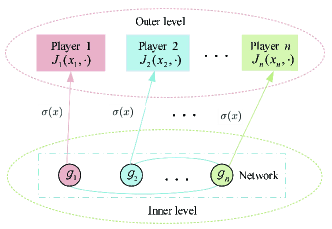
Figure 1: AG with bilevel structures.

Remark 1

In (1), if $J_{i}(x_{i},\sigma(x))=c$ and $x_{i}=d_{i}$ for some constant $c,~d_{i}\in\mathbb{R}$, (1) is reduced to be a distributed optimization problem [32]-[37]. While if letting $g_{i}(x_{i},y)=\frac{\|y\|^{2}}{2n}-\langle y,\sigma_{i}(x_{i})\rangle$ for some $\sigma_{i}(\cdot):\mathbb{R}^{m_{1}}\rightarrow\mathbb{R}^{m_{2}}$, then we have $\sigma(x)=\sum_{i=1}^{n}\sigma_{i}(x_{i})$, accordingly, problem (1) becomes the AG with single-level structure [7], [9]-[18]. Hence, the distributed optimization problem and the traditional AG are two special cases of (1). Consequently, studying (1) benefits for establishing a unified research framework for these two problems. To the best of our knowledge, this is the first time to study the distributed AGs with bilevel structures as (1).

The solution concept of problem (1), that we are committed to searching, is the SE [19]-[22].

Definition 1

For problem (1), the action profile $(x^{*},y^{*})$, where $x^{*}=(x_{i}^{*},x_{-i}^{*})\in\Omega$, is called an SE if it satisfies $J_{i}(x_{i}^{*},\sigma(x^{*}))\leq J_{i}(x_{i},\sigma(x_{i},x_{-i}^{*}))$ and $\sum_{i=1}^{n}g_{i}(x_{i}^{*},y^{*})\leq\sum_{i=1}^{n}g_{i}(x_{i}^{*},y)$ for any $x_{i}\in\Omega_{i}$, $y\in\mathbb{R}^{m_{2}}$ and $i\in\mathcal{V}$.

By (1), we know that $y^{*}=\sigma(x^{*})$. To estimate the aggregation, each player exchanges local information with its neighbors through an undirected graph $\mathcal{G}(A)$, where $A=(a_{ij})_{n\times n}$ represents the weighted matrix. To ensure that the information of each player can flow to all others, the following connectivity assumption associated with the communication graph is made.

Assumption 1

$A\textbf{1}_{n}=\textbf{1}_{n}$, and $\mathcal{G}(A)$ is connected.

To guarantee the existence of the SE, we assume that $\Omega_{i}$ is nonempty, convex and compact in the following lemma.

Assumption 2

$\Omega_{i}$ is nonempty, convex and compact for any $i\in\mathcal{V}$, i.e., $\sup_{x_{i}\in\Omega_{i}}\|x_{i}\|\leq K$ for some $K>0$. (Thus, there exists some constants $K_{i},i=0,1,\cdots,3$ such that $\|\nabla_{2}J_{i}(x_{i},y)\|\leq K_{1}$, $\|\nabla_{2}g_{i}(x_{i},y)\|\leq K_{2}$, $\|\nabla_{21}g_{i}(x_{i},y)\|_{\mathbb{F}}\leq K_{3}$, $\|\nabla_{22}g_{i}(x_{i},$ $y)\|_{\mathbb{F}}\leq K_{0}$ for any $x_{i}\in\Omega_{i}$ and $y\in\mathbb{R}^{m_{2}}$ if $y$ is bounded).

Define the pseudo-gradient mapping ${F}(x)=col({\nabla_{{x_{i}}}}J_{i}(x_{i},$ $\sigma(x)))_{i\in\mathcal{V}}$, where $x=(x_{i},x_{-i})$. Moreover, based on Definition 1 and results in [19, 23], a sufficient and necessary condition associated with the SEs of AG with bilevel structures is provided.

Lemma 1 ([19, 23])

For game $\Gamma(\mathcal{V},\Omega,{J})$ with bilevel structures, if $\Omega$ is convex and compact, and $J_{i}$, $i\in\mathcal{V}$ is differentiable and convex with respect to $x_{i}$, then the SEs always exist. Moreover, $(x^{*},y^{*})$ is an SE if and only if for any $k>0$,

$$\left\{\begin{split}&x^{*}=P_{\Omega}[x^{*}-k{F}(x^{*})]=0\\ &\sum_{i=1}^{n}\nabla_{2}g_{i}(x_{i}^{*},y^{*})=0.\end{split}\right.$$ (2)

Based on Lemma 1, we know that under Assumption 2, the SE exists. In the following proposition, each component of ${F}(x)$ is provided.

Proposition 1

Given ${J}_{i}(\cdot,\cdot):\mathbb{R}^{m_{1}}\times\mathbb{R}^{m_{2}}\rightarrow\mathbb{R}$ and $g_{i}(\cdot,$ $\cdot):\mathbb{R}^{m_{1}}\times\mathbb{R}^{m_{2}}\rightarrow\mathbb{R}$ as (1),
(i) $\nabla_{x_{i}}\sigma(x)=-\nabla_{21}g_{i}(x_{i},\sigma(x))\left(\sum_{i=1}^{n}\nabla_{22}g_{i}(x_{i},\sigma(x))\right)^{-1}$;
(ii)${\nabla_{{x_{i}}}}J_{i}(x_{i},$ $\sigma(x))=\nabla_{1}J_{i}(x_{i},$ $\sigma(x))+\nabla_{x_{i}}\sigma(x)\nabla_{2}J_{i}(x_{i},$ $\sigma(x))$.

Proof 1

See Section V. A for details.

Due to the strong convexity of $g_{i}(x_{i}(t),\cdot)$ and the boundedness of $\nabla_{21}g_{i}(x_{i},\sigma(x))$, based on (i) in Proposition 1 and Assumption 2, there holds that $\nabla_{x_{i}}\sigma(x)$ is bounded, then it is not difficulty to verify that

$$\begin{split}\|\sigma(x)-\sigma(y)\|\leq\ell\|x-y\|,\forall~x,y\in\Omega\end{split}$$ (3)

where $\ell=\frac{K_{3}}{\sqrt{n}\mu}$.

Assumption 3

(Lipschitz continuity) $\nabla_{1}J_{i}(x,y)$, $\nabla_{2}J_{i}(x,$ $y)$, $\nabla_{2}g_{i}(x,y)$, $\nabla_{21}g_{i}(x,y)$ and $\nabla_{22}g_{i}(x,y)$, $i=1,\cdots,n$, are all $L$-Lipschitz continuous with respect to both the first argument and the second argument for any $x\in\Omega_{i}$ and $y\in\mathbb{R}^{m_{2}}$.

Under Assumption 3, we can conclude that $F(x)$ is $L_{0}$-Lipschitz continuous for any $x\in\Omega$.

Lemma 2

Under Assumptions 2 and 3, $F(x)$ is $L_{0}$-Lipschitz continuous for any $x\in\Omega$, where $L_{0}=nL(K_{2}(K_{3}$ $+\mu+K_{3}\ell+\mu\ell)+(K_{3}\mu+\mu^{2})(1+\ell))/\mu^{2}$.

Proof 2

See Section V. B for details.

Furthermore, to ensure the existence and uniqueness of the SE, we also need the assumption on the strong monotonicity of the pseudo-gradient.

Assumption 4

(Strong monotonicity) $\langle F(x)-F(y),x-y\rangle\geq\theta\|x-y\|^{2},~\forall x,y\in\Omega$ for some $\theta>0$;

Based on Assumption 4, the solution to (2) is unique. Accordingly, we know that the SE uniquely exists. In fact, the Lipschitz continuity and strong monotonicity of the pseudo-gradient $F(x)$ are commonly adopted in the study of games, even in the cases with single-structures [7], [9]-[18], [23]-[25].

Remark 2

In traditional AGs [7], [9]-[18], the aggregation is defined as $\sigma(x)=\sum_{i=1}^{n}\sigma_{i}(x_{i})$, where $\sigma_{i}(\cdot):\mathbb{R}^{m_{1}}\rightarrow\mathbb{R}^{m_{2}}$. It is easy to achieve that $\nabla_{x_{i}}\sigma(x)=\nabla_{x_{i}}\sigma_{i}(x_{i})$, so the components of $\nabla_{x_{i}}\sigma(x)$ are not coupled at all, and the information of $\nabla_{x_{i}}\sigma_{i}(x_{i})$ is available to player $i$. However, based on Proposition 1, we have

$$\begin{split}&{\nabla_{{x_{i}}}}J_{i}(x_{i},\sigma(x))=\nabla_{1}J_{i}(x_{i},\sigma(x))-\nabla_{21}g_{i}(x_{i},\\ &\sigma(x))\left(\sum_{i=1}^{n}\nabla_{22}g_{i}(x_{i},\sigma(x))\right)^{-1}\nabla_{2}J_{i}(x_{i},\sigma(x)).\end{split}$$ (4)

In (4), $\sigma(x)$ is determined by the distributed optimization problem in the inner level of (1), and it can not be directly accessed. Moreover, all ${\nabla_{{x_{i}}}}J_{i}(x_{i},\sigma(x))$ and all $\nabla_{x_{i}}\sigma(x)$, $i=1,\cdots,n$ are coupled through the common term $\left(\sum_{i=1}^{n}\nabla_{22}g_{i}(x_{i},\sigma(x))\right)^{-1}$, which can not be directly accessed by the players. When making decisions, how to estimate the value of ${\nabla_{{x_{i}}}}J_{i}$ for players only using local information is a challenging problem. This problem formulation is rather different from the cases studied in [21]-[22] where the information of ${\nabla_{{x_{i}}}}J_{i}$ is assumed to be known by player $i$.

III Distributed methods involving second order gradient information

III-A Algorithm design

Denote the action of player $i$ at any time $t\geq 0$ by $x_{i,t}\in\mathbb{R}^{m_{1}}$, where $i\in\mathcal{V}$. To estimate $\sigma(x_{t})$ defined in the inner level of (1), it is necessary to solve the dynamical optimization problem $\min_{y\in\mathbb{R}^{m_{2}}}\sum_{i=1}^{n}g_{i}(x_{i,t},y)$, which is equivalent to the following optimization problem

$$\begin{split}&\min_{\tilde{y}\in\mathbb{R}^{nm_{2}}}g(x_{t},\tilde{y}),g(x_{t},\tilde{y})=\sum_{i=1}^{n}g_{i}(x_{i,t},y_{i})\\ &\emph{\emph{s. t. }}~~((I-A)\otimes I_{m_{2}})\tilde{y}=0\end{split}$$ (5)

where $\tilde{y}=col(y_{i})_{i=1,\cdots,n}$ and $y_{i}\in\mathbb{R}^{m_{2}}$. To address this problem, we propose the following primal-dual based distributed algorithm

$$\left\{\begin{split}y_{i,t+1}&=y_{i,t}+\kappa\Big{(}\sum_{j\in{\mathcal{N}_{i}}}a_{ij}\lambda_{j,t}-\lambda_{i,t}-\nabla_{2}g_{i}(x_{i,t},y_{i,t})\Big{)}\\ \lambda_{i,t+1}&=\lambda_{i,t}-\kappa\left(\sum_{j\in{\mathcal{N}_{i}}}a_{ij}y_{j,t+1}-y_{i,t+1}\right)\end{split}\right.$$ (6)

where $y_{i,t}\in\mathbb{R}^{m_{2}}$ represents the estimate on the aggregation $\sigma(x_{t})$, $\lambda_{i,t}\in\mathbb{R}^{m_{2}}$ is the dual variable, $\mathcal{N}_{i}$ is the neighbor set of player $i$, and $\kappa$ is a fixed step-size such that $0<\kappa<\min\Big{(}\frac{1}{L},$ $\frac{\mu}{(\lambda_{n}(I-A))^{2}}\Big{)}$. Moreover, based on (4), to compute ${\nabla_{{x_{i}}}}J_{i}(x_{i},\sigma(x))$, it is necessary to compute $\left(\sum_{i=1}^{n}\nabla_{22}g_{i}(x_{i,t},y_{i,t})\right)^{-1}\nabla_{2}J_{i}(x_{i,t},y_{i,t})$, which is a solution of the following optimization problem

$$\begin{split}&\min_{z_{i}\in\mathbb{R}^{m_{2}}}\frac{z_{i}^{T}\left(\sum_{j=1}^{n}\nabla_{22}g_{j}(x_{j,t},y_{j,t})\right)z_{i}}{2}+z_{i}^{T}\nabla_{2}J_{i}(x_{i,t},y_{i,t}).\end{split}$$ (7)

So estimating the term $\left(\sum_{j=1}^{n}\nabla_{22}g_{j}(x_{j,t},y_{j,t})\right)^{-1}\nabla_{2}J_{i}(x_{i,t},$ $y_{i,t})$ is equivalent to solving (7). It is not difficult to verify that the gradient of objective function in (7) is $(\sum_{j=1}^{n}\nabla_{22}g_{j}(x_{j,t},y_{j,t}))z_{i}+\nabla_{2}J_{i}(x_{i,t},y_{i,t})$, where the second order gradient information associated with $g_{i}$ is involved. To estimate $(\sum_{j=1}^{n}\nabla_{22}g_{j}(x_{j,t},$ $y_{j,t}))^{-1}\nabla_{2}J_{i}(x_{i,t},y_{i,t})$, we can first employe distributed average tracking algorithm (8) to track $\sum_{j=1}^{n}\nabla_{22}g_{j}(x_{j,t},y_{j,t})$, and then use the gradient descent algorithm (9) to solve (7). Now we propose the SOGD algorithm to handle problem (1) as follows.

 

Algorithm 1: SOGD algorithm
  • Initialization: At each iteration time $t\geq 0$, each player $i$ for any $i\in\mathcal{V}$ maintains its action $x_{i,t}\in\mathbb{R}^{m_{1}}$, the estimate $y_{i,t}\in\mathbb{R}^{m_{2}}$ on the aggregation $\sigma(x_{t})$, the estimate $v_{i,t}\in\mathbb{R}^{m_{2}\times m_{2}}$ on the average of $\nabla_{22}g_{i}(\cdot,\cdot)$, and the estimate $z_{i,t}\in\mathbb{R}^{m_{2}}$ on $-\left(\sum_{i=1}^{n}\nabla_{22}g_{i}(x_{i},\sigma(x))\right)^{-1}\nabla_{2}J_{i}(x_{i},$ $\sigma(x))$. Set the initial values as $x_{i,0}\in\Omega_{i}$, $y_{i,0}\in\mathbb{R}^{m_{2}}$, $\lambda_{i,0}=0$, $z_{i,0}\in\mathbb{R}^{m_{2}}$, $v_{i,0}=\nabla_{22}g_{i}(x_{i,0},y_{i,0})$.
• Iteration: For $t=0,1,2,\cdots$, each player $i$ updates variables using the following rules.

Step 1. Update variables $y_{i,t}$ and $\lambda_{i,t}$ in the inner level as (6).

Step 2. Update $v_{i,t}$ by the following distributed average tracking algorithm

$$\begin{split}v_{i,t+1}=&\sum_{j\in{\mathcal{N}_{i}}}a_{ij}v_{j,t}+\nabla_{22}g_{i}(x_{i,t+1},y_{i,t+1})\\ &-\nabla_{22}g_{i}(x_{i,t},y_{i,t}).\end{split}$$ (8)

Step 3. Update $z_{i,t}$ by the following gradient descent algorithm

$$\begin{split}&z_{i,t+1}=z_{i,t}-\alpha(nv_{i,t}z_{i,t}+\nabla_{2}J_{i}(x_{i,t},y_{i,t}))\\ \end{split}$$ (9)

where $\alpha$ is a fixed step-size such that $0<\alpha<\frac{\mu}{2nK_{0}^{2}}$.

Step 4. Update action $x_{i,t}$ in the outer level by the following projected gradient strategy

$$\left\{\begin{split}&x_{i,t+1}=(1-\eta_{t})x_{i,t}+\eta_{t}P_{\Omega_{i}}\big{[}x_{i,t}-k\hat{F}_{i,t}\big{]}\\ &\hat{F}_{i,t}=\nabla_{1}J_{i}(x_{i,t},y_{i,t})+\nabla_{21}g_{i}(x_{i,t},y_{i,t})z_{i,t}\end{split}\right.$$ (10)

where $\eta_{t}$ is a nonincreasing step-size such that $0\leq\eta_{t}\leq 1$, and $\frac{\theta}{L_{0}}>k>0$ is constant.
 

Note that each player $i$ updates its action only using local action information received from its neighbors, its own action set $\Omega_{i}$, and the information associated with a local bifunction $g_{i}$ in the inner level and its own cost function $J_{i}$ in the outer level. Thus, Algorithm 1 is distributed.

Remark 3

In Algorithm 1, the design of dynamics (6) is motivated by the primal-dual algorithms in [26]-[28]. The design of dynamics (8) is motivated by distributed average tracking algorithm [34, 35], as well as the consensus algorithms [29, 30]. Different from [26]-[28] where the static optimization problems are studied, both the problems (5) and (7) are dynamical optimization problems due to the influences of the actions $x_{i,t}$ and $y_{i,t}$, $i\in\mathcal{V}$. So the convergence of (6), (8) and (9) relies on the actions $x_{i,t}$, $i\in\mathcal{V}$ of the players. If the value of $x_{i,t}$ changes fast, then (6), (8) and (9) could not converge. To reduce the fluctuation of $x_{i,t}$, the projected gradient strategy involving the Krasnoselskii-Mann iterative strategy is proposed in (10).

III-B Convergence results

For simplicity, we denote

$$\begin{split}B=I-A.\end{split}$$ (11)

Note that if the graph is connected, then $B$ has a simple zero-eigenvalue, and the others are all positive [29]-[31]. The eigenvalues can be presented in ascending order: $0=\lambda_{1}(B)<\lambda_{2}(B)\leq\lambda_{3}(B)\leq\cdots\leq\lambda_{n}(B)$. For (5), the Lagrangian function can be defined as

$$L^{t}(\tilde{y},\lambda)=g(x_{t},\tilde{y})+\lambda^{T}(B\otimes I_{m_{2}})\tilde{y}.$$

Based on the Karush-Kuhn-Tucker (KKT) condition [38], for any $t\geq 0$, $y^{*}_{t}=\left[\sigma^{T}(x_{t}),\cdots,\sigma^{T}(x_{t})\right]^{T}$ is the solution of (5) if and only if

$$\left\{\begin{split}&\nabla_{2}g(x_{t},{y}^{*}_{t})+(B\otimes I_{m_{2}})\lambda^{*}_{t}=0\\ &(B\otimes I_{m_{2}}){y}^{*}_{t}=0\end{split}\right.$$ (12)

for some $\lambda^{*}_{t}=col(\lambda^{*}_{i,t})_{i=1,\cdots,n}$. In the following lemma, we establish the relationship between the variation in sequence $\{\lambda^{*}_{t}\}_{t=0,1,\cdots}$ and that in sequence $\{\nabla_{2}g(x_{t},{y}^{*}_{t})\}_{t=0,1,\cdots}$.

Lemma 3

Under Assumption 1, there exists a solution sequence $\{\lambda^{*}_{t}\}_{t=0,1,\cdots}$ to (12) satisfying
(i)$\|(B\otimes I_{m_{2}})(\lambda^{*}_{t}-\lambda)\|\geq\lambda_{2}(B)\|\lambda^{*}_{t}-\lambda\|$ for any $\lambda\in Null(\textbf{1}_{n}^{T}\otimes I_{m_{2}})$,
(ii)$\|\lambda^{*}_{t+1}-\lambda^{*}_{t}\|\leq\frac{1}{\lambda_{2}(B)}\|\nabla_{2}g(x_{t+1},{y}^{*}_{t+1})-\nabla_{2}g(x_{t},{y}^{*}_{t})\|$,
where $B$ is defined in (11).

Proof 3

See Section V. C for details.

Then, by (6) and (10), the estimate error between ${y}_{i,t}$ and the aggregation $\sigma(x_{t})$ is provided, refer to the following lemma for details.

Lemma 4

Under Assumptions 1-3, by (6) and (10), for some $0<\gamma<1$,

$$\begin{split}\|y_{i,t}-\sigma(x_{t})\|\leq\mathcal{O}\left(\gamma^{t}+\sum_{k=1}^{t}\gamma^{t-k}\eta_{k-1}\right),~~i\in\mathcal{V}.\\ \end{split}$$ (13)

Proof 4

See Section V. D for details.

Based on Lemma 4, by Assumption 2, we know that $y_{i}(t)$ is bounded. Moreover, if $\lim_{t\rightarrow\infty}\eta_{t}=0$, then $y_{i,t}$ converges to $\sigma(x_{t})$ for any $i\in\mathcal{V}$. Thus, the aggregation is estimated by all players. Particularly, based on the proof of Lemma 4, we know that the bound of $\|y_{i,t}-\sigma(x_{t})\|$ is influenced by the variation of actions, i.e., $\|x_{i,t+1}-x_{i,t}\|$, which results in the term $\sum_{k=1}^{t}\gamma^{t-k}\eta_{k-1}$ in (13) by using (10). By (13), we know that $y_{i,t}$ is bounded for any $t\geq 0$. Next, we will provide the estimate error of $v_{i,t}$ on the average of Hassian matrices $\nabla_{22}g_{i}(x_{i,t},y_{i,t})$, $i\in\mathcal{V}$.

Lemma 5

Under Assumptions 1-3, for some $0<\tau<1$,

$$\begin{split}\|v_{i,t}-\bar{G}_{t}\|_{\mathbb{F}}&\leq\mathcal{O}\Big{(}\sum_{k=0}^{t}\tau^{t-k}\eta_{k}+(t+1)\tau^{t}\\ &~~~~+\sum_{k=0}^{t}\tau^{t-k}\sum_{s=0}^{k}\tau^{k-s}\eta_{s}\Big{)},~~i\in\mathcal{V}\end{split}$$

where $\bar{G}_{t}=\frac{\sum_{i=1}^{n}\nabla_{22}g_{i}(x_{i,t},y_{i,t})}{n}$.

Proof 5

See Section V. E for details.

In what follows, a preliminary result on the error between the estimate $z_{i,t}$ and the real value $-(\sum_{i=1}^{n}\nabla_{22}g_{i}(x_{i,t},$ $\sigma(x_{t})))^{-1}\nabla_{2}J_{i}(x_{i,t},\sigma(x_{t}))$ will be provided.

Lemma 6

Under Assumptions 1-3, for any $i\in\mathcal{V}$,

$$\begin{split}&\|z_{i,t+1}-h_{i,t+1}\|\\ &\leq\Big{(}\vartheta+r_{1}\|\bar{G}_{t}-v_{i,t}\|_{\mathbb{F}}\Big{)}\|z_{i,t}-h_{i,t}\|\\ &~~~+\frac{4LK\ell\eta_{t}}{\mu}+r_{2}\|\bar{G}_{t}-v_{i,t}\|_{\mathbb{F}}\\ &~~~+r_{3}\Big{(}2+\vartheta+r_{1}\|\bar{G}_{t}-v_{i,t}\|_{\mathbb{F}}\Big{)}\sum_{i=1}^{n}\|y_{i,t}-\sigma(x_{t})\|\\ \end{split}$$ (14)

where $h_{i,t}=-\left(\sum_{i=1}^{n}\nabla_{22}g_{i}(x_{i,t},\sigma(x_{t}))\right)^{-1}\nabla_{2}J_{i}(x_{i,t},\sigma(x_{t}))$, $\vartheta=\sqrt{1-{n\mu\alpha}+2n^{2}K_{0}^{2}\alpha^{2}}<1$, $r_{1}=\sqrt{\frac{2\alpha n}{\mu}+4n^{2}\alpha^{2}}$, $r_{2}=$ $\sqrt{\frac{2\alpha K_{1}^{2}}{n\mu^{3}}+\frac{4K_{1}^{2}}{\mu^{2}}}$, and $r_{3}=\frac{nK_{1}L}{\mu^{2}}+\frac{nL}{\mu}$.

Proof 6

See Section V. F for details.

Now we present the convergence result on Algorithm 1 in the following theorem.

Theorem 1

Under Assumptions 1-4, if $\eta_{t}=\frac{b}{t+a}$ for some $a>\max(2k(\theta-kL_{0})b,b)$ and $b\geq\max\left(\frac{1}{2k(\theta-kL_{0})},1\right)$, then by Algorithm 1, both $\|x_{t}-x^{*}\|$ and $\|y_{i,t}-\sigma(x^{*})\|$, $\forall~i\in\mathcal{V}$ converge to zero with the convergence rate $\mathcal{O}(\sqrt{\ln t/t})$.

Proof 7

See Section V. G for details.

Remark 4

Based on Theorem 1, we know that the convergence rate of Algorithm 1 follows $\mathcal{O}(\sqrt{\ln t/t})$, which is faster than the common convergence rate $\mathcal{O}(\ln t/\sqrt{t})$ of distributed optimization algorithms with decaying step-size [32, 33]. Although the Krasnoselskii-Mann iterative strategy in (15) slows the convergence rate of the projected gradient algorithm, the fixed step-sizes $\alpha,\kappa$ and $k$ help to improve the convergence rate of the whole algorithm.

IV Distributed methods involving first order gradient information

Note that when running Algorithm 1, it is necessary to compute the Hassian matrix (second order gradient information) of the objective functions in the inner level. While in this section, distributed methods only using the first order gradient information will be proposed.

IV-A Algorithm design

For any $t\geq 0$ and $i\in\mathcal{V}$, consider the following optimization problem

$$\begin{split}y_{i}(\delta_{i},x_{t})=\arg\min_{y_{i}}\delta_{i}J_{i}(x_{i,t},y_{i})+\sum_{j=1}^{n}g_{j}(x_{j,t},y_{i})\end{split}$$ (15)

where $\delta_{i}>0$.

Assumption 5

For any $x_{i}\in\Omega_{i}$ and $i\in\mathcal{V}$, $J_{i}(x_{i},\cdot)$ is convex. Moreover, $\|\nabla_{22}J_{i}(x_{i},y_{i})\|_{\mathbb{F}}\leq\hbar$ for some $\hbar>0$.

Since in game $\Gamma(\mathcal{V},\Omega,{J})$, each player’s cost is determined by the aggregation $\sigma(x)$, then $J_{i}$ may not be convex with respect to $x_{-i}$ under Assumption 5. Moreover, by the strong convexity of $g_{i}(x_{i,t},\cdot)$, and using Assumption 5, we know that $\delta_{i}J_{i}(x_{i,t},y_{i})+\sum_{j=1}^{n}g_{j}(x_{j,t},y_{i})$ is $\mu-$strongly convex with respect to the second argument. Accordingly, $y_{i,t}(\delta_{i},x_{t})$ is the unique solution of (15). Due to the differences of $y_{i}(\delta_{i},x_{t})$ from $y_{k}(\delta_{i},x_{t})$ for any $i,k\in\mathcal{V}$, here we employ $w_{ik,t}\in\mathbb{R}^{m_{2}}$ to represent the estimate of player $k$ on $y_{i}(\delta_{i},x_{t})$. Based on (6), to estimate $y_{i}(\delta_{i},x_{t})$ for each player, the following distributed primal-dual algorithm is proposed

$$\left\{\begin{split}&w_{ik,t+1}=w_{ik,t}+\beta_{i}\Big{(}\sum_{j\in{\mathcal{N}_{k}}}a_{kj}u_{ij,t}-u_{ik,t}\\ &~~~~~~-\nabla_{2}g_{k}(x_{k,t},w_{ik,t})-c_{ki}\delta_{i}\nabla_{2}J_{i}(x_{i,t},w_{ii,t})\Big{)}\\ &u_{ik,t+1}=\lambda_{i,t}-\beta_{i}\Big{(}\sum_{j\in{\mathcal{N}_{k}}}a_{kj}w_{ij,t+1}-w_{ik,t+1}\Big{)}\end{split}\right.$$ (16)

where $c_{ki}=1$ if $i=k$, $c_{ki}=0$ otherwise, $u_{ik,t}\in\mathbb{R}^{m_{2}}$ is the dual variable with initial value $u_{ik,0}=0$, and $\beta_{i}>0$ is the step-size. To handle problem (1), now we propose the FOGD algorithm as follows.
  Algorithm 2: FOGD algorithm
  • Initialization: At each iteration time $t\geq 0$, each player $i$ for any $i\in\mathcal{V}$ maintains its action $x_{i,t}\in\mathbb{R}^{m_{1}}$, the estimate $y_{i,t}\in\mathbb{R}^{m_{2}}$ on $\sigma(x_{t})$ on the aggregation, and the estimate $w_{ik,t}$ on $y_{i}(\delta_{i},x_{t})$. Set the initial values as $x_{i,0}$ $\in\Omega_{i}$, $y_{i,0}\in\mathbb{R}^{m_{2}}$, $w_{i,0}\in\mathbb{R}^{m_{2}}$.
• Iteration: For $t=0,1,2,\cdots$, each player $i$ updates variables using the following rules.

Step 1. Update variables $y_{i,t}$ and $\lambda_{i,t}$ in the inner level as (6).

Step 2.  Update $w_{ik,t}$ as (16) with $0<\beta_{i}<\min\Big{(}\frac{1}{L+\hbar\delta_{i}},$ $\frac{\mu}{(\lambda_{n}(I-A))^{2}}\Big{)}$.

Step 3.  Compute the estimate on the gradient

$$\left\{\begin{split}&\hat{F}_{i,t}=\nabla_{1}J_{i}(x_{i,t},y_{i,t})+d_{i,t}\\ &d_{i,t}=\frac{\nabla_{2}g_{i}(x_{i,t},w_{ii,t})-\nabla_{2}g_{i}(x_{i,t},y_{i,t})}{\delta_{i}}\end{split}\right.$$ (17)

where $\delta_{i}>0$ is the estimate parameter.

Step 4. Update action $x_{i,t}$ in the outer level by the following projected gradient strategy

$$\begin{split}&x_{i,t+1}=(1-\eta_{t})x_{i,t}+\eta_{t}P_{\Omega_{i}}\big{[}x_{i,t}-k\hat{F}_{i,t}\big{]}\\ \end{split}$$ (18)

where $\eta_{t}$ is a nonincreasing step-size such that $0\leq\eta_{t}\leq 1$, and $\frac{\theta}{L_{0}}>k>0$ is constant.
 

In Algorithm 2, we use $d_{i,t}$ to estimate $\nabla_{x_{i}}\sigma(x_{t})\nabla_{2}J_{i}(x_{i,t},$ $\sigma(x_{t}))$ by the two-point estimate strategy (17). By Algorithm 2, the Hassian matrix information of the objective functions in the inner level are not required any more. Thus, Algorithm 2 is applicable to practical applications where computing the second order gradient information is rather expensive or impossible.

IV-B Convergence results

In this section, we will provide the convergence analysis of Algorithm 2. First, we introduce a new variable defined as

$$\begin{split}D_{i,t}=\frac{\nabla_{2}g_{i}(x_{i,t},y_{i}(\delta_{i},x_{t}))-\nabla_{2}g_{i}(x_{i,t},\sigma(x_{t}))}{\delta_{i}}.\end{split}$$ (19)

where $i\in\mathcal{V}$. In the next lemma, the relationship between $D_{i,t}$ and $\nabla_{x_{i}}\sigma(x_{t})\nabla_{2}J_{i}(x_{i,t},\sigma(x_{t}))$ is established.

Lemma 7

Under Assumptions 2, 3 and 5, for any $\delta_{i}>0$ and $i\in\mathcal{V}$,

$$\begin{split}\|D_{i,t}-\nabla_{x_{i}}\sigma(x_{t})\nabla_{2}J_{i}(x_{i,t},\sigma(x_{t}))\|\leq\mathcal{C}\delta_{i}\end{split}$$

where $\mathcal{C}=\frac{LK_{1}^{2}}{2n\mu^{2}}+\frac{\mathcal{C}_{0}K_{2}}{2}$, $\mathcal{C}_{0}=\frac{\sqrt{n}K_{1}^{2}L(1+\hbar)+\sqrt{n}\mu K_{1}L}{\mu^{3}}$, and $D_{i,t}$ is defined in $(\ref{eq113001})$.

Proof 8

See Section V. H for details.

Note that if $w_{ii,t}$ and $y_{i,t}$ approach to $y_{i}(\delta_{i},x_{t})$ and $\sigma(x_{t})$, respectively, then $d_{i,t}$ approximates $D_{i,t}$. Based on Lemma 7, we can conclude that the estimate error is linear with the estimate parameter $\delta_{i}$. With the help of the lemmas above, now we provide the convergence result on Algorithm 2.

Theorem 2

Under Assumptions 1-5, if $\eta_{t}=\frac{b}{t+a}$ for some $a>\max(2k(\theta-kL_{0})b,b)$ and $b\geq\max\left(\frac{1}{2k(\theta-kL_{0})},1\right)$, then by Algorithm 2, for any $\forall~i\in\mathcal{V}$,

$$\begin{split}\|x_{t}-x^{*}\|\leq\mathcal{O}\left(\sqrt{\ln t/{t}}+\sum_{i=1}^{n}(\sqrt{\mathcal{C}\delta_{i}}+\mathcal{C}\delta_{i})\right)\end{split}$$ (20)

and

$$\begin{split}\|y_{t}-\sigma(x^{*})\|\leq\mathcal{O}\left(\sqrt{\ln t/{t}}+\sum_{i=1}^{n}(\sqrt{\mathcal{C}\delta_{i}}+\mathcal{C}\delta_{i})\right)\end{split}$$ (21)

where $\mathcal{C}$ is defined in Lemma 7.

Proof 9

See Section V. I for details.

Remark 5

In (20) and (21), the term $\sqrt{\mathcal{C}\delta_{i}}+\mathcal{C}\delta_{i}$ comes from the estimate errors of $d_{i,t}$ defined in (17) on the value of $\nabla_{x_{i}}\sigma(x_{t})\nabla_{2}J_{i}(x_{i,t},\sigma(x_{t}))$. Particularly, if we set $\delta_{i}=\mathcal{O}(1/t)$, then we can achieve that $\|x_{t}-x^{*}\|\leq\mathcal{O}(\sqrt{\ln t/{t}})$ and $\|y_{t}-\sigma(x^{*})\|\leq\mathcal{O}(\sqrt{\ln t/{t}})$. So the same convergence rate as that of Algorithm 1 can be achieved.

V Mathematical proofs

In this section, we will provide the proofs of our results in detail. First, let us begin with presenting the proof of Proposition 1.

V-A Proof of Proposition 1

(i) By the fact that

$$\sigma(x)=\arg\min_{y}\sum_{i=1}^{n}g_{i}(x_{i},y),$$

there holds that $\sum_{i=1}^{n}\nabla_{2}g_{i}(x_{i},\sigma(x))=0$. Then taking the Jacobian matrix with respect to $x_{i}$ and using the chain derivative rule yield

$$\begin{split}\nabla_{21}g_{i}(x_{i},\sigma(x))+\nabla_{x_{i}}\sigma(x)\sum_{i=1}^{n}\nabla_{22}g_{i}(x_{i},\sigma(x))=0.\end{split}$$ (22)

Since $\sum_{i=1}^{n}g_{i}(x_{i},\sigma(x))$ is strongly convex, then we know that $\sum_{i=1}^{n}\nabla_{22}g_{i}(x_{i},\sigma(x))$ is positive definite. Accordingly, (22) implies (i).

(ii) Using the chain derivative rule, we have

$${\nabla_{{x_{i}}}}J_{i}(x_{i},\sigma(x))=\nabla_{1}J_{i}(x_{i},\sigma(x))+\nabla_{x_{i}}\sigma(x)\nabla_{2}J_{i}(x_{i},\sigma(x)).$$

Hence, the validity of (ii) is verified. $\blacksquare$

V-B Proof of Lemma 2

Using Assumption 2 and the strong convexity of $g_{i}$ to (i) in proposition 1, we know that $\|\nabla_{x_{i}}\sigma(x)\|_{\mathbb{F}}\leq\ell$ for any $x,y\in\Omega$. Moreover, by the continuity of $\sigma(\cdot)$, there holds that $\sigma(x)$ and $\sigma(y)$ are bounded for any $x,y\in\Omega$. Then, we have

$$\begin{split}&\|\nabla_{x_{i}}\sigma(x)-\nabla_{x_{i}}\sigma(y)\|_{\mathbb{F}}\\ &=\Big{\|}\nabla_{21}g_{i}(x_{i},\sigma(x))\Big{(}\sum_{i=1}^{n}\nabla_{22}g_{i}(x_{i},\sigma(x))\Big{)}^{-1}-\\ &~~~\nabla_{21}g_{i}(y_{i},\sigma(y))\Big{(}\sum_{i=1}^{n}\nabla_{22}g_{i}(y_{i},\sigma(y))\Big{)}^{-1}\Big{\|}_{\mathbb{F}}\\ &\leq K_{3}\Big{\|}\Big{(}\sum_{i=1}^{n}\nabla_{22}g_{i}(x_{i},\sigma(x))\Big{)}^{-1}\Big{\|}_{\mathbb{F}}\Big{\|}\sum_{i=1}^{n}\nabla_{22}g_{i}(x_{i},\sigma(x))\\ &~~~-\sum_{i=1}^{n}\nabla_{22}g_{i}(y_{i},\sigma(y))\Big{\|}_{\mathbb{F}}\Big{\|}\Big{(}\sum_{i=1}^{n}\nabla_{22}g_{i}(y_{i},\sigma(y))\Big{)}^{-1}\Big{\|}_{\mathbb{F}}\\ &~~~+\Big{\|}\Big{(}\sum_{i=1}^{n}\nabla_{22}g_{i}(y_{i},\sigma(y))\Big{)}^{-1}\Big{\|}_{\mathbb{F}}\|\nabla_{21}g_{i}(x_{i},\sigma(x))\\ &~~~-\nabla_{21}g_{i}(y_{i},\sigma(y))\|_{\mathbb{F}}\\ &\leq\left(\frac{K_{3}L}{\sqrt{n}\mu^{2}}+\frac{L}{\mu}+\frac{K_{3}L\ell}{\mu^{2}}+\frac{L\ell}{\sqrt{n}\mu}\right)\|x-y\|.\\ \end{split}$$

Note that

$$\begin{split}&\|\nabla_{x_{i}}\sigma(x)\nabla_{2}J_{i}(x_{i},\sigma(x))-\nabla_{x_{i}}\sigma(y)\nabla_{2}J_{i}(y_{i},\sigma(y))\|\\ &\leq\|\nabla_{x_{i}}\sigma(x)\|_{\mathbb{F}}\|\nabla_{2}J_{i}(x_{i},\sigma(x))-\nabla_{2}J_{i}(y_{i},\sigma(y))\|\\ &~~~+\|\nabla_{x_{i}}\sigma(x)-\nabla_{x_{i}}\sigma(y)\|_{\mathbb{F}}\|\nabla_{2}J_{i}(y_{i},\sigma(y))\|\\ &\leq\frac{K_{3}}{\sqrt{n}\mu}\|\nabla_{2}J_{i}(x_{i},\sigma(x))-\nabla_{2}J_{i}(y_{i},\sigma(y))\|\\ &~~~+K_{2}\|\nabla_{x_{i}}\sigma(x)-\nabla_{x_{i}}\sigma(y)\|_{\mathbb{F}}\\ &\leq\frac{K_{3}}{\sqrt{n}\mu}(L+L\ell)\|x-y\|\\ &~~~+K_{2}\|\nabla_{x_{i}}\sigma(x)-\nabla_{x_{i}}\sigma(y)\|_{\mathbb{F}}\\ &\leq L_{1}\|x-y\|\end{split}$$ (23)

where $L_{1}=\frac{K_{2}L(K_{3}+\sqrt{n}\mu+\sqrt{n}K_{3}\ell+\mu\ell)+K_{3}\mu L(1+\ell)}{\sqrt{n}\mu^{2}}$. Moreover,

$$\begin{split}&\|\nabla_{1}J_{i}(x_{i},\sigma(x))-\nabla_{1}J_{i}(y_{i},\sigma(y))\|\\ &\leq(1+\ell)L\|x-y\|.\end{split}$$ (24)

Based on (23) and (24), we can achieve that

$$\begin{split}\|F(x)-F(y)\|&\leq\sum_{i=1}^{n}\|\nabla_{1}J_{i}(x_{i},\sigma(x))-\nabla_{1}J_{i}(y_{i},\sigma(y))\|\\ &~~~+\sum_{i=1}^{n}\|\nabla_{x_{i}}\sigma(x)\nabla_{2}J_{i}(x_{i},\sigma(x))\\ &~~~-\nabla_{x_{i}}\sigma(y)\nabla_{2}J_{i}(y_{i},\sigma(y))\|\\ &\leq L_{0}\|x-y\|.\end{split}$$

Hence, the validity of the result is verified. $\blacksquare$

V-C Proof of Lemma 3

(i) Note that for the linear equations in the first line of (12), there must exist a solution $\lambda^{*}_{t}$ belongs to the range space of $B\otimes I_{m_{2}}$, i.e., there exists some $v\in\mathbb{R}^{nm_{2}}$ such that $(B\otimes I_{m_{2}})v=\lambda^{*}_{t}$. Since $(\textbf{1}_{n}^{T}\otimes I_{m_{2}})(B\otimes I_{m_{2}})v=0$, then $\lambda^{*}_{t}\in Null(\textbf{1}_{n}^{T}\otimes I_{m_{2}})$. Together with the fact that $\lambda\in Null(\textbf{1}_{n}^{T}\otimes I_{m_{2}})$, we have $\lambda^{*}_{t}-\lambda\in Null(\textbf{1}_{n}^{T}\otimes I_{m_{2}})$, i.e., $(\textbf{1}_{n}^{T}\otimes I_{m_{2}})(\lambda^{*}_{t}-\lambda)=0$. Note that $\textbf{1}_{n}^{T}B=0$ and $B^{2}$ is symmetric, so there exists an orthogonal matrix $U=[\textbf{1}_{n}/\sqrt{n},U_{0}]^{T}$ satisfying

$$\begin{split}&(\lambda^{*}_{t}-\lambda)^{T}(B\otimes I_{m_{2}})^{2}(\lambda^{*}_{t}-\lambda)\\ &=(\lambda^{*}_{t}-\lambda)^{T}U\Lambda^{2}U^{T}(\lambda^{*}_{t}-\lambda)\\ &\geq(\lambda_{2}(B))^{2}(\lambda^{*}_{t}-\lambda)^{T}UU^{T}(\lambda^{*}_{t}-\lambda)\\ &=(\lambda_{2}(B))^{2}\|\lambda^{*}_{t}-\lambda\|^{2}\end{split}$$

where $\Lambda=diag\{0,\lambda_{2}(B),\cdots,\lambda_{n}(B)\}$. Thus, the validity of (i) is verified.

(ii) By the arbitrariness of $t\geq 0$, we have

$$\left\{\begin{split}&\nabla_{2}g(x_{t},{y}^{*}_{t})+(B\otimes I_{m_{2}})\lambda^{*}_{t}=0\\ &\nabla_{2}g(x_{t+1},{y}^{*}_{t+1})+(B\otimes I_{m_{2}})\lambda^{*}_{t+1}=0\end{split}\right.$$ (25)

By (25), there holds that

$$\|(B\otimes I_{m_{2}})(\lambda^{*}_{t+1}-\lambda^{*}_{t})\|=\|\nabla_{2}g(x_{t},{y}^{*}_{t})-\nabla_{2}g(x_{t+1},{y}^{*}_{t+1})\|.$$

Using (i) and letting $\lambda=\lambda^{*}_{t+1}$, it immediately leads to the validity of (ii). $\blacksquare$

V-D Proof of Lemma 4

Denote $y_{t}=col(y_{i,t})_{i\in\mathcal{V}}$, $\lambda_{t}=col(\lambda_{i,t})_{i\in\mathcal{V}}$, $y^{*}_{t}=\left[\sigma^{T}(x_{t}),\cdots,\sigma^{T}(x_{t})\right]^{T}$, and let $\lambda^{*}_{t}$ be defined in Lemma 3, by (6) in Algorithm 1 and KKT condition in (12), we have

$$\left\{\begin{split}&y_{t+1}-y^{*}_{t}=y_{t}-y^{*}_{t}-\kappa((B\otimes I_{m_{2}})(\lambda_{t}-\lambda^{*}_{t})\\ &~~~~~~~~~~~~~~~+\nabla_{2}g(x_{t},y_{t})-\nabla_{2}g(x_{t},y^{*}_{t}))\\ &\lambda_{t+1}-\lambda^{*}_{t}=\lambda_{t}-\lambda^{*}_{t}+\kappa((B\otimes I_{m_{2}})(y_{t+1}-y^{*}_{t})).\end{split}\right.$$ (26)

Taking the square at both sides of the equations in (26) yields that

$$\begin{split}&\|y_{t+1}-y^{*}_{t}\|^{2}\\ &=\|y_{t}-y^{*}_{t}-\kappa(\nabla_{2}g(x_{t},y_{t})-\nabla_{2}g(x_{t},y_{t}^{*}))\|^{2}\\ &~~~~-2\kappa\langle(B\otimes I_{m_{2}})(\lambda_{t}-\lambda_{t}^{*}),y_{t}-y^{*}_{t}\\ &~~~~-\kappa(\nabla_{2}g(x_{t},y_{t})-\nabla_{2}g(x_{t},y_{t}^{*}))\rangle\\ &~~~+\kappa^{2}\|(B\otimes I_{m_{2}})(\lambda_{t}-\lambda_{t}^{*})\|^{2}\end{split}$$ (27)

and

$$\begin{split}&\|\lambda_{t+1}-\lambda^{*}_{t}\|^{2}\\ &=\|\lambda_{t}-\lambda^{*}_{t}\|^{2}+\kappa^{2}\|(B\otimes I_{m_{2}})(y_{t+1}-y^{*}_{t})\|^{2}\\ &~~~~+2\kappa\langle\lambda_{t}-\lambda^{*}_{t},(B\otimes I_{m_{2}})(y_{t+1}-y^{*}_{t})\rangle\\ &=\|\lambda_{t}-\lambda^{*}_{t}\|^{2}+\kappa^{2}\|(B\otimes I_{m_{2}})(y_{t+1}-y^{*}_{t})\|^{2}\\ &~~~-2\kappa^{2}\|(B\otimes I_{m_{2}})(\lambda_{t}-\lambda^{*}_{t})\|^{2}+\\ &~~~2\kappa\langle(B\otimes I_{m_{2}})(\lambda_{t}-\lambda_{t}^{*}),y_{t}-y^{*}_{t}\\ &~~~-\kappa(\nabla_{2}g(x_{t},y_{t})-\nabla_{2}g(x_{t},y_{t}^{*}))\rangle.\end{split}$$ (28)

Combining (27) and (28) results in that

$$\begin{split}&\|y_{t+1}-y^{*}_{t}\|^{2}+\|\lambda_{t+1}-\lambda^{*}_{t}\|^{2}\\ &=\|y_{t}-y^{*}_{t}-\kappa(\nabla_{2}g(x_{t},y_{t})-\nabla_{2}g(x_{t},y_{t}^{*}))\|^{2}\\ &~~~+\kappa^{2}\|(B\otimes I_{m_{2}})(\lambda_{t}-\lambda_{t}^{*})\|^{2}+\|\lambda_{t}-\lambda^{*}_{t}\|^{2}\\ &~~~+\kappa^{2}\|(B\otimes I_{m_{2}})(y_{t+1}-y^{*}_{t})\|^{2}\\ &~~~-2\kappa^{2}\|(B\otimes I_{m_{2}})(\lambda_{t}-\lambda^{*}_{t})\|^{2}\\ \end{split}$$

$$\begin{split}&\leq\|y_{t}-y^{*}_{t}-\kappa(\nabla_{2}g(x_{t},y_{t})-\nabla_{2}g(x_{t},y_{t}^{*}))\|^{2}\\ &~~~+\kappa^{2}(\lambda_{n}(B))^{2}\|y_{t+1}-y^{*}_{t}\|^{2}\\ &~~~+(1-\kappa^{2}(\lambda_{2}(B))^{2})\|\lambda_{t}-\lambda^{*}_{t}\|^{2}\\ \end{split}$$ (29)

where the inequality holds by the fact that $\|B(\lambda_{t}-\lambda^{*}_{t})\|\leq\lambda_{n}(B)\|\lambda_{t}-\lambda^{*}_{t}\|^{2}$ and using (i) in Lemma 3. By (10), we know that $x_{i}(t)\in\Omega_{i}$ for any $i\in{\mathcal{V}}$. Using the Lipschitz continuity and the strong monotonicity of $\nabla_{2}g_{i}(\cdot,\cdot)$ with respect to the second argument yields that

$$\begin{split}&\|y_{t}-y^{*}_{t}-\kappa(\nabla_{2}g(x_{t},y_{t})-\nabla_{2}g(x_{t},y_{t}^{*}))\|^{2}\\ &\leq\|y_{t}-y^{*}_{t}\|^{2}+\kappa^{2}\|\nabla_{2}g(x_{t},y_{t})-\nabla_{2}g(x_{t},y_{t}^{*})\|^{2}\\ &~~~-2\kappa\langle y_{t}-y^{*}_{t},\nabla_{2}g(x_{t},y_{t})-\nabla_{2}g(x_{t},y_{t}^{*})\rangle\\ &\leq\|y_{t}-y^{*}_{t}\|^{2}+\kappa^{2}L\langle y_{t}-y^{*}_{t},\nabla_{2}g(x_{t},y_{t})-\nabla_{2}g(x_{t},y_{t}^{*})\rangle\\ &~~~-2\kappa\langle y_{t}-y^{*}_{t},\nabla_{2}g(x_{t},y_{t})-\nabla_{2}g(x_{t},y_{t}^{*})\rangle\\ &\leq\|y_{t}-y^{*}_{t}\|^{2}+(\kappa^{2}L-2\kappa)\mu\|y_{t}-y^{*}_{t}\|^{2}\\ &=(1-\kappa\mu(2-\eta_{y}L))\|y_{t}-y^{*}_{t}\|^{2}\\ &=(1-\kappa\mu(1-\eta_{y}L))\|y_{t}-y^{*}_{t}\|^{2}-\kappa\mu\|y_{t}-y^{*}_{t}\|^{2}\\ &=(1-\kappa\mu(1-\eta_{y}L))(1-\kappa^{2}(\lambda_{n}(B))^{2})\|y_{t}-y^{*}_{t}\|^{2}\\ &~~~-\kappa(\mu-\kappa(\lambda_{n}(B))^{2}(1-\kappa\mu(1-\eta_{y}L)))\|y_{t}-y^{*}_{t}\|^{2}\\ &\leq(1-\kappa\mu(1-\eta_{y}L))(1-\kappa^{2}(\lambda_{n}(B))^{2})\|y_{t}-y^{*}_{t}\|^{2}\\ \end{split}$$ (30)

where the last inequality is true due to the facts that $\kappa<\frac{1}{L}$ and $\kappa<\frac{\mu}{(\lambda_{n}(B))^{2}}$. From (29) and (30), it follows that

$$\begin{split}&(1-\kappa^{2}(\lambda_{n}(B))^{2})\|y_{t+1}-y^{*}_{t}\|^{2}+\|\lambda_{t+1}-\lambda^{*}_{t}\|^{2}\\ &\leq\gamma_{0}((1-\kappa^{2}(\lambda_{n}(B))^{2})\|y_{t}-y^{*}_{t}\|^{2}+\|\lambda_{t}-\lambda^{*}_{t}\|^{2})\\ \end{split}$$ (31)

where $\gamma_{0}=\max(1-\kappa\mu(1-\kappa L),1-\kappa^{2}(\lambda_{2}(B))^{2}))$. By the fact that $\mu/L\leq 1$, it is not difficult to verify that $\gamma_{0}\in[0,1)$. Letting $e_{t}=\left[\sqrt{1-\kappa^{2}(\lambda_{n}(B))^{2}}(y_{t}-y^{*}_{t})^{T},(\lambda_{t}-\lambda^{*}_{t})^{T}\right]^{T}$ and $\gamma=\sqrt{\gamma_{0}}$, by (31), we have

$$\begin{split}\|e_{t+1}\|\leq\gamma\|e_{t}\|+\|r_{t}\|\\ \end{split}$$ (32)

where $r_{t}=\Big{[}\sqrt{1-\kappa^{2}(\lambda_{n}(B))^{2}}(y_{t+1}^{*}-y^{*}_{t})^{T},(\lambda_{t+1}^{*}-$ $\lambda^{*}_{t})^{T}\Big{]}^{T}$. Using (ii) in Lemma 3 yields

$$\begin{split}\|\lambda^{*}_{t+1}-\lambda^{*}_{t}\|&\leq\frac{1}{\lambda_{2}(B)}\|\nabla_{2}g(x_{t+1},{y}^{*}_{t+1})-\nabla_{2}g(x_{t},{y}^{*}_{t})\|\\ &\leq\frac{L}{\lambda_{2}(B)}(\|x_{t+1}-x_{t}\|+\|{y}^{*}_{t+1}-{y}^{*}_{t}\|)\end{split}$$

where the second inequality holds by using the Lipschitz continuity of $\nabla_{2}g_{i}(\cdot,\cdot)$. Then letting $\varrho_{1}=\frac{L}{\lambda_{2}(B)}$ and $\varrho_{2}=\sqrt{1-\kappa^{2}(\lambda_{n}(B))^{2}}+\varrho_{1}$, it is easy to verify that

$$\begin{split}\|r_{t}\|&\leq\varrho_{1}\|x_{t+1}-x_{t}\|+\varrho_{2}\|{y}^{*}_{t+1}-{y}^{*}_{t}\|.\end{split}$$ (33)

Submitting (33) to (32) yields

$$\begin{split}\|e_{t+1}\|\leq\gamma\|e_{t}\|+\varrho_{1}\|x_{t+1}-x_{t}\|+\varrho_{2}\|{y}^{*}_{t+1}-{y}^{*}_{t}\|.\\ \end{split}$$ (34)

Due to the fact that $\sum_{i=1}^{n}g_{i}(x_{i},\sigma(x))$ is strongly convex, one knows that $\sum_{i=1}^{n}\nabla_{22}g_{i}(x_{i},\sigma(x))$ is bounded. By (3), there holds $\|{y}^{*}_{t+1}-{y}^{*}_{t}\|=\sqrt{n}\|\sigma(x_{t+1})-\sigma(x_{t})\|\leq\sqrt{n}\ell\|x_{t+1}-x_{t}\|$. Moreover, by (10), we have $\|x_{t+1}-x_{t}\|\leq 2\sqrt{n}K\eta_{t}$, where $K$ is defined in Assumption 2. By (34), letting $\varrho_{0}=2\sqrt{n}K(\varrho_{1}+\sqrt{n}\varrho_{1}\ell)$, we have

$$\begin{split}\|e_{t+1}\|\leq\gamma\|e_{t}\|+\varrho_{0}\eta_{t}.\\ \end{split}$$

It follows that $e_{t+1}\leq\gamma^{t}\|e_{0}\|+\varrho_{0}\sum_{k=1}^{t}\gamma^{t-k}\eta_{k-1}$, which immediately implies (13). Thus, the validity of the result is verified. $\blacksquare$

V-E Proof of Lemma 5

To prove Lemma 5, we present the following lemma.

Lemma 8 ([32])

Under Assumption 1, for any $i,j\in\mathcal{V}$,

$$\begin{split}\left|[A^{t}]_{ij}-\frac{1}{n}\right|\leq\sqrt{n}\rho^{t}\end{split}$$ (35)

where $\rho$ is the second largest eigenvalue of $A$ such that $0<\rho<1$.

Proof of Lemma 5. Denote $\bar{v}_{t}=\frac{1}{n}\sum_{i=1}^{n}v_{i,t}$, taking the average at both sides of (8) in Algorithm 1, we have $\bar{v}_{k+1}=\bar{v}_{k}+\bar{G}_{k+1}-\bar{G}_{k}$. Taking the summation with respect to $k=0,\cdots,t$ yields $\bar{v}_{t+1}-\bar{v}_{0}=\bar{G}_{t+1}-\bar{G}_{0}$. Due to the fact that $\bar{v}_{0}=\bar{G}_{0}$, there holds $\bar{v}_{t}=\bar{G}_{t}$. Moreover, denote ${v}_{t}=col(v_{i,t})_{i\in\mathcal{V}}$, $d_{i,t}=\nabla_{22}g_{i}(x_{i,t},y_{i,t})-\nabla_{22}g_{i}(x_{i,t-1},y_{i,t-1})$ and $d_{t}=col(d_{i,t})_{i\in\mathcal{V}}$, we have

$$\begin{split}v_{i,t}&=\sum_{j\in\mathcal{N}_{i}}a_{ij,t-1}v_{j,t-1}+d_{i,t}\\ &=\Big{(}[A]_{i\cdot}\otimes I_{m_{2}}\Big{)}v_{t-1}+d_{i,t}\\ &=\Big{(}[A^{t}]_{i\cdot}\otimes I_{m_{2}}\Big{)}v_{0}+\sum_{k=1}^{t}\Big{(}[A^{t-k}]_{i\cdot}\otimes I_{m_{2}}\Big{)}d_{k}.\end{split}$$ (36)

By the fact that $A^{t}$ is a doubly stochastic matrix, one has

$$\begin{split}\bar{v}_{t}=\Big{(}\frac{1}{n}\textbf{1}_{n}^{T}\otimes I_{m_{2}}\Big{)}v_{0}+\sum_{k=1}^{t}\Big{(}\frac{\textbf{1}}{n}1_{n}^{T}\otimes I_{m_{2}}\Big{)}d_{k}.\end{split}$$ (37)

Combining (36) and (37) results in that for any $i\in\mathcal{V}$,

$$\begin{split}&\|v_{i,t}-\bar{v}_{t}\|_{\mathbb{F}}\\ &\leq\left\|\left([A^{t}]_{i\cdot}-\frac{1}{n}{\textbf{1}}_{n}^{T}\right)\otimes I_{m_{2}}\right\|_{\mathbb{F}}\|v_{0}\|_{\mathbb{F}}\\ &~~~+\sum_{k=1}^{t}\left\|\left([A^{t}]_{i\cdot}-\frac{1}{n}{\textbf{1}}_{n}^{T}\right)\otimes I_{m_{2}}\right\|_{\mathbb{F}}\|d_{k}\|_{\mathbb{F}}.\end{split}$$ (38)

Note that

$$\begin{split}\|d_{t}\|_{\mathbb{F}}&\leq\sum_{i=1}^{n}\|\nabla_{22}g_{i}(x_{i,t},y_{i,t})-\nabla_{22}g_{i}(x_{i,t-1},y_{i,t-1})\|_{\mathbb{F}}\\ &\leq\sum_{i=1}^{n}\|\nabla_{22}g_{i}(x_{i,t},y_{i,t})-\nabla_{22}g_{i}(x_{i,t-1},y_{i,t})\|_{\mathbb{F}}\\ &~~~+\sum_{i=1}^{n}\|\nabla_{22}g_{i}(x_{i,t-1},y_{i,t})-\nabla_{22}g_{i}(x_{i,t-1},y_{i,t-1})\|_{\mathbb{F}}\\ &\leq\sum_{i=1}^{n}L\|x_{i,t}-x_{i,t-1}\|+\sum_{i=1}^{n}L\|{y}_{i,t}-{y}_{i,t-1}\|\\ &\leq 2nLK\eta_{t-1}+\sum_{i=1}^{n}L\|{y}_{i,t}-{y}_{i,t-1}\|\end{split}$$

where the last inequality results from (10) and the boundedness of $\Omega_{i}$ in Assumption 2. Moreover, by (3), we have $\|\sigma(x_{t})-\sigma(x_{t-1})\|\leq\ell\|x_{t}-x_{t-1}\|$. Then, for any $\in\mathcal{V}$,

$$\begin{split}&\|{y}_{i,t}-{y}_{i,t-1}\|\\ &=\|({y}_{i,t}-\sigma(x_{t}))+(\sigma(x_{t})-\sigma(x_{t-1}))\\ &~~~~+(\sigma(x_{t-1})-{y}_{i,t-1})\|\\ &\leq\|{y}_{i,t}-\sigma(x_{t})\|+\|\sigma(x_{t})-\sigma(x_{t-1})\|\\ &~~~+\|\sigma(x_{t-1})-{y}_{i,t-1}\|\\ &\leq\mathcal{O}\left(\gamma^{t}+\sum_{k=1}^{t}\gamma^{t-k}\eta_{k-1}+\ell\|\sigma(x_{t})-\sigma(x_{t-1})\|\right)\\ &\leq\mathcal{O}\left(\gamma^{t}+\sum_{k=1}^{t}\gamma^{t-k}\eta_{k-1}+2K\sqrt{n}\ell\eta_{t-1}\right)\end{split}$$

where the second inequality holds by using Lemma 4, and the last one results from (10) and the compactness of $\Omega_{i}$. Then,

$$\begin{split}\|d_{t}\|_{\mathbb{F}}&\leq 2nLK(1+\sqrt{n}\ell)\eta_{t-1}\\ &~~~+\frac{2n\rho L}{\gamma}\left(\gamma^{t}+\sum_{k=1}^{t}\gamma^{t-k}\eta_{k-1}\right).\end{split}$$ (39)

Submitting (39) to (38) and using Lemma 8 result in that

$$\begin{split}&\|v_{i,t}-\bar{v}_{t}\|_{\mathbb{F}}\\ &\leq\frac{2n^{2}LK(1+\sqrt{n}\ell)\sqrt{{m_{2}}}}{\rho}\sum_{k=0}^{t}\rho^{t-k}\eta_{k}\\ &~~~~+n\sqrt{{m_{2}}}\|v_{0}\|_{\mathbb{F}}\rho^{t}+\frac{2n^{2}L\rho\sqrt{{m_{2}}}}{\gamma\rho}\sum_{k=0}^{t}\rho^{t-k}\gamma^{k}\\ &~~~~+\frac{2n^{2}L\rho\sqrt{{m_{2}}}}{\gamma\rho}\sum_{k=0}^{t}\rho^{t-k}\sum_{s=0}^{k}\gamma^{k-s}\eta_{s}.\end{split}$$

Let $\tau=\max\left(\gamma,\rho\right)$, and recall the fact that $\bar{v}_{t}=\bar{G}_{t}$, it immediately leads to the validity of the result. $\blacksquare$

V-F Proof of Lemma 6

Denote $M_{t}=n\bar{G}_{t}$, since matrix $M_{t}$ is positive definite, then $z_{i,t}^{*}=-M_{t}^{-1}\nabla_{2}J_{i}(x_{i,t},y_{i,t})$ is the unique solution to equation $M_{t}z+\nabla_{2}J_{i}(x_{i,t},y_{i,t})=0$. Accordingly, $M_{t}z^{*}_{t}+\nabla_{2}J_{i}(x_{i,t},y_{i,t})=0$, $\forall~t\geq 0$ and $i\in\mathcal{V}$. By (9) in Algorithm 1, we have

$$\begin{split}&\|z_{i,t+1}-z_{i,t}^{*}\|^{2}\\ &=\|z_{i,t}-z_{i,t}^{*}-\alpha(nv_{i,t}z_{i,t}+\nabla_{2}J_{i}(x_{i,t},y_{i,t}))\|^{2}\\ &=\|z_{i,t}-z_{i,t}^{*}\|^{2}-2\alpha\langle z_{i,t}-z_{i,t}^{*},M_{t}z_{i,t}\\ &~~~+\nabla_{2}J_{i}(x_{i,t},y_{i,t})-(M_{t}z_{i,t}^{*}+\nabla_{2}J_{i}(x_{i,t},y_{i,t}))\rangle\\ &~~~+2\alpha\langle z_{i,t}-z_{i,t}^{*},M_{t}z_{i,t}-nv_{i,t}z_{i,t}\rangle\\ &~~~+\alpha^{2}\|nv_{i,t}z_{i,t}+\nabla_{2}J_{i}(x_{i,t},y_{i,t}))\\ &~~~-(M_{t}z_{i,t}^{*}+\nabla_{2}J_{i}(x_{i,t},y_{i,t}))\|^{2}\\ &=\|z_{i,t}-z_{i,t}^{*}\|^{2}-2\alpha\langle z_{i,t}-z_{i,t}^{*},M_{t}(z_{i,t}-z_{i,t}^{*})\rangle\\ &~~~+2\alpha\langle z_{i,t}-z_{i,t}^{*},M_{t}z_{i,t}-nv_{i,t}z_{i,t}\rangle\\ &~~~+\alpha^{2}\|nv_{i,t}z_{i,t}-M_{t}z_{i,t}^{*}\|^{2}\\ &\leq(1-2n\mu\alpha)\|z_{i,t}-z_{i,t}^{*}\|^{2}\\ &~~~+2\alpha\langle z_{i,t}-z_{i,t}^{*},M_{t}z_{i,t}-nv_{i,t}z_{i,t}\rangle\\ \end{split}$$

$$\begin{split}&~~~+\alpha^{2}\|nv_{i,t}z_{i,t}-M_{t}z_{i,t}^{*}\|^{2}\\ \end{split}$$ (40)

where the inequality holds true due to the strong monotonicity of $g_{i}(x_{i,t},\cdot)$. It is not difficult to verify that $\|z_{i,t}^{*}\|\leq\frac{K_{1}}{n\mu}$, then there holds

$$\begin{split}&\langle z_{i,t}-z_{i,t}^{*},M_{t}z_{i,t}-nv_{i,t}z_{i,t}\rangle\\ &\leq\|z_{i,t}-z_{i,t}^{*}\|\|(M_{t}-nv_{i,t})z_{i,t}\|\\ &\leq\frac{n\mu}{2}\|z_{i,t}-z_{i,t}^{*}\|^{2}+\frac{1}{2n\mu}\|(M_{t}-nv_{i,t})z_{i,t}\|^{2}\\ &\leq\frac{n\mu}{2}\|z_{i,t}-z_{i,t}^{*}\|^{2}+\frac{1}{n\mu}\|M_{t}-nv_{i,t}\|_{\mathbb{F}}^{2}\|z_{i,t}-z_{i,t}^{*}\|^{2}\\ &~~~+\frac{K_{1}^{2}}{n^{3}\mu^{3}}\|M_{t}-nv_{i,t}\|_{\mathbb{F}}^{2}\\ \end{split}$$ (41)

where the second inequality results by using the Young’s inequality theory, and the last one holds due to the fact that $\|u+v\|^{2}\leq 2\|u\|^{2}+2\|v\|^{2}$ for any vectors $u,v\in\mathbb{R}^{m_{2}}$. Moreover,

$$\begin{split}&\|nv_{i,t}z_{i,t}-M_{t}z_{i,t}^{*}\|^{2}\\ &=\|(nv_{i,t}z_{i,t}-M_{t}z_{i,t})+(M_{t}z_{i,t}-M_{t}z_{i,t}^{*})\|^{2}\\ &\leq 2\|nv_{i,t}-M_{t}\|_{\mathbb{F}}^{2}\|z_{i,t}\|^{2}+2\|M_{t}\|_{\mathbb{F}}^{2}\|z_{i,t}-z_{i,t}^{*}\|^{2}\\ &\leq 4\|nv_{i,t}-M_{t}\|_{\mathbb{F}}^{2}\|z_{i,t}-z_{i,t}^{*}\|^{2}+4\|z_{i,t}^{*}\|^{2}\|M_{t}-nv_{i,t}\|_{\mathbb{F}}^{2}\\ &~~~+2\|M_{t}\|_{\mathbb{F}}^{2}\|z_{i,t}-z_{i,t}^{*}\|^{2}\\ &\leq\left(4\|nv_{i,t}-M_{t}\|_{\mathbb{F}}^{2}+2n^{2}K_{0}^{2}\right)\|z_{i,t}-z_{i,t}^{*}\|^{2}\\ &~~~+\frac{4K_{1}^{2}}{n^{2}\mu^{2}}\|M_{t}-nv_{i,t}\|_{\mathbb{F}}^{2}\\ \end{split}$$ (42)

where the last inequality holds by using the boundedness of $\nabla_{22}g_{i}(x_{i,t},y_{i,t})$ in Assumption 2. Submitting (41) and (42) to (40), and using the fact that $M_{t}=n\bar{G}_{t}$, we have

$$\begin{split}\|z_{i,t+1}-z_{i,t}^{*}\|^{2}&\leq\Big{(}\vartheta^{2}+r_{1}^{2}\|\bar{G}_{t}-v_{i,t}\|_{\mathbb{F}}^{2}\Big{)}\|z_{i,t}-z_{i,t}^{*}\|^{2}\\ &~~~+r_{2}^{2}\|\bar{G}_{t}-v_{i,t}\|_{\mathbb{F}}^{2}.\\ \end{split}$$

Due to the fact that $0<\alpha<\frac{\mu}{2nK_{0}^{2}}$ and $\mu<K_{0}$, there holds that $0<1-{n\mu\alpha}+2n^{2}K_{0}^{2}\alpha^{2}<1$. Thus,

$$\begin{split}&\|z_{i,t+1}-h_{i,t+1}\|\\ &\leq\|z_{i,t+1}-z_{i,t}^{*}\|+\|h_{i,t+1}-h_{i,t}\|+\|z_{i,t}^{*}-h_{i,t}\|\\ &\leq\Big{(}\vartheta+r_{1}\|\bar{G}_{t}-v_{i,t}\|_{\mathbb{F}}\Big{)}\|z_{i,t}-h_{i,t}\|\\ &~~~+r_{2}\|\bar{G}_{t}-v_{i,t}\|_{\mathbb{F}}+\|h_{i,t+1}-h_{i,t}\|\\ &~~~+\Big{(}1+\vartheta+r_{1}\|\bar{G}_{t}-v_{i,t}\|_{\mathbb{F}}\Big{)}\|z_{i,t}^{*}-h_{i,t}\|.\\ \end{split}$$ (43)

Denote $H_{t}=\sum_{i=1}^{n}\nabla_{22}g_{i}(x_{i,t},\sigma(x_{t}))$, by the strong convexity of $\sum_{i=1}^{n}g_{i}(\cdot,\cdot)$ with respect to the second argument, one has $\|M_{t}^{-1}\|_{\mathbb{F}}\leq\frac{1}{\mu}$ and $\|H_{t}^{-1}\|_{\mathbb{F}}\leq\frac{1}{\mu}$. Furthermore,

$$\begin{split}&\|z_{i,t}^{*}-h_{i,t}\|\\ &=\|M_{t}^{-1}\nabla_{2}J_{i}(x_{i,t},y_{i,t})-H_{t}^{-1}\nabla_{2}J_{i}(x_{i,t},\sigma(x_{t}))\|\\ &=\|M_{t}^{-1}\nabla_{2}J_{i}(x_{i,t},y_{i,t})-H_{t}^{-1}\nabla_{2}J_{i}(x_{i,t},y_{i,t})\\ &~~~~+H_{t}^{-1}\nabla_{2}J_{i}(x_{i,t},y_{i,t})-H_{t}^{-1}\nabla_{2}J_{i}(x_{i,t},\sigma(x_{t}))\|\\ &\leq\|\nabla_{2}J_{i}(x_{i,t},y_{i,t})\|\|M_{t}^{-1}-H_{t}^{-1}\|_{\mathbb{F}}\\ \end{split}$$

$$\begin{split}&~~~~+\|H_{t}^{-1}\|_{\mathbb{F}}\|\nabla_{2}J_{i}(x_{i,t},y_{i,t})-\nabla_{2}J_{i}(x_{i,t},\sigma(x_{t}))\|\\ &\leq K_{1}\|M_{t}^{-1}(H_{t}-M_{t})H_{t}^{-1}\|+\frac{L}{\mu}\|y_{i,t}-\sigma(x_{t})\|\\ &\leq K_{1}\|M_{t}^{-1}\|_{\mathbb{F}}\|H_{t}-M_{t}\|_{\mathbb{F}}\|H_{t}^{-1}\|_{\mathbb{F}}\\ &~~~+\frac{L}{\mu}\|y_{i,t}-\sigma(x_{t})\|\\ &\leq r_{3}\sum_{i=1}^{n}\|y_{i,t}-\sigma(x_{t})\|\end{split}$$ (44)

where the second inequality is true due to the boundedness of $\nabla_{2}J_{i}$ in Assumption 2 and its Lipschitz continuity in Assumption 3, and the last one holds by the Lipschitz continuity of $\nabla_{22}g_{i}$. Similarly, we have

$$\begin{split}&\|h_{i,t+1}-h_{i,t}\|\\ &\leq\|\nabla_{2}J_{i}(x_{i,t+1},\sigma(x_{t+1}))\|\|H_{t+1}^{-1}-H_{t}^{-1}\|_{\mathbb{F}}\\ &~~~~+\|H_{t}^{-1}\|_{\mathbb{F}}\|\nabla_{2}J_{i}(x_{i,t+1},\sigma(x_{t+1}))-\nabla_{2}J_{i}(x_{i,t},\sigma(x_{t}))\|\\ &\leq K_{1}\|H_{t+1}^{-1}(H_{t}-H_{t+1}^{-1})H_{t}^{-1}\|+\frac{2L}{\mu}\|\sigma(x_{t+1})-\sigma(x_{t})\|\\ &\leq\frac{nK_{1}L}{\mu^{2}}\sum_{i=1}^{n}\|y_{i,t}-\sigma(x_{t})\|+\frac{2L\ell}{\mu}\|x_{t+1}-x_{t}\|.\\ \end{split}$$ (45)

Submitting (44) and (45) to (43), and using (10) immediately yield (14). Thus, the validity of the results is verified. $\blacksquare$

V-G Proof of Theorem 1

Before providing the proof of Theorem 1, the following two lemmas are necessary.

Lemma 9

Given a nonnegative sequence $\{\xi_{t}\}_{t=0,1,\cdots}$ such that

$$\begin{split}\xi_{t+1}\leq\Big{(}1-\frac{b_{1}}{t+a}\Big{)}\xi_{t}+\frac{b_{2}}{(t+a)^{2}}+b_{3}c^{t}+\frac{b_{4}}{t+a}\end{split}$$

for some $b_{i}>0$, $i=1,\cdots,4$, if $b_{1}\geq 1$, $a>b_{1}$ and $0<c<1$, then for any $t\geq 0$,

$$\begin{split}\xi_{t}&\leq\frac{c_{1}(\ln(t+a)+1)+2^{b_{1}}}{t-1+a}+c_{2}c^{t}+2b_{4}\end{split}$$ (46)

where $c_{1}=(a\xi_{0}+2b_{2}+2^{b_{1}}b_{2}+b_{3})\frac{c^{1-\lceil 1+a\rceil}}{(1-c)^{2}}$, $c_{2}=\frac{2^{b_{1}}b_{3}}{c}$.

Proof 10

It is not difficult to verify that (46) holds if either $t=0$ or $t=1$. In what follows, we just verify the case when $t\geq 2$. Using the inequality $\exp(-r)\geq 1-r$ for any $r>0$ yields

$$\begin{split}&\prod_{k=s}^{t}\Big{(}1-\frac{b_{1}}{k+a}\Big{)}\leq\exp\Big{(}-\sum_{k=s}^{t}\frac{r_{1}}{k+a}\Big{)}\\ &\leq\exp(b_{1}(\ln(s+a)-\ln(t+a)))\\ &=\Big{(}\frac{s+a}{t+a}\Big{)}^{b_{1}}\end{split}$$ (47)

where the inequality holds due to $\sum_{k=s}^{t}\frac{1}{k+a}\geq\int_{s}^{t}\frac{1}{s+a}ds=\ln(t+a)-\ln(s+a)$. By the iteration of $\xi_{t}$, there holds that for any $t\geq 2$,

$$\begin{split}\xi_{t}&\leq\prod_{k=0}^{t-1}\Big{(}1-\frac{b_{1}}{k+a}\Big{)}\xi_{0}\\ \end{split}$$

$$\begin{split}&~~~~+b_{2}\sum_{k=0}^{t-1}\prod_{s=k+1}^{t-1}\Big{(}1-\frac{b_{1}}{s+a}\Big{)}\frac{1}{(k+a)^{2}}\\ &~~~~+b_{3}\sum_{k=0}^{t-1}\prod_{s=k+1}^{t-1}\Big{(}1-\frac{b_{1}}{s+a}\Big{)}c^{k}\\ &~~~~+b_{4}\sum_{k=0}^{t-1}\prod_{s=k+1}^{t-1}\Big{(}1-\frac{b_{1}}{s+a}\Big{)}\frac{1}{k+a}\\ &\leq\Big{(}\frac{a}{t-1+a}\Big{)}^{b_{1}}\xi_{0}+b_{2}\sum_{k=0}^{t-1}\frac{(k+1+a)^{b_{1}}}{(t-1+a)^{b_{1}}(k+a)^{2}}\\ &~~~~+b_{3}\sum_{k=0}^{t-1}\frac{(k+1+a)^{b_{1}}c^{k}}{(t-1+a)^{r_{1}}}+\\ &~~~~b_{4}\sum_{k=0}^{t-1}\frac{(k+1+a)^{b_{1}}}{(t-1+a)^{b_{1}}(k+a)}\\ &\leq\frac{a\xi_{0}}{t-1+a}+\frac{2b_{2}}{t-1+a}\sum_{k=0}^{t-2}\frac{1}{k+a}+\frac{2^{b_{1}}b_{2}}{(t-1+a)^{2}}\\ &~~~~+\frac{b_{3}}{t-1+a}\sum_{k=0}^{t-2}(k+1+a)c^{k}+2^{b_{1}}b_{3}c^{t-1}\\ &~~~~+\frac{2^{b_{1}}b_{4}}{t-1+a}+{2b_{4}}\\ \end{split}$$ (48)

where the second inequality results from (47), and the last one is true due to the facts that $r_{1},a\geq 1$. It is easy to verify that

$$\begin{split}\sum_{k=0}^{t}\frac{1}{k+a}\leq\ln(t+a)+\frac{1}{a}.\end{split}$$ (49)

Moreover, it is easy to compute that

$$\begin{split}\sum_{k=0}^{t-2}c^{k}(k+1+a)&\leq c^{-\lceil 1+a\rceil}\sum_{k=0}^{t+\lceil 1+a\rceil}c^{k}k\\ &\leq\frac{c^{1-\lceil 1+a\rceil}}{(1-c)^{2}}.\end{split}$$ (50)

Submitting (49) and (50) into (48) immediately leads to the validity of Lemma 9.

Lemma 10

For any $a>0$ and $0<r<1$,

$$\begin{split}\sum_{s=0}^{t}\frac{r^{-s}}{s+a}\leq\frac{\delta_{1}r^{-t}}{t+a}+\frac{\delta_{2}}{t+a}+\delta_{3}\end{split}$$

where $\delta_{1}=\frac{t_{0}+a}{r(\ln r^{-1}(t_{0}+a)-2)}$, $\delta_{2}=\frac{t_{0}r^{-t_{0}}(t_{0}+a)}{a}$, $\delta_{3}=\frac{2t_{0}r^{-t_{0}}(t_{0}+a)}{a^{2}(\ln r^{-1}(t_{0}+a)-2)}+\frac{1}{a}$ and $t_{0}=\max(\lceil\frac{2}{\ln r^{-1}}-a\rceil+1,1)$.

Proof 11

It is noticed that

$$\begin{split}\sum_{s=0}^{t}\frac{r^{-s}}{s+a}\leq\frac{1}{a}+\int_{0}^{t+1}\frac{r^{-s}}{s+a}ds.\end{split}$$

For $t\geq t_{0}$, one has

$$\begin{split}&\int_{0}^{t+1}\frac{r^{-s}}{s+a}ds\\ &=\frac{r^{-s}}{(s+a)\ln r^{-1}}\Big{|}_{s=0}^{t+1}-\int_{0}^{t+1}\frac{r^{-s}}{\ln r^{-1}}d\Big{(}\frac{1}{s+a}\Big{)}\\ &\leq\frac{r^{-t}}{r\ln r^{-1}(t+a)}+\frac{2}{\ln r^{-1}}\int_{0}^{t+1}\frac{r^{-s}}{(s+a)^{2}}ds\\ \end{split}$$

$$\begin{split}&=\frac{r^{-t}}{r\ln r^{-1}(t+a)}+\frac{2}{\ln r^{-1}}\int_{0}^{t_{0}}\frac{r^{-s}}{(s+a)^{2}}ds\\ &~~~~+\frac{2}{\ln r^{-1}}\int_{t_{0}}^{t+1}\frac{r^{-s}}{(s+a)^{2}}ds\\ &\leq\frac{r^{-t}}{r\ln r^{-1}(t+a)}+\frac{2t_{0}r^{-t_{0}}}{a^{2}\ln r^{-1}}\\ &~~~~+\frac{2}{\ln r^{-1}(t_{0}+a)}\int_{0}^{t+1}\frac{r^{-s}}{s+a}ds.\end{split}$$ (51)

Due to the fact that $\frac{2}{\ln r^{-1}(t_{0}+a)}\leq 1$, inequality (51) implies that for any $t\geq t_{0}$,

$$\begin{split}\int_{0}^{t+1}\frac{r^{-s}}{s+a}ds&\leq\frac{t_{0}+a}{r(\ln r^{-1}(t_{0}+a)-2)}\frac{r^{-t}}{t+a}\\ &~~~~+\frac{2t_{0}r^{-t_{0}}(t_{0}+a)}{a^{2}(\ln r^{-1}(t_{0}+a)-2)}.\end{split}$$ (52)

Moreover, for $t<t_{0}$, we have $\int_{0}^{t+1}\frac{r^{-s}}{s+a}ds\leq\int_{0}^{t_{0}}\frac{r^{-s}}{s+a}ds\leq\frac{t_{0}r^{-t_{0}}}{a}$. Together with (52), it immediately leads to the validity of the result.

Then we can provide the proof of Theorem 1.

The proof of Theorem 1. By (10) in Algorithm 1 and using Lemma 1, we have

$$\begin{split}&\sum_{i=1}^{n}\|x_{i,t+1}-x^{*}_{i}\|^{2}\\ &=\sum_{i=1}^{n}\Big{\|}(1-\eta_{t})(x_{i,t}-x^{*}_{i})+\eta_{t}P_{\Omega_{i}}\big{[}x_{i,t}-k\hat{F}_{i,t}\big{]}\\ &~~~-\eta_{t}P_{\Omega_{i}}[x_{i}^{*}-k{\nabla_{{x_{i}}}}J_{i}(x_{i}^{*},\sigma(x^{*}))]\Big{\|}^{2}\\ &\leq(1-\eta_{t})\sum_{i=1}^{n}\|x_{i,t}-x^{*}_{i}\|^{2}+\eta_{t}\sum_{i=1}^{n}\Big{\|}P_{\Omega_{i}}\big{[}x_{i,t}-k\hat{F}_{i,t}\big{]}\\ &~~~-P_{\Omega_{i}}[x_{i}^{*}-k{\nabla_{{x_{i}}}}J_{i}(x_{i}^{*},\sigma(x^{*}))]\Big{\|}^{2}\\ &\leq\sum_{i=1}^{n}\|x_{i,t}-x^{*}_{i}\|^{2}+2k^{2}\eta_{t}\sum_{i=1}^{n}\|\hat{F}_{i,t}-\nabla_{x_{i}}J_{i}(x_{i,t},\sigma(x_{t}))\|^{2}\\ &~~~-2k\eta_{t}\sum_{i=1}^{n}\Big{\langle}x_{i,t}-x^{*}_{i},\hat{F}_{i,t}-\nabla_{x_{i}}J_{i}(x^{*}_{i},\sigma(x^{*}))\Big{\rangle}\\ &~~~+2k^{2}\eta_{t}\|F(x_{t})-F(x^{*})\|^{2}\\ &\leq\sum_{i=1}^{n}\|x_{i,t}-x^{*}_{i}\|^{2}+2k^{2}\eta_{t}\sum_{i=1}^{n}\|\hat{F}_{i,t}-\nabla_{x_{i}}J_{i}(x_{i,t},\sigma(x_{t}))\|^{2}\\ &~~~-2k\eta_{t}\sum_{i=1}^{n}\Big{\langle}x_{i,t}-x^{*}_{i},\hat{F}_{i,t}-\nabla_{x_{i}}J_{i}(x^{*}_{i},\sigma(x^{*}))\Big{\rangle}\\ &~~~+2k^{2}L_{0}\eta_{t}\|x_{t}-x^{*}\|^{2}\\ \end{split}$$ (53)

where the first inequality holds by using the Jensen’s inequality theory, the second one is true due to the non-expansive property of projection, and the last one results from Lemma 2. Using the strong monotonicity of the pseudo-gradient mapping $F(x)$ yields that

$$\begin{split}&-\sum_{i=1}^{n}\Big{\langle}x_{i,t}-x^{*}_{i},\hat{F}_{i,t}-\nabla_{x_{i}}J_{i}(x^{*}_{i},\sigma(x^{*}))\Big{\rangle}\\ \end{split}$$

$$\begin{split}&=-\sum_{i=1}^{n}\Big{\langle}x_{i,t}-x^{*}_{i},\hat{F}_{i,t}-\nabla_{x_{i}}J_{i}(x_{i,t},\sigma(x_{t}))\Big{\rangle}\\ &~~~-\Big{\langle}x_{t}-x^{*},F(x_{t})-F(x^{*})\Big{\rangle}\\ &\leq 2K\sum_{i=1}^{n}\|\hat{F}_{i,t}-\nabla_{x_{i}}J_{i}(x_{i,t},\sigma(x_{t}))\|-\theta\|x_{t}-x^{*}\|^{2}.\end{split}$$ (54)

Moreover, by the fact that $\|h_{i,t}\|\leq\frac{K_{1}}{\mu}$, we have

$$\begin{split}&\|\hat{F}_{i,t}-\nabla_{x_{i}}J_{i}(x_{i,t},\sigma(x_{t}))\|\\ &\leq\|\nabla_{1}J_{i}(x_{i,t},y_{i,t})-\nabla_{1}J_{i}(x_{i,t},\sigma(x_{t}))\|\\ &~~~~+\|\nabla_{21}g_{i}(x_{i,t},y_{i,t})z_{i,t}-\nabla_{x_{i}}\sigma(x_{t})\nabla_{2}J_{i}(x_{i,t},\sigma(x_{t}))\|\\ &\leq L\|y_{i,t}-\sigma(x_{t})\|+\|\nabla_{21}g_{i}(x_{i,t},y_{i,t})z_{i,t}\\ &~~~~-\nabla_{21}g_{i}(x_{i,t},\sigma(x_{t}))h_{i,t}\|\\ &\leq L\|y_{i,t}-\sigma(x_{t})\|+\|\nabla_{21}g_{i}(x_{i,t},y_{i,t})(z_{i,t}-h_{i,t})\|\\ &~~~~+\|\nabla_{21}g_{i}(x_{i,t},y_{i,t})h_{i,t}-\nabla_{21}g_{i}(x_{i,t},\sigma(x_{t}))h_{i,t}\|\\ &\leq(1+K_{1}/\mu)L\|y_{i,t}-\sigma(x_{t})\|+K_{3}\|z_{i,t}-h_{i,t}\|\end{split}$$ (55)

where the second inequality results from the Lipschitz continuity of $\nabla_{1}J_{i}(\cdot,\cdot)$ with respect to the second argument, and the last one holds by using the Lipschitz continuity of $\nabla_{21}g_{i}(\cdot,\cdot)$ with respect to the second argument. Submitting (54) and (55) to (53) yields

$$\begin{split}&\|x_{t+1}-x^{*}\|^{2}\\ &\leq(1-2k(\theta-kL_{0})\eta_{t})\|x_{t}-x^{*}\|^{2}+\\ &~~~4k^{2}(1+K_{1}/\mu)^{2}L^{2}\eta_{t}\sum_{i=1}^{n}\|y_{i,t}-\sigma(x_{t})\|^{2}\\ &~~~+4k^{2}K_{3}^{2}\eta_{t}\sum_{i=1}^{n}\|z_{i,t}-h_{i,t}\|^{2}\\ &~~~+4kK(1+K_{1}/\mu)L\eta_{t}\sum_{i=1}^{n}\|y_{i,t}-\sigma(x_{t})\|\\ &~~~+4kKK_{3}\eta_{t}\sum_{i=1}^{n}\|z_{i,t}-h_{i,t}\|.\\ \end{split}$$ (56)

Using Lemma 4 and Lemma 10, we have

$$\begin{split}&\|y_{i,t}-\sigma(x_{t})\|\leq\mathcal{O}\left(\gamma^{t}+\frac{1}{t+a}\right).\\ \end{split}$$ (57)

Note that $t\tau^{t}\leq\frac{1}{t+a}$ if ${t}\geq\left\lceil\ln{\frac{1}{a^{2}}}/\ln\tau\right\rceil$, then it is easy to verify that for any $t\geq 0$,

$$t\tau^{t}\leq\frac{\left\lceil\ln{\frac{1}{a^{2}}}/\ln\tau\right\rceil(\left\lceil\ln{\frac{1}{a^{2}}}/\ln\tau\right\rceil+a)}{t+a}.$$

Thus, $\mathcal{O}\left(t\tau^{t}\right)\leq\mathcal{O}\left(\frac{1}{t+a}\right)$. Combining Lemma 5 and Lemma 10 results in that

$$\begin{split}\|v_{i,t}-\bar{G}_{t}\|_{\mathbb{F}}&\leq\mathcal{O}\left(\frac{1}{t+a}+\tau^{t}\right).\end{split}$$ (58)

Moreover, based on (14) in Lemma 6, there holds

$$\begin{split}&\|z_{i,t+1}-h_{i,t+1}\|\\ &\leq\left(\vartheta+\mathcal{O}\left(\frac{1}{t+a}+\tau^{t}\right)\right)\|z_{i,t}-h_{i,t}\|\\ &~~~+\mathcal{O}\left(\frac{1}{t+a}+\tau^{t}\right).\end{split}$$

Note that $\frac{1}{t+a}+\tau^{t}$ decays, there must exist some finite $t_{0}>0$ such that $\mathcal{O}\left(\frac{1}{t+a}+\tau^{t}\right)\leq\frac{1-\vartheta}{2}$ for any $t\geq t_{0}$. Denote $\varepsilon=\frac{1+\vartheta}{2}$, by the fact that $0<\vartheta<1$, we have $0<\varepsilon<1$. Accordingly,

$$\begin{split}&\|z_{i,t+1}-h_{i,t+1}\|\leq\mathcal{O}\left(\frac{1}{t+a}+\varepsilon^{t}\right).\end{split}$$ (59)

Submitting (57)-(59) to (56) yields

$$\begin{split}\|x_{t+1}-x^{*}\|^{2}\leq&\left(1-\frac{2kb(\theta-kL_{0})}{t+a}\right)\|x_{t}-x^{*}\|^{2}\\ &+\mathcal{O}\left(\frac{1}{(t+a)^{2}}+\epsilon^{t}\right).\end{split}$$ (60)

where $\epsilon=\max(\gamma,\tau,\varepsilon)$. By the facts that $a>\max(2k(\theta-kL_{0})b,b)$ and $b\geq\max\left(\frac{1}{2k(\theta-kL_{0})},1\right)$, one knows that $2kb(\theta-kL_{0})\geq 1$, $a>1$, and ${\frac{b}{t+a}}\leq 1$. Then using Lemma 9 and letting $r_{4}=0$ immediately imply $\|x_{t}-x^{*}\|\leq\mathcal{O}\left(\sqrt{\ln t/{t}}+\sqrt{\epsilon}^{t}\right)$. Together with the fact that $\mathcal{O}\left(\sqrt{\epsilon}^{t}\right)\leq\mathcal{O}\left(\sqrt{\ln t/{t}}\right)$, we have $\|x_{t}-x^{*}\|\leq\mathcal{O}\left(\sqrt{\ln t/{t}}\right)$. Furthermore, from (57), it follows that

$$\begin{split}\|y_{i,t}-\sigma(x^{*})\|&=\|(y_{i,t}-\sigma(x_{t}))+(\sigma(x_{t})-\sigma(x^{*}))\|\\ &\leq\|y_{i,t}-\sigma(x_{t})\|+\|\sigma(x_{t})-\sigma(x^{*})\|\\ &\leq\|y_{i,t}-\sigma(x_{t})\|+\ell\|x_{t}-x^{*}\|\\ &\leq\mathcal{O}\left(\sqrt{\ln t/{t}}+\tau^{t}+\frac{1}{t+a}\right)\\ &=\mathcal{O}\left(\sqrt{\ln t/{t}}\right)\end{split}$$ (61)

where the second inequality results from (3). This completes the proof. $\blacksquare$

V-H Proof of Lemma 7

By (15), we have

$$\begin{split}&\delta_{i}\nabla_{2}J_{i}(x_{i,t},y_{i}(\delta_{i},x_{t}))+\sum_{j=1}^{n}\nabla_{2}g_{j}(x_{j,t},y_{i}(\delta_{i},x_{t}))\\ &=0.\end{split}$$ (62)

Taking the derivative results in that

$$\begin{split}&\left(\sum_{j=1}^{n}\nabla_{22}g_{j}(x_{j,t},y_{i}(s,x_{t}))\right)\frac{dy_{i}(s,x_{t})}{ds}+\nabla_{2}J_{i}(x_{i,t},\\ &y_{i}(s,x_{t}))+\frac{sdy_{i}(s,x_{t})}{ds}\nabla_{22}J_{i}(x_{i,t},y_{i}(s,x_{t}))\\ &=0,~~s\in[0,\delta_{i}].\end{split}$$

Thus,

$$\begin{split}&\frac{dy_{i}(s,x_{t})}{ds}=-\Big{(}\sum_{j=1}^{n}\nabla_{22}g_{j}(x_{j,t},y_{i}(s,x_{t}))+s\nabla_{22}J_{i}(x_{i,t},\\ &~~~y_{i}(s,x_{t}))\Big{)}^{-1}\nabla_{2}J_{i}(x_{i,t},y_{i}(s,x_{t})),~~s\in[0,\delta_{i}].\\ \end{split}$$ (63)

Letting $s=0$, by (1) and (15), we have $y_{i}(0,x_{t})=\sigma(x_{t})$ for any $i\in\mathcal{V}$. Then there holds that

$$\begin{split}&~~~~~~\frac{dy_{i}(0,x_{t})}{ds}=\frac{dy_{i}(s,x_{t})}{ds}\Big{|}_{s=0}=\\ &-\Big{(}\sum_{j=1}^{n}\nabla_{22}g_{j}(x_{j,t},\sigma(x_{t}))\Big{)}^{-1}\nabla_{2}J_{i}(x_{i,t},\sigma(x_{t})).\\ \end{split}$$ (64)

By (64), using Proposition 1, we have

$$\begin{split}&\nabla_{21}g_{i}(x_{i,t},\sigma(x_{t}))\frac{dy_{i}(0,x_{t})}{ds}=\nabla_{x_{i}}\sigma(x_{t})\nabla_{2}J_{i}(x_{i,t},\sigma(x_{t})).\\ \end{split}$$ (65)

From (65), using the fundamental theorem of calculus, it follows that

$$\begin{split}&\|D_{i,t}-\nabla_{x_{i}}\sigma(x_{t})\nabla_{2}J_{i}(x_{i,t},\sigma(x_{t}))\Big{\|}\\ &=\frac{1}{\delta_{i}}\Big{\|}\int_{0}^{\delta_{i}}\nabla_{21}g_{i}(x_{i,t},y_{i}(s,x_{t}))\frac{dy_{i}(s,x_{t})}{ds}ds\\ &~~~-\nabla_{21}g_{i}(x_{i,t},\sigma(x_{t}))\frac{dy_{i}(0,x_{t})}{ds}\Big{\|}\\ &=\frac{1}{\delta_{i}}\Big{\|}\int_{0}^{\delta_{i}}\Big{(}\nabla_{21}g_{i}(x_{i,t},y_{i}(s,x_{t}))\frac{dy_{i}(s,x_{t})}{ds}\\ &~~~-\nabla_{21}g_{i}(x_{i,t},y_{i}(0,x_{t}))\frac{dy_{i}(s,x_{t})}{ds}\Big{)}ds\\ &~~~+\frac{1}{\delta_{i}}\int_{0}^{\delta_{i}}\Big{(}\nabla_{21}g_{i}(x_{i,t},\sigma(x_{t}))\frac{dy_{i}(s,x_{t})}{ds}\\ &~~~-\nabla_{21}g_{i}(x_{i,t},\sigma(x_{t}))\frac{dy_{i}(0,x_{t})}{ds}\Big{)}ds\Big{\|}\\ &\leq\frac{L}{\delta_{i}}\int_{0}^{\delta_{i}}\|y_{i}(s,x_{t})-y_{i}(0,x_{t})\|\left\|\frac{dy_{i}(s,x_{t})}{ds}\right\|ds\\ &~~~+\frac{K_{2}}{\delta_{i}}\int_{0}^{\delta_{i}}\left\|\frac{dy_{i}(s,x_{t})}{ds}-\frac{dy_{i}(0,x_{t})}{ds}\right\|ds.\\ \end{split}$$ (66)

By (63), and using Assumption 2 yields that $\|\frac{dy_{i}(s,x_{t})}{s}\|\leq\frac{K_{1}}{\sqrt{n}\mu}$. As a result, $\|y_{i}(s_{1})-y_{i}(s_{2})\|\leq\frac{K_{1}|s_{1}-s_{2}|}{\sqrt{n}\mu}$ for any $s_{1},s_{2}\in[0,\delta_{i}]$. Employing the same approaches used in (44), we can achieve that

$$\begin{split}&\left\|\frac{dy_{i}(s,x_{t})}{ds}-\frac{dy_{i}(0,x_{t})}{ds}\right\|\\ &\leq\frac{nK_{1}L}{\mu^{2}}(\|y_{i}(s,x_{t})-y_{i}(0,x_{t})\|+\hbar s)\\ &~~~+\frac{nL}{\mu}\|y_{i,t}(s,x_{t})-y_{i}(0,x_{t})\|\\ &\leq\mathcal{C}_{0}s.\end{split}$$ (67)

Submitting (67) to (66) yields

$$\begin{split}&\|D_{i,t}-\nabla_{x_{i}}\sigma(x_{t})\nabla_{2}J_{i}(x_{i,t},\sigma(x_{t}))\|\\ &\leq\frac{LK_{1}^{2}}{n\delta_{i}\mu^{2}}\int_{0}^{\delta_{i}}sds+\frac{\mathcal{C}_{0}K_{2}}{\delta_{i}}\int_{0}^{\delta_{i}}sds\\ &=\mathcal{C}\delta_{i}.\end{split}$$ (68)

Thus, the validity of the result is verified. $\blacksquare$

V-I Proof of Theorem 2

To prove Theorem 2, we present the error between the estimate $w_{i,t}$ and the real value of $y_{i,t}(\delta_{i})$.

Lemma 11

Under Assumptions 1-3 and $5$, by Algorithm 2, for any $t\geq 0$ and $i,k\in\mathcal{V}$,

$$\begin{split}\|w_{ik,t}-y_{i}(\delta_{i},x_{t})\|\leq\mathcal{O}\left(\gamma^{t}+\sum_{s=1}^{t}\gamma^{t-s}\eta_{s-1}\right).\\ \end{split}$$ (69)

Proof 12

Based on Assumptions 3 and 5, it is easy to conclude that $\nabla_{2}g_{k}(x_{k},\cdot)-c_{ki}\delta_{i}\nabla_{2}J_{i}(x_{i},\cdot)$ is $\mu-$strongly convex and $L_{1}-$Lipschitz continuous, where $L_{1}=L+\delta_{i}\hbar$. Moreover, by (62), letting $x_{t}=x$, and taking the Jacobian matrix with respect to $x_{i}$, we have

$$\begin{split}&\delta_{i}\nabla_{21}J_{i}(x_{i},y_{i}(\delta_{i},x))+\nabla_{21}g_{i}(x_{i},y_{i}(\delta_{i},x))+\\ &\nabla_{x_{i}}y_{i}(\delta_{i},x)\Big{(}\sum_{i=1}^{n}\nabla_{22}g_{i}(x_{i},y_{i}(\delta_{i},x))\\ &+\delta_{i}\nabla_{22}J_{i}(x_{i},y_{i}(\delta_{i},x))\Big{)}=0.\end{split}$$

It follows that

$$\begin{split}\nabla_{x_{i}}y_{i}(\delta_{i},x)=&-\Big{(}\delta_{i}\nabla_{21}J_{i}(x_{i},y_{i}(\delta_{i},x))+\nabla_{21}g_{i}(x_{i},\\ &y_{i}(\delta_{i},x))\Big{)}\Big{(}\sum_{i=1}^{n}\nabla_{22}g_{i}(x_{i},y_{i}(\delta_{i},x))\\ &+\delta_{i}\nabla_{22}J_{i}(x_{i},y_{i}(\delta_{i},x))\Big{)}^{-1}.\end{split}$$ (70)

By (70), using Assumptions 2 and 5, we know that $\nabla_{x_{i}}y_{i}(\delta_{i},x)$ is bounded for any $i\in\mathcal{V}$. Thus, $y_{i}(\delta_{i},x)$ is Lipschitz continuous. Then using the same approaches used in the proof of Lemma 4, the validity of (69) is verified.

Proof of Theorem 2. By (53) and (54), we have

$$\begin{split}&\sum_{i=1}^{n}\|x_{i,t+1}-x^{*}_{i}\|^{2}\\ &\leq(1-2k(\theta-kL_{0})\eta_{t})\sum_{i=1}^{n}\|x_{i,t}-x^{*}_{i}\|^{2}\\ &~~~+2k^{2}\eta_{t}\sum_{i=1}^{n}\|\hat{F}_{i,t}-\nabla_{x_{i}}J_{i}(x_{i,t},\sigma(x_{t}))\|^{2}\\ &~~~-4kK\eta_{t}\sum_{i=1}^{n}\|\hat{F}_{i,t}-\nabla_{x_{i}}J_{i}(x_{i,t},\sigma(x_{t}))\|.\\ \end{split}$$ (71)

It is noticed that

$$\begin{split}&\|\hat{F}_{i,t}-\nabla_{x_{i}}J_{i}(x_{i,t},\sigma(x_{t}))\|\\ &\leq\|\nabla_{1}J_{i}(x_{i,t},y_{i,t})-\nabla_{1}J_{i}(x_{i,t},\sigma(x_{t}))\|\\ &~~~~+\|d_{i,t}-\nabla_{x_{i}}\sigma(x_{t})\nabla_{2}J_{i}(x_{i,t},\sigma(x_{t}))\|\\ &\leq\|\nabla_{1}J_{i}(x_{i,t},y_{i,t})-\nabla_{1}J_{i}(x_{i,t},\sigma(x_{t}))\|\\ &~~~~+\|D_{i,t}-\nabla_{x_{i}}\sigma(x_{t})\nabla_{2}J_{i}(x_{i,t},\sigma(x_{t}))\|\\ &~~~~+\|D_{i,t}-d_{i,t}\|\\ &\leq L\|y_{i,t}-\sigma(x_{t})\|+\|D_{i,t}-d_{i,t}\|+\mathcal{C}\delta_{i}\\ \end{split}$$ (72)

where the last inequality holds by using the Lipschitz continuity in Assumption 3 and Lemma 11. Moreover, combining (17) and (19) results in that

$$\begin{split}\|D_{i,t}-d_{i,t}\|&\leq\frac{1}{\delta_{i}}\|\nabla_{2}g_{i}(x_{i,t},w_{ii,t})-\nabla_{2}g_{i}(x_{i,t},y_{i}(\delta_{i},x_{t}))\|\\ &~~~+\frac{1}{\delta_{i}}\|\nabla_{2}g_{i}(x_{i,t},y_{i,t})-\nabla_{2}g_{i}(x_{i,t},\sigma(x_{t}))\|\\ &\leq\frac{L}{\delta_{i}}(\|w_{ii,t}-y_{i}(\delta_{i},x_{t})\|+\|y_{i,t}-\sigma(x_{t})\|).\end{split}$$ (73)

By (71)-(73), we have

$$\begin{split}&\sum_{i=1}^{n}\|x_{i,t+1}-x^{*}_{i}\|^{2}\\ &\leq(1-2k(\theta-kL_{0})\eta_{t})\sum_{i=1}^{n}\|x_{i,t}-x^{*}_{i}\|^{2}\\ &~~~+\frac{6k^{2}L^{2}\eta_{t}}{\delta_{i}^{2}}\sum_{i=1}^{n}\|w_{ii,t}-y_{i}(\delta_{i},x_{t})\|^{2}\\ &~~~+6k^{2}L^{2}\left(1+\frac{1}{\delta_{i}}\right)^{2}\eta_{t}\sum_{i=1}^{n}\|y_{i,t}-\sigma(x_{t})\|^{2}+\\ &~~~+4kKL\left(1+\frac{1}{\delta_{i}}\right)\eta_{t}\sum_{i=1}^{n}\|y_{i,t}-\sigma(x_{t})\|+\\ &~~~\frac{4kKL\eta_{t}}{\delta_{i}}\sum_{i=1}^{n}\|w_{ii,t}-y_{i}(\delta_{i},x_{t})\|+\\ &~~~\left(4kK\mathcal{C}\sum_{i=1}^{n}\delta_{i}+6k^{2}\mathcal{C}^{2}\sum_{i=1}^{n}\delta_{i}^{2}\right)\eta_{t}.\\ \end{split}$$

By the same approaches used in (56)-(60), there holds that

$$\begin{split}\|x_{t}-x^{*}\|^{2}\leq&\left(1-\frac{2kb(\theta-kL_{0})}{t+a}\right)\|x_{t}-x^{*}\|^{2}\\ &+\mathcal{O}\left(\frac{1}{(t+a)^{2}}+\epsilon^{t}+\frac{\sum_{i=1}^{n}(\mathcal{C}\delta_{i}+\mathcal{C}^{2}\delta_{i}^{2})}{t+a}\right)\end{split}$$

where $\epsilon$ is defined in (60). Using Lemma 9 again immediately implies (20), and inequality (21) can be achieved by using the same approach used in (61). This completes the proof. $\blacksquare$

VI Simulation examples

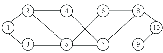
Figure 2: The communication graph

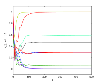
Figure 3: The trajectories of $x_{i}(t),~i=0,~1,~\cdots,~n$ under Algorithm 1.

Figure 4: The trajectories of $y_{i}(t),~i=0,~1,~\cdots,~n$ under Algorithm 1.

In this section, we use our algorithms to deal with the distributed power allocation problem of small-cell networks. Here we consider a small-cell network consisting of 10 small-cells, labeled as $\mathcal{V}=\{1,\cdots,10\}$. And each small-cell has a local small-cell base station, which can cover many users. The small-cell base stations are viewed as players. Here we use $x_{i}\in\mathbb{R}$ to denote the transmission power strategy of small cell base station $i$, the range of the transmission power strategy is given by $x_{i}\in[0,P_{i,0}]$, i.e. $\Omega_{i}=\{x_{i}|0\leq x_{i}\leq P_{i,0}\}$. We model the power allocation problem [39] as a game with bilevel structures. Each small-cell base station aims to adjust its transmission power to minimize its cost as follows. Each small-cell base station aims to adjust its transmission power to minimize its cost as follows

$$\begin{split}J_{i}(x_{i},y)=a_{i}yx_{i}-b_{i}(1+c_{i}x_{i}),~i\in\mathcal{V}\end{split}$$ (74)

where $a_{i}$, $b_{i}$ and $c_{i}$ are some constants determined by the interference from other small-cell base stations, the channel bandwidth, and the inverse of the transmission distance from small-cell base station $i$ to its users. Moreover, $y\in\mathbb{R}$ represents the price of the transmission power for the small-cell base stations, which can not be directly accessed by the small-cell and is determined by a total cost as follows.

$$\begin{split}\sum_{i=1}^{10}\left(\frac{y^{2}}{10}-a_{i}x_{i}y\right).\end{split}$$ (75)

The costs in (74) and (75) can be viewed as the costs in the outer level and the objective function in the inner level, respectively. Using the full information, we can obtain that $\sigma(x)=\frac{\sum_{i=1}^{10}a_{i}x_{i}}{2}$, which is an aggregation. Moreover, we can get that $x_{i}^{*}=P_{\Omega_{i}}\left[\frac{2b_{i}c_{i}}{a_{i}^{2}}-\frac{2\sum_{j=1}^{n}b_{j}c_{j}/a_{j}}{11a_{i}}\right]$. In the large-scale network, it is usually impossible for small-cells to use the full information of all $a_{i}$ and $x_{i}$, $i\in\mathcal{V}$. When making decisions, here we assume that each small-cell $i$ can only access the information of local objective function $\frac{y^{2}}{10}-a_{i}x_{i}y$, and can communicate with its neighbors via the connected graph shown in Fig. 2. In this formulation, the parameters are given by $a_{1}=a_{7}=a_{9}=2.5$, $a_{2}=3$, $a_{3}=a_{6}=1$, $a_{4}=2$, $a_{5}=a_{8}=a_{10}=4$, $b_{1}=b_{2}=b_{5}=3$, $b_{3}=b_{4}=b_{7}=b_{8}=b_{10}=4$, $b_{6}=5$, $b_{9}=3.5$ and $c_{i}=b_{i}$ for any $i\in\mathcal{V}$. Accordingly, the components of the Stackelberg equilibria follow that $x^{*}=[0,0,1,0.59,0,1,0.47,0.29,0.07,0.29]^{T}$ and $\sigma(x^{*})=3.4$.

Now we solve the power allocation problem by using Algorithm 1. Each small-cell $i$ maintains an estimate on its own transmission power strategy, denoted by $x_{i,t}\in\mathbb{R}$, as well as a local estimate on the price of the transmission power, denoted by $y_{i,t}\in\mathbb{R}$. We select the step-sizes as $\alpha=k=\kappa=1$ and $\eta_{t}=\frac{3}{t+4}$. And initial values of $x_{i,t}$ and $z_{i,t}$ are randomly chosen from $0$ to $1$, while initial values of $y_{i,t}$ are randomly chosen from $0$ to $5$ for all $i\in\mathcal{V}$. By running Algorithm 1, the trajectories of $x_{i,t}$ and $y_{i,t}$ are shown in Fig. 3 and Fig. 4, respectively. Letting $x_{t}=(x_{i,t},x_{-i,t})$, from Fig. 3 and Fig. 4, we see that after a period of time, $(x_{t},y_{i,t})$ approaches to $(x^{*},\sigma(x^{*}))$ for any $i\in\mathcal{V}$. Thus, the simulations are consistent with the theoretical results established in Theorem 1.

Next, we use Algorithm 2 to deal with the same problem by selecting $\delta_{1}=0.3,~\delta_{2}=0.2,~\delta_{3}=\delta_{7}=\delta_{10}=0.07,~\delta_{4}=0.06,~\delta_{5}=0.1,~\delta_{6}=\delta_{8}=0.08,~\delta_{9}=0.03$. Under Algorithm 2, the trajectories of $x_{i,t}$ and $y_{i,t}$ are shown in Fig. 5 and Fig. 6, respectively. From Fig. 5 and Fig. 6, we see that $(x_{t},y_{i,t})$ can also keep close to $(x^{*},\sigma(x^{*}))$ for any $i\in\mathcal{V}$. The simulations are consistent with the theoretical results established in Theorem 2.

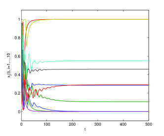
Figure 5: The trajectories of $x_{i}(t),~i=0,~1,~\cdots,~n$ under Algorithm 2.

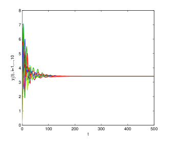
Figure 6: The trajectories of $y_{i}(t),~i=0,~1,~\cdots,~n$ under Algorithm 2.

VII Conclusions

In this paper, we have studied the problem of distributively searching the SEs of the AGs with bilevel structures, where the aggregation is determined by the minimizer of the global objective function in the inner level. To handle this problem, first, an SOGD algorithm involving the Hessain matrices associated with the objective functions in the inner level has been proposed. By implementing the algorithm, players make decisions only using the information associated with its own cost function in the outer level, a local part of the objective function in the inner part, its own action set and its own action, as well the actions of its neighbors. The result shows that if the graph is connected, then the actions of players and the estimate on the aggregation asymptotically converge to the SE. Furthermore, for the case where the Hessain matrices associated with the objective functions in the inner level are not available, we have proposed an FOGD algorithm, where a distributed two-point estimate strategy is developed to estimate the gradients of cost functions in the outer level. The result shows that the convergence errors of players’ actions and the estimate on the aggregation to the SE are linear with respect to the estimate parameters.

In our future work, some other issues on the AGs with bilevel structures will be considered, such as the case with network induced time delays, packet loss and communication bandwidth constraints, which will bring new challenges in searching the SEs in distributed manners.

Kaihong Lu received the Ph.D. degree in control theory and control engineering from Xidian University, Xi’an, China, in 2019. He is currently a Professor with the School of Electrical and Automation Engineering, Shandong University of Science and Technology, Qingdao, China. His current research interests include distributed optimization, game theory, and networked systems. Email: khong_lu@163.com

Huanshui Zhang received the B.S. degree in mathematics from Qufu Normal University, Shandong, China, in 1986, the M.Sc. degree in control theory from Heilongjiang University, Harbin, China, in 1991, and the Ph.D. degree in control theory from Northeastern University, Shenyang, China, in 1997. He was a Postdoctoral Fellow at Nanyang Technological University, Singapore, from 1998 to 2001 and Research Fellow at Hong Kong Polytechnic University, Hong Kong, China, from 2001 to 2003. He currently holds a Professorship at Shandong University of Science and Technology, Qingdao, China. He was a Professor with the Harbin Institute of Technology, Shenzhen, China, from 2003 to 2006 and a Professor with Shandong university, Jinan, China, from 2006 to 2019. His interests include optimal estimation and control, time-delay systems, stochastic systems, signal processing and wireless sensor networked systems. Email: hszhang@sdu.edu.cn

Long Wang received the bachelor’s degree in automatic control from Tsinghua University in 1986, and Ph.D. degree in Dynamics and Control from Peking University in 1992. During 1993-1997, He held postdoctoral research positions at the University of Toronto, Canada (with Professor Bruce A. Francis) and the German Aerospace Center, Munich, Germany (with Professor Juergen E. Ackermann). He is currently the Cheung-Kong Chair Professor of Dynamics and Control, and the Director of Center for Systems and Control of Peking University. His research interests include complex networked systems, evolutionary game dynamics, artificial intelligence, and bio-mimetic robotics. Prof. Wang was the recipient of the National Science Prize (in 1999 and 2017), Guan Zhaozhi Control Theory Award, Zhang Siying Award in Decision and Control, and the Best Paper Awards for journal publications in Control Theory and Applications, Science China Information Sciences, etc. Email: longwang@pku.edu.cn

References

- [1] M. K. Jensen. Aggregative games. Handbook of Game Theory and Industrial Organization, volume I, pp. 66-92, 2018.
- [2] T. Alpcan, T. Basar. A game-theoretic framework for congestion control in general topology networks. Proceedings of the 41st IEEE Conference on Decision and Control, vol. 2: pp. 1218-1224, 2002.
- [3] H. Wu, M. Shahidehpour, A. Alabdulwahab, A. Abusorrah. A game theoretic approach to risk-based optimal bidding strategies for electric vehicle aggregators in electricity markets with variable wind energy resources. IEEE Transactions on Sustainable Energy, vol. 7, no. 1, pp. 374-385, 2015.
- [4] G. I. Algazin, D. G. Algazina. Aggregate estimates of reflexive collective behavior dynamics in a Cournot oligopoly model. Automation and Remote Control, vol. 85, no. 9, pp. 923-933, 2024.
- [5] Y. You, Q. Xu, C. Fischione. Hierarchical online game-theoretic framework for real-time energy trading in smart grid. IEEE Transactions on Smart Grid, vol. 15, no. 2, pp. 1634-1645, 2024.
- [6] F. Salehisadaghiani, L. Pavel. Distributed Nash equilibrium seeking: A gossip-based algorithm. Automatica, vol. 72, pp. 209-216, 2016.
- [7] M. Ye, G. Hu. Game design and analysis for price-based demand response: An aggregate game approach. IEEE transactions on cybernetics, vol. 47, no. 3, pp.720-730, 2016.
- [8] K. Lu, G. Jing, L. Wang. Distributed algorithms for searching generalized Nash equilibrium of noncooperative games. IEEE Transactions on Cybernetics, vol. 49, no. 6, pp. 2362-2371, 2019.
- [9] F. Parise, S. Grammatico, B. Gentile, J. Lygeros. Distributed convergence to Nash equilibria in network and average aggregative games. Automatica, vol. 117, pp. 108959, 2020.
- [10] D. Paccagnan, B. Gentile, F. Parise, M. Kamgarpour, J. Lygeros. Nash and Wardrop equilibria in aggregative games with coupling constraints. IEEE Transactions on Automatic Control, vol. 64, no. 4, pp. 1373-1388, 2019.
- [11] Y. Zhu, W. Yu, G. Wen, G. Chen. Distributed Nash equilibrium seeking in an aggregative game on a directed graph. IEEE Transactions on Automatic Control, vol. 66, no. 6, pp. 2746-2753, 2021.
- [12] J. Lei, U. V. Shanbhag, J. Chen. Distributed computation of Nash equilibria for monotone aggregative games via iterative regularization. IEEE Conference on Decision and Control (CDC), pp. 2285-2290, 2020.
- [13] M. Ye, G. Hu, L. Xie, S. Xu. Differentially private distributed Nash equilibrium seeking for aggregative games. IEEE Transactions on Automatic Control, vol. 67, no. 5, pp. 2451-2458, 2022.
- [14] Y. Wang, A. Nedić. Differentially private distributed algorithms for aggregative games with guaranteed convergence. IEEE Transactions on Automatic Control, vol. 69, no. 8, pp. 5168-5183, 2024.
- [15] T. Wang, P. Yi, J. Chen, Distributed mirror descent method with operator extrapolation for stochastic aggregative games, Automatica, vol. 159, pp. 111356, 2024.
- [16] G. Belgioioso, A. Nedić, S. Grammatico. Distributed generalized Nash equilibrium seeking in aggregative games on time-varying networks. IEEE Transactions on Automatic Control, vol. 66, no. 5, pp. 2061-2075, 2021.
- [17] G. Carnevale, F. Fabiani, F. Fele, K. Margellos, G. Notarstefano. Tracking-dased distributed equilibrium seeking for aggregative games. IEEE Transactions on Automatic Control, vol. 69, no. 9, pp. 6026-6041, 2024.
- [18] S. Liang, P. Yi, Y. Hong. Distributed Nash equilibrium seeking for aggregative games with coupled constraints. Automatica, vol. 85, pp. 179-185, 2017.
- [19] M. Maljkovic, G. Nilsson, N. Geroliminis. On finding the leader’s strategy in quadratic aggregative stackelberg pricing games. European Control Conference (ECC), IEEE, pp. 1-6, 2023.
- [20] R. Li, G. Chen, D. Gan, H. Gu, J. Lü. Stackelberg and Nash equilibrium computation in non-convex leader-follower network aggregative games. IEEE Transactions on Circuits and Systems I: Regular Papers, vol. 71, no. 2, pp. 898-909, 2024.
- [21] F. Fabiani, M. A. Tajeddini, H. Kebriaei, S. Grammatico. Local Stackelberg equilibrium seeking in generalized aggregative games. IEEE Transactions on Automatic Control, vol. 67, no. 2, pp. 965-970, 2022.
- [22] M. Shokri, H. Kebriaei. Leader-follower network aggregative game with stochastic agents’ communication and activeness. IEEE Transactions on Automatic Control, vol. 65, no. 12, pp. 5496-5502, 2021.
- [23] F. Facchinei, J. S. Pang, Finite-dimensional variational inequalities and complementarity problems. Springer Science & Business Media, 2007.
- [24] K. Lu, G. Li, L. Wang. Online distributed algorithms for seeking generalized Nash equilibria in dynamic environments. IEEE Transactions on Automatic Control, vol. 66, no. 5, pp. 2289-2296, 2021.
- [25] K. Lu. Online distributed algorithms for online noncooperative games with stochastic cost functions: High probability bound of regrets. IEEE Transactions on Automatic Control, doi: 10.1109/TAC.2024.3419018, 2024.
- [26] D. Feijer, F. Paganini. Stability of primal-dual gradient dynamics and applications to network optimization. Automatica, vol. 46, no. 12, pp. 1974-1981, 2010.
- [27] Q. Ling, W. Shi, G. Wu, A. Ribeiro. DLM: Decentralized linearized alternating direction method of multipliers. IEEE Transactions on Signal Processing, vol. 63, pp. 4051-4064, 2015.
- [28] E. Y. Hamedani, N. S. Aybat. A primal-dual algorithm with line search for general convex-concave saddle point problems. SIAM Journal on Optimization, vol. 31, no. 2, pp. 1299-1329, 2021.
- [29] R. Olfati-Saber, J. A. Fax, R. M. Murray. Consensus and cooperation in networked multi-agent systems. Proceedings of the IEEE, vol. 95, no. 1, pp. 215-233, 2007.
- [30] W. Ren, R. W. Beard. Consensus seeking in multiagent systems under dynamically changing interaction topologies. IEEE Transactions on automatic control, vol. 50, no. 5, pp. 655-661, 2005.
- [31] A. Amirkhani, A. H. Barshooi. Consensus in multi-agent systems: a review. Artificial Intelligence Review, vol. 55, no. 5, pp. 3897-3935, 2022.
- [32] J. C. Duchi, A. Agarwal, M. J. Wainwright. Dual averaging for distributed optimization: Convergence analysis and network scaling. IEEE Transactions on Automatic control, vol. 57, no. 3, pp. 592-606, 2012.
- [33] Nedić A, Olshevsky A. Distributed optimization over time-varying directed graphs. IEEE Transactions on Automatic Control, vol. 60, no. 3, pp. 601-615, 2015.
- [34] S. Pu, A. Nedić. Distributed stochastic gradient tracking methods. Mathematical Programming, vol. 187, no. 1, pp. 409-457, 2021.
- [35] G. Qu, N. Li. Harnessing smoothness to accelerate distributed optimization. IEEE Transactions on Control of Network Systems, vol. 5, no. 3, pp. 1245-1260, 2018.
- [36] H. Zhang, H. Wang, Y. Xu, Z. Guo. Optimization methods rooted in optimal control. Science China: Information sciences, vol.67, pp. 222208, 2024.
- [37] K. Lu, H. Wang, H. Zhang, L. Wang. Convergence in high probability of distributed stochastic gradient descent algorithms. IEEE Transactions on Automatic Control, vol. 69, no. 4, pp. 2189-2204, 2024.
- [38] Y. F. Yang, D. H. Li, L. Qi. A feasible sequential linear equation method for inequality constrained optimization. SIAM Journal on Optimization, vol. 13, no. 4, pp. 1222-1244, 2003.
- [39] I. Hwang, B. Song, S. S. Soliman. A holistic view on hyper-dense heterogeneous and small cell networks. IEEE Communications Magazine, vol. 51, no. 6, pp. 20-27, 2013.