QuLTSF: Long-Term Time Series Forecasting
with Quantum Machine Learning

Abstract

Long-term time series forecasting (LTSF) involves predicting a large number of future values of a time series based on the past values and is an essential task in a wide range of domains including weather forecasting, stock market analysis, disease outbreak prediction. Over the decades LTSF algorithms have transitioned from statistical models to deep learning models like transformer models. Despite the complex architecture of transformer based LTSF models ‘Are Transformers Effective for Time Series Forecasting? (Zeng et al., 2023)’ showed that simple linear models can outperform the state-of-the-art transformer based LTSF models. Recently, quantum machine learning (QML) is evolving as a domain to enhance the capabilities of classical machine learning models. In this paper we initiate the application of QML to LTSF problems by proposing QuLTSF, a simple hybrid QML model for multivariate LTSF. Through extensive experiments on a widely used weather dataset we show the advantages of QuLTSF over the state-of-the-art classical linear models, in terms of reduced mean squared error and mean absolute error.

1 INTRODUCTION

Time series forecasting (TSF) is the process of predicting future values of a variable using its historical data. TSF is an import problem in many fields like weather forecasting, finance, power management etc. There are broadly two approaches to handle TSF problems: statistical models and deep learning models. Statistical models, like ARIMA, are the traditional work horse for TSF since the $1970$’s [Hyndman, 2018, Hamilton, 2020]. Deep learning models, like recurrent neural networks (RNN’s), often outperform statistical models in large-scale datasets [Lim and Zohren, 2021].

Increasing the prediction horizon strain’s the models predictive capacity. The prediction length of more than $48$ future points is generally considered as long-term time series forecasting (LTSF) [Zhou et al., 2021]. Transformers and attention mechanism proposed in [Vaswani, 2017] gained a lot of attraction to model sequence data like language, speech etc. There is a surge in the application of transformers to LTSF leading to several time series transformer models [Zhou et al., 2021, Wu et al., 2021, Zhou et al., 2022, Liu et al., 2022, Wen et al., 2023]. Despite the complicated design of transformer based models for LTSF problems, [Zeng et al., 2023] showed that a simple autoregressive model with a linear fully connected layer can outperform the state-of-the-art transformer models.

Quantum machine learning (QML) is an emerging field that combines quantum computing and machine learning to enhance tasks like classification, regression, generative modeling using the currently available noisy intermediate-scale quantum (NISQ) computers [Preskill, 2018, Schuld and Petruccione, 2021, Simeone, 2022]. Hybrid models containing classical neural networks and variational quantum circuits (VQC’s) are increasingly becoming popular for various machine learning tasks, thanks to rapidly evolving software tools [Bergholm et al., 2018]. The existing QML models for TSF focus on RNN’s [Emmanoulopoulos and Dimoska, 2022, Ceschini et al., 2022]. In time series analysis, recurrent quantum circuits have demonstrated provable computational and memory advantage during inference, however learning such models remains challenging at scale [Binder et al., 2018]. To the best of our knowledge there is no QML model for LTSF problems.

In this paper we initiate the application of QML to LTSF by proposing QuLTSF a simple hybrid QML model. QuLTSF is a combination of classical linear neural networks and VQC’s. Through extensive experiments, on the widely used weather dataset, we show that the QuLTSF model outperforms the state-of-the-art linear models proposed in [Zeng et al., 2023].

Organization of the paper: Section $2$ provides background information on quantum computing and quantum machine learning. Section $3$ discusses the problem formulation and related work. In Section $4$ we introduce our QuLTSF model. Experimental details and results are given in Section $5$ and Section $6$ concludes the paper.

2 BACKGROUND

2.1 Quantum Computing

The fundamental unit of quantum information and computing is the qubit. In contrast to a classical bit, which exist in either $0$ or $1$ state, the state of a qubit can be $0$ or $1$ or a superposition of both. In the Dirac’s ket notation the state of a qubit is given as a two-dimensional amplitude vector

$$|\psi\rangle=\begin{bmatrix}\alpha_{0}\\ \alpha_{1}\end{bmatrix}=\alpha_{0}|0\rangle+\alpha_{1}|1\rangle,$$

where $\alpha_{0}$ and $\alpha_{1}$ are complex numbers satisfying the unitary norm condition, i.e., $|\alpha_{0}|^{2}+|\alpha_{1}|^{2}=1$. The state of a qubit is only accessible through measurements. A measurement in the computational basis collapses the state $|\psi\rangle$ to a classical bit $x\in\{0,1\}$ with probability $|\alpha_{x}|^{2}$. A qubit can be transformed from one state to another via reversible unitary operations also known as quantum gates [Nielsen and Chuang, 2010].

Shor’s algorithm [Shor, 1994] and Grover’s algorithm [Grover, 1996] revolutionized quantum algorithms research by providing theoretical quantum speedups compared to classical algorithms. The implementation of these algorithms require larger number of qubits with good error correction [Lidar and Brun, 2013]. However, the current available quantum devices are far from this and often referred to as the noisy intermediate-scale quantum (NISQ) devices [Preskill, 2018]. Quantum machine learning (QML) is an emerging field to make best use of NISQ devices [Schuld and Petruccione, 2021, Simeone, 2022].

2.2 Quantum Machine Learning

The most common QML paradigm refers to a two step methodology consisting of a variational quantum circuit (VQC) or ansatz and a classical optimizer, where VQC is composed of parametrized quantum gates and fixed entangling gates. The classical data is first encoded into a quantum state, using a suitable data embedding procedure. Then, the VQC applies a parametrized unitary operation which can be controlled by altering its parameters. The output of the quantum circuit is given by measuring the qubits. The parameters of the VQC are optimized using classical optimization tools to minimize a predefined loss function. Often VQC’s are paired with classical neural networks, creating hybrid QML models. Several packages, for instance [Bergholm et al., 2018], provide software tools to efficiently compute gradients for these hybrid QML models.

3 PRELIMINARIES

3.1 Problem Formulation

Consider a multivariate time series dataset with $M$ variates. Let $L$ be the size of the look back window or sequence length and $T$ be the size of the forecast window or prediction length. Given data at $L$ time stamps $\mathbf{x}_{1:L}=\{\mathbf{x}_{1},\cdots,\mathbf{x}_{L}\}\in\mathbb{R}^{L\times M}$, we would like to predict the data at future $T$ time stamps $\mathbf{\hat{x}}_{L+1:L+T}=\{\mathbf{\hat{x}}_{L+1},\cdots,\mathbf{\hat{x}}_{L+T}\}\in\mathbb{R}^{T\times M}$ using a QML model. Predicting more than $48$ future time steps is typically considered as Long-term time series forecasting (LTSF) [Zhou et al., 2021]. We consider the channel-independence condition where each of the univariate time series data at $L$ time stamps $\mathbf{x}^{m}_{1:L}=\{x^{m}_{1},\cdots,x^{m}_{L}\}\in\mathbb{R}^{L\times 1}$ is fed separately into the model to predict the data at future $T$ time stamps $\mathbf{\hat{x}}^{m}_{L+1:L+T}=\{\hat{x}^{m}_{L+1},\cdots,\hat{x}^{m}_{L+T}\}\in\mathbb{R}^{T\times 1}$, where $m\in\{1,\cdots,M\}$. To measure discrepancy between the ground truth and prediction, we use Mean Squared Error (MSE) loss function defined as

$$\text{MSE}=\mathbb{E}_{\mathbf{x}}\Biggr{[}\frac{1}{M}\sum_{m=1}^{M}\|\mathbf{x}^{m}_{L+1:L+T}-\mathbf{\hat{x}}^{m}_{L+1:L+T}\|_{2}^{2}\Biggr{]}.$$ (1)

3.2 Related Work

LTSF is an extensive area of research. In this section, we provide a concise overview of works most relevant to our problem formulation. Since the introduction of transformers [Vaswani, 2017], there has been an increase in transformer based models for LTSF [Wu et al., 2021, Zhou et al., 2021, Liu et al., 2022, Zhou et al., 2022, Li et al., 2019]. [Wen et al., 2023] provided a comprehensive survey on transformer based LTSF models. Despite the sophisticated architecture of transformer based LTSF models, [Zeng et al., 2023] showed that simple linear models can achieve superior performance compared to the state-of-the-art transformer based LTSF models.

[Zeng et al., 2023] proposed three models: Linear, NLinear and DLinear. Linear model is just a one layer linear neural network. In NLinear, the last value of the input is subtracted before being passed through the linear layer and the subtracted part is added back to the output. DLinear first decomposes the time series into trend, by a moving average kernel, and seasonal components which is a famous method in time series forecasting [Hamilton, 2020] and is extensively used in the literature [Wu et al., 2021, Zhou et al., 2022, Zeng et al., 2023]. Two similar but distinct linear models are trained for trend and seasonal components. Adding the outputs of these two models gives the final prediction. We adapt the simple Linear model to propose our QML model in the next section.

4 QuLTSF

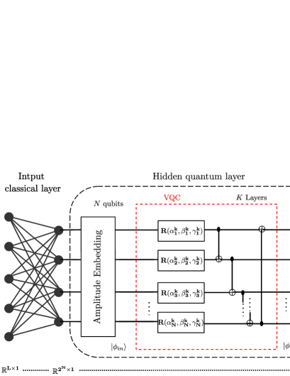
Figure 1: QuLTSF model architecture.

In this section, we propose QuLTSF a hybrid QML model for LTSF and is illustrated in Fig. 1. It is a hybrid model consisting of input classical layer, hidden quantum layer and an output classical layer. The input classical layer maps the $L$ input features in to a $2^{N}$ length vector. Specifically, the input sequence $\mathbf{x}^{m}_{1:L}\in\mathbb{R}^{L\times 1}$ is given to the input classical layer with trainable weights $\mathbf{W}_{in}\in\mathbf{R}^{2^{N}\times L}$ and bias $\mathbf{b}_{in}\in\mathbf{R}^{2^{N}\times 1}$, and it outputs a $2^{N}$ length vector

$$\mathbf{y}_{1}=\mathbf{W}_{in}\mathbf{x}^{m}_{1:L}+b_{in}.$$ (2)

The output of the input classical layer, $y_{1}\in\mathbf{R}^{2^{N}\times 1}$, is given as input to the hidden quantum layer which consists of $N$ qubits. We use amplitude embedding [Schuld and Petruccione, 2021] to encode $2^{N}$ real numbers in $y_{1}$ to a quantum state $|\phi_{in}\rangle$. We use hardware efficient ansatz [Simeone, 2022] as a VQC, and is composed of $K$ layers each containing a trainable parametrized single qubit gate on each qubit and a fixed circular entangling circuit with CNOT gates as shown in Fig. 1. Every single qubit gate has $3$ parameters and the total number of parameters in $K$ layers is $3NK$. The output of VQC is given as

$$|\phi_{out}\rangle=(\text{VQC})|\phi_{in}\rangle.$$ (3)

We consider the expectation value of Pauli-$Z$ observable for each qubit, which serves as the output of hidden quantum layer and is denoted as $y_{2}\in\mathbb{R}^{N\times 1}$. Finally, $y_{2}$ is passed through output classical layer with trainable weights $\mathbf{W}_{out}\in\mathbf{R}^{T\times N}$ and bias $\mathbf{b}_{out}\in\mathbf{R}^{T\times 1}$, which maps $N$ length quantum hidden layer output to predicted $T$ length vector

$$\mathbf{\hat{x}}^{m}_{L+1:L+T}=\mathbf{W}_{out}\mathbf{y}_{2}+b_{out}.$$ (4)

The parameters of the hidden quantum layer and two classical layers can be jointly trained, similar to classical machine learning, using software packages like PennyLane [Bergholm et al., 2018].

5 EXPERIMENTS

In this section, we validate the superiority of the proposed QuLTSF model through extensive experiments. The code for experiments is publicly available on GitHub. All experiments are conducted on SMU’s Crimson GPU cluster.

Table 1: Multivariate long-term time series forecasting (LTSF) results in terms of MSE and MAE between the proposed QuLTSF model and the state-of-the-art on the widely used weather dataset. Sequence length $L=336$ and prediction length $T\in\{96,192,336,720\}$. The best results are in bold and the second best results are underlined.

Methods QuLTSF* Linear NLinear DLinear FEDformer Autoformer Informer Metric MSE MAE MSE MAE MSE MAE MSE MAE MSE MAE MSE MAE MSE MAE $96$ $\mathbf{0.156}$ $\mathbf{0.211}$ $\underline{0.176}$ $0.236$ $0.182$ $\underline{0.232}$ $\underline{0.176}$ $0.237$ $0.217$ $0.296$ $0.266$ $0.336$ $0.300$ $0.384$ $192$ $\mathbf{0.199}$ $\mathbf{0.253}$ $\underline{0.218}$ $0.276$ $0.225$ $\underline{0.269}$ $0.220$ $0.282$ $0.276$ $0.336$ $0.307$ $0.367$ $0.598$ $0.544$ $336$ $\mathbf{0.248}$ $\mathbf{0.296}$ $\underline{0.262}$ $0.312$ $0.271$ $\underline{0.301}$ $0.265$ $0.319$ $0.339$ $0.380$ $0.359$ $0.395$ $0.578$ $0.523$ $720$ 0.315 0.346 $0.326$ $0.365$ $0.338$ $\underline{0.348}$ $\underline{0.323}$ $0.362$ $0.403$ $0.428$ $0.419$ $0.428$ $1.059$ $0.741$

*QuLTSF is implemented by us; Other results are from [Zeng et al., 2023].

5.1 Dataset Description

We evaluate the performance of our proposed QuLTSF model on the widely used Weather dataset. It is recorded by Max-Planck Institute of Biogeochemistry and consists of $21$ meteorological and environmental features like air temperature, humidity, carbon dioxide concentration in parts per million etc. This is recorded in 2020 with granularity of 10 minutes and contains $52,696$ timestamps. $70$ percent of the available data is used for training, $20$ percent for testing and the remaining data for validation.

5.2 Baselines

We choose all three state-of-the-art linear models namely Linear, NLinear and DLinear proposed in [Zeng et al., 2023] as the main baselines. We also consider a few transformer based LTSF models FEDformer [Zhou et al., 2022], Autoformer [Wu et al., 2021], Informer [Zhou et al., 2021] as other baselines. Moreover [Wu et al., 2021, Zhou et al., 2021] showed that transformer based models outperform traditional statistical models like ARIMA [Box et al., 2015] and other deep learning based models like LSTM [Bai et al., 2018] and DeepAR[Salinas et al., 2020], thus we do not include them in our baselines.

5.3 Evaluation Metrics

Following common practice, in the state-of-the-art we use MSE (1) and Mean Absolute Error (MAE) (5) as evaluation metrics

$$\text{MAE}=\mathbb{E}_{\mathbf{x}}\Biggr{[}\frac{1}{M}\sum_{m=1}^{M}||\mathbf{x}^{m}_{L+1:L+T}-\mathbf{\hat{x}}^{m}_{L+1:L+T}||_{1}\Biggr{]}.$$ (5)

5.4 Hyperparameters

The number of qubits $N=10$ and number of VQC layers $K=3$ in the hidden quantum layer. Adam optimizer [Kingma and Ba, 2017] is used to train the model in order to minimize the MSE over the training set. Other hyperparameters are adapted from [Zeng et al., 2023]. For more hyperparameters refer to our code.

5.5 Results

For a fair comparison, we choose the fixed sequence length $L=336$ and $4$ different prediction lengths $T\in\{96,192,336,720\}$ as in [Zeng et al., 2023, Zhou et al., 2022, Wu et al., 2021, Zhou et al., 2021]. Table 1 provides comparison of MSE and MAE of QuLTSF with $6$ baselines. The best and second best results are highlighted in bold and underlined respectively. Our proposed QuLTSF outperform all the baseline models in all $4$ cases.

To further validate QuLTSF against the baseline linear models we conduct experiments with varying sequence lengths $L\in\{48,96,192,336,504,720\}$ and plot the MSE results for a fixed smaller prediction length $T=96$ in Fig. 2, and for a fixed larger prediction length $T=720$ in Fig. 3. In all cases QuLTSF outperforms all the baseline linear models.

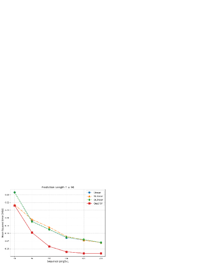
Figure 2: MSE comparison with fixed prediction length $T=96$ and varying sequence length $L\in\{48,96,192,336,504,720\}$.

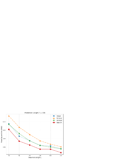
Figure 3: MSE comparison with fixed prediction length $T=720$ and varying sequence length $L\in\{48,96,192,336,504,720\}$.

5.6 Discussion and Future Work

QuLTSF uses generic hardware-efficient ansatz. Similar to classical machine learning in QML we need to choose the ansatz, if possible, based on dataset and domain expertise. Searching for optimal ansatz is a research direction by itself [Du et al., 2022]. Finding better ansatzes for QML based LTSF models for different datasets is an open problem. One potential way is to use parameterized two qubit rotation gates [You et al., 2021].

Other possible future direction is to use efficient data preprocessing, for example reverse instance normalization [Kim et al., 2021] to mitigate the distribution shift between training and testing data. This is already being used in the state-of-the-art transformer based LTSF models like PatchTST [Nie et al., 2023] and MTST [Zhang et al., 2024]. These models also show better performance than the linear models in [Zeng et al., 2023]. Interestingly, our simple QuLTSF model outperforms or comparable to these models in limited settings. For instance, for the setting $(L=336,T=720)$ MSE of PatchTST, MTST and QuLTSF are $0.320$, $\underline{0.319}$ and $\mathbf{0.315}$ respectively. For the setting $(L=336,T=336)$ MSE of PatchTST, MTST and QuLTSF are $0.249$, $\mathbf{0.246}$ and $\underline{0.248}$ respectively (see Table $2$ in [Zhang et al., 2024] for PatchTST and MTST; and Table 1 for QuLTSF). Thus, QML models with efficient data preprocessing may lead to improved results.

6 CONCLUSIONS

We proposed QuLTSF, a simple hybrid QML model for LTSF problems. QuLTSF combines the power of VQC’s with classical linear neural networks to form an efficient LTSF model. While the simple linear models outperform the complex transformer based LTSF models, the introduction of hidden quantum layer further improved the performance. This opens up a new direction of applying hybrid QML models for future LTSF research.

REFERENCES

- Bai et al., 2018 Bai, S., Kolter, J. Z., and Koltun, V. (2018). An empirical evaluation of generic convolutional and recurrent networks for sequence modeling. arXiv preprint arXiv:1803.01271.
- Bergholm et al., 2018 Bergholm, V., Izaac, J., Schuld, M., Gogolin, C., Ahmed, S., Ajith, V., Alam, M. S., Alonso-Linaje, G., AkashNarayanan, B., Asadi, A., et al. (2018). Pennylane: Automatic differentiation of hybrid quantum-classical computations. arXiv preprint arXiv:1811.04968.
- Binder et al., 2018 Binder, F. C., Thompson, J., and Gu, M. (2018). Practical unitary simulator for non-markovian complex processes. Physical review letters, 120(24):240502.
- Box et al., 2015 Box, G. E., Jenkins, G. M., Reinsel, G. C., and Ljung, G. M. (2015). Time series analysis: forecasting and control. John Wiley & Sons.
- Ceschini et al., 2022 Ceschini, A., Rosato, A., and Panella, M. (2022). Hybrid quantum-classical recurrent neural networks for time series prediction. In 2022 International Joint Conference on Neural Networks (IJCNN), pages 1–8.
- Du et al., 2022 Du, Y., Huang, T., You, S., Hsieh, M.-H., and Tao, D. (2022). Quantum circuit architecture search for variational quantum algorithms. npj Quantum Information, 8(1):62.
- Emmanoulopoulos and Dimoska, 2022 Emmanoulopoulos, D. and Dimoska, S. (2022). Quantum machine learning in finance: Time series forecasting. arXiv preprint arXiv:2202.00599.
- Grover, 1996 Grover, L. K. (1996). A fast quantum mechanical algorithm for database search. In Proceedings of the twenty-eighth annual ACM symposium on Theory of computing, pages 212–219.
- Hamilton, 2020 Hamilton, J. D. (2020). Time series analysis. Princeton university press.
- Hyndman, 2018 Hyndman, R. (2018). Forecasting: principles and practice. OTexts.
- Kim et al., 2021 Kim, T., Kim, J., Tae, Y., Park, C., Choi, J.-H., and Choo, J. (2021). Reversible instance normalization for accurate time-series forecasting against distribution shift. In International Conference on Learning Representations.
- Kingma and Ba, 2017 Kingma, D. P. and Ba, J. (2017). Adam: A method for stochastic optimization.
- Li et al., 2019 Li, S., Jin, X., Xuan, Y., Zhou, X., Chen, W., Wang, Y.-X., and Yan, X. (2019). Enhancing the locality and breaking the memory bottleneck of transformer on time series forecasting. Advances in neural information processing systems, 32.
- Lidar and Brun, 2013 Lidar, D. A. and Brun, T. A. (2013). Quantum error correction. Cambridge university press.
- Lim and Zohren, 2021 Lim, B. and Zohren, S. (2021). Time-series forecasting with deep learning: a survey. Philosophical Transactions of the Royal Society A, 379(2194):20200209.
- Liu et al., 2022 Liu, S., Yu, H., Liao, C., Li, J., Lin, W., Liu, A. X., and Dustdar, S. (2022). Pyraformer: Low-complexity pyramidal attention for long-range time series modeling and forecasting. In International Conference on Learning Representations.
- Nie et al., 2023 Nie, Y., Nguyen, N. H., Sinthong, P., and Kalagnanam, J. (2023). A time series is worth 64 words: Long-term forecasting with transformers. In The Eleventh International Conference on Learning Representations.
- Nielsen and Chuang, 2010 Nielsen, M. A. and Chuang, I. L. (2010). Quantum computation and quantum information. Cambridge university press.
- Preskill, 2018 Preskill, J. (2018). Quantum computing in the nisq era and beyond. Quantum, 2:79.
- Salinas et al., 2020 Salinas, D., Flunkert, V., Gasthaus, J., and Januschowski, T. (2020). Deepar: Probabilistic forecasting with autoregressive recurrent networks. International journal of forecasting, 36(3):1181–1191.
- Schuld and Petruccione, 2021 Schuld, M. and Petruccione, F. (2021). Machine learning with quantum computers, volume 676. Springer.
- Shor, 1994 Shor, P. (1994). Algorithms for quantum computation: discrete logarithms and factoring. In Proceedings 35th Annual Symposium on Foundations of Computer Science, pages 124–134.
- Simeone, 2022 Simeone, O. (2022). An introduction to quantum machine learning for engineers. Found. Trends Signal Process., 16(1–2):1–223.
- Vaswani, 2017 Vaswani, A. (2017). Attention is all you need. Advances in Neural Information Processing Systems. Neural information processing systems foundation, page 5999.
- Wen et al., 2023 Wen, Q., Zhou, T., Zhang, C., Chen, W., Ma, Z., Yan, J., and Sun, L. (2023). Transformers in time series: a survey. In Proceedings of the Thirty-Second International Joint Conference on Artificial Intelligence, pages 6778–6786.
- Wu et al., 2021 Wu, H., Xu, J., Wang, J., and Long, M. (2021). Autoformer: Decomposition transformers with auto-correlation for long-term series forecasting. Advances in neural information processing systems, 34:22419–22430.
- You et al., 2021 You, J.-B., Koh, D. E., Kong, J. F., Ding, W.-J., Png, C. E., and Wu, L. (2021). Exploring variational quantum eigensolver ansatzes for the long-range xy model. arXiv preprint arXiv:2109.00288.
- Zeng et al., 2023 Zeng, A., Chen, M., Zhang, L., and Xu, Q. (2023). Are transformers effective for time series forecasting? In Proceedings of the AAAI conference on artificial intelligence, volume 37, pages 11121–11128.
- Zhang et al., 2024 Zhang, Y., Ma, L., Pal, S., Zhang, Y., and Coates, M. (2024). Multi-resolution time-series transformer for long-term forecasting. In International Conference on Artificial Intelligence and Statistics, pages 4222–4230. PMLR.
- Zhou et al., 2021 Zhou, H., Zhang, S., Peng, J., Zhang, S., Li, J., Xiong, H., and Zhang, W. (2021). Informer: Beyond efficient transformer for long sequence time-series forecasting. In Proceedings of the AAAI conference on artificial intelligence, volume 35, pages 11106–11115.
- Zhou et al., 2022 Zhou, T., Ma, Z., Wen, Q., Wang, X., Sun, L., and Jin, R. (2022). Fedformer: Frequency enhanced decomposed transformer for long-term series forecasting. In International conference on machine learning, pages 27268–27286. PMLR.