Three-dimensional real space renormalization group with well-controlled approximations

Abstract

We make Kadanoff’s block idea into a reliable three-dimensional (3D) real space renormalization group (RG) method. Kadanoff’s idea, expressed in spin representation, offers a qualitative intuition for clarifying scaling behavior in criticality, but has difficulty as a quantitative tool due to uncontrolled approximations. A tensor-network reformulation equips the block idea with a measure of RG errors. In 3D, we propose an entanglement filtering scheme to enhance such a block-tensor map, with the lattice reflection symmetry imposed. When the proposed RG is applied to the cubic-lattice Ising model, the RG errors are reduced to about 2% by retaining more couplings. The estimated scaling dimensions of the two relevant fields have errors 0.4% and 0.1% in the best case, compared with the accepted values. The proposed RG is promising as a systematically-improvable real space RG method in 3D. The unique feature of our method is its ability to numerically obtain a 3D critical fixed point in a high-dimensional tensor space. A fixed-point tensor contains much more information than a handful of observables estimated in conventional techniques for analyzing critical systems.

Introduction— The renormalization group (RG) idea offers both a theoretical framework for understanding the universality in critical phenomena [1] and a practical approach for calculating the critical exponents [2, 3] that quantify a universality class. The key operation of the RG idea is a coarse-graining process to generate a series of descriptions of a system in increasingly larger length scales, represented by a flow in the coupling-constant space known as an RG flow. Phase transitions belonging to the same universality class correspond to the same critical fixed point of these RG flows. The critical exponents can be calculated from scaling dimensions $\{x_{i}\}$, which are defined using the eigenvalues $\{\lambda_{i}\}$ of the linearized RG flow around the critical fixed point,

$$b^{d-x_{i}}=\lambda_{i},$$ (1)

where $d$ is the spatial dimensionality of the thermodynamic system and $b$ is the rescaling factor of the coarse-graining.

Kadanoff’s block-spin idea [4] is the prototype of the RG in real space: a block of spins are replaced with one coarser spin, provided that the partition function is preserved. For spatial dimensionality $D\geq 2$, if the partition function is preserved exactly, a single step of this RG map entails all possible interaction terms among spins with all ranges [5]. When designing a practical numerical RG method, we have to truncate the coupling-constant space down to finite dimensions.

Using a drastic approximation, Migdal [6] and Kadanoff [7] proposed a bond-moving scheme that decouples the interactions in different spatial directions. This Migdal-Kadanoff (MK) approach maintains the nearest-neighbor interaction form and is applicable in any spatial dimensionality. However, MK approach only works well when the transition temperature is close or equal to zero, or equivalently the spatial dimensionality is near the lower critical dimension. This is, for example, not true for the Ising model in 2D and 3D, and the estimate of thermal exponents $\nu$ has error almost $50\%$ for 3D and $25\%$ for 2D, which are very crude approximations. Martinelli and Parisi [8] designed a systematical improvement of MK approach. For the 3D Ising model, the first-order corrections move MK estimates of $\nu$ closer to the accepted value. However, no higher-order corrections have been computed.

Above all, there is no a priori quantitative metric to assess the approximations made in these spin-based RG transformations; the justification usually comes from an a posteriori comparison with the accepted estimates of various critical exponents. Therefore, apart from an intuitive feeling that they could work, one might feel uneasy to trust them as precise numerical methods [9].

In this paper, we propose an RG transformation in real space for any three-dimensional (3D) classical statistical system on a lattice . Our method is based on a tensor-network reformulation of the real space RG [11, 12], which has a natural metric for quantifying the RG approximation errors. Our main contribution is designing a workable 3D entanglement filtering scheme based on Refs. [13, 14] to enhance the usual block-tensor transformation, with the lattice reflection symmetry imposed. This is essential for obtaining a critical fixed-point tensor and taming the growth of RG errors with the RG step in 3D. The estimated scaling dimensions of the spin and the energy density fields $x_{\sigma},x_{\epsilon}$, compared with the conformal bootstrap estimates [15, 16], have relative errors $0.4\%$ and $0.1\%$ in the best case.

Block-tensor transformation— A reformulation of the real space RG in the tensor-network language equips it with a natural measure of the RG approximation error [11, 12]. This reformulation is inspired by concepts like entanglement entropy from quantum information and numerical tools for analyzing (1+1)D quantum many-body systems, such as the density-matrix renormalization group (DMRG) [17] and tensor-network ansatz [18, 19]. We refer to this modern reformulation as the tensor-network renormalization group (TNRG). In TNRG, the partition function is encoded in a local tensor capturing the Boltzmann weight, as well as how these local tenors connect with each other to form a tensor network. Kadanoff’s block idea becomes a block-tensor transformation. For example, in a square-lattice tensor network, a TNRG defines an RG transformation in the space of 4-leg tensors,

$$A\mapsto A_{c},$$ (2)

where both $A$ and $A_{c}$ are tensors with four indices. In numerical calculations, each index (or leg) has a finite dimensionality $\chi\in\mathbb{Z}$ called the bond dimension, which corresponds to the number of coupling constants retained during the RG. There are many practical block-tensor schemes [11, 20, 21, 22, 23], all of whose basic ideas dates back to the DMRG. In 2D, these methods inherit the high accuracy of the DMRG for (1+1)D quantum systems, according to the quantum-to-classical map [24, 25]; their success is assured for non-critical systems due to the saturation of entanglement entropy [11, 26]. Similar to the DMRG, what measures the RG approximation error in the TNRG is how fast the eigenvalues of some density matrix decay. The relative error of the estimated free energy of the 2D Ising model can easily go down to $\sim 10^{-9}$ using a personal computer [27].

Entanglement filtering in 3D— The justification for the success of the 2D block-tensor schemes no longer works in 3D due to the growth of entanglement entropy [26]. This is not because of the much higher computational complexity in 3D, but because of a qualitative difference between 2D and 3D in their entanglement structure. In our numerical experiment using the go-to block-tensor map in 3D, the higher-order tensor renormalization group (HOTRG) [20], we observe that for bond dimension $\chi\leq 22$, the RG errors grow rapidly to more than $10\%$ just after one RG step, and then keep growing to more than $30\%$ near the critical fixed point of the cubic-lattice Ising model. Moreover, the RG errors near the critical region grow slowly (not decrease!) with the bond dimension, which makes unreliable the block-tensor map in 3D.

A way out for this growth of entanglement entropy is to enhance the simple block-tensor transformation with an entanglement filtering (EF) process [28, 29, 30]. If designed carefully, an EF scheme can significantly reduce the entanglement entropy in the coarse-grained description and hence reduce the RG errors of the block-tensor transformation [29, 30]. There are many EF schemes[29, 28, 30, 31, 32, 13, 14, 33, 34] in 2D but a workable 3D scheme is still missing.

Two ideas are essential for a 3D EF scheme: graph independence and imposing the necessary symmetries of the microscopic model. If an EF process does not alter the graph formed by the tensor network, it is called graph independent [13]. Graph independence makes an entanglement filtering a standalone procedure, which can be incorporated into any block-tensor schemes. This versatility is essential for designing a 3D EF-enhanced TNRG.

To obtain a critical fixed-point tensor, it is crucial to impose necessary symmetries of the microscopic model in the TNRG. Without symmetries being imposed, even if we start from symmetric initial tensors, numerical errors associated with machine precision, or even worse, with the artifacts of a chosen scheme, introduce all possible perturbations away from the critical model located on the critical surface. Since a few RG steps are needed to drive this critical model to the corresponding critical fixed point, those perturbations along the RG relevant directions inevitably get amplified. This entails difficulty in obtaining a critical fixed-point tensor. People have developed mature framework for imposing global on-site symmetry [35], like the spin-flip $\mathbb{Z}_{2}$ symmetry of the Ising model [36]. For the 2D Ising model, it is enough to impose the spin-flip $\mathbb{Z}_{2}$ symmetry because the only RG relevant direction in the spin-flip even sector is the energy density field $\epsilon$, which corresponds to the fine-tuning of the temperature to its critical value $T_{c}$. For the 3D Ising model, however, there are more RG relevant directions. Besides the energy density field $\epsilon$, whose scaling dimension is about 1.41, its three first descendants, $\partial_{x}\epsilon,\partial_{y}\epsilon,\partial_{z}\epsilon$, have scaling dimension about 2.41, smaller than the spatial dimension 3 [37].

In our numerical experiment, adding a naive 3D generalization of the scheme in Ref. [13] to the HOTRG makes it harder to obtain a critical fixed-point tensor. We conjecture that it is because this naive generalization breaks the lattice reflection and rotation symmetry explicitly; this numerical artifact could introduce perturbations in directions of $\partial_{x}\epsilon,\partial_{y}\epsilon,\partial_{z}\epsilon$. To eliminate these directions in the RG map, we develop techniques for imposing lattice reflection symmetry in TNRG. The unique feature of our proposed EF scheme is that it is both graph independent and with the lattice reflection symmetry imposed. The gist of the proposed EF is captured in the following approximation in 2D,

$$\includegraphics[width=151.76633pt,valign={c}]{ee2D-approx.png},$$ (3)

where the two filtering matrices $s_{x},s_{y}$ squeeze the bond dimension from $\chi$ to $\chi_{s}<\chi$, while we want the plaquette after this squeezing remains as close as the original one. The double arrow along the horizontal or the vertical axis means the two legs along that direction are transposed. For example, $\includegraphics[scale={0.02},valign={c},raise={0em}]{Aarrx.png}\stackrel{{\scriptstyle\text{def}}}{{=}}\includegraphics[scale={0.02},valign={c},raise={0em}]{Atx.png}$. The reason why this transposition trick can impose lattice-reflection symmetry will be explained in a coming paper. These filtering matrices are initialized according to the technique in Ref. [13] and further optimized using the method developed in Ref. [14], by maximizing the overlap between the filtered state $|\phi\rangle$ and the target state $|\psi\rangle$ in Eq. (3). The 3D generalization is in Eq. (5).

How to integrate an EF into a block-tensor map— A block-tensor transformation fails to simplify microscopic entanglement located near the intersection regions of groups of spins [29]. In a 2D block-tensor map, these boundary entanglement transforms like

$$\includegraphics[width=86.72267pt,valign={c}]{TN2spin.png},$$ (4a)

$$\includegraphics[width=173.44865pt,valign={c}]{2dblock-ee.png}.$$ (4b)

These two equations are intuitive in nature, whose more precise form can be understood using corner-double-line tensors [11, 28]. The correspondence in Eq. (4a) demonstrates the relationship between the 4-leg tensor and the original spins, where the blue arrows denotes the original spin degrees of freedom and the shaded dots $c$ marks the location of boundary entanglement. Under the block-tensor transformation in Eq. (4b), the entanglement among the spins in the region around the center of the block denoted by $o$ is renormalized to a single number after the spins on the inner edges are summed over. The entanglement around the center of the edge denoted by $u$ is among spins on the same edge of a larger block, and thus will be renormalized after a isometric transformation in the block-tensor map [30, 38]. The entanglement located around four corners denoted by $c$ behaves differently and fails to be eliminated under the block-tensor map. Equation (4) is the tensor-network incarnation of the entanglement-entropy area law [26].

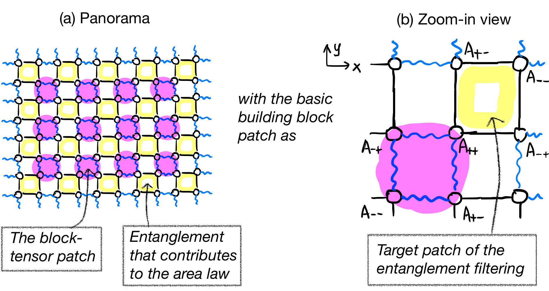
Figure 1: Location of the leftover entanglement for a 2D block-tensor transformation

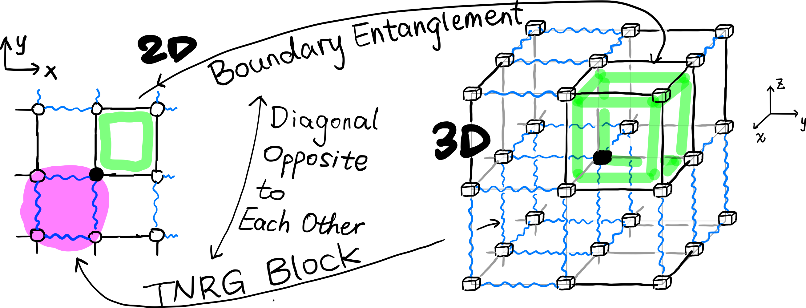
Figure 2: The general principle for integrating entanglement filtering into a block-tensor map in any spatial dimensionality, demonstrated in the 2D and the 3D.

Therefore, the EF should target patches of tensor network where the short-range entanglement fails to be eliminated under the block-tensor map (see Figure 1). Let us write down a principle of how to integrate the EF into a block-tensor map in 2D (see the 2D diagram in Figure 2), in such a way that the 3D generalization is straightforward:

Step 1: Choose an anchor point in the $2\times 2$ block tensor patch; we indicate it using a black dot at the center; put the main tensor at the anchor point.

Step 2: Draw the two legs of the main tensor that points to the positive $x$ and $y$ directions as black lines and call them “outer legs”; these two legs span the plaquette that is the target of the entanglement filtering (see Figure 1).

Step 3: Draw the two legs of the main tensor that points to the negative directions as blue wavy lines and call them “inner legs”; these two legs span the plaquette that is under the block tensor transformation (see Figure 1).

In summary, the relationship between the block-tensor patch and the EF one is that they are diagonally opposite to each other with respect to the anchor point. The generalization to 3D is straightforward (see Figure 2). Recently, an exact treatment of the 3D TNRG adopts a similar idea [39].

The proposed RG transformation— Apply the EF to the target patch shown in Figure 2 and find good choices of the filtering matrices in three directions, $s_{x},s_{y},s_{z}$, according to the approximation (the anchor point is denoted as $(+++)$):

$$\includegraphics[width=184.28981pt,valign={c}]{cubeAppro.png}.$$ (5a)

We call this a cube filtering since the target patch is a $$2\times 2\times 2$$ cube. The lattice-reflection symmetry is imposed in this step by the following transposition trick,

$$\includegraphics[width=184.28981pt,valign={c}]{cubeEnvRefl.png}.$$ (5b)

The diagrammatic notation in Eq. (5) and the strategy for finding good filtering matrices have been outlined below Eq. (3). The computational costs of finding good $s_{x},s_{y},s_{z}$ are $O(\chi^{12})$. Then, apply the filtering matrices on the three “outer legs” of the tensor at the anchor point, after which the TNRG block in Figure 2 looks like

$$\includegraphics[width=195.12767pt,valign={c}]{cubeFilter.png}.$$ (6)

Notice that the position of the anchor point $(+++)$ in Eq. (6) is different from that in Eq. (5b). If the choice of filtering matrices are good, this step should filter out boundary entanglement structures in the 3D TNRG block [13, 26].

After the cube filtering, we apply an HOTRG-like block-tensor transformation to the TNRG block. We adopt the HOTRG idea of coarse-graining one direction at a time and choose (arbitrarily) the order to be $z\rightarrow y\rightarrow x$. We demonstrate the $z$-direction collapse using the two tensors at the $(+++)$ and $(++-)$ positions in Eq. (6),

$$\includegraphics[width=173.44865pt,valign={c}]{zblock.png}.$$ (7a)

The difference between the usual HOTRG and this one is that isometric tensors are different for inner and outer legs of the tensors in the block-tensor patch. For the outer legs, the isometric tensors are $$p_{mx},p_{my} \chi_{m} p_{ix},p_{iy} \chi_{i} y (++) (+-)$$, with the output bond dimension ; for the inner legs, they are , with the output bond dimension . We use the projective truncations developed in Ref. [12] to determine these isometric tensors. For the direction, we focus on the tensors at the and in Eq. (7a),

$$\includegraphics[width=173.44865pt,valign={c}]{yblock.png}.$$ (7b)

Finally, for the $$x$$ direction, we have

$$\includegraphics[width=173.44865pt,valign={c}]{xblock.png}\,.$$ (7c)

The computational costs of our block-tensor map are $O(\chi^{12.5})$ when we use $\chi_{i}=\chi^{1.5},\chi_{ii}=\chi^{2}$ and $\chi_{s}\leq\chi_{m}\leq\chi$. The composition of the entanglement filtering map, $A\mapsto A_{s}$ in Eq. (6), with the HOTRG-like block-tensor transformation, $A_{s}\mapsto A_{c}$ in Eq. (7), gives the proposed EF-enhanced block-tensor map $A\mapsto A_{c}$.

An example— We use the cubic-lattice Ising model to test the efficiency of the proposed RG transformation. The linear growth of the entanglement entropy entails the growth of RG errors for a simple block-tensor scheme in 3D. An effective EF scheme should be able to clear up the area-law term of the entanglement entropy, and thus keep the RG errors from growing with the RG step [26]. To check this, we estimate the critical temperature $T_{c}$ using a shooting method [26, 40] and plot the flow of the RG errors, as well as the errors of the cube filtering at the estimated $T_{c}$. There are six projective truncations happening in a single RG step, and we plot them separately in Figure 3 as solid lines. For $\chi=6$ and $\chi_{s}=\chi_{m}=4$, the RG errors range from $2\%$ to $6\%$, while the cube filtering error is $0.6\%$, one order of magnitude smaller than the RG errors. Compared with the RG errors using the HOTRG (see the dashed lines in the upper panel in Figure 3), our proposed cube filtering successfully tames the growth of the RG errors in 3D. Near the critical fixed point, the RG errors are reduced from more than $20\%$ to about $6\%$. We want to emphasize here that the RG errors near the critical “fixed” point using the HOTRG will grow to more than $30\%$ when the bond dimension $\chi$ increases from 4 to 22. After adding the cube filtering, the maximum of all 6 RG errors near the critical fixed point reduces slower when the bond dimension $\chi$ increases; it is $6\%,7\%,4\%,2\%$ for $\chi=6,8,11,14$ (see the choice of hyperparameters in Table 1).

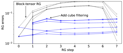
Figure 3: The flow of RG errors before ($\chi=6$) and after entanglement filtering ($\chi=6,\chi_{s}=\chi_{m}=4$), as well as the cube filtering error (the “EF error” in the figure). There are multiple curves of the RG errors for both methods since each RG step contains several projective truncations.

At the critical fixed point, we can linearize the RG map, from whose eigenvalue spectrum the scaling dimensions can be estimated [38, 41]. A salient limitation of a 3D block-tensor map like the HOTRG is that the failure of exhibiting a critical fixed-point tensor [26]. Due to this failure, the estimate of $x_{\epsilon}$ drifts with the RG step for most bond dimensions $\chi\leq 22$ (see Figure 4a, where $x_{\sigma}$ also drifts). Adding the cube filtering allow the RG map exhibit a critical fixed-point tensor; the norm of the difference between two tensors of neighbor RG steps can in general decay down to order $10^{-2}$. Moreover, the estimates of scaling dimensions converge with the RG step. In Figure 4b, the percentages next to the estimates of $x_{\sigma}$ and $x_{\epsilon}$ are relative errors compared with the conformal bootstrap results. At $\chi=6,\chi_{s}=\chi_{m}=4$, the best estimate has relative error $0.1\%$ and $5.3\%$ for $x_{\epsilon}$ and $x_{\sigma}$. We still have not observed a clear improvement of the estimates of $x_{\sigma},x_{\epsilon}$ when $\chi$ increases to 14. The relative errors of the estimates for different $\chi$ are summarized in Table 1. The numerical results can be reproduced using the python codes published at Ref. [42].

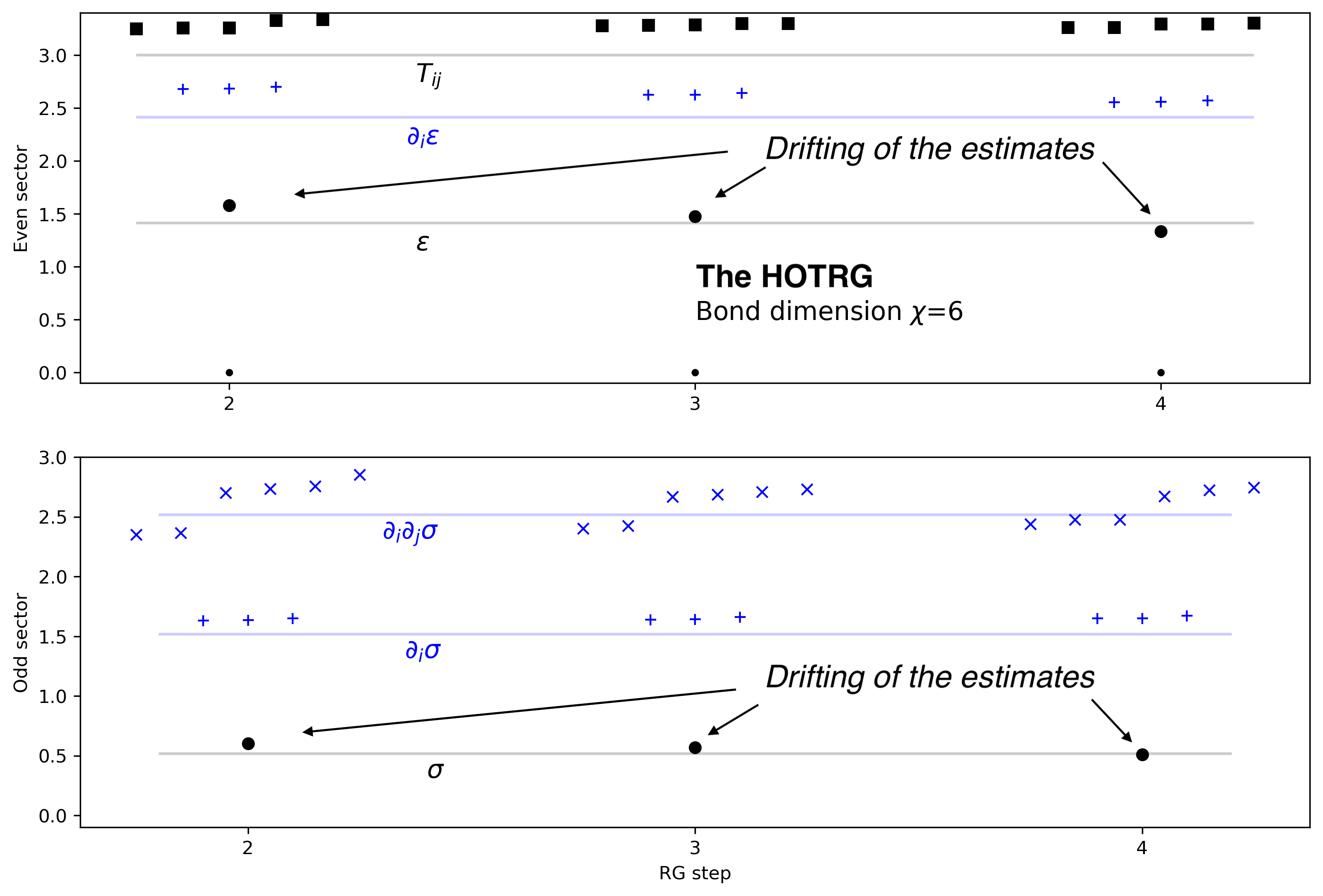
(a) Just block-tensor RG for $\chi=6$

(b) With cube filtering for $\chi=6,\chi_{s}=\chi_{m}=4$

Figure 4: Estimates of scaling dimensions before and after entanglement filtering

Table 1: The estimation errors of $x_{\sigma}$ and $x_{\epsilon}$ versus the bond dimension $\chi$ and hyperparameters $\chi_{s},\chi_{m}$

$\chi,\chi_{s},\chi_{m}$	6,4,4	8,5,8	11,6,8	14,6,10
$x_{\sigma}$	5 $\sim$ 8%	4 $\sim$ 6%	3 $\sim$ 6%	0.4 $\sim$ 0.5%
$x_{\epsilon}$	0.1 $\sim$ 1%	4 $\sim$ 5%	1 $\sim$ 6%	2 $\sim$ 4%

Discussions— The proposed RG has made a solid step towards a systematically-improvable 3D real space RG method. Compared with existing techniques for analyzing critical systems, including Monte Carlo, series expansion and field theory methods, the TNRG can extract much more information. A critical fixed-point tensor, if a TNRG scheme can produce, contains a complete description of a universality class, instead of just a handful of physical observables. The higher scaling dimensions in Figure 4 exhibit conformal tower structure in 3D, which has never been reported numerically until quite recently in a fuzzy sphere construction [43]. Besides the scaling dimensions, operator product expansion coefficients can also be extracted from the fixed-point tensor [44]. Moreover, the method offers a bridge for connecting the RG theory with concepts in conformal field theory. Recently, the relationship between the linearized RG and the dilatation operator has been clarified [41]. It also paves a way for an exact RG treatment of 3D criticality [45, 46, 39] and provides a playground for studying general properties of RG, such as the entropic c-theorems [47, 48, 49, 50]. Due to the high computational costs in 3D, the reachable bond dimension is small, making it harder to demonstrate whether the proposed RG is systematically improvable. The ideas for reducing the computational costs of the 3D TNRG [21, 22, 51] might make the proposed RG a more powerful tool for cracking unsolved problems in 3D classical or (2+1)D quantum criticality.