Physical Layer Security for Continuous-Aperture Array (CAPA) Systems

Abstract

A continuous-aperture array (CAPA)-based secure transmission framework is proposed to enhance physical layer security. Continuous current distributions, or beamformers, are designed to maximize the secrecy transmission rate under a power constraint and to minimize the required transmission power for achieving a specific target secrecy rate. On this basis, the fundamental secrecy performance limits achieved by CAPAs are analyzed by deriving closed-form expressions for the maximum secrecy rate (MSR) and minimum required power (MRP), along with the corresponding optimal current distributions. To provide further insights, asymptotic analyses are performed for the MSR and MRP, which reveals that i) for the MSR, the optimal current distribution simplifies to maximal ratio transmission (MRT) beamforming in the low-SNR regime and to zero-forcing (ZF) beamforming in the high-SNR regime; ii) for the MRP, the optimal current distribution simplifies to ZF beamforming in the high-SNR regime. The derived results are specialized to the typical array structures, e.g., planar CAPAs and planar spatially discrete arrays (SPDAs). The rate and power scaling laws are further analyzed by assuming an infinitely large CAPA. Numerical results demonstrate that: i) the proposed secure continuous beamforming design outperforms MRT and ZF beamforming in terms of both achievable secrecy rate and power efficiency; ii) CAPAs achieve superior secrecy performance compared to conventional SPDAs.

I Introduction

Multiple-antenna technology is a fundamental pillar of modern wireless communication systems. Its core principle is to utilize a larger number of antenna elements in order to enhance spatial degrees of freedom (DoFs) and improve channel capacity [1].

Traditionally, multiple-antenna systems are designed with a spatially discrete topology, where each antenna is represented as an individual point in space. Driven by the benefits of integrating more antennas, the concept of densely packed antenna arrays has gained significant attention in the field of communications. By reducing the spacing between elements within a fixed array aperture, more antennas can be accommodated, thereby enhancing spatial DoFs. This progression has given rise to many state-of-the-art array architectures, such as holographic multiple-input multiple-output (MIMO) systems [2, 3], large intelligent surface [4], dynamic metasurface antennas [5]. In these systems, antenna elements are arranged in an ultra-dense configuration with spacings of less than half a wavelength, leading to improved spectral efficiency [6].

The holy grail of multiple-antenna systems is envisioned as the development of spatially continuous electromagnetic (EM) apertures, referred to as continuous-aperture arrays (CAPAs) [7]. A CAPA operates as a single electrically large-aperture antenna with a continuous current distribution, which comprises a (virtually) infinite number of radiating elements coupled with electronic circuits and a limited number of radio-frequency (RF) chains. On one hand, CAPAs fully utilize the entire aperture surface, which enables significant enhancements in spatial DoFs and array gains. On the other hand, they provide precise control over the amplitude and phase of the current across the aperture’s surface. In summary, CAPAs can leverage spatial resources far more effectively and flexibly than traditional spatially discrete arrays (SPDAs). This capability allows them to approach the theoretical limits of channel capacity, positioning CAPAs as a cornerstone of next-generation wireless communications [7].

Unlike traditional arrays, which are modeled using spatially discrete methods, CAPA-based wireless transmission adopts a fundamentally different approach rooted in the EM field theory. Specifically, while the channels of conventional SPDAs are described using discrete matrices, the spatial response of a CAPA is modeled as a continuous operator in Hilbert space [8]. This discrete-to-continuous transition is not merely a technical adjustment but a paradigm shift in the conceptualization and design of wireless transmission systems [9]. It fundamentally alters the analytical and design frameworks and renders conventional methods developed for SPDAs unsuitable for CAPAs [7]. Therefore, this shift necessitates the development of novel conceptual and mathematical tools tailored to address the continuous EM field interactions in CAPAs [10].

I-A Prior Works

Recently, there has been growing research interest in the design and analysis of CAPA-based wireless communications. In [11], the authors proposed a wavenumber-division multiplexing framework to enable multi-stream data transmission between two linear CAPAs. This concept was extended to CAPA-based multiuser MIMO channels in [12], where a Fourier-based method was developed to maximize the downlink sum-rate by optimizing the current distribution used for modulating RF signals. Building on this approach, [13] further studied beamforming design for uplink multiuser CAPA systems. More recently, [14] and [15] proposed two calculus of variations (CoV)-based approaches for beamforming in unpolarized CAPA-based multiuser channels. Additionally, [16] applied deep learning techniques to design current distributions for multiuser CAPA systems.

In addition to continuous beamforming design, the performance of CAPA-based wireless communication systems has also been analyzed. In [17], the channel capacity between two spherical dielectric CAPAs was studied. The authors of [18] discussed the effective DoFs and capacity between two linear CAPAs. In [19], the Fredholm determinant was utilized to compare the mutual information of CAPA- and SPDA-based MIMO channels, and this analysis was further extended in [20] to incorporate the effects of non-white EM interference. Moreover, [21] analyzed the sum-rate capacity and capacity region of CAPA-based multiuser uplink and downlink channels. Extensions to CAPA-based fading channels were presented in [22] with a focus on the diversity-multiplexing tradeoff in the high signal-to-noise (SNR) region. Additionally, [23] evaluated the signal-to-interference-plus-noise ratio in uplink CAPA systems and proposed an adaptive interference mitigation method. Building on these advancements, a recent study derived the optimal linear receive beamformer for CAPA-based multiuser channels and analyzed the achieved performance in terms of both sum-rate and mean-squared error (MSE) [24].

I-B Motivation and Contributions

The aforementioned works demonstrate the superiority of CAPAs over SPDAs in enhancing wireless communication performance. However, these studies mainly focus on analyzing or optimizing system effectiveness, such as sum-rate [12, 13, 14, 15, 16], or system reliability, such as outage probability [22] and MSE [24]. Beyond these metrics, another critical issue for wireless communication systems is their security. Specifically, the broadcast nature of wireless channels exposes transmitted signals to potentially insecure environments, making them susceptible to interception by eavesdroppers [25]. This vulnerability emphasizes the crucial need for ensuring robust wireless security [25].

In the context of wireless security, secure channel coding has been theoretically proven as an effective approach to achieving nearly 100% secure transmission at the physical layer [25]. This strategy, known as physical layer security (PLS), addresses the limitations of traditional cryptographic methods applied at higher layers (such as the network layer) by eliminating the need for additional spectral resources and reducing signaling overhead [26]. The fundamental model for safeguarding information at the physical layer is Wyner’s wiretap channel [27], which introduced the concept of secrecy transmission rate and secrecy channel capacity—the supremum of the achievable secure coding rate. In recent years, beamforming has been widely recognized as an effective method for enhancing secrecy capacity, thereby improving the PLS of wireless systems [26]. Given that CAPAs are considered a promising architecture for achieving high beamforming gains, their application to PLS is particularly compelling. However, the use of CAPAs to enhance PLS remains underexplored in existing literature, which motivates this work.

This article aims to analyze the fundamental limits of secrecy performance achieved by CAPA-based beamforming. Specifically, we focus on two key aspects: the maximum secrecy rate (MSR) under a given power constraint and the minimum required power (MRP) to achieve a specified secrecy rate target. The main contributions of this work are summarized as follows.

• We propose a CAPA-based transmission framework to enable secure communications with a legitimate user in the presence of an eavesdropper. Leveraging the EM theory and information theory, we introduce continuous operator-based signal and channel models to characterize CAPA-based secure communications. Within this framework, we define two critical metrics to evaluate secrecy performance: the MSR under a given power constraint and the MRP to achieve a specified secrecy rate target.

• For the problem of maximizing the secrecy rate, we derive a closed-form expression for the MSR and the optimal current distribution to achieve it. Additionally, we provide high-SNR and low-SNR approximations of the MSR and prove that the optimal current distribution simplifies to maximal ratio transmission (MRT) beamforming in the low-SNR regime and zero-forcing (ZF) beamforming in the high-SNR regime. Furthermore, we analyze the MSR achieved by a planar CAPA under a line-of-sight (LoS) model. To gain deeper insights, we conduct an asymptotic analysis of the achieved MSR by extending the aperture size to infinity and demonstrate that the asymptotic MSR adheres to the principle of energy conservation.

• For the problem of minimizing the required power to guarantee a target secrecy rate, we derive closed-form expressions for both the optimal current distribution and the MRP. On this basis, we demonstrate that the MRP outperforms that achieved by MRT beamforming and prove that the optimal current distribution simplifies to ZF beamforming when the target secrecy rate becomes infinitely large. Additionally, we derive a closed-form expression for the MRP achieved by a planar CAPA and characterize its asymptotic behavior as the aperture size approaches infinity.

• We provide numerical results to validate the effectiveness of CAPAs in enhancing PLS and demonstrate that: i) increasing the aperture size improves the secrecy performance achieved by CAPA-based secure beamforming; ii) both the MSR and MRP converge to a finite constant as the aperture size of CAPA approaches infinity, which aligns with the principle of energy conservation; iii) the proposed optimal continuous beamformers outperform the MRT and ZF-based schemes in terms of both MSR and MRP; and iv) CAPA yields superior secrecy performance compared to conventional SPDAs.

The remainder of this paper is organized as follows. Section II introduces the CAPA-based secure transmission framework and defines the metrics of MSR and MRP. Sections III and IV analyze the fundamental performance limits of the MSR and MRP achieved by CAPAs, respectively. Section V presents numerical results to validate the theoretical findings. Finally, Section VI concludes the paper.

Notations

Throughout this paper, scalars, vectors, and matrices are denoted by non-bold, bold lower-case, and bold upper-case letters, respectively. For the matrix $\mathbf{A}$, ${\mathbf{A}}^{\mathsf{T}}$, ${\mathbf{A}}^{*}$ and ${\mathbf{A}}^{\mathsf{H}}$ denote its transpose, conjugate and transpose conjugate, respectively. For the square matrix $\mathbf{B}$, $\det(\mathbf{B})$ denotes its determinant. The notations $\lvert a\rvert$ and $\lVert\mathbf{a}\rVert$ denote the magnitude and norm of scalar $a$ and vector $\mathbf{a}$, respectively. The set $\mathbbmss{R}$ and $\mathbbmss{C}$ stand for the real and complex spaces, respectively, and notation $\mathbbmss{E}\{\cdot\}$ represents mathematical expectation. And we generally reserve the symbols $I(\cdot)$ for mutual information and $H(\cdot)$ for entropy. Finally, ${\mathcal{CN}}({\bm{\mu}},\mathbf{X})$ is used to denote the circularly-symmetric complex Gaussian distribution with mean $\bm{\mu}$ and covariance matrix $\mathbf{X}$.

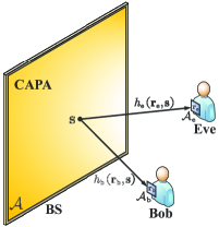
Figure 1: Illustration of a CAPA-based wiretap channel.

II System Model

As illustrated in Figure 1, we consider a wiretap channel consisting of a base station (BS), a legitimate user (Bob, denoted as $\rm{b}$), and an eavesdropper (Eve, denoted as $\rm{e}$). Each entity is equipped with a CAPA. Let $\mathcal{A}\subseteq{\mathbbmss{R}}^{3\times 1}$ represent the aperture of the CAPA at the BS, with its size given by $\lvert\mathcal{A}\rvert=\int_{\mathcal{A}}{\rm{d}}{\mathbf{s}}$. Moreover, let ${\mathcal{A}}_{k}\subseteq{\mathbbmss{R}}^{3\times 1}$ denote the aperture of the CAPA at each user $k\in\{\rm{b},\rm{e}\}$, with the aperture size $\lvert\mathcal{A}_{k}\rvert=\int_{{\mathcal{A}}_{k}}{\rm{d}}{\mathbf{r}}$. It is assumed that the aperture size of each user is significantly smaller than that of the BS, i.e., $\lvert\mathcal{A}\rvert\gg\lvert\mathcal{A}_{k}\rvert$ ($\forall k$). Moreover, both Bob and Eve are assumed to have complete channel state information (CSI) regarding their respective effective channels. It is further assumed that Eve is a registered user, and thus, the BS obtains the CSI for both Eve and Bob during the channel training phase [28]. Under these conditions, Eve is expected to receive the common messages broadcast across the network but remain uninformed about the confidential messages intended solely for Bob.

II-A CAPA-Based Transmission

The BS intends to transmit a confidential message $W$ to Bob over $N$ channel uses, and ensures that it remains secret from Eve. To achieve this, the BS first encodes the confidential message $W$ into the codeword $[s(1),\ldots,s(N)]$ using a properly designed encoder [29]. The encoded symbols are Gaussian distributed with zero mean and unit variance, i.e., $s(n)\sim{\mathcal{CN}}(0,1)$ for $n\in{\mathcal{N}}\triangleq\{1,\ldots,N\}$.

Next, the BS maps the encoded symbols over the time interval $n\in{\mathcal{N}}$, i.e., $s(n)$, into the transmit signal $x(\mathbf{s},n)\in{\mathbbmss{C}}$ by utilizing a source current $j({\mathbf{s}})$ for $\mathbf{s}\in\mathcal{A}$. This signal is radiated towards Bob, while also being overheard by Eve. The transmit signal at the $n$th time interval is given by

$${x}(\mathbf{s},n)=j({\mathbf{s}})s(n),~n\in{\mathcal{N}},$$ (1)

where the source current is subject to the power constraint $\int_{\mathcal{A}}\lvert j({\mathbf{s}})\rvert^{2}{\rm{d}}{\mathbf{s}}\leq P$. Therefore, the electric field excited by ${x}(\mathbf{s},n)$ at point $\mathbf{r}\in\mathcal{A}_{k}$ can be written as follows [30]:

$$e_{k}(\mathbf{r},n) =\int_{{\mathcal{A}}}h_{k}(\mathbf{r},{\mathbf{s}}){x}({\mathbf{s}},n){\rm{d}}{\mathbf{s}}$$ (2a)

$$=s(n)\int_{{\mathcal{A}}}h_{k}(\mathbf{r},{\mathbf{s}})j({\mathbf{s}}){\rm{d}}{\mathbf{s}},$$ (2b)

where $h_{k}(\mathbf{r},{\mathbf{s}})$ denotes user $k$’s spatial response from $\mathbf{s}$ to $\mathbf{r}$.

The total observation of user $k$ at point $\mathbf{r}\in{\mathcal{A}}_{k}$ is the sum of the information-carrying electric field $e_{k}(\mathbf{r},n)$ and a random noise field $z_{k}(\mathbf{r},n)$, i.e.,

$$y_{k}(\mathbf{r},n) =e_{k}(\mathbf{r},n)+z_{k}(\mathbf{r},n)$$ (3a)

$$=s(n)\int_{{\mathcal{A}}}h_{k}(\mathbf{r},{\mathbf{s}})j({\mathbf{s}}){\rm{d}}{\mathbf{s}}+z_{k}(\mathbf{r},n),$$ (3b)

where $z_{k}(\mathbf{r},n)$ denotes the $n$th sample of additive white Gaussian noise (AWGN) at ${\mathbf{r}}$ with mean zero and variance (noise power) $\sigma_{k}^{2}$, i.e., $z_{k}(\mathbf{r},n)\sim{\mathcal{CN}}(0,\sigma_{k}^{2})$. The SNR of user $k$ for decoding $s(n)$ is given by [21]

$$\gamma_{k} =\frac{{\mathbbmss{E}}\{\lvert s(n)\rvert^{2}\}\left\lvert\int_{\mathcal{A}_{k}}\int_{{\mathcal{A}}}h_{k}(\mathbf{r},{\mathbf{s}})j({\mathbf{s}}){\rm{d}}{\mathbf{s}}{\rm{d}}{\mathbf{r}}\right\rvert^{2}}{\int_{\mathcal{A}_{k}}{\mathbbmss{E}}\{\lvert z_{k}(\mathbf{r},n)\rvert^{2}\}{\rm{d}}{\mathbf{r}}}$$ (4a)

$$=\frac{1}{\sigma_{k}^{2}\lvert\mathcal{A}_{k}\rvert}{\left\lvert\int_{\mathcal{A}_{k}}\int_{{\mathcal{A}}}h_{k}(\mathbf{r},{\mathbf{s}})j({\mathbf{s}}){\rm{d}}{\mathbf{s}}{\rm{d}}{\mathbf{r}}\right\rvert^{2}}.$$ (4b)

Given that the aperture size of each user is typically on the order of the wavelength, it is significantly smaller than both the propagation distance and the size of the BS aperture. Therefore, the variations in the channel response across the receive aperture are negligible, which yields

$$h_{k}(\mathbf{r},{\mathbf{s}})\approx h_{k}(\mathbf{r}_{k},{\mathbf{s}})\triangleq h_{k}(\mathbf{s}).$$ (5)

As a results, we can approximate (4b) as follows:

$$\gamma_{k}\approx\frac{\lvert\mathcal{A}_{k}\rvert}{\sigma_{k}^{2}}{\left\lvert\int_{{\mathcal{A}}}h_{k}({\mathbf{s}})j({\mathbf{s}}){\rm{d}}{\mathbf{s}}\right\rvert^{2}}.$$ (6)

II-B Secure Transmission

Bob makes an estimate $\hat{W}$ of $W$ based on the received output ${\mathbf{y}}_{\rm{b}}=[{{y}}_{\rm{b}}(1),\ldots,{{y}}_{\rm{b}}(N)]^{\mathsf{T}}$ from its channel, resulting in a block error rate $\epsilon_{N}=\Pr(W\neq\hat{W})$. The confidential message $W$ is also the input to Eve’s channel, and Eve has an average residual uncertainty $H(W|{\mathbf{y}}_{\rm{e}})$ after observing the output ${\mathbf{y}}_{\rm{e}}=[{{y}}_{\rm{e}}(1),\ldots,{{y}}_{\rm{e}}(N)]^{\mathsf{T}}$. Defining the transmission rate as $\mathcal{R}_{N}\triangleq H(W)/N$, and the fractional equivocation of Eve as $\Delta_{N}\triangleq H(W|{\mathbf{y}}_{\rm{e}})/H(W)$, the information-theoretic limits of secure transmission is described as follows [29].

Secure Coding Theorem

For any transmission rate ${\mathcal{R}}<{\mathcal{R}}_{j(\mathbf{s})}\triangleq\max\{\log_{2}(1+\gamma_{\rm{b}})-\log_{2}(1+\gamma_{\rm{e}}),0\}$, there exists an encoder-decoder pair such that as $N\rightarrow\infty$, the rate $\mathcal{R}_{N}\rightarrow\mathcal{R}$, the equivocation $\Delta_{N}\rightarrow 1$, and the error probability $\epsilon_{N}\rightarrow 0$.

We comment that $\Delta_{N}\rightarrow 1$ is equivalent to $H(W|{\mathbf{y}}_{\rm{e}})\rightarrow H(W)$, or $I(W;{\mathbf{y}}_{\rm{e}})=H(W)-H(W|{\mathbf{y}}_{\rm{e}})\rightarrow 0$, meaning that Eve is unable to extract any information about the confidential message $W$. The above statements suggest that the maximum secure transmission rate for a given source current distribution $j({\mathbf{s}})$ is ${\mathcal{R}}_{j(\mathbf{s})}$. Below this rate, Bob is able to recover the confidential message with arbitrary precision, while Eve cannot obtain any information from $W$.

Since the secrecy rate ${\mathcal{R}}_{j(\mathbf{s})}$ is a function of the current distribution $j({\mathbf{s}})$, we consider two key metrics to characterize the secrecy performance limits of the considered system.

II-B1 Maximum Secrecy Rate

The MSR, subject to the power budget $P$, is defined as follows:

$${\mathcal{R}}_{\star} \triangleq\max_{\int_{\mathcal{A}}\lvert j({\mathbf{s}})\rvert^{2}{\rm{d}}{\mathbf{s}}\leq P}{\mathcal{R}}_{j(\mathbf{s})}$$ (7a)

$$=\max_{\int_{\mathcal{A}}\lvert j({\mathbf{s}})\rvert^{2}{\rm{d}}{\mathbf{s}}\leq P}\max\left\{\log_{2}\left(\frac{1+\gamma_{\rm{b}}}{1+\gamma_{\rm{e}}}\right),0\right\}.$$ (7b)

II-B2 Minimum Required Transmit Power

Another metric of interest is the MRP to ensure a target secrecy rate ${\mathsf{R}}_{0}>0$, which is defined as follows:

$${\mathcal{P}}_{\star} \triangleq\min_{{\mathcal{R}}_{j(\mathbf{s})}\geq{\mathsf{R}}_{0}}{\int_{\mathcal{A}}\lvert j({\mathbf{s}})\rvert^{2}{\rm{d}}{\mathbf{s}}}$$ (8a)

$$=\min_{\log_{2}\left(\frac{1+\gamma_{\rm{b}}}{1+\gamma_{\rm{e}}}\right)\geq{\mathsf{R}}_{0}}{\int_{\mathcal{A}}\lvert j({\mathbf{s}})\rvert^{2}{\rm{d}}{\mathbf{s}}}.$$ (8b)

Achieving the MSR or the MRP are fundamental objectives in secure transmission. The MSR represents the highest rate at which data can be securely transmitted, while the MRP indicates the minimum power needed to achieve a desired level of security. In the following sections, we derive closed-form expressions for ${\mathcal{R}}_{\star}$ and ${\mathcal{P}}_{\star}$, as defined in (7b) and (8b), respectively, and analyze these two key metrics.

III Analysis of the Maximum Secrecy Rate

In this section, we analyze the MSR by deriving its close-form expression and the associate current distribution.

III-A Problem Reformulation

Based on (6) and (7b), the problem of secrecy rate maximization can be formulated as follows:

$$\max_{\int_{\mathcal{A}}{\left|j(\mathbf{s})\right|^{2}}\mathrm{d}\mathbf{s}\leq P}\frac{1+\frac{\lvert\mathcal{A}_{\mathrm{b}}\rvert}{\sigma_{\mathrm{b}}^{2}}\left|\int_{\mathcal{A}}{h_{\mathrm{b}}}(\mathbf{s})j(\mathbf{s})\mathrm{d}\mathbf{s}\right|^{2}}{1+\frac{\lvert\mathcal{A}_{\mathrm{e}}\rvert}{\sigma_{\mathrm{e}}^{2}}\left|\int_{\mathcal{A}}{h_{\mathrm{e}}}(\mathbf{s})j(\mathbf{s})\mathrm{d}\mathbf{s}\right|^{2}}.$$ (9)

According to the monotonicity of function $f(x)=\frac{1+ax}{1+bx}$ for $x>0$ and $a>b>0$, it can be easily shown that the optimal $j(\mathbf{s})$ satisfies $\int_{\mathcal{A}}{\left|j(\mathbf{s})\right|^{2}}\mathrm{d}\mathbf{s}=P$. By defining $\overline{\gamma}_{k}\triangleq\frac{P\lvert\mathcal{A}_{k}\rvert}{{\sigma}_{k}^{2}}$ for $k\in\{\rm{b},\rm{e}\}$ and $u(\mathbf{s})\triangleq\frac{j(\mathbf{s})}{\sqrt{P}}$, we rewrite (9) as follows:

$$\max_{\int_{\mathcal{A}}{\left|u(\mathbf{s})\right|^{2}}\mathrm{d}\mathbf{s}=1}\frac{1+\overline{\gamma}_{\mathrm{b}}\left|\int_{\mathcal{A}}h_{\mathrm{b}}(\mathbf{s})u(\mathbf{s})\mathrm{d}\mathbf{s}\right|^{2}}{1+\overline{\gamma}_{\mathrm{e}}\left|\int_{\mathcal{A}}{h_{\mathrm{e}}}(\mathbf{s})u(\mathbf{s})\mathrm{d}\mathbf{s}\right|^{2}}.$$ (10)

Furthermore, for $k\in\{\rm{b},\rm{e}\}$, it holds that

$$1=\int_{\mathcal{A}}{\left\lvert u(\mathbf{s})\right\rvert^{2}}\mathrm{d}\mathbf{s}\overset{\clubsuit}{=}\int_{\mathcal{A}}\int_{\mathcal{A}}u(\mathbf{s})\delta(\mathbf{s}-\mathbf{s}^{\prime})u^{*}(\mathbf{s}^{\prime})\mathrm{d}\mathbf{s}\mathrm{d}\mathbf{s}^{\prime},$$

$$\left\lvert\int_{\mathcal{A}}{h_{k}(\mathbf{s})u(\mathbf{s})}\mathrm{d}\mathbf{s}\right\rvert^{2}=\int_{\mathcal{A}}\int_{\mathcal{A}}{{u(\mathbf{s})h_{k}(\mathbf{s})h_{k}^{*}(\mathbf{s}^{\prime})u^{*}(\mathbf{s}^{\prime})\mathrm{d}\mathbf{s}\mathrm{d}\mathbf{s}^{\prime}}},$$

where $\delta(\cdot)$ is the Dirac delta function, step $\clubsuit$ follows from the fact that $\int_{{\mathcal{A}}}\delta({\mathbf{x}}-{\mathbf{x}}_{0})f(\mathbf{x}){\rm{d}}{\mathbf{x}}=f({\mathbf{x}}_{0})$ with $f(\cdot)$ being an arbitrary function defined on ${\mathcal{A}}$. Taken together, we obtain

$$1+\overline{\gamma}_{k}\left\lvert\int_{\mathcal{A}}{h_{k}(\mathbf{s})u(\mathbf{s})}\mathrm{d}\mathbf{s}\right\rvert^{2}\!=\int_{\mathcal{A}}\int_{\mathcal{A}}{{u(\mathbf{s})A_{k}(\mathbf{s},\mathbf{s}^{\prime})}}u^{*}(\mathbf{s}^{\prime})\mathrm{d}\mathbf{s}\mathrm{d}\mathbf{s}^{\prime},$$

where $A_{k}(\mathbf{s},\mathbf{s}^{\prime})\triangleq\delta(\mathbf{s}-\mathbf{s}^{\prime})+\overline{\gamma}_{k}h_{k}(\mathbf{s})h_{k}^{*}(\mathbf{s}^{\prime})$. Consequently, the objective function in (10) equals the generalized Rayleigh quotient given as follows:

$${\mathsf{RQ}}(u(\mathbf{s}))\triangleq\frac{\int_{\mathcal{A}}\int_{\mathcal{A}}{u(\mathbf{s})A_{\rm{b}}(\mathbf{s},\mathbf{s}^{\prime})}u^{*}(\mathbf{s}^{\prime})\mathrm{d}\mathbf{s}\mathrm{d}\mathbf{s}^{\prime}}{\int_{\mathcal{A}}{\int_{\mathcal{A}}{u(\mathbf{s})A_{\rm{e}}(\mathbf{s},\mathbf{s}^{\prime})}}u^{*}(\mathbf{s}^{\prime})\mathrm{d}\mathbf{s}\mathrm{d}\mathbf{s}^{\prime}}.$$ (11)

We note that the value of ${\mathsf{RQ}}(u(\mathbf{s}))$ is not affected by the norm of $u(\mathbf{s})$, i.e., $\int_{\mathcal{A}}{\left|u(\mathbf{s})\right|^{2}\mathrm{d}\mathbf{s}}$. Therefore, the optimization problem in (9) is equivalent to the following one:

$$\max_{u(\mathbf{s})}{\mathsf{RQ}}(u(\mathbf{s}))\Leftrightarrow\eqref{CAP_MISOSE_Problem_1}.$$ (12)

To solve problem (12), we define two functions as follows:

$$Q\left(\mathbf{s},\mathbf{s}^{\prime}\right) \triangleq\delta(\mathbf{s}-\mathbf{s}^{\prime})+\mu h_{\mathrm{e}}(\mathbf{s})h_{\mathrm{e}}^{*}(\mathbf{s}^{\prime}),$$ (13)

$$\hat{Q}\left(\mathbf{s},\mathbf{s}^{\prime}\right) \triangleq\delta(\mathbf{s}-\mathbf{s}^{\prime})-\frac{\mu}{1+\mu g_{\mathrm{e}}}h_{\mathrm{e}}(\mathbf{s})h_{\mathrm{e}}^{*}(\mathbf{s}^{\prime}),$$ (14)

where $\mu=-\frac{1}{g_{\mathrm{e}}}\pm\frac{1}{g_{\mathrm{e}}\sqrt{1+\overline{\gamma}_{\mathrm{e}}g_{\mathrm{e}}}}$, and $g_{\mathrm{e}}=\int_{\mathcal{A}}{\left|h_{\mathrm{e}}(\mathbf{s})\right|^{2}\mathrm{d}\mathbf{s}}$ represents the channel gain for Eve. Then, the following lemmas can be found.

Lemma 1.

Given $h_{\mathrm{e}}(\mathbf{s})$, $Q\left(\mathbf{s},\mathbf{s}^{\prime}\right)$ and $\hat{Q}\left(\mathbf{s},\mathbf{s}^{\prime}\right)$ are mutually invertible, which satisfy

$$\begin{split}\int_{\mathcal{A}}Q\left(\mathbf{s},\mathbf{s}_{1}\right)\hat{Q}\left(\mathbf{s}_{1},\mathbf{s}^{\prime}\right){\rm{d}}\mathbf{s}_{1}&=\int_{\mathcal{A}}\hat{Q}\left(\mathbf{s},\mathbf{s}_{1}\right)Q\left(\mathbf{s}_{1},\mathbf{s}^{\prime}\right){\rm{d}}\mathbf{s}_{1}\\ &=\delta(\mathbf{s}-\mathbf{s}^{\prime}).\end{split}$$ (15)

Proof:

Please refer to Appendix -A for more details. ∎

Lemma 2.

Given $h_{\mathrm{e}}(\mathbf{s})$, it holds that

$$\begin{split}\int_{\mathcal{A}}\!\int_{\mathcal{A}}\!Q\left(\mathbf{s}_{1},\mathbf{s}\right)A_{\rm{e}}(\mathbf{s},\mathbf{s}^{\prime})Q\left(\mathbf{s}^{\prime},\mathbf{s}_{1}^{\prime}\right){\rm{d}}\mathbf{s}{\rm{d}}\mathbf{s}^{\prime}=\delta(\mathbf{s}_{1}-\mathbf{s}_{1}^{\prime}).\end{split}$$ (16)

Proof:

Please refer to Appendix -B for more details. ∎

Motivated by the results in Lemma 2, we define the following function:

$${\nu}(\mathbf{s}_{1})\triangleq\int_{{\mathcal{A}}}u({\mathbf{s}})\hat{Q}\left(\mathbf{s},\mathbf{s}_{1}\right){\rm{d}}{\mathbf{s}},$$ (17)

which, together with (15), yields

$$\int_{\mathcal{A}}{\nu}(\mathbf{s}_{1})Q\left(\mathbf{s}_{1},\mathbf{s}^{\prime}\right){\rm{d}}{\mathbf{s}}_{1} =\int_{{\mathcal{A}}}\int_{\mathcal{A}}u({\mathbf{s}})\hat{Q}\left(\mathbf{s},\mathbf{s}_{1}\right)Q\left(\mathbf{s}_{1},\mathbf{s}^{\prime}\right){\rm{d}}{\mathbf{s}}$$

$$=\int_{\mathcal{A}}u({\mathbf{s}})\delta(\mathbf{s}-\mathbf{s}^{\prime}){\rm{d}}{\mathbf{s}}=u(\mathbf{s}^{\prime}).$$ (18)

The above arguments imply that $u(\cdot)$ and ${\nu}(\cdot)$ can be mutually transformed. Therefore, we can transform the variable to be optimized in (12) from $u(\mathbf{s})$ to ${\nu}(\mathbf{s})$ by setting $u(\mathbf{s})=\int_{\mathcal{A}}{\nu}(\mathbf{s}_{1})Q\left({\mathbf{s}}_{1},\mathbf{s}\right){\rm{d}}{\mathbf{s}}_{1}$. As a result, the denominator of (11) can be written as follows:

$$\begin{split}&\int_{\mathcal{A}}{\int_{\mathcal{A}}{u(\mathbf{s})A_{\rm{e}}(\mathbf{s},\mathbf{s}^{\prime})}}u^{*}(\mathbf{s}^{\prime})\mathrm{d}\mathbf{s}\mathrm{d}\mathbf{s}^{\prime}\\ &=\int_{\mathcal{A}}\int_{\mathcal{A}}{\nu}(\mathbf{s}_{1}){\hat{E}}(\mathbf{s}_{1},\mathbf{s}_{1}^{\prime}){\nu}^{*}(\mathbf{s}_{1}^{\prime})\mathrm{d}\mathbf{s}_{1}\mathrm{d}\mathbf{s}_{1}^{\prime},\end{split}$$ (19)

where ${\hat{E}}(\mathbf{s}_{1},\mathbf{s}_{1}^{\prime})=\int_{\mathcal{A}}\int_{\mathcal{A}}Q\left({\mathbf{s}}_{1},\mathbf{s}\right)A_{\rm{e}}(\mathbf{s},\mathbf{s}^{\prime})Q^{*}\left({\mathbf{s}}_{1}^{\prime},\mathbf{s}^{\prime}\right)\mathrm{d}\mathbf{s}\mathrm{d}\mathbf{s}^{\prime}$. According to the definition of $Q(\cdot,\cdot)$, we have $Q^{*}\left({\mathbf{s}}_{1}^{\prime},\mathbf{s}^{\prime}\right)=Q\left(\mathbf{s}^{\prime},{\mathbf{s}}_{1}^{\prime}\right)$, which, together with Lemma 1, yields ${\hat{E}}(\mathbf{s}_{1},\mathbf{s}_{1}^{\prime})=\delta(\mathbf{s}_{1},\mathbf{s}_{1}^{\prime})$. It follows that

$$\int_{\mathcal{A}}\int_{\mathcal{A}}{\nu}(\mathbf{s}_{1})\delta(\mathbf{s}_{1},\mathbf{s}_{1}^{\prime}){\nu}^{*}(\mathbf{s}_{1}^{\prime})\mathrm{d}\mathbf{s}_{1}\mathrm{d}\mathbf{s}_{1}^{\prime}=\int_{\mathcal{A}}{\left|\nu(\mathbf{s}_{1})\right|^{2}\mathrm{d}\mathbf{s}_{1}}.$$ (20)

Taken together, we transform problem (12) into the following equivalent form:

$$\max_{\nu(\mathbf{s}_{1})}\frac{\int_{\mathcal{A}}{\int_{\mathcal{A}}}\nu(\mathbf{s}_{1})B(\mathbf{s}_{1},\mathbf{s}_{1}^{\prime})\nu^{*}(\mathbf{s}_{1}^{\prime})\mathrm{d}\mathbf{s}_{1}\mathrm{d}\mathbf{s}_{1}^{\prime}}{\int_{\mathcal{A}}{\left|\nu(\mathbf{s}_{1})\right|^{2}}\mathrm{d}\mathbf{s}_{1}},$$ (21)

where

$$B(\mathbf{s}_{1},\mathbf{s}_{1}^{\prime})=\int_{\mathcal{A}}\int_{\mathcal{A}}Q\left(\mathbf{s}_{1},\mathbf{s}\right)A_{\rm{b}}(\mathbf{s},\mathbf{s}^{\prime})Q\left(\mathbf{s}^{\prime},\mathbf{s}_{1}^{\prime}\right){\rm{d}}\mathbf{s}{\rm{d}}\mathbf{s}^{\prime}.$$ (22)

Note that the objective function of problem (21) is not influenced by the norm of $\nu(\mathbf{s}_{1})$, i.e., $\int_{\mathcal{A}}{\left|\nu(\mathbf{s}_{1})\right|^{2}\mathrm{d}\mathbf{s}_{1}}$. Thus, problem (21) can be simplified by removing the denominator term therein. The final results are given as follows.

Theorem 1.

The secrecy rate maximization problem defined in (9) is equivalent to the following:

$$\nu^{\star}(\mathbf{s}_{1})=\operatorname*{argmax}_{\nu(\mathbf{s}_{1})}\int_{\mathcal{A}}{\int_{\mathcal{A}}}{\nu}(\mathbf{s}_{1})B(\mathbf{s}_{1},\mathbf{s}_{1}^{\prime}){\nu}^{*}(\mathbf{s}_{1}^{\prime})\mathrm{d}\mathbf{s}_{1}\mathrm{d}\mathbf{s}_{1}^{\prime}.$$ (23)

After obtaining $\nu^{\star}(\mathbf{s}_{1})$, the source current distribution that maximizes the secrecy rate can be calculated as follows:

$$j_{\mathsf{msr}}\left(\mathbf{s}\right)=\frac{\sqrt{P}\int_{\mathcal{A}}{\nu}^{\star}(\mathbf{s}_{1})Q\left({\mathbf{s}}_{1},\mathbf{s}\right){\rm{d}}{\mathbf{s}}_{1}}{\sqrt{\int_{{\mathcal{A}}}\lvert\int_{\mathcal{A}}{\nu}^{\star}(\mathbf{s}_{1})Q\left({\mathbf{s}}_{1},\mathbf{s}\right){\rm{d}}{\mathbf{s}}_{1}\rvert^{2}{\rm{d}}{\mathbf{s}}}}.$$ (24)

Proof:

The results follow directly from using (17). ∎

III-B Maximum Secrecy Rate & Optimal Current Distribution

In this subsection, we aim to solve problem (23) and derive closed-form expressions for the optimal current distribution and the achieved MSR.

III-B1 Maximum Secrecy Rate

The results in Theorem 1 suggest that the optimal solution to problem (23), i.e., the rate-optimal source current distribution, corresponds to the principal eigenfunction of the operator $B(\mathbf{s}_{1},\mathbf{s}_{1}^{\prime})$. Furthermore, the optimal objective value of problem (23) is given by the principal eigenvalue of $B(\mathbf{s}_{1},\mathbf{s}_{1}^{\prime})$. Therefore, we have

$${\mathcal{R}}_{\star}=\max_{\int_{\mathcal{A}}\lvert j({\mathbf{s}})\rvert^{2}{\rm{d}}{\mathbf{s}}\leq P}{\mathcal{R}}_{j(\mathbf{s})}=\log_{2}(\lambda_{B}^{\max}),$$ (25)

where $\lambda_{B}^{\max}$ denotes the principal eigenvalue of $B(\mathbf{s}_{1},\mathbf{s}_{1}^{\prime})$.

To calculate each eigenvalue $\lambda_{B}$ of $B(\mathbf{s}_{1},\mathbf{s}_{1}^{\prime})$, we need to solve the following characteristic equation:

$$\det(B(\mathbf{s}_{1},\mathbf{s}_{1}^{\prime})-\lambda_{B}\delta(\mathbf{s}_{1}-\mathbf{s}_{1}^{\prime}))=0,$$ (26)

where $\det(\cdot)$ here is utilized to calculate the Fredholm determinant of the operator $B(\mathbf{s}_{1},\mathbf{s}_{1}^{\prime})-\lambda_{B}\delta(\mathbf{s}_{1}-\mathbf{s}_{1}^{\prime})\triangleq{\hat{B}}(\mathbf{s}_{1},\mathbf{s}_{1}^{\prime})$, i.e., the product of all its eigenvalues [31]. Since directly solving equation (26) is challenging, we define

$$C(\mathbf{s}_{2},\mathbf{s}_{2}^{\prime})\triangleq \int_{\mathcal{A}}{\int_{\mathcal{A}}}\hat{Q}(\mathbf{s}_{2},\mathbf{s}_{1}){\hat{B}}(\mathbf{s}_{1},\mathbf{s}_{1}^{\prime})\hat{Q}(\mathbf{s}^{\prime}_{1},\mathbf{s}^{\prime}_{2})\mathrm{d}\mathbf{s}_{1}\mathrm{d}\mathbf{s}_{1}^{\prime}.$$ (27)

Then, the following lemma can be concluded.

Lemma 3.

Given $h_{\mathrm{b}}(\mathbf{s})$ and $h_{\mathrm{e}}(\mathbf{s})$, it holds that

$$\begin{split}C(\mathbf{s}_{2},\mathbf{s}_{2}^{\prime})&=\overline{\gamma}_{\mathrm{b}}h_{\mathrm{b}}(\mathbf{s}_{2})h_{\mathrm{b}}^{*}(\mathbf{s}_{2}^{\prime})-\lambda_{B}\overline{\gamma}_{\mathrm{e}}h_{\mathrm{e}}(\mathbf{s}_{2})h_{\mathrm{e}}^{*}(\mathbf{s}_{2}^{\prime})\\ &+(1-\lambda_{B})\delta(\mathbf{s}_{2}-\mathbf{s}_{2}^{\prime}).\end{split}$$ (28)

Proof:

Please refer to Appendix -C for more details. ∎

According to Lemma 2, $\hat{Q}(\cdot,\cdot)$ is an invertible operator. Consequently, we have

$$\det({\hat{B}}(\mathbf{s}_{1},\mathbf{s}_{1}^{\prime}))=0\Leftrightarrow\det(C(\mathbf{s}_{2},\mathbf{s}_{2}^{\prime}))=0,$$ (29)

which means that we can equivalently transform equation (26) to the following equation:

$$\det(C(\mathbf{s}_{2},\mathbf{s}_{2}^{\prime}))=0.$$ (30)

Note that the operator $C(\mathbf{s}_{2},\mathbf{s}_{2}^{\prime})$ is Hermitian, i.e., $C(\mathbf{s}_{2},\mathbf{s}_{2}^{\prime})=C^{*}(\mathbf{s}_{2}^{\prime},\mathbf{s}_{2})$, and thus its determinant is equal to the product of the eigenvalues, i.e., $\det(C(\mathbf{s}_{2},\mathbf{s}_{2}^{\prime}))=\prod_{i=1}^{\infty}{\lambda_{C,i}}$ with $\lambda_{C,i}$ being the $i$th eigenvalue of $C(\mathbf{s}_{2},\mathbf{s}_{2}^{\prime})$. Consequently, we can rewrite (30) as follows:

$$\det(C(\mathbf{s}_{2},\mathbf{s}_{2}^{\prime}))=\prod\nolimits_{i=1}^{\infty}{\lambda_{C,i}}=0.$$ (31)

By observing the mathematical structure of $C(\mathbf{s}_{2},\mathbf{s}_{2}^{\prime})$ given in (28), we conclude the following lemma.

Lemma 4.

Given $h_{\mathrm{b}}(\mathbf{s})$ and $h_{\mathrm{e}}(\mathbf{s})$, the eigenvalues of $C(\mathbf{s}_{2},\mathbf{s}_{2}^{\prime})$ are given as follows:

$$\lambda_{C,1}=\xi_{1}-\lambda_{B}+1,\ \lambda_{C,2}=\xi_{2}-\lambda_{B}+1,$$ (32a)

$$\lambda_{C,3}=\ldots=\lambda_{C,\infty}=-\lambda_{B}+1.$$ (32b)

Here,

$$\xi_{1} =\frac{\Delta+\sqrt{\Delta^{2}+4\lambda_{B}\overline{\gamma}_{\mathrm{b}}\overline{\gamma}_{\mathrm{e}}g_{\mathrm{b}}g_{\mathrm{e}}(1-\overline{\rho})}}{2},$$ (33a)

$$\xi_{2} =\frac{\Delta-\sqrt{\Delta^{2}+4\lambda_{B}\overline{\gamma}_{\mathrm{b}}\overline{\gamma}_{\mathrm{e}}g_{\mathrm{b}}g_{\mathrm{e}}(1-\overline{\rho})}}{2},$$ (33b)

where $\Delta=\overline{\gamma}_{\mathrm{b}}g_{\mathrm{b}}-\lambda_{B}\overline{\gamma}_{\mathrm{e}}g_{\mathrm{e}}$, $g_{\mathrm{b}}=\int_{\mathcal{A}}{\left|h_{\mathrm{b}}(\mathbf{s})\right|^{2}\mathrm{d}\mathbf{s}}$ represents the channel gain for Bob, $\overline{\rho}=\frac{\left|\rho\right|^{2}}{g_{\mathrm{b}}g_{\mathrm{e}}}\in[0,1)$ denotes the channel correlation factor between Bob and Eve, with $\rho\triangleq\int_{\mathcal{A}}{h_{\mathrm{b}}(\mathbf{s})h_{\mathrm{e}}^{*}(\mathbf{s})\mathrm{d}\mathbf{s}}$.

Proof:

Please refer to Appendix -D for more details. ∎

Substituting (32) into (31) gives

$$(\xi_{1}-\lambda_{B}+1)(\xi_{2}-\lambda_{B}+1)\prod\nolimits_{i=3}^{\infty}(-\lambda_{B}+1)=0.$$ (34)

By solving the above equation with respect to $\lambda_{B}$, we can obtain all the eigenvalues of $B(\mathbf{s}_{1},\mathbf{s}_{1}^{\prime})$. The corresponding results are summarized as follows.

Theorem 2.

Given $h_{\mathrm{b}}(\mathbf{s})$ and $h_{\mathrm{e}}(\mathbf{s})$, the principal eigenvalue of operator $B(\mathbf{s}_{1},\mathbf{s}_{1}^{\prime})$ can be expressed as follows:

$$\lambda_{B}^{\max}=1+\frac{\overline{\gamma}_{\mathrm{b}}g_{\mathrm{b}}\left(1+\overline{\gamma}_{\mathrm{e}}g_{\mathrm{e}}\left(1-\overline{\rho}\right)\right)}{1+\overline{\gamma}_{\mathrm{e}}g_{\mathrm{e}}}.$$ (35)

Proof:

Please refer to Appendix -E for more details. ∎

Consequently, we derive the closed-form expression for the MSR in the following theorem.

Theorem 3.

Given $h_{\mathrm{b}}(\mathbf{s})$ and $h_{\mathrm{e}}(\mathbf{s})$, the MSR is given by

$${\mathcal{R}}_{\star}=\log_{2}\left(1+\frac{\overline{\gamma}_{\mathrm{b}}g_{\mathrm{b}}\left(1+\overline{\gamma}_{\mathrm{e}}g_{\mathrm{e}}\left(1-\overline{\rho}\right)\right)}{1+\overline{\gamma}_{\mathrm{e}}g_{\mathrm{e}}}\right)\triangleq{R}(g_{\mathrm{b}},g_{\mathrm{e}},\overline{\rho}).$$ (36)

Proof:

The results follow by inserting (35) into (25). ∎

Remark 1.

The results in (36) suggest that the MSR is determined by the channel gain of each user and their channel correlation factor. This expression is applicable to any aperture, regardless of its location, shape, and size. Further, the above derivations are not specific to any particular channel and can be directly extended to various channel types.

III-B2 Optimal Current Distribution

Having calculated the MSR ${\mathcal{R}}_{\star}$, we turn to the source current that achieves it.

Lemma 5.

The optimal solution to the simplified secrecy rate maximization problem defined in (23) is given by

$$\nu^{\star}(\mathbf{s}_{1})=\int_{{\mathcal{A}}}u^{\star}({\mathbf{s}})\hat{Q}\left(\mathbf{s},\mathbf{s}_{1}\right){\rm{d}}{\mathbf{s}},$$ (37)

where $u^{\star}\left(\mathbf{s}\right)$ is the principal eigenfunction of $C(\mathbf{s},\mathbf{s}^{\prime})$.

Proof:

Please refer to Appendix -F for more details. ∎

Following the derivation steps outlined in Appendix -D, the principal eigenfunction of $C(\mathbf{s},\mathbf{s}^{\prime})$ is given by

$$u^{\star}\left(\mathbf{s}\right)={h^{*}_{\mathrm{b}}(\mathbf{s})+\frac{\xi_{1}-\overline{\gamma}_{\mathrm{b}}g_{\mathrm{b}}}{\overline{\gamma}_{\mathrm{b}}\rho}h^{*}_{\mathrm{e}}(\mathbf{s})},$$ (38)

which is obtained by substituting the principal eigenvalue $\xi=\xi_{1}$ into (A14). By submitting (37) and (38) into (24) and using the results in Lemma 2 for simplifications, the optimal current distribution that maximizes the secrecy rate is given in the following theorem.

Theorem 4.

The optimal source current distribution that maximizes the secrecy transmission rate is given by

$$j_{\mathsf{msr}}\left(\mathbf{s}\right)=\sqrt{P}\frac{h^{*}_{\mathrm{b}}(\mathbf{s})+\frac{\xi_{1}-\overline{\gamma}_{\mathrm{b}}g_{\mathrm{b}}}{\overline{\gamma}_{\mathrm{b}}\rho}h^{*}_{\mathrm{e}}(\mathbf{s})}{\sqrt{\int_{\mathcal{A}}\left\lvert h^{*}_{\mathrm{b}}(\mathbf{s})+\frac{\xi_{1}-\overline{\gamma}_{\mathrm{b}}g_{\mathrm{b}}}{\overline{\gamma}_{\mathrm{b}}\rho}h^{*}_{\mathrm{e}}(\mathbf{s})\right\rvert^{2}{\rm{d}}{\mathbf{s}}}}.$$ (39)

III-B3 Asymptotic Analysis

To gain further insights into the system, we conduct an asymptotic analysis of the MSR in both the low-SNR and high-SNR regimes.

In the low-SNR regime, i.e., $P\rightarrow 0$, we have $\overline{\gamma}_{\mathrm{b}}\rightarrow 0$ and $\overline{\gamma}_{\mathrm{e}}\rightarrow 0$. According to the results in Theorem 2, we obtain

$$\xi_{1}-\lambda_{B}^{\max}+1=0\Rightarrow\xi_{1}=\frac{\overline{\gamma}_{\mathrm{b}}g_{\mathrm{b}}\left(1+\overline{\gamma}_{\mathrm{e}}g_{\mathrm{e}}\left(1-\overline{\rho}\right)\right)}{1+\overline{\gamma}_{\mathrm{e}}g_{\mathrm{e}}}.$$ (40)

It follows that

$$\lim_{P\rightarrow 0}\frac{\xi_{1}}{\overline{\gamma}_{\mathrm{b}}\rho}=\lim_{P\rightarrow 0}\frac{g_{\mathrm{b}}\left(1+\overline{\gamma}_{\mathrm{e}}g_{\mathrm{e}}\left(1-\overline{\rho}\right)\right)}{\rho(1+\overline{\gamma}_{\mathrm{e}}g_{\mathrm{e}})}=\frac{g_{\mathrm{b}}}{\rho},$$ (41)

which, together with the fact that $\lim_{P\rightarrow 0}\frac{\overline{\gamma}_{\mathrm{b}}g_{\mathrm{b}}}{\overline{\gamma}_{\mathrm{b}}\rho}=\frac{g_{\mathrm{b}}}{\rho}$, yields

$$\lim_{P\rightarrow 0}\frac{\xi_{1}-\overline{\gamma}_{\mathrm{b}}g_{\mathrm{b}}}{\overline{\gamma}_{\mathrm{b}}\rho}=\frac{g_{\mathrm{b}}}{\rho}-\frac{g_{\mathrm{b}}}{\rho}=0.$$ (42)

Therefore, in the low-SNR regime, the optimal source current distribution degenerates into the following form:

$$\lim_{P\rightarrow 0}j_{\mathsf{msr}}\left(\mathbf{s}\right)\simeq\sqrt{P}\frac{h^{*}_{\mathrm{b}}(\mathbf{s})}{\sqrt{\int_{\mathcal{A}}\left\lvert h^{*}_{\mathrm{b}}(\mathbf{s})\right\rvert^{2}{\rm{d}}{\mathbf{s}}}},$$ (43)

which is parallel to Bob’s spatial response, i.e., $h^{*}_{\mathrm{b}}(\mathbf{s})$.

Remark 2.

The results in (43) suggest that in the low-SNR regime, the rate-optimal source current distribution simplifies to MRT beamforming, which aims to maximize the legitimate user’s signal power.

Based on (43), the low-SNR MSR is given by

$$\lim_{P\rightarrow 0}{\mathcal{R}}_{\star}\simeq\log_{2}\left(\frac{1+\overline{\gamma}_{\mathrm{b}}g_{\mathrm{b}}}{1+\overline{\gamma}_{\mathrm{e}}g_{\mathrm{e}}\overline{\rho}}\right)=\mathcal{R}_{\mathsf{mrt}},$$ (44)

where $\mathcal{R}_{\mathsf{mrt}}$ represents the secrecy rate achieved by MRT beamforming, i.e., $j_{\mathsf{mrt}}\left(\mathbf{s}\right)=\sqrt{P}\frac{h^{*}_{\mathrm{b}}\left(\mathbf{s}\right)}{\sqrt{\int_{\mathcal{A}}{\left|h_{\mathrm{b}}\left(\mathbf{s}\right)\right|^{2}\mathrm{d}\mathbf{s}}}}$.

In the high-SNR regime, i.e., $P\rightarrow\infty$, we have $\overline{\gamma}_{\mathrm{b}}\rightarrow\infty$ and $\overline{\gamma}_{\mathrm{e}}\rightarrow\infty$, which, together with (40), leads to

$$\lim_{P\rightarrow\infty}\frac{\xi_{1}}{\overline{\gamma}_{\mathrm{b}}\rho}=\lim_{P\rightarrow\infty}\frac{g_{\mathrm{b}}(1\!+\!\overline{\gamma}_{\mathrm{e}}g_{\mathrm{e}}(1\!-\!\overline{\rho}))}{\rho(1+\overline{\gamma}_{\mathrm{e}}g_{\mathrm{e}})}=\frac{g_{\mathrm{b}}}{\rho}(1-\overline{\rho}).$$ (45)

Recalling that $\lim_{P\rightarrow\infty}\frac{\overline{\gamma}_{\mathrm{b}}g_{\mathrm{b}}}{\overline{\gamma}_{\mathrm{b}}\rho}=\frac{g_{\mathrm{b}}}{\rho}$ yields

$$\lim_{P\rightarrow\infty}\frac{\xi_{1}-\overline{\gamma}_{\mathrm{b}}g_{\mathrm{b}}}{\overline{\gamma}_{\mathrm{b}}\rho}=\frac{g_{\mathrm{b}}}{\rho}(1-\overline{\rho})-\frac{g_{\mathrm{b}}}{\rho}=-\frac{g_{\mathrm{b}}}{\rho}\overline{\rho}.$$ (46)

Therefore, in the high-SNR regime, the optimal source current distribution degenerates into the following form:

$$\lim_{P\rightarrow\infty}j_{\mathsf{msr}}\left(\mathbf{s}\right)\simeq\sqrt{P}\frac{h^{*}_{\mathrm{b}}(\mathbf{s})-\frac{g_{\mathrm{b}}}{\rho}\overline{\rho}h^{*}_{\mathrm{e}}(\mathbf{s})}{\sqrt{\int_{\mathcal{A}}\left\lvert h^{*}_{\mathrm{b}}(\mathbf{s})-\frac{g_{\mathrm{b}}}{\rho}\overline{\rho}h^{*}_{\mathrm{e}}(\mathbf{s})\right\rvert^{2}{\rm{d}}{\mathbf{s}}}}.$$ (47)

We observe that

$$\int_{\mathcal{A}}\left(h^{*}_{\mathrm{b}}(\mathbf{s})-\frac{g_{\mathrm{b}}}{\rho}\overline{\rho}h^{*}_{\mathrm{e}}(\mathbf{s})\right)h_{\mathrm{e}}(\mathbf{s}){\rm{d}}{\mathbf{s}}=\rho^{*}-\frac{g_{\mathrm{b}}}{\rho}\overline{\rho}g_{\mathrm{e}},$$ (48a)

$$\int_{\mathcal{A}}\left(h^{*}_{\mathrm{b}}(\mathbf{s})-\frac{g_{\mathrm{b}}}{\rho}\overline{\rho}h^{*}_{\mathrm{e}}(\mathbf{s})\right)h_{\mathrm{b}}(\mathbf{s}){\rm{d}}{\mathbf{s}}=g_{\mathrm{b}}-\frac{g_{\mathrm{b}}}{\rho}\overline{\rho}\rho,$$ (48b)

which, together with the fact of $\rho=\int_{\mathcal{A}}{h_{\mathrm{b}}(\mathbf{s})h_{\mathrm{e}}^{*}(\mathbf{s})\mathrm{d}\mathbf{s}}$, yields

$$\eqref{ZF_Rate_Condition1}=\rho^{*}-\frac{g_{\mathrm{b}}}{\rho}\frac{\left|\rho\right|^{2}}{g_{\mathrm{b}}g_{\mathrm{e}}}g_{\mathrm{e}}=0,~\eqref{ZF_Rate_Condition2}=g_{\mathrm{b}}(1-\overline{\rho}),$$ (49)

which suggests that $h^{*}_{\mathrm{b}}(\mathbf{s})-\frac{g_{\mathrm{b}}}{\rho}\overline{\rho}h^{*}_{\mathrm{e}}(\mathbf{s})$ is orthogonal to $h_{\mathrm{e}}(\mathbf{s})$.

Remark 3.

The above arguments imply that in the high-SNR regime, the rate-optimal source current distribution simplifies to ZF beamforming, which aims to minimize the information leakage to the eavesdropper.

Based on (47), the high-SNR MSR is given by

$$\lim_{P\rightarrow\infty}{\mathcal{R}}_{\star}\simeq\log_{2}\left(\overline{\gamma}_{\mathrm{b}}g_{\mathrm{b}}\left(1-\overline{\rho}\right)\right)=\mathcal{R}_{\mathsf{zf}},$$ (50)

where $\mathcal{R}_{\mathsf{zf}}$ represents the secrecy rate achieved by ZF beamforming, i.e., $j_{\mathsf{zf}}\left(\mathbf{s}\right)=\sqrt{P}\frac{h^{*}_{\mathrm{b}}(\mathbf{s})-\frac{g_{\mathrm{b}}}{\rho}\overline{\rho}h^{*}_{\mathrm{e}}(\mathbf{s})}{\sqrt{\int_{\mathcal{A}}\left\lvert h^{*}_{\mathrm{b}}(\mathbf{s})-\frac{g_{\mathrm{b}}}{\rho}\overline{\rho}h^{*}_{\mathrm{e}}(\mathbf{s})\right\rvert^{2}{\rm{d}}{\mathbf{s}}}}$.

These findings reveal that MRC and ZF beamforming represent two extremes of optimal secure beamforming strategies. At high SNR, where information leakage dominates over Gaussian noise, ZF beamforming performs optimally by nullifying Eve’s signal. Conversely, at low SNR, where information leakage is negligible, MRC beamforming is preferred as it maximizes Bob’s signal power. Therefore, the optimal current distribution resembles ZF beamforming in the high-SNR regime and MRC beamforming in the low-SNR regime.

III-C Typical Cases

As stated in Remark 1, the derived expression for the MSR is applicable to arbitrary apertures and channel types. In this subsection, we specialize the aperture $\mathcal{A}$ o specific cases, such as planar CAPAs and planar SPDAs.

To facilitate theoretical investigations into fundamental performance limits and asymptotic behaviors, we consider LoS channels. In particular, the channel response between point $\mathbf{s}\in\mathcal{A}$ and user $k\in\{\rm{b},\rm{e}\}$ is modeled as follows [21]:

$$h_{k}\left(\mathbf{s}\right)=\frac{\mathrm{j}k_{0}\eta\mathrm{e}^{-\mathrm{j}k_{0}\left\|\mathbf{r}_{k}-\mathbf{s}\right\|}}{4\pi\left\|\mathbf{r}_{k}-\mathbf{s}\right\|}\sqrt{\frac{\left|\mathbf{e}^{\mathsf{T}}(\mathbf{s}-\mathbf{r}_{k})\right|}{\left\|\mathbf{r}_{k}-\mathbf{s}\right\|}},$$ (51)

Here, the term $\sqrt{\frac{\left|\mathbf{e}^{\mathsf{T}}(\mathbf{s}-\mathbf{r}_{k})\right|}{\left\|\mathbf{r}_{k}-\mathbf{s}\right\|}}$ models the effect of the project aperture of the BS array,as indicated by the projection of the array’s normal vector ${\mathbf{e}}\in{\mathbbmss{R}}^{3\times 1}$ onto the wave propagation direction at point $\mathbf{s}$. Additionally, $\frac{\mathrm{j}k_{0}\eta\mathrm{e}^{-\mathrm{j}k_{0}\left\|\mathbf{r}_{k}-\mathbf{s}\right\|}}{4\pi\left\|\mathbf{r}_{k}-\mathbf{s}\right\|}$ represents the impact of free-space EM propagation [32], where $\eta=120\pi~\Omega$ denotes the impedance of free space, and $k_{0}=\frac{2\pi}{\lambda}$ with $\lambda$ being the wavelength represents the wavenumber.

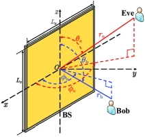
Figure 2: Illustration for a planar CAPA.

III-C1 Planar CAPA

We consider that the BS employs a planar CAPA situated on the $x$-$z$ plane and centered at the origin, as depicted in Fig. 2. The edges of $\mathcal{A}$ are parallel to the coordinate axes, with physical dimensions $L_{x}$ and $L_{z}$ along the $x$- and $z$-axes, respectively. It follows that

$${\mathcal{A}}=\{(x,0,z)|x,z\in\left[-{L_{x}}/{2},{L_{z}}/{2}\right]\},$$ (52)

with the size $\lvert\mathcal{A}\rvert=L_{x}L_{z}$. For each user $k\in\{\rm{b},\rm{e}\}$, let $r_{k}$ denote the distance from the center of $\mathcal{A}$ to the center of $\mathcal{A}_{\mathsf{k}}$, and let $\phi_{k}\in[0,\pi]$ and $\theta_{k}\in[0,\pi]$ represent the corresponding azimuth and elevation angles, respectively. Accordingly, $\mathcal{A}_{\mathsf{k}}$ is centered at ${\mathbf{r}}_{k}=[r_{k}\Phi_{k},r_{k}\Psi_{k},r_{k}\Theta_{k}]^{\mathsf{T}}$, where $\Phi_{k}\triangleq\cos{\phi_{k}}\sin{\theta_{k}}$, $\Psi_{k}\triangleq\sin{\phi_{k}}\sin{\theta_{k}}$, and $\Theta_{k}\triangleq\cos{\theta_{k}}$. Consequently, for $\mathbf{s}=[x,0,z]^{\mathsf{T}}\in\mathcal{A}$, by inserting $\mathbf{e}=[0,1,0]^{\mathsf{T}}$ and $\left\|\mathbf{r}_{k}-\mathbf{s}\right\|=(x^{2}+z^{2}-2r_{k}\left(\Phi_{k}x+\Theta_{k}z\right)+r_{k}^{2})^{\frac{1}{2}}$ into (51), we derive the channel response for user $k$ as follows:

$$\begin{split}h_{k}\left(\mathbf{s}\right)&=\frac{\mathrm{j}k_{0}\eta\sqrt{r_{k}\Psi_{k}}\mathrm{e}^{-\mathrm{j}k_{0}(x^{2}+z^{2}-2r_{k}\left(\Phi_{k}x+\Theta_{k}z\right)+r_{k}^{2})^{\frac{1}{2}}}}{\sqrt{4\pi}(x^{2}+z^{2}-2r_{k}\left(\Phi_{k}x+\Theta_{k}z\right)+r_{k}^{2})^{\frac{3}{4}}}\\ &\triangleq h_{k}(x,z).\end{split}$$ (53)

To characterize the MSR, we firstly derive the channel gain for each user and the channel correlation factor as follows.

Lemma 6.

With the planar CAPA, the channel gain for user $k\in\{{\mathrm{b},\mathrm{e}}\}$ can be expressed as follows:

$$g_{k}^{\mathrm{c}}=\frac{k_{0}^{2}\eta^{2}}{4\pi}\sum_{x\in\mathcal{X}_{k}}{\sum_{z\in\mathcal{Z}_{k}}{\arctan}}\bigg{(}\frac{xz}{\Psi_{k}\sqrt{\Psi_{k}^{2}+x^{2}+z^{2}}}\bigg{)},$$ (54)

where ${\mathcal{X}}_{k}\triangleq\{\frac{L_{x}}{2r_{k}}\pm\Phi_{k}\}$, and ${\mathcal{Z}}_{k}\triangleq\{\frac{L_{z}}{2r_{k}}\pm\Theta_{k}\}$. Additionally, the channel correlation factor can be approximated as follows:

$$\begin{split}\rho_{\mathrm{c}}=&\frac{\pi^{2}\left|\mathcal{A}\right|}{4T^{2}}\sum\nolimits_{t=1}^{T}{\sum\nolimits_{t^{\prime}=1}^{T}{\sqrt{\left(1-\psi_{t}^{2}\right)\left(1-\psi_{t^{\prime}}^{2}\right)}}}\\ &\times h_{\mathrm{b}}^{*}({L_{x}\psi_{t}}/{2},{L_{z}\psi_{t^{\prime}}}/{2})h_{\mathrm{e}}({L_{x}\psi_{t}}/{2},{L_{z}\psi_{t^{\prime}}}/{2}),\end{split}$$ (55)

where $T$ is a complexity-vs-accuracy tradeoff parameter, and $\psi_{t}=\cos\left(\frac{\left(2t-1\right)\pi}{2n}\right)$.

Proof:

Please refer to Appendix -G for more details. ∎

Given that the MSR in (36) is expressed as a function of the channel gain of each user and the channel correlation factor, after deriving $g_{k}^{\mathrm{c}}$ and $\rho_{\mathrm{c}}$, we can obtain the MSR achieved by the planar CAPA as $\mathcal{R}_{\mathrm{c}}=R\left(g_{\mathrm{b}}^{\mathrm{c}},g_{\mathrm{e}}^{\mathrm{c}},\overline{\rho}_{\mathrm{c}}\right)$, where $\overline{\rho}_{\mathrm{c}}=\frac{\left|\rho_{\mathrm{c}}\right|^{2}}{g_{\mathrm{b}}^{\mathrm{c}}g_{\mathrm{e}}^{\mathrm{c}}}$.

To further elucidate the properties of planar CAPAs in the secure transmission, we analyze the asymptotic MSR where $\mathcal{A}$ becomes infinitely large, i.e., $L_{x},L_{z}\rightarrow\infty$. Under this condition, the channel gain for user $k\in\{{\mathrm{b},\mathrm{e}}\}$ satisfies

$$\lim_{L_{x},L_{z}\rightarrow\infty}g_{k}^{\mathrm{c}}=\frac{k_{0}^{2}\eta^{2}}{4\pi}\frac{4\pi}{2}=\frac{k_{0}^{2}\eta^{2}}{2},$$ (56)

which is a constant value. Additionally, while $\lim_{L_{x},L_{z}\rightarrow\infty}\overline{\rho}_{\mathrm{c}}$ is computationally intractable, the numerical results shown in [33, 34] indicate that this limit is much less than one, i.e., $1-\lim_{L_{x},L_{z}\rightarrow\infty}\overline{\rho}_{\mathrm{c}}\approx 1$. Based on these findings, we can determine the asymptotic MSR as follows.

Corollary 1.

When $L_{x},L_{z}\rightarrow\infty$, the asymptotic MSR for the planar CAPA is given by

$$\lim_{L_{x},L_{z}\rightarrow\infty}\mathcal{R}_{\mathrm{c}}\approx\log_{2}\left(1+\frac{\overline{\gamma}_{\mathrm{b}}k_{0}^{2}\eta^{2}}{2}\right).$$ (57)

Proof:

The results are obtained by substituting $1-\overline{\rho}\approx 1$ and the results in (56) into (36). ∎

Remark 4.

For the infinitely large planar CAPA, the received power at Bob is maximized by the MRT source current, i.e., $j_{\mathsf{msr}}\left(\mathbf{s}\right)=j_{\mathsf{mrt}}\left(\mathbf{s}\right)$, while Eve’s received power is minimized to zero, reaching the upper limit of secrecy performance.

Remark 5.

The MSR will converge to an upper bound rather than increasing indefinitely with the aperture size, a observation that is intuitively reasonable from the standpoint of energy conservation.

III-C2 Planar SPDA

For comparison, we next examine a case where the above planar CAPA is partitioned into $M=M_{z}M_{x}$ spatially discrete elements. Here, $M_{x}=2\tilde{M}_{x}+1$ and $M_{z}=2\tilde{M}_{z}+1$ represent the number of antenna elements along the $x$- and $z$-axes respectively, as illustrated in Fig. 3. The size of each element is denoted by $\sqrt{{A}_{\mathrm{s}}}\times\sqrt{{A}_{\mathrm{s}}}$, and the inter-element distance is $d$, where $\sqrt{{A}_{\mathrm{s}}}\leq d\ll r_{k}$. Under this configuration, the central location of each element is $[m_{x}d,0,m_{z}d]^{\mathsf{T}}$, where $m_{x}\in\mathcal{M}_{x}\triangleq\{0,\pm 1,\ldots,\pm\tilde{M}_{x}\}$ and $m_{z}\in\mathcal{M}_{z}\triangleq\{0,\pm 1,\ldots,\pm\tilde{M}_{z}\}$. Additionally, we have $L_{x}\approx M_{x}d$, $L_{z}\approx M_{z}d$, and

$$\mathcal{A}=\left\{(m_{x}d+\ell_{x},0,m_{z}d+\ell_{z})\left|\begin{array}[]{c}\ell_{x},\ell_{z}\in[-\frac{\sqrt{A_{\mathrm{s}}}}{2},\frac{\sqrt{A_{\mathrm{s}}}}{2}],\\ m_{x}\in\mathcal{M}_{x},m_{z}\in\mathcal{M}_{z}\\ \end{array}\right.\right\}.$$ (58)

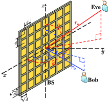
Figure 3: Illustration for Planar SPDA.

For the planar SPDA, given that the size of each element is much smaller than the distance between the BS and the user, i.e.,$\sqrt{{A}_{\mathrm{s}}}\ll r_{k}$, the variation in the channel across an element is negligible. Consequently, we can express the channel gain and correlation factor as follows:

$$g_{k}^{\mathrm{s}} =A_{\mathrm{s}}\sum_{m_{x}\in\mathcal{M}_{x}}{\sum_{m_{z}\in\mathcal{M}_{z}}{\left|h_{k}(m_{x}d,m_{z}d)\right|}^{2}},$$ (59)

$$\rho_{\mathrm{s}} =A_{\mathrm{s}}\sum_{m_{x}\in\mathcal{M}_{x}}{\sum_{m_{z}\in\mathcal{M}_{z}}{h_{\mathrm{b}}^{*}(m_{x}d,m_{z}d)h_{\mathrm{e}}(m_{x}d,m_{z}d)}}.$$ (60)

Notably, the channel gain $g_{k}^{\mathrm{s}}$ can be calculated as follow.

Lemma 7.

With the planar SPDA, the channel gain for user $k\in{\mathrm{b},\mathrm{e}}$ is given by

$$g_{k}^{\mathrm{s}}=\!\frac{A_{\mathrm{s}}k_{0}^{2}\eta^{2}}{4\pi d^{2}}\!\sum_{x\in\mathcal{X}_{k}}{\sum_{z\in\mathcal{Z}_{k}}\!{\arctan}}\bigg{(}\frac{xz}{\Psi_{k}\sqrt{\Psi_{k}^{2}\!+\!x^{2}\!+\!z^{2}}}\bigg{)}\!=\zeta_{\mathrm{oc}}g_{k}^{\mathrm{c}},$$ (61)

where $\zeta_{\mathrm{oc}}\triangleq\frac{A_{\mathrm{s}}}{d^{2}}$ represents the array occupation ratio (AOR).

Proof:

Please refer to Appendix -H for more details. ∎

Remark 6.

It can be observed from (61) that the channel gain for each user achieved by the SPDA converges to that of the CAPA when $\zeta_{\mathrm{oc}}=1$. This result is intuitive, as an SPDA effectively becomes a CAPA when the AOR equals $1$.

Having derive the MSR for the SPDA, viz., $\mathcal{R}_{\mathrm{s}}=R\left(g_{\mathrm{b}}^{\mathrm{s}},g_{\mathrm{e}}^{\mathrm{s}},\overline{\rho}_{\mathrm{s}}\right)$ with $\overline{\rho}_{\mathrm{s}}=\frac{\left|\rho_{\mathrm{s}}\right|^{2}}{g_{\mathrm{b}}^{\mathrm{s}}g_{\mathrm{e}}^{\mathrm{s}}}$, we can then obtain its asymptotic expression by following the steps similar to the derivations for the planar CAPA. In particular, as the number of antenna element $M_{x},M_{z}$ grows, the MSR achieved by the SPDA approaches to the following upper bound:

$$\lim_{M_{x},M_{z}\rightarrow\infty}\mathcal{R}_{\mathrm{s}}\approx\log_{2}\left(1+\frac{\overline{\gamma}_{\mathrm{b}}k_{0}^{2}\eta^{2}\zeta_{\mathrm{oc}}}{2}\right).$$ (62)

IV Analysis of the Minimum Required Power

In this section, we will analyze the MRP.

IV-A Problem Reformulation

The problem in (8b) can be rewritten as follows:

$$\min_{{p},\kappa(\mathbf{s})}~~ ~p$$ (63a)

$${\rm{s.t.}}~~~ \frac{1+p\left|\mathcal{A}_{\mathrm{b}}\right|\sigma_{\mathrm{b}}^{-2}\left|\int_{\mathcal{A}}{h_{\mathrm{b}}}(\mathbf{s})\kappa(\mathbf{s})\mathrm{d}\mathbf{s}\right|^{2}}{1+p\left|\mathcal{A}_{\mathrm{e}}\right|\sigma_{\mathrm{e}}^{-2}\left|\int_{\mathcal{A}}{h_{\mathrm{e}}}(\mathbf{s})\kappa(\mathbf{s})\mathrm{d}\mathbf{s}\right|^{2}}\geq 2^{\mathsf{R}_{0}},$$ (63b)

$$p>0,~\int_{\mathcal{A}}{\left|\kappa(\mathbf{s})\right|^{2}\mathrm{d}\mathbf{s}}=1,$$ (63c)

where $\int_{\mathcal{A}}{\left|j(\mathbf{s})\right|^{2}\mathrm{d}\mathbf{s}}=p$ and $\kappa(\mathbf{s})=\frac{j(\mathbf{s})}{\sqrt{p}}$. After multiplying both sides of (63b) by $1+p\left|\mathcal{A}_{\mathrm{e}}\right|\sigma_{\mathrm{e}}^{-2}\left|\int_{\mathcal{A}}{h_{\mathrm{e}}}(\mathbf{s})\kappa(\mathbf{s})\mathrm{d}\mathbf{s}\right|^{2}$ and performing some basic manipulations, we obtain

$$\int_{\mathcal{A}}{\int_{\mathcal{A}}{}p\kappa^{*}(\mathbf{s})D\left(\mathbf{s},\mathbf{s}^{\prime}\right)\kappa(\mathbf{s}^{\prime})\mathrm{d}\mathbf{s}}\mathrm{d}\mathbf{s}^{\prime}\geq 2^{\mathsf{R}_{0}}-1,$$ (64)

where

$$D\left(\mathbf{s},\mathbf{s}^{\prime}\right)=\frac{\left|\mathcal{A}_{\mathrm{b}}\right|}{\sigma_{\mathrm{b}}^{2}}h_{\mathrm{b}}(\mathbf{s})h_{\mathrm{b}}^{*}(\mathbf{s}^{\prime})-2^{\mathsf{R}_{0}}\frac{\left|\mathcal{A}_{\mathrm{e}}\right|}{\sigma_{\mathrm{e}}^{2}}h_{\mathrm{e}}(\mathbf{s})h_{\mathrm{e}}^{*}(\mathbf{s}^{\prime}).$$ (65)

Furthermore, we have

$$\int_{\mathcal{A}}{\int_{\mathcal{A}}{}p\kappa^{*}(\mathbf{s})D\left(\mathbf{s},\mathbf{s}^{\prime}\right)\kappa(\mathbf{s}^{\prime})\mathrm{d}\mathbf{s}}\mathrm{d}\mathbf{s}^{\prime}\leq p\lambda_{D}^{\max},$$ (66)

where $\lambda_{D}^{\max}$ denotes the principal eigenvalue of operator $D\left(\mathbf{s},\mathbf{s}^{\prime}\right)$. By combining (65) with (66), it follows that $p\geq\frac{2^{\mathsf{R}_{0}}-1}{\lambda_{D}^{\max}}>0$. This implies that the minimum value of $p$, i.e., the MRP, can be expressed as follows:

$$\mathcal{P}_{\star}=\frac{2^{\mathsf{R}_{0}}-1}{\lambda_{D}^{\max}}.$$ (67)

In this case, we have

$$\int_{\mathcal{A}}{\int_{\mathcal{A}}\kappa^{*}(\mathbf{s})D\left(\mathbf{s},\mathbf{s}^{\prime}\right)\kappa(\mathbf{s}^{\prime})\mathrm{d}\mathbf{s}}\mathrm{d}\mathbf{s}^{\prime}=\lambda_{D}^{\max},$$ (68)

which indicates that the associate $\kappa(\mathbf{s})$ aligns with the normalized principal eigenfunction of $D\left(\mathbf{s},\mathbf{s}^{\prime}\right)$.

IV-B Minimum Required Power & Optimal Current Distribution

The above arguments imply that the MRP and the associate current distribution correspond to the principal eigenvalue and eigenfunction of $D\left(\mathbf{s},\mathbf{s}^{\prime}\right)$, respectively. Their closed-form expressions are given as follows.

Theorem 5.

The MRP for CAPA-based secure transmission to guarantee a target secrecy rate $\mathsf{R}_{0}$ can be expressed as follows:

$$\mathcal{P}_{\star}=\frac{2\left(2^{\mathsf{R}_{0}}-1\right)}{\alpha+\sqrt{\alpha^{2}+\beta}},$$ (69)

where $\alpha=\left|\mathcal{A}_{\mathrm{b}}\right|\sigma_{\mathrm{b}}^{-2}g_{\mathrm{b}}-2^{\mathsf{R}_{0}}\left|\mathcal{A}_{\mathrm{e}}\right|\sigma_{\mathrm{e}}^{-2}g_{\mathrm{e}}$, and $\beta=2^{\mathsf{R}_{0}+2}\left|\mathcal{A}_{\mathrm{b}}\right|\left|\mathcal{A}_{\mathrm{e}}\right|\sigma_{\mathrm{b}}^{-2}\sigma_{\mathrm{e}}^{-2}g_{\mathrm{b}}g_{\mathrm{e}}\left(1-\overline{\rho}\right)$. The optimal current distribution is given by

$$\begin{split}j_{\mathsf{mrp}}\left(\mathbf{s}\right)=\sqrt{\mathcal{P}_{\star}}\frac{h^{*}_{\mathrm{b}}(\mathbf{s})-\tau h^{*}_{\mathrm{e}}(\mathbf{s})}{\sqrt{\int_{\mathcal{A}}\left\lvert h^{*}_{\mathrm{b}}(\mathbf{s})-\tau h^{*}_{\mathrm{e}}(\mathbf{s})\right\rvert^{2}{\rm{d}}{\mathbf{s}}}},\end{split}$$ (70)

where $\tau=\frac{{\left|\mathcal{A}_{\mathrm{b}}\right|g_{\mathrm{b}}}{\sigma_{\mathrm{b}}^{-2}}+{\left|\mathcal{A}_{\mathrm{e}}\right|g_{\mathrm{e}}2^{\mathsf{R}_{0}}}{\sigma_{\mathrm{e}}^{-2}}-\sqrt{\alpha^{2}+\beta}}{2\left|\mathcal{A}_{\mathrm{b}}\right|\sigma_{\mathrm{b}}^{-2}\rho}$.

Proof:

The proof is similar to that of Lemma 4. ∎

Remark 7.

The MRP given in (69) is determined by the channel gain for each user and the channel correlation factor. This expression is applicable to any aperture, regardless of its location, shape, and size.

We next compare the MRP with the required power achieved by ZF and MRT beamforming. When MRT beamforming is utilized, we have $j({\mathbf{s}})=\sqrt{p}\frac{h^{*}_{\mathrm{b}}(\mathbf{s})}{{\sqrt{\int_{\mathcal{A}}\left\lvert h^{*}_{\mathrm{b}}(\mathbf{s})\right\rvert^{2}{\rm{d}}{\mathbf{s}}}}}$ (as per (43)), and the minimum required transmission power to guarantee a secrecy transmission rate of $\mathsf{R}_{0}$ is given by

$$\mathcal{P}_{\mathsf{mrt}}=\frac{2^{\mathsf{R}_{0}}-1}{\left|\mathcal{A}_{\mathrm{b}}\right|\sigma_{\mathrm{b}}^{-2}g_{\mathrm{b}}-2^{\mathsf{R}_{0}}\left|\mathcal{A}_{\mathrm{e}}\right|\sigma_{\mathrm{e}}^{-2}g_{\mathrm{e}}\overline{\rho}}.$$ (71)

By noting that fact that $\overline{\rho}\in[0,1]$, we can prove that

$$\frac{\mathcal{P}_{\mathsf{mrt}}}{\mathcal{P}_{\star}}=\frac{1}{2}\frac{\alpha+\sqrt{\alpha^{2}+\beta}}{\left|\mathcal{A}_{\mathrm{b}}\right|\sigma_{\mathrm{b}}^{-2}g_{\mathrm{b}}-2^{\mathsf{R}_{0}}\left|\mathcal{A}_{\mathrm{e}}\right|\sigma_{\mathrm{e}}^{-2}g_{\mathrm{e}}\overline{\rho}}>1.$$ (72)

Furthermore, we have the following observations.

Remark 8.

It is observed that the proposed optimal current distribution outperforms MRT beamforming in terms of minimizing the transmit power. Besides, the optimal current distribution $j_{\mathsf{mrp}}\left(\mathbf{s}\right)$ can achieve an arbitrary large target secrecy rate as long as the transmission power is sufficiently high. In contrast, the MRT cannot achieve a secrecy rate greater than $\log_{2}\left(\left|\mathcal{A}_{\mathrm{b}}\right|\sigma_{\mathrm{b}}^{-2}g_{\mathrm{b}}\right)-\log_{2}\left(\left|\mathcal{A}_{\mathrm{e}}\right|\sigma_{\mathrm{e}}^{-2}g_{\mathrm{e}}\overline{\rho}\right)$, regardless of the transmission power level.

We then consider ZF beamforming, which yields $\sqrt{p}\frac{h^{*}_{\mathrm{b}}(\mathbf{s})-\frac{g_{\mathrm{b}}}{\rho}\overline{\rho}h^{*}_{\mathrm{e}}(\mathbf{s})}{\sqrt{\int_{\mathcal{A}}\left\lvert h^{*}_{\mathrm{b}}(\mathbf{s})-\frac{g_{\mathrm{b}}}{\rho}\overline{\rho}h^{*}_{\mathrm{e}}(\mathbf{s})\right\rvert^{2}{\rm{d}}{\mathbf{s}}}}$ (as per (47)), and the minimum required transmission power to guarantee a secrecy transmission rate of $\mathsf{R}_{0}$ is given by

$$\mathcal{P}_{\mathsf{zf}}=\frac{2^{\mathsf{R}_{0}}}{\left|\mathcal{A}_{\mathrm{b}}\right|\sigma_{\mathrm{b}}^{-2}g_{\mathrm{b}}\left(1-\overline{\rho}\right)}.$$ (73)

By letting ${\mathsf{R}_{0}}\rightarrow\infty$, we have

$$\begin{split}\lim_{{\mathsf{R}_{0}}\rightarrow\infty}\frac{1}{\alpha+\sqrt{\alpha^{2}+\beta}}&=\lim_{{\mathsf{R}_{0}}\rightarrow\infty}\frac{\sqrt{\alpha^{2}+\beta}-\alpha}{\beta}\\ &=\frac{1}{2\left|\mathcal{A}_{\mathrm{b}}\right|\sigma_{\mathrm{b}}^{-2}g_{\mathrm{b}}\left(1-\overline{\rho}\right)},\end{split}$$ (74)

which suggests that

$$\lim_{{\mathsf{R}_{0}}\rightarrow\infty}\mathcal{P}_{\star}\simeq\frac{2^{\mathsf{R}_{0}}}{\left|\mathcal{A}_{\mathrm{b}}\right|\sigma_{\mathrm{b}}^{-2}g_{\mathrm{b}}\left(1-\overline{\rho}\right)}=\mathcal{P}_{\mathsf{zf}}.$$ (75)

Remark 9.

The results in (75) suggest that ZF beamforming is asymptotically optimal when achieving an infinitely large secrecy rate target.

IV-C Typical Cases

Since the MRP is expressed as a function of the channel gains and the channel correlation factor, the MRP for both the planar CAPA and SPDA under the LoS channel can be readily obtained based on the results in Lemma 6 and 7, respectively. Therefore, in this subsection, we will focus on the asymptotic behaviors of $\mathcal{P}$ as $L_{x},L_{z}\rightarrow\infty$ or $M_{x},M_{z}\rightarrow\infty$ to gain further insights, where the considered channel model and array structure are the same as those detailed in Section III-C.

IV-C1 Planar CAPA

The asymptotic MRP for the planar CAPA with infinitely large aperture is given as follows.

Corollary 2.

When $L_{x},L_{z}\rightarrow\infty$, the MRP satisfies

$$\lim_{L_{x},L_{z}\rightarrow\infty}\mathcal{P}_{\star}\approx\frac{2\left(2^{\mathsf{R}_{0}}-1\right)}{k_{0}^{2}\eta^{2}\left|\mathcal{A}_{\mathrm{b}}\right|\sigma_{\mathrm{b}}^{-2}}.$$ (76)

Proof:

Similar to the proof of Corollary 1. ∎

Remark 10.

The results of Corollary 2 suggest that as the aperture size increases, the MRP for the planar CAPA will converge to an lower bound that is larger than zero.

IV-C2 Planar SPDA

In the case of the planar SPDA, when the antenna number grows to infinity, i.e., $M_{x},M_{z}\rightarrow\infty$, the MRP approaches to the follow lower bound:

$$\lim_{M_{x},M_{z}\rightarrow\infty}\mathcal{P}_{\star}\approx\frac{2\left(2^{\mathsf{R}_{0}}-1\right)}{k_{0}^{2}\eta^{2}\left|\mathcal{A}_{\mathrm{b}}\right|\sigma_{\mathrm{b}}^{-2}\zeta_{\mathrm{oc}}}.$$ (77)

We note that for extremely large arrays, the minimum transmit power required by an SPDA for a given target secrecy rate reduces to that of the CAPA when $\zeta_{\mathrm{oc}}=1$.

V Numerical Results

In this section, numerical results are presented to demonstrate the secrecy performance achieved by CAPAs. For clarity, the simulations employ the planar arrays specified in Section III-C. Without otherwise specification, the simulation parameters are set as follows: $\lambda=0.125$ m, $\left|\mathcal{A}_{\mathrm{b}}\right|=\left|\mathcal{A}_{\mathrm{e}}\right|=\frac{\lambda^{2}}{4\pi}$, $\frac{P}{\sigma^{2}_{\mathrm{b}}}=\frac{P}{\sigma^{2}_{\mathrm{e}}}=10$ dB, $L_{x}=L_{z}$, $(r_{\mathrm{b}},\theta_{\mathrm{b}},\phi_{\mathrm{b}})=(10\,\rm{m},\frac{\pi}{6},\frac{\pi}{6})$, $(r_{\mathrm{e}},\theta_{\mathrm{e}},\phi_{\mathrm{e}})=(20\,\rm{m},\frac{\pi}{3},\frac{\pi}{3})$, and $T=100$.

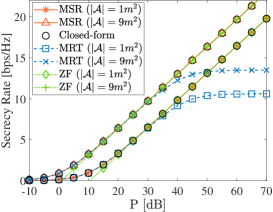
Figure 4: Secrecy rates versus power budget $P$.

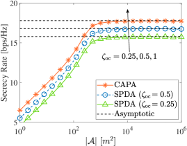
Figure 5: MSRs versus aperture size $\left|\mathcal{A}\right|$.

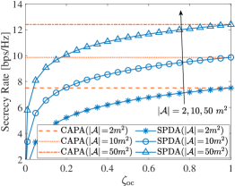
Figure 6: MSRs versus AOR $\zeta_{\mathrm{oc}}$.

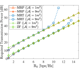
Figure 7: Required powers versus target secrecy rate $\mathsf{R}_{0}$.

V-A Maximum Secrecy Rate

Figure 4 illustrates the secrecy rate achieved by the CAPA with different aperture sizes as a function of the power budget. As observed, the derived closed-form expressions closely align with the simulation results, which validates the correctness of our previously derived results. For comparison, the secrecy rates achieved by MRT and ZF beamforming schemes are also presented. The results show that the proposed optimal current distribution yields better secrecy rate than both the MRT and ZF-based schemes. Moreover, as the transmit power increases, the secrecy rate achieved by MRT beamforming converges to a finite constant, while the rates achieved by ZF beamforming and the optimal current distribution increase monotonically. This demonstrates that the high-SNR slope for the MSR is greater than that achieved by MRT beamforming.

From Figure 4, it can be also observed that in the low-SNR regime, the secrecy rate achieved by MRT beamforming is nearly identical to that achieved by the optimal current distribution. This is because, at low SNRs, Gaussian noise dominates over information leakage, making MRC beamforming more effective for enhancing the secrecy rate. In contrast, at high SNRs, the secrecy rate achieved by ZF beamforming closely approaches that of the optimal current distribution. This is because, in the high-SNR regime, information leakage becomes the dominant factor over Gaussian noise, making leakage cancellation essential for improving the secrecy rate. These observations align with the discussions in Section III-B3.

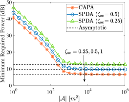
Figure 8: MRPs versus aperture size $\left|\mathcal{A}\right|$.

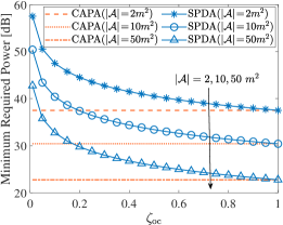
Figure 9: MRPs versus AOR $\zeta_{\mathrm{oc}}$.

To further investigate the behavior of the MSR as the BS aperture size increases, we present the MSR as a function of $\left|\mathcal{A}\right|$ for both CAPA and SPDA in Figure 5. It can be observed that as the aperture size grows, the MSRs increase and eventually approach their upper bounds, as indicated in (57) and (62), which adheres to the principle of energy conservation. This observation verifies our discussions in Remark 5. Additionally, the results in Figure 5 demonstrate that for the same aperture size, CAPA achieves superior secrecy performance compared to conventional SPDA. To further highlight the performance gap between CAPA and SPDA in terms of achievable MSR, we plot the MSR for SPDAs against the AOR in Figure 6. This graph illustrates the MSR for an SPDA gradually converges with that of a CAPA as the AOR approaches one, which corroborates the statements in Remark 6.

V-B Minimum Required Power

Figure 7 illustrates the MRP and the transmission power needed for ZF and MRT beamforming to achieve different target secrecy rates ${\mathsf{R}}_{0}$. It can be observed that while the required powers for MRT beamforming are nearly identical to the MRP for small values of $\mathsf{R}_{0}$, the gap becomes significant as $\mathsf{R}_{0}$ grows, with MRT requiring substantially more power than the MRP. Notably, when the target secrecy rate exceeds a certain threshold, MRT beamforming becomes incapable of achieving it, regardless of the available transmission power. In contrast, the current distribution designed to achieve the MRP can support arbitrarily high secrecy rates, provided sufficient transmission power is available. These findings align with the discussions in Remark 8. Furthermore, we observe that when achieving a high target secrecy rate, ZF beamforming yields performance virtually identical to that of the optimal current distribution, which corroborates the results discussed in Remark 9. The above observations highlight the superiority of the proposed optimal current design in terms of minimizing transmit power while guaranteeing a target secrecy rate.

In Figure 8, we present the MRP as a function of the BS aperture size $\left|\mathcal{A}\right|$. Initially, the MRP decreases as $\left|\mathcal{A}\right|$ increases, which indicates that using a larger aperture can increase the power utilization efficiency. However, as the aperture size continues to grow, the MRP converges to a non-zero lower bound. This observation is consistent with Remark 10 and aligns with the physical limitation that the required transmission power cannot be reduced to zero, even with an extremely large array size. Additionally, Figure 9 shows the MRP for both CAPAs and SPDAs as a function of the AOR. Similar to the MSR, the MRP for an SPDA gradually converges to that of a CAPA as the AOR approaches $1$.

VI Conclusion

This article has developed a novel secure transmission framework using CAPAs and analyzed its fundamental secrecy performance limits. We derived closed-form expressions for the MSR under a power constraint and the MRP to achieve a target secrecy rate, along with the corresponding optimal continuous current distributions. We proved that the rate-optimal source current simplifies to MRT beamforming in the low-SNR region and to ZF beamforming in the high-SNR region. Additionally, we showed that the power-optimal current converges to ZF beamforming in the high-SNR regime. Through both theoretical analyses and numerical simulations, we demonstrated that CAPAs provide superior secrecy performance compared to conventional SPDAs. These findings underscore the potential of CAPAs as a promising paradigm for secure wireless communication.

-A Proof of Lemma 1

Inserting (13) and (14) into the left-hand side of (15) gives

$$\int_{\mathcal{A}}Q\left(\mathbf{s},\mathbf{s}_{1}\right)\hat{Q}\left(\mathbf{s}_{1},\mathbf{s}^{\prime}\right){\rm{d}}\mathbf{s}_{1}=\int_{\mathcal{A}}\left(\delta(\mathbf{s}-\mathbf{s}_{1})+\mu h_{\mathrm{e}}(\mathbf{s})h_{\mathrm{e}}^{*}(\mathbf{s}_{1})\right)$$

$$\times\left(\delta(\mathbf{s}_{1}-\mathbf{s}^{\prime})-\frac{\mu h_{\mathrm{e}}(\mathbf{s}_{1})h_{\mathrm{e}}^{*}(\mathbf{s}^{\prime})}{1+\mu g_{\mathrm{e}}}\right)\mathrm{d}\mathbf{s}_{1}=\delta(\mathbf{s}-\mathbf{s}^{\prime})$$

$$+\left(\mu-\frac{\mu+\mu^{2}g_{\mathrm{e}}}{1+\mu g_{\mathrm{e}}}\right)h_{\mathrm{e}}(\mathbf{s})h_{\mathrm{e}}^{*}(\mathbf{s}^{\prime})=\delta(\mathbf{s}-\mathbf{s}^{\prime}).$$ (A1)

Following the same approach to obtain (-A), we also obtain

$$\int_{\mathcal{A}}\hat{Q}\left(\mathbf{s},\mathbf{s}_{1}\right)Q\left(\mathbf{s}_{1},\mathbf{s}^{\prime}\right){\rm{d}}\mathbf{s}_{1}=\delta(\mathbf{s}-\mathbf{s}^{\prime}).$$ (A2)

This completes the proof of Lemma 1.

-B Proof of Lemma 2

Inserting (13) and (14) into the left-hand side of (16) gives

$$E(\mathbf{s}_{1},\mathbf{s}_{1}^{\prime})= \int_{\mathcal{A}}{\int_{\mathcal{A}}}(\delta(\mathbf{s}_{1}-\mathbf{s})+\mu h_{\mathrm{e}}(\mathbf{s}_{1})h_{\mathrm{e}}^{*}(\mathbf{s}))A_{\rm{e}}(\mathbf{s},\mathbf{s}^{\prime})$$

$$\times(\delta(\mathbf{s}^{\prime}-\mathbf{s}_{1}^{\prime})+\mu h_{\mathrm{e}}(\mathbf{s}^{\prime})h_{\mathrm{e}}^{*}(\mathbf{s}_{1}^{\prime}))\mathrm{d}\mathbf{s}\mathrm{d}\mathbf{s}^{\prime}.$$ (A3)

We then calculate $E(\mathbf{s}_{1},\mathbf{s}^{\prime}_{1})$ as follows. According to that fact of $\int_{{\mathcal{A}}}\delta({\mathbf{x}}-{\mathbf{x}}_{0})f(\mathbf{x}){\rm{d}}{\mathbf{x}}=f({\mathbf{x}}_{0})$, the integral in terms of ${{\mathbf{s}}}$ involved in (-B) can be calculated as follows:

$$\int_{\mathcal{A}}(\delta(\mathbf{s}_{1}-\mathbf{s})\!+\!\mu h_{\mathrm{e}}(\mathbf{s}_{1})h_{\mathrm{e}}^{*}(\mathbf{s}))(\delta(\mathbf{s}-\mathbf{s}^{\prime})\!+\!\overline{\gamma}_{\mathrm{e}}h_{\mathrm{e}}(\mathbf{s})h_{\mathrm{e}}^{*}(\mathbf{s}^{\prime}))\mathrm{d}\mathbf{s}$$

$$=\delta(\mathbf{s}_{1}-\mathbf{s}^{\prime})+(\mu+\overline{\gamma}_{\mathrm{e}}+\overline{\gamma}_{\mathrm{e}}\mu g_{\mathrm{e}})h_{\mathrm{e}}(\mathbf{s}_{1})h_{\mathrm{e}}^{*}(\mathbf{s}^{\prime}).$$ (A4)

We next calculate the integral in terms of ${{\mathbf{s}}}^{\prime}$, which yields

$$\int_{\mathcal{A}}\eqref{Denominator_Calculation_Forward_1}\times(\delta(\mathbf{s}^{\prime}-\mathbf{s}_{1}^{\prime})+\mu h_{\mathrm{e}}(\mathbf{s}^{\prime})h_{\mathrm{e}}^{*}(\mathbf{s}_{1}^{\prime}))\mathrm{d}\mathbf{s}^{\prime}$$

$$=\!\delta(\mathbf{s}_{1}\!-\!\mathbf{s}_{1}^{\prime})\!+\chi h_{\mathrm{e}}(\mathbf{s}_{1})h_{\mathrm{e}}^{*}(\mathbf{s}_{1}^{\prime}),$$ (A5)

where $\chi=\overline{\gamma}_{\mathrm{e}}\mu^{2}g_{\mathrm{e}}^{2}+\mu^{2}g_{\mathrm{e}}+2\overline{\gamma}_{\mathrm{e}}\mu g_{\mathrm{e}}+2\mu+\overline{\gamma}_{\mathrm{e}}$. Inserting $\mu=-\frac{1}{g_{\mathrm{e}}}\pm\frac{1}{g_{\mathrm{e}}\sqrt{1+\overline{\gamma}_{\mathrm{e}}g_{\mathrm{e}}}}$ into the expression of $\chi$, we can obtain $\chi=0$, which yields

$$E(\mathbf{s}_{1},\mathbf{s}^{\prime}_{1})=\delta(\mathbf{s}_{1}-\mathbf{s}_{1}^{\prime}),$$ (A6)

which completes the proof of Lemma 2.

-C Proof of Lemma 3

Equation (27) can be written as follows:

$$\begin{split}&\!C(\mathbf{s}_{2},\mathbf{s}_{2}^{\prime})\!=\!\underset{I_{1}}{\underbrace{\int_{\mathcal{A}}{\int_{\mathcal{A}}}\hat{Q}(\mathbf{s}_{2},\mathbf{s}_{1})B(\mathbf{s}_{1},\mathbf{s}_{1}^{\prime})\hat{Q}(\mathbf{s}_{1}^{\prime},\mathbf{s}_{2}^{\prime})\mathrm{d}\mathbf{s}_{1}\mathrm{d}\mathbf{s}_{1}^{\prime}}}\\ &~~~-\lambda_{B}\underset{I_{2}}{\underbrace{\int_{\mathcal{A}}{\int_{\mathcal{A}}{}}\hat{Q}(\mathbf{s}_{2},\mathbf{s}_{1})\delta(\mathbf{s}_{1}-\mathbf{s}_{1}^{\prime})\hat{Q}(\mathbf{s}_{1}^{\prime},\mathbf{s}_{2}^{\prime})\mathrm{d}\mathbf{s}_{1}\mathrm{d}\mathbf{s}_{1}^{\prime}}}.\end{split}$$ (A7)

Substituting (22) into $I_{1}$ gives

$$I_{1} =\int_{\mathcal{A}}{\int_{\mathcal{A}}{A_{\rm{b}}(\mathbf{s},\mathbf{s}^{\prime})}}\int_{\mathcal{A}}\hat{Q}(\mathbf{s}_{2},\mathbf{s}_{1})Q\left(\mathbf{s}_{1},\mathbf{s}\right)\mathrm{d}\mathbf{s}_{1}$$

$$\times\int_{\mathcal{A}}{Q\left(\mathbf{s}^{\prime},\mathbf{s}^{\prime}_{1}\right)\hat{Q}(\mathbf{s}_{1}^{\prime},\mathbf{s}_{2}^{\prime})}\mathrm{d}\mathbf{s}_{1}^{\prime}\mathrm{d}\mathbf{s}\mathrm{d}\mathbf{s}^{\prime}=\int_{\mathcal{A}}{\int_{\mathcal{A}}{A_{\rm{b}}(\mathbf{s},\mathbf{s}^{\prime})}}$$

$$\times\delta(\mathbf{s}_{2}-\mathbf{s})\delta(\mathbf{s}^{\prime}-\mathbf{s}_{2}^{\prime})\mathrm{d}\mathbf{s}\mathrm{d}\mathbf{s}^{\prime}=A_{\rm{b}}(\mathbf{s}_{2},\mathbf{s}_{2}^{\prime}).$$ (A8)

Moreover, $I_{2}$ can be calculated as follows:

$$I_{2} =\int_{\mathcal{A}}{\int_{\mathcal{A}}{}}\Big{(}\delta(\mathbf{s}_{2}-\mathbf{s}_{1})-\frac{\mu}{1+\mu g_{\mathrm{e}}}h_{\mathrm{e}}(\mathbf{s}_{2})h_{\mathrm{e}}^{*}(\mathbf{s}_{1})\Big{)}\delta(\mathbf{s}_{1}-\mathbf{s}_{1}^{\prime})$$

$$\times\Big{(}\delta(\mathbf{s}_{1}^{\prime}-\mathbf{s}_{2}^{\prime})-\frac{\mu}{1+\mu g_{\mathrm{e}}}h_{\mathrm{e}}(\mathbf{s}_{1}^{\prime})h_{\mathrm{e}}^{*}(\mathbf{s}_{2}^{\prime})\Big{)}\mathrm{d}\mathbf{s}_{1}\mathrm{d}\mathbf{s}_{1}^{\prime}$$

$$=\int_{\mathcal{A}}{}\Big{(}\delta(\mathbf{s}_{2}-\mathbf{s}_{1}^{\prime})-\frac{\mu}{1+\mu g_{\mathrm{e}}}h_{\mathrm{e}}(\mathbf{s}_{2})h_{\mathrm{e}}^{*}(\mathbf{s}_{1}^{\prime})\Big{)}$$

$$\times\Big{(}\delta(\mathbf{s}_{1}^{\prime}-\mathbf{s}_{2}^{\prime})-\frac{\mu}{1+\mu g_{\mathrm{e}}}h_{\mathrm{e}}(\mathbf{s}_{1}^{\prime})h_{\mathrm{e}}^{*}(\mathbf{s}_{2}^{\prime})\Big{)}\mathrm{d}\mathbf{s}_{1}^{\prime}$$

$$=\delta(\mathbf{s}_{2}-\mathbf{s}_{2}^{\prime})+\frac{\mu}{1+\mu g_{\mathrm{e}}}\left(\frac{\mu g_{\mathrm{e}}}{1+\mu g_{\mathrm{e}}}-2\right)h_{\mathrm{e}}(\mathbf{s}_{2})h_{\mathrm{e}}^{*}(\mathbf{s}_{2}^{\prime}).$$

Recalling that $\mu=-\frac{1}{g_{\mathrm{e}}}\pm\frac{1}{g_{\mathrm{e}}\sqrt{1+\overline{\gamma}_{\mathrm{e}}g_{\mathrm{e}}}}$ yields

$$\frac{\mu}{1+\mu g_{\mathrm{e}}}\left(\frac{\mu g_{\mathrm{e}}}{1+\mu g_{\mathrm{e}}}-2\right)=\frac{\mu(-2-\mu g_{\mathrm{e}})}{(1+\mu g_{\mathrm{e}})^{2}}=\overline{\gamma}_{\mathrm{e}},$$ (A9)

which leads to

$$I_{2}=\delta(\mathbf{s}_{2}-\mathbf{s}_{2}^{\prime})+\overline{\gamma}_{\mathrm{e}}h_{\mathrm{e}}(\mathbf{s}_{2})h_{\mathrm{e}}^{*}(\mathbf{s}_{2}^{\prime})=A_{\rm{e}}(\mathbf{s}_{2}-\mathbf{s}_{2}^{\prime}).$$ (A10)

By inserting (-C) and (A10) into (A7), the results of (28) follow immediately.

-D Proof of Lemma 4

Upon observing (28), the Hermitian operator $\breve{C}(\mathbf{s}_{2},\mathbf{s}_{2}^{\prime})\triangleq\overline{\gamma}_{\mathrm{b}}h_{\mathrm{b}}(\mathbf{s}_{2})h_{\mathrm{b}}^{*}(\mathbf{s}_{2}^{\prime})-\lambda_{B}\overline{\gamma}_{\mathrm{e}}h_{\mathrm{e}}(\mathbf{s}_{2})h_{\mathrm{e}}^{*}(\mathbf{s}_{2}^{\prime})$ is a function of $h_{\mathrm{b}}(\cdot)$ and $h_{\mathrm{e}}(\cdot)$. Therefore, it can be concluded that the eigenfunction of $\breve{C}(\mathbf{s}_{2},\mathbf{s}_{2}^{\prime})$ must lie in the subspace spanned by $h_{\mathrm{b}}(\cdot)$ and $h_{\mathrm{e}}(\cdot)$. This means that the eigenvalues and eigenfunctions of $\breve{C}(\mathbf{s}_{2},\mathbf{s}_{2}^{\prime})$ can be determined from the following equation:

$$\begin{split}&\int_{\mathcal{A}}\breve{C}(\mathbf{s}_{2},\mathbf{s}_{2}^{\prime})(ah^{*}_{\mathrm{b}}(\mathbf{s}_{2})-bh^{*}_{\mathrm{e}}(\mathbf{s}_{2}))\mathrm{d}\mathbf{s}_{2}\\ &=\xi(ah^{*}_{\mathrm{b}}(\mathbf{s}^{\prime}_{2})-bh^{*}_{\mathrm{e}}(\mathbf{s}^{\prime}_{2})),\end{split}$$ (A11)

where $\xi$ denotes the eigenvalue of $\breve{C}(\mathbf{s}_{2},\mathbf{s}_{2}^{\prime})$.

By performing some mathematical manipulations to the left-hand side of (A11), we can transform (A11) as follows:

$$\begin{split}&\left(a\overline{\gamma}_{\mathrm{b}}g_{\mathrm{b}}\!-\!b\overline{\gamma}_{\mathrm{b}}\rho\right)\!h^{*}_{\mathrm{b}}(\mathbf{s}^{\prime}_{2})\!-\!(a\lambda_{B}\overline{\gamma}_{\mathrm{e}}\rho^{*}\!-\!b\lambda_{B}\overline{\gamma}_{\mathrm{e}}g_{\mathrm{e}})h^{*}_{\mathrm{e}}(\mathbf{s}^{\prime}_{2})\\ &=a\xi h^{*}_{\mathrm{b}}(\mathbf{s}^{\prime}_{2})-b\xi h^{*}_{\mathrm{e}}(\mathbf{s}^{\prime}_{2}).\end{split}$$ (A12)

Based on (A12), we have

$$a\xi=a\overline{\gamma}_{\mathrm{b}}g_{\mathrm{b}}-b\overline{\gamma}_{\mathrm{b}}\rho,\ b\xi=a\lambda_{B}\overline{\gamma}_{\mathrm{e}}\rho^{*}-b\lambda_{B}\overline{\gamma}_{\mathrm{e}}g_{\mathrm{e}}.$$ (A13)

It follows that

$$\frac{\xi-\overline{\gamma}_{\mathrm{b}}g_{\mathrm{b}}}{\overline{\gamma}_{\mathrm{b}}\rho}=-\frac{b}{a},\quad\frac{\xi+\lambda_{B}\overline{\gamma}_{\mathrm{e}}g_{\mathrm{e}}}{\lambda_{B}\overline{\gamma}_{\mathrm{e}}\rho^{*}}=\frac{a}{b},$$ (A14)

which leads to the following equation with respect to $\xi$:

$$\frac{\xi-\overline{\gamma}_{\mathrm{b}}g_{\mathrm{b}}}{\overline{\gamma}_{\mathrm{b}}\rho}\frac{\xi+\lambda_{B}\overline{\gamma}_{\mathrm{e}}g_{\mathrm{e}}}{\lambda_{B}\overline{\gamma}_{\mathrm{e}}\rho^{*}}+1=0,$$ (A15)

or equivalently,

$$\xi^{2}-(\overline{\gamma}_{\mathrm{b}}g_{\mathrm{b}}-\lambda_{B}\overline{\gamma}_{\mathrm{e}}g_{\mathrm{e}})\xi-\lambda_{B}\overline{\gamma}_{\mathrm{b}}\overline{\gamma}_{\mathrm{e}}g_{\mathrm{b}}g_{\mathrm{e}}(1-\overline{\rho})=0.$$ (A16)

The solutions to the above equation are given by $\xi=\xi_{1}$ and $\xi=\xi_{2}$, where $\xi_{1}$ and $\xi_{2}$ are given in (33a) and (33b), respectively. In other words, $\xi=\xi_{1}$ and $\xi=\xi_{2}$ are the non-zero eigenvalues of $\breve{C}(\mathbf{s}_{2},\mathbf{s}_{2}^{\prime})$.

The above arguments imply that the eigen-decomposition of $\breve{C}(\mathbf{s}_{2},\mathbf{s}_{2}^{\prime})$ can be written as follows:

$$\breve{C}(\mathbf{s}_{2},\mathbf{s}_{2}^{\prime})=\sum\nolimits_{i=1}^{2}\xi_{i}\varphi_{i}(\mathbf{s}_{2})\varphi_{i}^{*}(\mathbf{s}_{2}^{\prime}),$$ (A17)

where $\{\varphi_{i}(\cdot)\}_{i=1}^{2}$ represents an orthonormal basis on ${\mathcal{A}}$. Furthermore, it holds that

$$\delta(\mathbf{s}_{2}-\mathbf{s}_{2}^{\prime})=\sum\nolimits_{i=1}^{\infty}\varphi_{i}(\mathbf{s}_{2})\varphi_{i}^{*}(\mathbf{s}_{2}^{\prime}),$$ (A18)

where $\{\varphi_{i}(\cdot)\}_{i=1}^{\infty}$ represents a complete orthonormal basis on ${\mathcal{A}}$. Taken together, we have

$$\begin{split}C(\mathbf{s}_{2},\mathbf{s}_{2}^{\prime})&=\breve{C}(\mathbf{s}_{2},\mathbf{s}_{2}^{\prime})+(1-\lambda_{B})\delta(\mathbf{s}_{2}-\mathbf{s}_{2}^{\prime})\\ &=\sum\nolimits_{i=1}^{2}(\xi_{i}+1-\lambda_{B})\varphi_{i}(\mathbf{s}_{2})\varphi_{i}^{*}(\mathbf{s}_{2}^{\prime})\\ &+\sum\nolimits_{i=3}^{\infty}(1-\lambda_{B})\varphi_{i}(\mathbf{s}_{2})\varphi_{i}^{*}(\mathbf{s}_{2}^{\prime}),\end{split}$$ (A19)

which represents the eigen-decomposition of $C(\mathbf{s}_{2},\mathbf{s}_{2}^{\prime})$. As a result, the eigenvalues of $C(\mathbf{s}_{2},\mathbf{s}_{2}^{\prime})$ are given by

$$\begin{split}&\lambda_{C,1}=\xi_{1}-\lambda_{B}+1,\ \lambda_{C,2}=\xi_{2}-\lambda_{B}+1,\\ &\lambda_{C,3}=\ldots=\lambda_{C,\infty}=-\lambda_{B}+1,\end{split}$$ (A20)

which completes the proof of Lemma 4.

-E Proof of Theorem 2

It follows from (34) that $\lambda_{B}=1$ or $\lambda_{B}=\xi_{1}+1$ or $\lambda_{B}=\xi_{2}+1$. For $\lambda_{B}=\xi_{1}+1$ or $\lambda_{B}=\xi_{2}+1$, we have

$$\lambda_{B}=\frac{\Delta\pm\sqrt{\Delta^{2}+4\lambda_{B}\overline{\gamma}_{\mathrm{b}}\overline{\gamma}_{\mathrm{e}}g_{\mathrm{b}}g_{\mathrm{e}}(1-\overline{\rho})}}{2}.$$ (A21)

This leads to

$$(2\lambda_{B}-\Delta)^{2}=\Delta^{2}+4\lambda_{B}\overline{\gamma}_{\mathrm{b}}\overline{\gamma}_{\mathrm{e}}g_{\mathrm{b}}g_{\mathrm{e}}(1-\overline{\rho}),$$ (A22)

which can be further simplified as follows:

$$\left(1+\overline{\gamma}_{\mathrm{e}}g_{\mathrm{e}}\right)(\lambda_{B}-1)^{2}-\Xi(\lambda_{B}-1)-\overline{\gamma}_{\mathrm{b}}\overline{\gamma}_{\mathrm{e}}g_{\mathrm{b}}g_{\mathrm{e}}(1-\overline{\rho})=0.$$

The solutions to the above equation are given by

$$\lambda_{B,1}=1+\frac{\Xi+\sqrt{\Xi^{2}+\Gamma}}{2\left(1+\overline{\gamma}_{\mathrm{e}}g_{\mathrm{e}}\right)},\ \lambda_{B,2}=1+\frac{\Xi-\sqrt{\Xi^{2}+\Gamma}}{2\left(1+\overline{\gamma}_{\mathrm{e}}g_{\mathrm{e}}\right)},$$

where $\Xi=\overline{\gamma}_{\mathrm{b}}g_{\mathrm{b}}-\overline{\gamma}_{\mathrm{e}}g_{\mathrm{e}}+\overline{\gamma}_{\mathrm{b}}\overline{\gamma}_{\mathrm{e}}g_{\mathrm{b}}g_{\mathrm{e}}(1-\overline{\rho})$, and $\Gamma=4\left(1+\overline{\gamma}_{\mathrm{e}}g_{\mathrm{e}}\right)\overline{\gamma}_{\mathrm{b}}\overline{\gamma}_{\mathrm{e}}g_{\mathrm{b}}g_{\mathrm{e}}(1-\overline{\rho})$. Since $\lambda_{B,1}\geq 0\geq\lambda_{B,2}$, the principal eigenvalue of $B(\mathbf{s}_{1},\mathbf{s}_{1}^{\prime})$ is $\lambda_{B,1}$, which can be further simplified as follows:

$$\lambda_{B}^{\max}=\lambda_{B,1}\! =1+\frac{\Xi+\!\sqrt{\left(\overline{\gamma}_{\mathrm{b}}g_{\mathrm{b}}\left(1+\overline{\gamma}_{\mathrm{e}}g_{\mathrm{e}}\left(1\!-\!\overline{\rho}\right)\right)+\overline{\gamma}_{\mathrm{e}}g_{\mathrm{e}}\right)^{2}}}{2\left(1+\overline{\gamma}_{\mathrm{e}}g_{\mathrm{e}}\right)}$$

$$=1+\frac{\overline{\gamma}_{\mathrm{b}}g_{\mathrm{b}}\left(1+\overline{\gamma}_{\mathrm{e}}g_{\mathrm{e}}\left(1-\overline{\rho}\right)\right)}{1+\overline{\gamma}_{\mathrm{e}}g_{\mathrm{e}}}.$$ (A23)

This completes the proof of Theorem 2.

-F Proof of Lemma 5

Given that the optimal solution to problem (23) corresponds to the principal eigenfunction of $B(\mathbf{s}_{1},\mathbf{s}_{1}^{\prime})$, and noting that $B(\mathbf{s}_{1},\mathbf{s}_{1}^{\prime})$ shares the same eigenfunctions as ${\hat{B}}(\mathbf{s}_{1},\mathbf{s}_{1}^{\prime})=B(\mathbf{s}_{1},\mathbf{s}_{1}^{\prime})-\lambda_{B}\delta(\mathbf{s}_{1}-\mathbf{s}_{1}^{\prime})$, problem (23) can be reformulated as follows:

$$\max_{\nu(\mathbf{s}_{1})}\int_{\mathcal{A}}{\int_{\mathcal{A}}{}}\nu(\mathbf{s}_{1}){\hat{B}}(\mathbf{s}_{1},\mathbf{s}_{1}^{\prime})\nu^{*}(\mathbf{s}_{1}^{\prime})\mathrm{d}\mathbf{s}_{1}\mathrm{d}\mathbf{s}_{1}^{\prime}.$$ (A24)

Recalling the definition given in (27) and the invertible relationship given in (15), we obtain

$${\hat{B}}(\mathbf{s}_{1},\mathbf{s}_{1}^{\prime})=\int_{\mathcal{A}}{\int_{\mathcal{A}}{}}Q(\mathbf{s}_{1},\mathbf{s}_{2})C(\mathbf{s}_{2},\mathbf{s}_{2}^{\prime})Q(\mathbf{s}_{2}^{\prime},\mathbf{s}_{1}^{\prime})\mathrm{d}\mathbf{s}_{2}\mathrm{d}\mathbf{s}_{2}^{\prime}.$$

By substituting the above expression into (A24) and using the fact that $Q(\mathbf{s}_{2}^{\prime},\mathbf{s}_{1}^{\prime})=Q^{*}(\mathbf{s}_{1}^{\prime},\mathbf{s}_{2}^{\prime})$, the objective function of (A24) can be rewritten as follows:

$$\begin{split}&\int_{\mathcal{A}}{\int_{\mathcal{A}}{}}\nu(\mathbf{s}_{1}){\hat{B}}(\mathbf{s}_{1},\mathbf{s}_{1}^{\prime})\nu^{*}(\mathbf{s}_{1}^{\prime})\mathrm{d}\mathbf{s}_{1}\mathrm{d}\mathbf{s}_{1}^{\prime}\\ &=\int_{\mathcal{A}}{\int_{\mathcal{A}}{}}C(\mathbf{s}_{2},\mathbf{s}_{2}^{\prime})\int_{\mathcal{A}}{}\nu(\mathbf{s}_{1})Q(\mathbf{s}_{1},\mathbf{s}_{2})\mathrm{d}\mathbf{s}_{1}\\ &\times\int_{\mathcal{A}}{}\nu^{*}(\mathbf{s}_{1}^{\prime})Q^{*}(\mathbf{s}_{1}^{\prime},\mathbf{s}_{2}^{\prime})\mathrm{d}\mathbf{s}_{1}^{\prime}\mathrm{d}\mathbf{s}_{2}\mathrm{d}\mathbf{s}_{2}^{\prime}\\ &=\int_{\mathcal{A}}{\int_{\mathcal{A}}{}}u\left(\mathbf{s}_{2}\right)C(\mathbf{s}_{2},\mathbf{s}_{2}^{\prime})u^{*}\left(\mathbf{s}_{2}^{\prime}\right)\mathrm{d}\mathbf{s}_{2}\mathrm{d}\mathbf{s}_{2}^{\prime},\end{split}$$

where $u(\mathbf{s})=\int_{\mathcal{A}}{\nu}(\mathbf{s}_{1})Q\left({\mathbf{s}}_{1},\mathbf{s}\right){\rm{d}}{\mathbf{s}}_{1}$. Therefore, we can obtain the optimal $\nu\left(\mathbf{s}\right)$ through solving the following problem:

$$u^{\star}({\mathbf{s}})=\operatorname*{argmax}_{u(\mathbf{s})}\int_{\mathcal{A}}{\int_{\mathcal{A}}{}}u\left(\mathbf{s}\right)C(\mathbf{s},\mathbf{s}^{\prime})u^{*}\left(\mathbf{s}^{\prime}\right)\mathrm{d}\mathbf{s}\mathrm{d}\mathbf{s}^{\prime},$$ (A25)

and then performing the transformation $\nu^{\star}(\mathbf{s}_{1})=\int_{{\mathcal{A}}}u^{\star}({\mathbf{s}})\hat{Q}\left(\mathbf{s},\mathbf{s}_{1}\right){\rm{d}}{\mathbf{s}}$. It can be observed from (A25) that the optimal $u(\mathbf{s})$ is aligned with the principal eigenfunction of $C(\mathbf{s},\mathbf{s}^{\prime})$. The final results follow immediately.

-G Proof of Lemma 6

With the planar CAPA, the channel gain for user $k$ can be written as follows:

$$\begin{split}g_{k}&=\int_{-\frac{L_{z}}{2}}^{\frac{L_{z}}{2}}{\int_{-\frac{L_{x}}{2}}^{\frac{L_{x}}{2}}{h_{k}^{*}(x,z)h_{k}(x,z)\mathrm{d}x}\mathrm{d}z}=\frac{k_{0}^{2}\eta^{2}r_{k}\Psi_{k}}{4\pi}\\ &\times\int_{-\frac{L_{z}}{2}}^{\frac{L_{z}}{2}}\int_{-\frac{L_{x}}{2}}^{\frac{L_{x}}{2}}\frac{\mathrm{d}x\mathrm{d}z}{(x^{2}+z^{2}-2r_{k}\left(\Phi_{k}x+\Theta_{k}z\right)+r_{k}^{2})^{\frac{3}{2}}},\end{split}$$

The inner integral can be calculated using [35, Eq. (2.264.5)], and the outer integral can be calculated using [35, Eq. (2.284)], leading to the results presented in (54)

The channel correlation factor is thus expressed as follows:

$$\rho=\int_{-\frac{L_{z}}{2}}^{\frac{L_{z}}{2}}{\int_{-\frac{L_{x}}{2}}^{\frac{L_{x}}{2}}{h_{\mathrm{b}}^{*}(x,z)h_{\mathrm{e}}(x,z)\mathrm{d}x}\mathrm{d}z}.$$ (A26)

We can further calculated the above integrals by using the Chebyshev-Gauss quadrature rule, i.e.,

$$\int_{a}^{b}{f\left(x\right)\mathrm{d}}x\approx\frac{b-a}{2}\sum_{t=1}^{T}{\frac{\pi}{T}\sqrt{1-\psi_{t}^{2}}f\left(\frac{b-a}{2}\psi_{t}+\frac{b+a}{2}\right)},$$

which yields the results presented in (55).

-H Proof of Lemma 7

By defining $\epsilon_{k}=\frac{d}{r_{k}}\ll 1$, we can rewrite (59) as follows:

$$g_{k}^{\mathrm{s}}=\frac{Ak_{0}^{2}\eta^{2}\Psi_{k}}{4\pi r_{k}^{2}}\sum_{m_{x}\in\mathcal{M}_{x}}{\sum_{m_{z}\in\mathcal{M}_{z}}{f_{\mathrm{s}}}}\left(m_{x}\epsilon_{k},m_{z}\epsilon_{k}\right),$$ (A27)

Here, $f_{\mathrm{s}}\left(x,z\right)\triangleq(x^{2}+z^{2}-2\Phi_{k}x-2\Omega_{k}z+1)^{-\frac{3}{2}}$ is a function defined over the square region ${\mathcal{S}}_{k}\triangleq\{(x,z)\mid-\frac{M_{x}\epsilon_{k}}{2}\leq x\leq\frac{M_{x}\epsilon_{k}}{2},-\frac{M_{z}\epsilon_{k}}{2}\leq z\leq\frac{M_{z}\epsilon_{k}}{2}\}$, which is divided into $M_{x}M_{z}$ sub-squares, each with an area of $\epsilon_{k}^{2}$. Since $\epsilon_{k}\ll 1$, it follows that $f_{\mathrm{s}}\left(x,z\right)\approx f_{\mathrm{s}}\left(m_{x}\epsilon_{k},m_{z}\epsilon_{k}\right)$ for $\forall\left(x,z\right)\in\left\{\left(x,z\right)\mid\left(m_{x}-\frac{1}{2}\right)\epsilon_{k}\leq x\leq\left(m_{x}+\frac{1}{2}\right)\epsilon_{k},\left(m_{z}-\frac{1}{2}\right)\epsilon_{k}\leq z\right.$ $\left.\leq\left(m_{z}+\frac{1}{2}\right)\epsilon_{k}\right\}$. By the concept of double integral, it has

$$\sum_{m_{x}\in\mathcal{M}_{x}}\sum_{m_{z}\in\mathcal{M}_{z}}\!{f_{\mathrm{s}}\left(m_{x}\epsilon_{k},m_{z}\epsilon_{k}\right)\epsilon_{k}^{2}}\approx\iint_{{\mathcal{S}}_{k}}{f_{\mathrm{s}}\left(x,z\right)\mathrm{d}x\mathrm{d}z}.$$

Therefore, (A27) can be rewritten as follows:

$$g_{k}^{\mathrm{s}}\approx\frac{\zeta_{\mathrm{oc}}k_{0}^{2}\eta^{2}\Psi_{k}}{4\pi}\int_{-\frac{M_{z}\epsilon_{k}}{2}}^{\frac{M_{z}\epsilon_{k}}{2}}{\int_{-\frac{M_{x}\epsilon_{k}}{2}}^{\frac{M_{x}\epsilon_{k}}{2}}{}}f_{\mathrm{s}}\left(x,z\right)\mathrm{d}x\mathrm{d}z,$$ (A28)

which can be calculated with the aid of [35, Eqs. (2.264.5) & (2.284)]. The final results follow immediately.

References

• [1] D. Tse and P. Viswanath, Fundamentals of Wireless Communication. Cambridge, U.K.: Cambridge Univ. Press, 2005.
• [2] C. Huang et al., “Holographic MIMO surfaces for 6G wireless networks: Opportunities, challenges, and trends,” IEEE Wireless Commun., vol. 27, no. 5, pp. 118–125, Oct. 2020.
• [3] O. T. Demir et al., “Channel modeling and channel estimation for holographic massive MIMO with planar arrays,” IEEE Wireless Commun. Lett., vol. 11, no. 5, pp. 997–1001, May 2022.
• [4] S. Hu, F. Rusek, and O. Edfors, “Beyond massive MIMO: The potential of data transmission with large intelligent surfaces,” IEEE Trans. Signal Process., vol. 66, no. 10, pp. 2746–2758, May 2018.
• [5] N. Shlezinger et al., “Dynamic metasurface antennas for 6G extreme massive MIMO communications,” IEEE Wireless Commun., vol. 28, no. 2, pp. 106–113, Apr. 2021.
• [6] A. Pizzo, T. L. Marzetta, and L. Sanguinetti, “Spatially-stationary model for holographic MIMO small-scale fading,” IEEE J. Sel. Areas Commun., vol. 38, no. 9, pp. 1964–1979, Sep. 2020.
• [7] Y. Liu, C. Ouyang, Z. Wang, J. Xu, X. Mu, and D. Zhiguo, “CAPA: Continuous-aperture arrays for revolutionizing 6G wireless communications,” arXiv preprint arXiv:2412.00894, 2024.
• [8] M. D. Migliore, “On electromagnetics and information theory,” IEEE Trans. Antennas Propag., vol. 56, no. 10, pp. 3188–3200, Oct. 2008.
• [9] M. A. Jensen and J. W. Wallace, “Capacity of the continuous-space electromagnetic channel,” IEEE Trans. Antennas Propag., vol. 56, no. 2, pp. 524–531, Feb. 2008.
• [10] M. D. Migliore, “Horse (electromagnetics) is more important than horseman (information) for wireless transmission,” IEEE Trans. Antennas Propag., vol. 67, no. 4, pp. 2046–2055, Apr. 2019.
• [11] L. Sanguinetti et al., “Wavenumber-division multiplexing in line-of-sight holographic MIMO communications,” IEEE Trans. Wireless Commun., vol. 22, no. 4, pp. 2186–2201, Apr. 2023.
• [12] Z. Zhang and L. Dai, “Pattern-division multiplexing for multi-user continuous-aperture MIMO,” IEEE J. Sel. Areas Commun., vol. 41, no. 8, pp. 2350–2366, Aug. 2023.
• [13] M. Qian, L. You, X.-G. Xia, and X. Gao, “On the spectral efficiency of multi-user holographic MIMO uplink transmission,” IEEE Trans. Wireless Commun., vol. 23, no. 10, pp. 15 421–15 434, Oct. 2024.
• [14] Z. Wang, C. Ouyang, and Y. Liu, “Beamforming optimization for continuous aperture array (CAPA)-based communications,” arXiv preprint arXiv:2410.13677, 2024.
• [15] ——, “Optimal beamforming for multi-user continuous aperture array (capa) systems,” arXiv preprint arXiv:2411.14919, 2024.
• [16] J. Guo, Y. Liu, and A. Nallanathan, “Multi-user continuous-aperture array communications: How to learn current distribution?” arXiv preprint arXiv:2408.11230, 2024.
• [17] W. Jeon and S.-Y. Chung, “Capacity of continuous-space electromagnetic channels with lossy transceivers,” IEEE Trans. Inf. Theory, vol. 64, no. 3, pp. 1977–1991, Mar. 2018.
• [18] Z. Xie, Y. Liu, J. Xu, X. Wu, and A. Nallanathan, “Performance analysis for near-field MIMO: Discrete and continuous aperture antennas,” IEEE Wireless Commun. Lett., vol. 12, no. 12, pp. 2258–2262, Dec. 2023.
• [19] Z. Wan, J. Zhu, and L. Dai, “Can continuous aperture MIMO obtain more mutual information than discrete MIMO?” IEEE Commun. Lett., vol. 27, no. 12, pp. 3185–3189, Dec. 2023.
• [20] Z. Wan, J. Zhu, Z. Zhang, L. Dai, and C.-B. Chae, “Mutual information for electromagnetic information theory based on random fields,” IEEE Trans. Commun., vol. 71, no. 4, pp. 1982–1996, Apr. 2023.
• [21] B. Zhao, C. Ouyang, X. Zhang, and Y. Liu, “Continuous aperture array (CAPA)-based wireless communications: Capacity characterization,” arXiv preprint arXiv:2406.15056, 2024.
• [22] C. Ouyang, Z. Wang, X. Zhang, and Y. Liu, “Diversity and multiplexing for continuous aperture array (CAPA)-based communications,” arXiv preprint arXiv:2408.13948, 2024.
• [23] Z. Sun, Y. Jing, and X. Yu, “SINR analysis and interference mitigation for continuous-aperture holographic MIMO uplink,” IEEE Trans. Veh. Technol., pp. 1–6, 2024, Early Access.
• [24] C. Ouyang, Z. Wang, X. Zhang, and Y. Liu, “Performance of linear receive beamforming for continuous aperture arrays (CAPAs),” arXiv preprint arXiv:2411.06620, 2024.
• [25] X. Chen, D. W. K. Ng, W. H. Gerstacker, and H.-H. Chen, “A survey on multiple-antenna techniques for physical layer security,” IEEE Commun. Surv. Tutor., vol. 19, no. 2, pp. 1027–1053, 2016.
• [26] N. Yang et al., “Safeguarding 5G wireless communication networks using physical layer security,” IEEE Commun. Mag., vol. 53, no. 4, pp. 20–27, Apr. 2015.
• [27] A. D. Wyner, “The wire-tap channel,” Bell Syst. Tech. J., vol. 54, no. 8, pp. 1355–1387, Oct. 1975.
• [28] H. D. Ly, T. Liu, and Y. Liang, “Multiple-input multiple-output Gaussian broadcast channels with common and confidential messages,” IEEE Trans. Inf. Theory, vol. 56, no. 11, pp. 5477–5487, Nov. 2010.
• [29] S. Leung-Yan-Cheong and M. Hellman, “The Gaussian wire-tap channel,” IEEE Trans. Inf. Theory, vol. 24, no. 4, pp. 451–456, Jul. 1978.
• [30] A. Pizzo, L. Sanguinetti, and T. L. Marzetta, “Spatial characterization of electromagnetic random channels,” IEEE Open J. Commun. Soc., vol. 3, pp. 847–866, 2022.
• [31] I. Gohberg, S. Goldberg, and N. Krupnik, Traces and Determinants of Linear Operators. Birkhäuser, 2012, vol. 116.
• [32] C. Ouyang et al., “On the impact of reactive region on the near-field channel gain,” IEEE Commun. Lett., vol. 28, no. 10, pp. 2417–2421, Oct. 2024.
• [33] B. Zhao, C. Ouyang, Y. Liu, X. Zhang, and H. V. Poor, “Modeling and analysis of near-field ISAC,” IEEE J. Sel. Top. Signal Process., vol. 18, no. 4, pp. 678–693, May 2024.
• [34] Y. Liu, C. Ouyang, Z. Ding, and R. Schober, “The road to next-generation multiple access: A 50-year tutorial review,” Proc. IEEE, vol. 112, no. 9, pp. 1100–1148, Sep. 2024.
• [35] I. S. Gradshteyn and I. M. Ryzhik, Table of Integrals, Series and Products, 7th ed. New York, NY, USA: Academic Press, 2007.