Effective Medium Theory for Time-modulated Subwavelength Resonators

Abstract

This paper provides a general framework for deriving effective material properties of time-modulated systems of subwavelength resonators. It applies to subwavelength resonator systems with a general form of time-dependent parameters. We show that the resonators can be accurately described by a point-scattering formulation when the width of the resonators is small. In contrast to the static setting, where this point interaction approximation yields a Lippmann-Schwinger equation for the effective material properties, the mode coupling in the time-modulated case instead yields an infinite linear system of Lippmann-Schwinger-type equations. The effective equations can equivalently be written as a system of integro-differential equations. Moreover, we introduce a numerical scheme to approximately solve the system of coupled equations and illustrate the validity of the effective equation.

Mathematics Subject Classification (MSC2000): 35J05, 35C20, 35P20, 74J20
Keywords: time modulation, subwavelength resonator, effective medium theory, transfer and scattering matrices, system of Lippmann-Schwinger equations

1 Introduction

This paper is devoted to deriving the homogenised equation of one-dimensional time-dependent metamaterials. The theory of homogenisation is central to a plethora of physical and engineering applications [17]. Homogenisation provides a way to transition from the detailed, small-scale description to an effective large-scale description, simplifying analysis and computation while preserving essential features. The homogenisation of a metamaterial with time-dependent parameters contributes significantly to the exploration of time-dependent materials. We specifically opt to study one-dimensional materials since they allow a more detailed exploration of the effect of time modulations. Several results have been shown in the one-dimensional time-dependent setting, such as the existence of space-time localised modes [4], the capacitance matrix approximation [1] and the rigorous definition of the scattered wave field based on a given incident wave field [2].

Our theory in this paper provides a general framework for the effective medium theory of time-modulated subwavelength metamaterials. It applies to subwavelength resonator systems where the modulation frequency is of the same order as the subwavelength quasifrequencies and the operating frequency (i.e., the frequency of the incident wave) is in the low-frequency regime. It also generalises to higher space dimensions. In contrast to this paper, previous works have successfully established an effective medium theory for the low-frequency regime, in which the operating frequency is significantly smaller than the resonant frequency and the material parameters are static in time [6, 7, 15]. Furthermore, it is worth emphasising that the time-modulations considered in this paper are very different from the travelling wave-form modulations discussed in [16, 18, 14, 19] and in the references therein. By exploiting the subwavelength resonances of the system, they lead to fundamentally different wave propagation and scattering phenomena [2]. Moreover, their mathematical treatment is more involved. On the other hand, numerous papers have established an effective medium theory for subwavelength resonator systems based on the point interaction approximation [11, 10] resulting in the Lippmann-Schwinger equation [5, 9, 8, 3, 12]. In contrast to the static setting, we are faced with a coupled problem in the time-modulated case, which yields an infinite linear system of Lippmann-Schwinger-type equations instead. Moreover, implementing the point interaction approximation under the assumption of time-dependent material parameters is highly non-trivial, as there are two subwavelength quasifrequencies for a single time-modulated resonator. We shall see that, under suitable assumptions on volume fraction, configuration and incident frequency, we can adapt the results valid in the static case [5] to hold true in the time-modulated case.

In this paper, we follow an approach involving the scattering matrix, which we shall define from first principles for both static and time-dependent metamaterials. We show that the scattering matrix has a characteristic structure in the leading-order terms as the resonators become small, which furnishes the point interaction approximation. We recall that the idea of a point interaction approximation goes back to Foldy’s paper [12]. It is a natural tool to analyse a variety of interesting problems in the continuum limit.

Our point-scattering formulation is highly relevant in its own right, as the scattering matrix describes the coupling of different frequency harmonics and quantifies the frequency conversion due to the time-modulated parameters. Moreover, by taking the continuum limit, we derive the homogenised governing ordinary differential equation, which models the effective macroscopic behaviour while averaging out the fine-scale variations. This allows the introduction of a time-dependent one-dimensional effective medium theory, i.e., a theoretical framework to describe the macroscopic properties of heterogeneous time-dependent one-dimensional metamaterials in terms of their microscopic structure. The assumption of time-modulated material parameters in the derivation of an effective medium theory marks a new milestone in the mathematical exploration of metamaterials. Unlike the static case, we obtain a system of coupled Lippmann-Schwinger equations instead of a single equation [5]. This is due to the mode coupling that occurs as a consequence of time modulation.

We start by providing an overview of the mathematical and physical setting of the problem considered herein in Section 2. In Section 3 we focus on one-dimensional metamaterials with static properties and derive the homogenised equation by introducing a scattering matrix and exploiting its structure. Although our main focus is on the time-modulated case, the static metamaterials serve as a concise introduction to our methods and ideas. This method is used to obtain an effective medium theory in Section 4 for time-modulated metamaterials. To achieve this, we explicitly compute the scattering matrix as the resonators become smaller. Finally, we solve the effective equation numerically in Section 5 with a uniquely tailored numerical scheme. We summarise our results and conclusions in Section 6.

2 Problem Setting

We consider a finite medium $\mathcal{U}\subset\mathbb{R}$, which contains $N$ disjoint high-contrast subwavelength resonators $\left(D_{i}\right)_{i=1,\dots,N}$. Each resonator is defined as an open interval $D_{i}:=\left(x_{i}^{-},x_{i}^{+}\right)$ of length $\ell_{i}:=x_{i}^{+}-x_{i}^{-}$ with a separation distance $\ell_{i(i+1)}:=x_{i+1}^{-}-x_{i}^{+}$, for all $i=1,\dots,N$. We denote the centre of each resonator by $z_{i}=(x_{i}^{-}+x_{i}^{+})/2$. In the remainder of this paper we shall assume that each resonator is of length $\ell$ and that they are evenly spaced. We refer to Figure 2.1 for an illustration of the geometrical setup of the material.

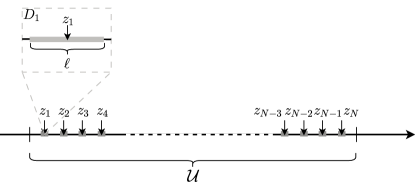
Figure 2.1: An illustration of the domain $\mathcal{U}$ with $N$ resonators.

We denote the material parameters inside the resonator $D_{i}$ by $\kappa_{\mathrm{r}}\kappa_{i}(t)$ and $\rho_{\mathrm{r}}$. We write:

$$\rho(x)=\begin{cases}\rho_{0},&x\notin{D},\\ \rho_{\mathrm{r}},&x\in D_{i},\end{cases}\qquad\kappa(x,t)=\begin{cases}\kappa_{0},&x\notin{D},\\ \kappa_{\mathrm{r}}\kappa_{i}(t),&x\in D_{i}.\end{cases}$$ (2.1)

In the acoustic setting we refer to $\rho$ as the material’s density and to $\kappa$ as the material’s bulk modulus. For our numerical simulations we shall consider

$$\kappa_{i}(t):=\frac{1}{1+\varepsilon_{\kappa,i}\cos\left(\Omega t+\phi_{\kappa,i}\right)},$$ (2.2)

for all $1\leq i\leq N$, where $\varepsilon_{\kappa,i}\in[0,1)$ are the amplitudes of the time-modulations and $\phi_{\kappa,i}\in[0,2\pi)$ the phase shifts.

Identically as in [2], we introduce the contrast parameter and the wave speeds

$$\delta:=\frac{\rho_{\mathrm{{r}}}}{\rho_{0}},\quad v_{0}:=\sqrt{\frac{\kappa_{0}}{\rho_{0}}},\quad v_{\mathrm{r}}:=\sqrt{\frac{\kappa_{\mathrm{r}}}{\rho_{\mathrm{r}}}},$$ (2.3)

respectively. We consider a wave field $u(x,t)$ given by

$$u(x,t)=\sum\limits_{n=-\infty}^{\infty}v_{n}(x)\mathrm{e}^{-\mathrm{i}(\omega+n\Omega)t},$$ (2.4)

which is furnished by the assumption that $u(x,t)\mathrm{e}^{\mathrm{i}\omega t}$ is periodic with respect to $t$ with period $T$, where $\omega$ is the frequency of the incident wave. Note that the total wave field $u$ consists the scattered wave field and the incident wave field, in particular,

$$u(x,t)=\begin{cases}u^{\mathrm{sc}}(x,t)+u^{\mathrm{in}}(x,t),&x\notin D,\\ u^{\mathrm{sc}}(x,t),&x\in D,\end{cases}$$ (2.5)

and the modes of $u^{\mathrm{sc}}(x,t)$ and $u^{\mathrm{in}}(x,t)$ are given given by $v_{n}^{\mathrm{sc}}(x)$ and $v_{n}^{\mathrm{in}}(x)$, respectively. We shall give a closed form definition of the incident wave field in Section 3.

The governing equations posed on the modes $v_{n}$, can be derived to be the following [2]:

$$\left\{\begin{array}[]{ll}\displaystyle\frac{\mathrm{d}^{2}}{\mathrm{d}x^{2}}v^{\mathrm{sc}}_{n}+\frac{\rho_{0}(\omega+n\Omega)^{2}}{\kappa_{0}}v^{\mathrm{sc}}_{n}=0,&x\notin D,\\[10.00002pt] \displaystyle\frac{\mathrm{d}^{2}}{\mathrm{d}x^{2}}v_{n}^{\mathrm{sc}}+\frac{\rho_{\mathrm{r}}(\omega+n\Omega)^{2}}{\kappa_{\mathrm{r}}}v_{i,n}^{**}=0,&x\in D_{i},\quad i=1,\ldots,N,\\[10.00002pt] \displaystyle\left.v^{\mathrm{sc}}_{n}\right|_{-}\left(x_{i}^{-}\right)-\left.v^{\mathrm{sc}}_{n}\right|_{+}\left(x_{i}^{-}\right)=v_{n}^{\mathrm{in}}|_{-}(x_{i}^{-}),&\forall\,i=1,\dots,N,\\[5.0pt] \displaystyle\left.v^{\mathrm{sc}}_{n}\right|_{-}\left(x_{i}^{+}\right)-\left.v^{\mathrm{sc}}_{n}\right|_{+}\left(x_{i}^{+}\right)=-v_{n}^{\mathrm{in}}|_{+}(x_{i}^{+}),&\forall\,i=1,\dots,N,\\[5.0pt] \displaystyle\left.\frac{\mathrm{d}v_{n}^{\mathrm{sc}}}{\mathrm{~d}x}\right|_{+}\left(x_{i}^{-}\right)-\left.\delta\frac{\mathrm{d}v^{\mathrm{sc}}_{n}}{\mathrm{d}x}\right|_{-}\left(x_{i}^{-}\right)=\left.\delta\frac{\mathrm{d}v_{n}^{\mathrm{in}}}{\mathrm{d}x}\right|_{-}(x_{i}^{-}),&\forall\,i=1,\ldots,N,\\[10.00002pt] \displaystyle\left.\frac{\mathrm{d}v_{n}^{\mathrm{sc}}}{\mathrm{~d}x}\right|_{-}\left(x_{i}^{+}\right)-\left.\delta\frac{\mathrm{d}v^{\mathrm{sc}}_{n}}{\mathrm{d}x}\right|_{+}\left(x_{i}^{+}\right)=\left.\delta\frac{\mathrm{d}v_{n}^{\mathrm{in}}}{\mathrm{d}x}\right|_{+}(x_{i}^{+}),&\forall\,i=1,\ldots,N,\\[10.00002pt] \displaystyle\left(\frac{\mathrm{d}}{\mathrm{d}|x|}-\mathrm{i}\frac{(\omega+n\Omega)}{v_{0}}\right)v^{\mathrm{sc}}_{n}=0,&x\in(-\infty,x_{1}^{-})\cup(x_{N}^{+},+\infty).\end{array}\right.$$ (2.6)

We refer to [2, Appendix A] for a detailed derivation of (2.6). The wave number corresponding to the $n$-th mode inside and outside of the resonators is defined by

$$k^{(n)}_{\mathrm{r}}:=\frac{\omega+n\Omega}{v_{\mathrm{r}}},\quad k^{(n)}:=\frac{\omega+n\Omega}{v_{0}},$$

respectively. The functions $v_{i,n}^{**}(x)$ are defined through the convolution

$$v_{i,n}^{**}(x)=\frac{1}{\omega+n\Omega}\sum_{m=-\infty}^{\infty}k_{i,m}(\omega+(n-m)\Omega)v_{n-m}(x),\quad\forall\,x\in D_{i},$$ (2.7)

where $k_{i,m}$ are the Fourier series coefficients of $1/\kappa_{i}(t)$:

$$\frac{1}{\kappa_{i}(t)}=\sum_{n=-M}^{M}k_{i,n}\mathrm{e}^{-\mathrm{i}n\Omega t}.$$

The following proposition summarises the results derived in previous papers [1, 2]:

Proposition 2.1.

The Fourier modes $v_{n}(x)$ of the wave field $u(x,t)$ solving (2.6) are given by

$$v_{n}(x)=\begin{cases}\alpha_{n}^{i}\mathrm{e}^{\mathrm{i}k^{(n)}x}+\beta_{n}^{i}\mathrm{e}^{-\mathrm{i}k^{(n)}x},&\forall\,x\in\left(x_{i-1}^{+},x_{i}^{-}\right),\\ \sum\limits_{j=-\infty}^{\infty}\left(a_{j}^{i}\mathrm{e}^{\mathrm{i}\lambda_{j}^{i}x}+b_{j}^{i}\mathrm{e}^{-\mathrm{i}\lambda_{j}^{i}x}\right)f_{n}^{j,i},&\forall\,x\in\left(x_{i}^{-},x_{i}^{+}\right),\end{cases}$$ (2.8)

where the coefficients $\alpha_{n}^{i},\,\beta_{n}^{i},\,a_{j}^{i},\,b_{j}^{i}$ need to be determined for all $i=1,\dots,N,\,j,n\in\mathbb{Z}$. The eigenpairs $\left(\lambda_{j}^{i},\mathbf{f}^{j,i}\right)_{i\in\mathbb{Z}}$ corresponding to the $i$-th resonator can be obtained as stated in [2, Lemma 2.1].

Remark 2.2.

The wave field $u(x,t)$ has infinitely many modes $v_{n}(x)$, which is problematic for the numerical implementation of the equations. Thus, we truncate the Fourier series by a truncation parameter $K\in\mathbb{N}$:

$$u(x,t)=\sum\limits_{n=-K}^{K}v_{n}(x)\mathrm{e}^{-\mathrm{i}(\omega+n\Omega)t}.$$ (2.9)

3 Static Metamaterial

In this section, we shall focus on metamaterials with static material parameters. We aim to obtain the homogenised governing equation in a manner equivalent to [5], but for a one-dimensional material. The method we introduce will be later generalised to the time-modulated case in Section˜4.

3.1 Transfer and Scattering Matrices

First we introduce the one-dimensional transfer matrix and the scattering matrix.

Proposition 3.1.

Consider the resonator $D_{i}$, and let the wave field on the left- and right-hand sides of $D_{i}$ be given by $v(x)=\alpha^{i}\mathrm{e}^{\mathrm{i}kx}+\beta^{i}\mathrm{e}^{-\mathrm{i}kx}$ and $v(x)=\alpha^{i+1}\mathrm{e}^{\mathrm{i}kx}+\beta^{i+1}\mathrm{e}^{-\mathrm{i}kx}$, respectively. Then the transfer matrix $\tilde{S}_{i}$ corresponding to $D_{i}$ is given by

$$\begin{bmatrix}\alpha^{i+1}\\ \beta^{i+1}\end{bmatrix}=\tilde{S}_{i}\begin{bmatrix}\alpha^{i}\\ \beta^{i}\end{bmatrix},$$ (3.1)

with coefficients given by

$$\tilde{S}_{i}=\begin{bmatrix}\tilde{a}_{i}&\tilde{b}_{i}\\ \tilde{c}_{i}&\tilde{d}_{i}\end{bmatrix},\quad\begin{cases}\tilde{a}_{i}:=-\frac{\mathrm{e}^{\mathrm{i}\left(k(x_{i}^{-}-x_{i}^{+})-(x_{i}^{+}+x_{i}^{-})k_{\mathrm{r}}\right)}\left(\left(\delta^{2}k^{2}+k_{\mathrm{r}}^{2}\right)\left(\mathrm{e}^{2\mathrm{i}x^{-}k_{\mathrm{r}}}-\mathrm{e}^{2\mathrm{i}x^{+}\mathrm{k}_{\mathrm{r}}}\right)-2\delta k_{\mathrm{r}}^{2}\left(\mathrm{e}^{2\mathrm{i}x^{-}k_{\mathrm{r}}}+\mathrm{e}^{2\mathrm{i}x^{+}\mathrm{k}_{\mathrm{r}}}\right)\right)}{4\delta kk_{\mathrm{r}}},\\[4.0pt] \tilde{b}_{i}:=\frac{\mathrm{e}^{-\mathrm{i}(x_{i}^{-}+x_{i}^{+})(k+k_{\mathrm{r}})}\left(\delta^{2}k^{2}-k_{\mathrm{r}}^{2}\right)\left(\mathrm{e}^{2\mathrm{i}x_{i}^{-}k_{\mathrm{r}}}-\mathrm{e}^{2\mathrm{i}x_{i}^{+}k_{\mathrm{r}}}\right)}{4\delta kk_{\mathrm{r}}},\\[4.0pt] \tilde{c}_{i}:=\frac{\mathrm{e}^{\mathrm{i}(x_{i}^{-}+x_{i}^{+})(k-k_{\mathrm{r}})}\left(-\delta^{2}k^{2}-k_{\mathrm{r}}^{2}\right)\left(\mathrm{e}^{2\mathrm{i}x_{i}^{-}k_{\mathrm{r}}}-\mathrm{e}^{2\mathrm{i}x_{i}^{+}k_{\mathrm{r}}}\right)}{4\delta kk_{\mathrm{r}}},\\[4.0pt] \tilde{d}_{i}:=\frac{\mathrm{e}^{\mathrm{i}\left(k(x_{i}^{-}-x_{i}^{+})-(x_{i}^{+}+x_{i}^{-})k_{\mathrm{r}}\right)}\left(\left(\delta^{2}k^{2}+k_{\mathrm{r}}^{2}\right)\left(\mathrm{e}^{2\mathrm{i}x^{-}k_{\mathrm{r}}}-\mathrm{e}^{2\mathrm{i}x^{+}\mathrm{k}_{\mathrm{r}}}\right)-2\delta k_{\mathrm{r}}^{2}\left(\mathrm{e}^{2\mathrm{i}x^{-}k_{\mathrm{r}}}+\mathrm{e}^{2\mathrm{i}x^{+}\mathrm{k}_{\mathrm{r}}}\right)\right)}{4\delta kk_{\mathrm{r}}}.\end{cases}$$ (3.2)

Furthermore, the scattering matrix $S_{i}$ is defined by

$$\begin{bmatrix}\alpha^{i+1}\\ \beta^{i}\end{bmatrix}=S_{i}\begin{bmatrix}\alpha^{i}\\ \beta^{i+1}\end{bmatrix},$$ (3.3)

with coefficients given by

$$S_{i}=\begin{bmatrix}a_{i}&b_{i}\\ c_{i}&d_{i}\end{bmatrix},\quad\begin{cases}a_{i}:=\tilde{a}_{i}-\frac{\tilde{b}_{i}\tilde{c}_{i}}{\tilde{d}_{i}},\\ b_{i}:=\frac{\tilde{b}_{i}}{\tilde{d}_{i}},\\ c_{i}:=-\frac{\tilde{c}_{i}}{\tilde{d}_{i}},\\ d_{i}:=\frac{1}{\tilde{d}_{i}}.\end{cases}$$ (3.4)

Proof.

If we let the interior wave field be given by $v(x)=a\mathrm{e}^{\mathrm{i}k_{\mathrm{r}}x}+b\mathrm{e}^{-\mathrm{i}k_{\mathrm{r}}x},\ x\in D_{i}$, the continuity and transmission conditions give us

$$\begin{cases}\alpha^{i}\mathrm{e}^{\mathrm{i}kx_{i}^{-}}+\beta^{i}\mathrm{e}^{-\mathrm{i}kx_{i}^{-}}=a\mathrm{e}^{\mathrm{i}k_{\mathrm{r}}x_{i}^{-}}+b\mathrm{e}^{-\mathrm{i}k_{\mathrm{r}}x_{i}^{-}},\\ \alpha^{i+1}\mathrm{e}^{\mathrm{i}kx_{i}^{+}}+\beta^{i+1}\mathrm{e}^{-\mathrm{i}kx_{i}^{+}}=a\mathrm{e}^{\mathrm{i}k_{\mathrm{r}}x_{i}^{+}}+b\mathrm{e}^{-\mathrm{i}k_{\mathrm{r}}x_{i}^{+}},\end{cases}$$ (3.5)

$$\begin{cases}\delta k\left(\alpha^{i}\mathrm{e}^{\mathrm{i}kx_{i}^{-}}-\beta^{i}\mathrm{e}^{-\mathrm{i}kx_{i}^{-}}\right)=k_{\mathrm{r}}\left(a\mathrm{e}^{\mathrm{i}k_{\mathrm{r}}x_{i}^{-}}-b\mathrm{e}^{-\mathrm{i}k_{\mathrm{r}}x_{i}^{-}}\right),\\ \delta k\left(\alpha^{i+1}\mathrm{e}^{\mathrm{i}kx_{i}^{+}}-\beta^{i+1}\mathrm{e}^{-\mathrm{i}kx_{i}^{+}}\right)=k_{\mathrm{r}}\left(a\mathrm{e}^{\mathrm{i}k_{\mathrm{r}}x_{i}^{+}}-b\mathrm{e}^{-\mathrm{i}k_{\mathrm{r}}x_{i}^{+}}\right),\end{cases}$$ (3.6)

respectively. By introducing the matrices

$$P_{i}:=\begin{bmatrix}\mathrm{e}^{\mathrm{i}kx_{i}^{+}}&\mathrm{e}^{-\mathrm{i}kx_{i}^{+}}\\ \mathrm{e}^{\mathrm{i}kx_{i}^{+}}&-\mathrm{e}^{-\mathrm{i}kx_{i}^{+}}\end{bmatrix},\quad V:=\begin{bmatrix}1&0\\ 0&\delta\frac{k}{k_{\mathrm{r}}}\end{bmatrix},\quad G_{i}:=\begin{bmatrix}\mathrm{e}^{\mathrm{i}k_{\mathrm{r}}x_{i}^{+}}&\mathrm{e}^{-\mathrm{i}k_{\mathrm{r}}x_{i}^{+}}\\ \mathrm{e}^{\mathrm{i}k_{\mathrm{r}}x_{i}^{+}}&-\mathrm{e}^{-\mathrm{i}k_{\mathrm{r}}x_{i}^{+}}\end{bmatrix},$$

$$F_{i}:=\begin{bmatrix}\mathrm{e}^{\mathrm{i}k_{\mathrm{r}}x_{i}^{-}}&\mathrm{e}^{-\mathrm{i}k_{\mathrm{r}}x_{i}^{-}}\\ \mathrm{e}^{\mathrm{i}k_{\mathrm{r}}x_{i}^{-}}&-\mathrm{e}^{-\mathrm{i}k_{\mathrm{r}}x_{i}^{-}}\end{bmatrix},\quad Q_{i}:=\begin{bmatrix}\mathrm{e}^{\mathrm{i}kx_{i}^{-}}&\mathrm{e}^{-\mathrm{i}kx_{i}^{-}}\\ \mathrm{e}^{\mathrm{i}kx_{i}^{-}}&-\mathrm{e}^{-\mathrm{i}kx_{i}^{-}}\end{bmatrix},$$

and rewriting and grouping the equations (3.5) and (3.6), we obtain

$$\tilde{S}_{i}:=P_{i}^{-1}V^{-1}G_{i}F_{i}^{-1}VQ_{i},$$ (3.7)

which is exactly (3.2). Lastly, it is a straightforward task to obtain the expression of $S_{i}$ in terms of $\tilde{S}_{i}$. ∎

With the explicit formula for $S_{i}$ at hand, we will derive a point-scattering approximation in the limit when the resonator length $\ell$ tends to zero. To fix the asymptotic regime, we will consider the subwavelength regime where $\omega=O(\ell)$ and $\delta=O(\ell)$ as $\ell\to 0$. In the remainder of this paper, we will denote the $n\times n$ identity matrix by $I_{n}$.

Lemma 3.2.

Let the $N$ resonators each be of length $\ell$ and centred around $z_{i}$, and set $\delta=\gamma\ell$ and $\omega=\mu\ell$, for fixed $\gamma,\,\mu>0$ independent of $\ell$. As $\ell\to 0$, the following holds:

$$S_{i}=I_{2}+g\begin{bmatrix}1&\mathrm{e}^{-2\mathrm{i}kz_{i}}\\ \mathrm{e}^{2\mathrm{i}kz_{i}}&1\end{bmatrix}+O(\ell^{2}),\quad\text{with}\quad g:=\frac{\mathrm{i}\ell\mu v}{2\gamma v_{\mathrm{r}}^{2}}.$$ (3.8)

Proof.

The above form of $S_{i}$ can be obtained by expanding the coefficients $a_{i},\,b_{i},\,c_{i},\,d_{i}$ in $\ell$ and omitting higher-order terms. ∎

Remark 3.3.

By plugging in (3.8) into (3.3), we obtain

$$\begin{bmatrix}\tilde{\alpha}^{i+1}\\ \tilde{\beta}^{i}\end{bmatrix}=g\begin{bmatrix}1&\mathrm{e}^{-2\mathrm{i}kz_{i}}\\ \mathrm{e}^{2\mathrm{i}kz_{i}}&1\end{bmatrix}\begin{bmatrix}\alpha^{i}\\ \beta^{i+1}\end{bmatrix},$$ (3.9)

where

$$\tilde{\alpha}^{i+1}:=\alpha^{i+1}-\alpha^{i}\quad\tilde{\beta}^{i}:=\beta^{i}-\beta^{i+1}.$$ (3.10)

The above lemma leads to an expression of the scattered wave field using the one-dimensional Helmholtz Green’s function

$$G^{k}(x-y):=\frac{\mathrm{e}^{\mathrm{i}k|x-y|}}{2\mathrm{i}k}.$$ (3.11)

Let the total wave field $u(x,t)=\mathrm{e}^{-\mathrm{i}\omega t}v(x)$ be given by

$$v(x)=\begin{cases}v^{\mathrm{sc}}(x)+v^{\mathrm{in}}(x),&x\notin D,\\ v^{\mathrm{sc}}(x),&x\in D,\end{cases}$$ (3.12)

where $v^{\mathrm{in}}(x):=\alpha^{1}\mathrm{e}^{\mathrm{i}kx}+\beta^{N+1}\mathrm{e}^{-\mathrm{i}kx}$ is the overall incident wave on the system of $N$ resonators. Moreover, we denote the incident wave field on $D_{i}$ by $v^{\mathrm{in}}_{i}(x)$ and the scattered wave field of $D_{i}$ by $v^{\mathrm{sc}}_{i}(x)$. The incident and scattered wave field of $D_{i}$ are given by

$$v_{i}^{\mathrm{in}}(x):=v^{\mathrm{in}}(x)+\sum\limits_{j\neq i}v^{\mathrm{sc}}_{j}(x),\quad v_{i}^{\mathrm{sc}}(x):=\begin{cases}\tilde{\beta}^{i}\mathrm{e}^{-\mathrm{i}kx},&x<z_{i},\\ \tilde{\alpha}^{i}\mathrm{e}^{\mathrm{i}kx},&x>z_{i}.\end{cases}$$ (3.13)

Using the definition of the Green’s function (3.11) one obtains the following characterisation:

$$v^{\mathrm{sc}}_{i}(x)=\tilde{g}G^{k}(x-z_{i})v^{\mathrm{in}}_{i}(z_{i}),$$ (3.14)

where $\tilde{g}:=2\mathrm{i}kg$, with $g$ as defined in Lemma 3.2. Equation (3.14) is a point-scattering approximation for a static resonator, which characterises the scattered wave from $D_{i}$ in terms of the Green’s function. This formula sets the ground to derive the homogenised equation equivalently as in [5].

3.2 Homogenised Equation

In this section, we shall obtain the homogenised equation using our previous results. First, we substitute the scattered wave field of $D_{i}$ (3.14) into the incident wave field (3.13) of $D_{i}$ and evaluate at $z_{i}$:

$$v^{\mathrm{in}}_{i}(z_{i})=v^{\mathrm{in}}(z_{i})+\sum\limits_{j\neq i}\tilde{g}G^{k}(z_{i}-z_{j})v^{\mathrm{in}}_{j}(z_{j}).$$ (3.15)

Equation (3.15) is a linear system of equations: define the vectors $\mathbf{x},\,\mathbf{b}\in\mathbb{C}^{N}$ and the matrix $T\in\mathbb{C}^{N\times N}$ with entries

$$x_{i}:=v^{\mathrm{in}}_{i}(z_{i}),\quad b_{i}:=v^{\mathrm{in}}(z_{i}),\quad T_{ij}:=\begin{cases}\tilde{g}G^{k}(z_{i}-z_{j}),&i\neq j,\\ 0,&i=j,\end{cases}$$ (3.16)

then (3.15) leads to the following:

$$\mathbf{x}-T\mathbf{x}=\mathbf{b}.$$ (3.17)

In order to homogenise our system, we must assume that while the number of resonators grows, they are still well-separated, which means that their size simultaneously decreases. In other words, we consider an asymptotic regime where the volume fraction of resonators is fixed.

Assumption 3.4.

Assume that there exists a constant $\Lambda>0$ such that $N\ell=\Lambda$, for all $N,\,\ell>0$.

Next, we have

$$\tilde{g}=\frac{\mathrm{i}\ell\mu v}{2\gamma v_{\mathrm{r}}^{2}}\frac{2\mathrm{i}\mu\ell}{v}=-\frac{1}{N}\frac{\mu^{2}\ell}{\gamma v_{\mathrm{r}}^{2}}\Lambda=:\frac{1}{N}\beta\Lambda.$$ (3.18)

Hence, we can conclude that

$$v^{\mathrm{in}}_{i}(z_{i})=v^{\mathrm{in}}(z_{i})+\frac{1}{N}\sum\limits_{j\neq i}\beta\Lambda G^{k}(z_{i}-z_{j})v^{\mathrm{in}}_{j}(z_{j}).$$ (3.19)

Following [5], we introduce the limiting density $\tilde{V}(x)$ of resonators.

Assumption 3.5.

Let $A\subset\mathbb{R}$ be a measurable set, we define

$$\Theta^{N}(A):=\frac{1}{N}\times\{\text{number of points }z_{i}\in A\}.$$ (3.20)

Assume that there exists $\tilde{V}\in L^{\infty}(\mathcal{U})$ such that

$$\Theta^{N}(A)\to\int_{A}\tilde{V}(x)\,\mathrm{d}x\quad\text{as }N\to\infty.$$ (3.21)

We define the $L^{\infty}$-function $V(x):=\beta\Lambda\tilde{V}(x)$. The following assumption is feasible based on [5, Lemma 4.1].

Assumption 3.6.

We assume that for any $f\in C^{0,\alpha}(\mathcal{U})$

$$\max_{1\leq i\leq N}\left|\frac{1}{N}\sum\limits_{j\neq i}\beta\Lambda G^{k}(z_{i}-z_{j})f(z_{j})-\int_{\mathcal{U}}G^{k}(z_{i}-y)V(y)f(y)\,\mathrm{d}y\right|\leq\frac{C}{N^{\alpha/3}}||f||_{C^{0,\alpha}(\mathcal{U})},$$ (3.22)

for some constants $0<\alpha<1$ and $C>0$.

We now define the operator $\mathcal{T}:C^{0,\alpha}(\mathcal{U})\to C^{0,\alpha}(\mathcal{U})$ by

$$\mathcal{T}f(x):=\int_{\mathcal{U}}G^{k}(x-y)V(y)f(y)\,\mathrm{d}y.$$ (3.23)

Analogously as in [5], this operator can be seen as the continuum limit of the matrix operator $T$. Since we define $\mathcal{T}$ in an equivalent manner as in the higher-dimensional case, the properties proven in [5, Lemma 4.2] still hold true in one dimension.

Let $v^{i}\in C^{0,\alpha}(\mathcal{U})$, if $\psi$ is the unique solution of $\psi-\mathcal{T}\psi=v^{i}$, then

$$\left(\frac{\mathrm{d}^{2}}{\mathrm{d}x^{2}}+k^{2}\right)\psi-V\psi=0\quad\text{in }\mathbb{R},$$ (3.24)

which is exactly the homogenised equation. Similarly as in [5], it can be proven that $\psi$ is the continuum limit of the solution $\mathbf{x}$ to (3.17).

4 Time-dependent Metamaterial

In this section, we focus on time-dependent materials and obtain a homogenised equation. For that, we follow an equivalent approach as in Section 3. Note that, as explained in Remark 2.2, we work with a truncated system with Fourier series of length $K$.

Our aim is first to define the transfer and scattering matrix for time-dependent materials. To do so, we write out the continuity conditions and transmission conditions:

$$\begin{cases}\alpha^{i}_{n}\mathrm{e}^{\mathrm{i}k^{(n)}x_{i}^{-}}+\beta^{i}_{n}\mathrm{e}^{-\mathrm{i}k^{(n)}x_{i}^{-}}=\sum\limits_{j=-K}^{K}\left(a_{j}^{i}\mathrm{e}^{\mathrm{i}\lambda_{j}^{i}x_{i}^{-}}+b_{j}^{1}\mathrm{e}^{-\mathrm{i}\lambda_{j}^{i}x_{i}^{-}}\right)f_{n}^{j,i},\\ \alpha^{i+1}_{n}\mathrm{e}^{\mathrm{i}k^{(n)}x_{i}^{+}}+\beta^{i+1}_{n}\mathrm{e}^{-\mathrm{i}k^{(n)}x_{i}^{+}}=\sum\limits_{j=-K}^{K}\left(a_{j}^{i}\mathrm{e}^{\mathrm{i}\lambda_{j}^{i}x_{i}^{+}}+b_{j}^{1}\mathrm{e}^{-\mathrm{i}\lambda_{j}^{i}x_{i}^{+}}\right)f_{n}^{j,i},\end{cases}$$ (4.1)

$$\begin{cases}\delta k^{(n)}\left(\alpha^{i}_{n}\mathrm{e}^{\mathrm{i}k^{(n)}x_{i}^{-}}-\beta^{i}_{n}\mathrm{e}^{-\mathrm{i}k^{(n)}x_{i}^{-}}\right)=\sum\limits_{j=-K}^{K}\left(a_{j}^{i}\mathrm{e}^{\mathrm{i}\lambda_{j}^{i}x_{i}^{-}}-b_{j}^{1}\mathrm{e}^{-\mathrm{i}\lambda_{j}^{i}x_{i}^{-}}\right)\lambda_{j}^{i}f_{n}^{j,i},\\ \delta k^{(n)}\left(\alpha^{i+1}_{n}\mathrm{e}^{\mathrm{i}k^{(n)}x_{i}^{+}}-\beta^{i+1}_{n}\mathrm{e}^{-\mathrm{i}k^{(n)}x_{i}^{+}}\right)=\sum\limits_{j=-K}^{K}\left(a_{j}^{i}\mathrm{e}^{\mathrm{i}\lambda_{j}^{i}x_{i}^{+}}-b_{j}^{1}\mathrm{e}^{-\mathrm{i}\lambda_{j}^{i}x_{i}^{+}}\right)\lambda_{j}^{i}f_{n}^{j,i},\end{cases}$$ (4.2)

for all $n=-K,\dots,K$. Next, we define a matrix $F_{i}:=\left(f_{n}^{j,i}\right)_{n,j=-K}^{K}$ and its inverse $G_{i}:=F_{i}^{-1}$. We will rewrite the above four equations, which hold for all $n=-K,\dots,K$, into a single matrix equation. We introduce the following notation for the unknown coefficients:

$$\boldsymbol{\alpha}^{i}:=\begin{bmatrix}\alpha^{i}_{-K}\\ \vdots\\ \alpha_{K}^{i}\end{bmatrix},\quad\boldsymbol{\beta}^{i}:=\begin{bmatrix}\beta^{i}_{-K}\\ \vdots\\ \beta^{i}_{K}\end{bmatrix},\quad\mathbf{w}^{i}:=\begin{bmatrix}\boldsymbol{\alpha}^{i}\\ \boldsymbol{\beta}^{i}\end{bmatrix},\quad\mathbf{v}_{j}^{i}:=\begin{bmatrix}a_{j}^{i}\\ b_{j}^{i}\end{bmatrix},\quad\mathbf{v}^{i}:=\begin{bmatrix}\mathbf{v}_{-K}^{i}\\ \vdots\\ \mathbf{v}_{K}^{i}\end{bmatrix}.$$ (4.3)

For the sake of simplicity, we omit the indices $i$ in the following notation. Then we introduce the matrices

$$E_{\pm}:=\mathrm{diag}\left(\mathrm{e}^{\pm\mathrm{i}k^{(n)}x^{+}}\right)_{n=-K}^{K},\quad K:=\mathrm{diag}\left(k^{(n)}\right)_{n=-K}^{K},$$ (4.4)

$$T^{\pm}:=\mathrm{diag}\left(\left[\mathrm{e}^{\mathrm{i}\lambda_{j}^{i}x^{\pm}},\,\mathrm{e}^{-\mathrm{i}\lambda_{j}^{i}x^{\pm}}\right]\right)_{j=-K}^{K},\quad T^{\pm}_{\lambda}:=\mathrm{diag}\left(\left[\lambda_{j}^{i}\mathrm{e}^{\mathrm{i}\lambda_{j}^{i}x^{\pm}},\,-\lambda_{j}^{i}\mathrm{e}^{-\mathrm{i}\lambda_{j}^{i}x^{\pm}}\right]\right)_{j=-K}^{K},$$ (4.5)

$$\mathcal{M}^{-}:=\begin{bmatrix}GE_{-}&GE_{+}\\ \delta GKE_{-}&-\delta GKE_{+}\end{bmatrix},\quad\mathcal{T}^{-}:=\begin{bmatrix}T^{-}\\ T^{-}_{\lambda}\end{bmatrix},\quad\mathcal{M}^{+}:=\begin{bmatrix}E_{+}&E_{-}\\ \delta KE_{+}&-\delta KE_{-}\end{bmatrix},\quad\mathcal{T}^{+}:=\begin{bmatrix}FT^{+}\\ FT^{+}_{\lambda}\end{bmatrix}.$$ (4.6)

With this notation it can be proven that (4.1) and (4.2) are equivalent to

$$\mathcal{M}^{-}\mathbf{w}^{i}=\mathcal{T}\mathbf{v}^{i},\quad\mathcal{M}^{+}\mathbf{w}^{i+1}=\mathcal{T}^{+}\mathbf{v}^{i}.$$ (4.7)

We have now transformed the four equations (4.1) and (4.2) that are true for each $n$ into two linear systems of equations, which contain all the modes $n$. By combining the two equations into a single one, we arrive at the following proposition, which defines the time-dependent scattering matrix. We assume that $\omega$ is not a multiple of $\Omega$, whereby a direct calculation shows that $\mathcal{M}^{+}$ and $\mathcal{T}^{-}$ are invertible.

Proposition 4.1.

Consider the resonator $D_{i}$, and assume that $\omega\neq m\Omega$ for all $m\in\mathbb{Z}$. Let the wave field on the left side of $D_{i}$ be given by the modes $v_{n}(x)=\alpha^{i}_{n}\mathrm{e}^{\mathrm{i}k^{(n)}x}+\beta^{i}_{n}\mathrm{e}^{-\mathrm{i}k^{(n)}x}$ and the wave field on the right side of $D_{i}$ be given by the modes $v_{n}(x)=\alpha^{i+1}_{n}\mathrm{e}^{\mathrm{i}k^{(n)}x}+\beta^{i+1}_{n}\mathrm{e}^{-\mathrm{i}k^{(n)}x}$. Then the corresponding transfer matrix is given by

$$\mathbf{w}^{i+1}=\tilde{S}_{i}\mathbf{w}^{i},\quad\tilde{S}_{i}:=\left(\mathcal{M}^{+}\right)^{-1}\mathcal{T}^{+}\left(\mathcal{T}^{-}\right)^{-1}\mathcal{M}^{-}=:\begin{bmatrix}\tilde{S}_{11}&\tilde{S}_{12}\\ \tilde{S}_{21}&\tilde{S}_{22}\end{bmatrix}\in\mathbb{C}^{2(2K+1)\times 2(2K+1)},$$ (4.8)

where these matrices are defined in (4.6). Furthermore, the scattering matrix is defined by

$$S_{i}:=\begin{bmatrix}S_{11}&S_{12}\\ S_{21}&S_{22}\end{bmatrix},\quad\begin{cases}S_{11}:=\tilde{S}_{11}-\tilde{S}_{12}\tilde{S}_{22}^{-1}\tilde{S}_{21},\\ S_{12}:=\tilde{S}_{12}\tilde{S}_{22}^{-1},\\ S_{21}:=-\tilde{S}_{22}^{-1}\tilde{S}_{21},\\ S_{22}:=\tilde{S}_{22}^{-1},\end{cases}$$ (4.9)

and it satisfies

$$\begin{bmatrix}\boldsymbol{\alpha}^{i+1}\\ \boldsymbol{\beta}^{i}\end{bmatrix}=S_{i}\begin{bmatrix}\boldsymbol{\alpha}^{i}\\ \boldsymbol{\beta}^{i+1}\end{bmatrix}.$$ (4.10)

As in the previous section, we proceed by taking the limit $\ell\to 0$ and derive a point-scattering approximation equivalent to Lemma 3.2. We take the same asymptotic scaling as before, whereby $\delta=\gamma\ell,\,\omega=\mu\ell,\,\Omega=\xi\ell,$ and $\lambda_{j}^{i}=c_{j}^{i}\ell$, for fixed $\gamma,\,\mu,\,\xi>0$ independent of $\ell$. Here, recall that $\lambda_{j}^{i}$ are the wave numbers in the $i$^th resonator, as in ˜2.1. Note that the exact definition of $c_{j}^{i}$ depends on $\mu$ and $\Omega$. Although there is no closed-form expression for these coefficients, they can be efficiently computed as the eigenvalues of the temporal Sturm-Liouville problem in the interior of $D_{i}$ (see, for example, [1, Lemma III.3] or [13, Section V]).

Lemma 4.2.

Let the $N$ resonators each be of length $\ell$ and centred around $z_{i}$, and set $\delta=\gamma\ell,\,\omega=\mu\ell,\,\Omega=\xi\ell,\,\lambda_{j}^{i}=c_{j}^{i}\ell$, for fixed $\gamma,\,\mu,\,\xi>0$ independent of $\ell$. Assume that $\omega\neq m\Omega$ for all $m\in\mathbb{Z}$. Then, as $\ell\to 0$, the following holds:

$$S_{i}=\begin{bmatrix}I_{2K+1}&0\\ 0&I_{2K+1}\end{bmatrix}+\begin{bmatrix}g^{i}&0\\ 0&g^{i}\end{bmatrix}\begin{bmatrix}I_{2K+1}&\mathrm{diag}\left(\mathrm{e}^{-2\mathrm{i}k^{(n)}z_{i}}\right)_{n=-K}^{K}\\ \mathrm{diag}\left(\mathrm{e}^{2\mathrm{i}k^{(n)}z_{i}}\right)_{n=-K}^{K}&I_{2K+1}\end{bmatrix}+O(\ell^{2}),$$ (4.11)

where $g^{i}\in\mathbb{C}^{(2K+1)\times(2K+1)}$ is given by

$$g^{i}:=\left(I_{2K+1}-\mathcal{A}_{i}\right)^{-1}\mathcal{A}_{i},\quad\mathcal{A}_{i}:=\frac{\ell}{2\gamma}\mathrm{diag}\left(\frac{v}{\mu+n\xi}\right)_{n=-K}^{K}F\mathrm{diag}\left(\mathrm{i}(c_{j}^{i})^{2}\right)_{j=-K}^{K}G.$$ (4.12)

For the proof of Lemma 4.2 we shall use the following well-known result from linear algebra:

Lemma 4.3.

The inverse of an invertible $2m\times 2m$ matrix

$$M=\begin{bmatrix}A&B\\ C&D\end{bmatrix},$$ (4.13)

with blocks $A,\,B,\,C,\,D\in\mathbb{C}^{m\times m}$ is given by

$$M^{-1}=\begin{bmatrix}A^{-1}+A^{-1}BS^{-1}CA^{-1}&-A^{-1}BS^{-1}\\ -S^{-1}CA^{-1}&S^{-1}\end{bmatrix},\quad S:=D-CA^{-1}B,$$ (4.14)

provided that $A$ and $S$ are invertible. Note that $S$ is called the Schur complement of $A$.

With the result of Lemma 4.3, we can now prove Lemma 4.2.

Proof of Lemma 4.2.

Recall that the transfer matrix is given by $\tilde{S}_{i}:=\left(\mathcal{M}^{+}\right)^{-1}\mathcal{T}^{+}\left(\mathcal{T}^{-}\right)^{-1}\mathcal{M}^{-}$, as defined in (4.6). The proof will consist of simplifying each term appearing in $\tilde{S}_{i}$ and then taking the limit $\ell\to 0$.

Invert $\mathcal{M}^{+}$:
The Schur complement of the first block of $\mathcal{M}^{+}$ is given by

$$S_{\mathcal{M}^{+}}=-\delta KE_{-}-(\delta KE_{+})\left(E_{+}\right)^{-1}E_{-}=-2\delta KE_{-}\quad\implies\quad S_{\mathcal{M}^{+}}^{-1}=-\frac{1}{2\delta}E_{+}K^{-1}.$$ (4.15)

Then, by Lemma 4.3, the inverse of $\mathcal{M}^{+}$ is given by

$$\left(\mathcal{M}^{+}\right)^{-1}=\frac{1}{2}\begin{bmatrix}E_{-}&\frac{1}{\delta}E_{-}K^{-1}\\ E_{+}&-\frac{1}{\delta}E_{+}K^{-1}\end{bmatrix}.$$ (4.16)

Invert $\mathcal{T}^{-}$:
The inverse of $\mathcal{T}^{-}$ can be computed to be given by

$$\left(\mathcal{T}^{-}\right)^{-1}=\begin{bmatrix}\hat{T}&\hat{T}_{\lambda}\end{bmatrix},\quad\hat{T}:=\mathrm{diag}\left(\frac{1}{2}\begin{bmatrix}\mathrm{e}^{-\mathrm{i}\lambda_{j}^{i}x^{-}}\\ \mathrm{e}^{\mathrm{i}\lambda_{j}^{i}x^{-}}\end{bmatrix}\right)_{j=-K}^{K},\quad\hat{T}_{\lambda}:=\mathrm{diag}\left(\frac{1}{2\lambda_{j}^{i}}\begin{bmatrix}\mathrm{e}^{-\mathrm{i}\lambda_{j}^{i}x^{-}}\\ -\mathrm{e}^{\mathrm{i}\lambda_{j}^{i}x^{-}}\end{bmatrix}\right)_{j=-K}^{K}.$$ (4.17)

Multiply $\mathcal{T}^{+}$ by $\left(\mathcal{T}^{-}\right)^{-1}$:
Recall that $\mathcal{T}^{+}$ is given by

$$\mathcal{T}^{+}=\begin{bmatrix}FT^{+}\\ FT^{+}_{\lambda}\end{bmatrix}=\underbrace{\begin{bmatrix}F&0\\ 0&F\end{bmatrix}}_{=:\mathcal{F}}\begin{bmatrix}T^{+}\\ T^{+}_{\lambda}\end{bmatrix}.$$ (4.18)

Then one obtains

$$\mathcal{T}^{+}\left(\mathcal{T}^{-}\right)^{-1}=\mathcal{F}\begin{bmatrix}T^{+}\hat{T}&T^{+}\hat{T}_{\lambda}\\ T^{+}_{\lambda}\hat{T}&T^{+}_{\lambda}\hat{T}_{\lambda}\end{bmatrix}.$$ (4.19)

Simplify $\mathcal{M}^{-}$:
The matrix $\mathcal{M}^{-}$ can be written as

$$\mathcal{M}^{-}=\underbrace{\begin{bmatrix}G&0\\ 0&G\end{bmatrix}}_{=:\mathcal{G}}\begin{bmatrix}E_{-}&E_{+}\\ \delta KE_{-}&-\delta KE_{+}\end{bmatrix}.$$ (4.20)

Compute $\tilde{S}_{i}$:
Finally, the transfer matrix can be written out as

$$\tilde{S}_{i}=\frac{1}{2}\begin{bmatrix}E_{-}&\frac{1}{\delta}E_{-}K^{-1}\\ E_{+}&-\frac{1}{\delta}E_{+}K^{-1}\end{bmatrix}\mathcal{F}\begin{bmatrix}T^{+}\hat{T}&T^{+}\hat{T}_{\lambda}\\ T^{+}_{\lambda}\hat{T}&T^{+}_{\lambda}\hat{T}_{\lambda}\end{bmatrix}\mathcal{G}\begin{bmatrix}E_{-}&E_{+}\\ \delta KE_{-}&-\delta KE_{+}\end{bmatrix},$$ (4.21)

and through some calculations one can achieve the following explicit definitions of the four submatrices of $\tilde{S}_{i}$:

$$\tilde{S}_{11}=\frac{1}{2}\left(\left(E_{-}F(T^{+}\hat{T})+\frac{1}{\delta}E_{-}K^{-1}F(T^{+}_{\lambda}\hat{T})\right)GE_{-}+\left(\delta E_{-}F(T^{+}\hat{T}_{\lambda})+E_{-}K^{-1}F(T^{+}_{\lambda}\hat{T}_{\lambda})\right)GKE_{-}\right),$$

$$\tilde{S}_{12}=\frac{1}{2}\left(\left(E_{-}F(T^{+}\hat{T})+\frac{1}{\delta}E_{-}K^{-1}F(T^{+}_{\lambda}\hat{T})\right)GE_{+}-\left(\delta E_{-}F(T^{+}\hat{T}_{\lambda})+E_{-}K^{-1}F(T^{+}_{\lambda}\hat{T}_{\lambda})\right)GKE_{+}\right),$$

$$\tilde{S}_{21}=\frac{1}{2}\left(\left(E_{+}F(T^{+}\hat{T})-\frac{1}{\delta}E_{+}K^{-1}F(T^{+}_{\lambda}\hat{T})\right)GE_{-}+\left(\delta E_{+}F(T^{+}\hat{T}_{\lambda})-E_{+}K^{-1}F(T^{+}_{\lambda}\hat{T}_{\lambda})\right)GKE_{-}\right),$$

$$\tilde{S}_{22}=\frac{1}{2}\left(\left(E_{+}F(T^{+}\hat{T})-\frac{1}{\delta}E_{+}K^{-1}F(T^{+}_{\lambda}\hat{T})\right)GE_{+}-\left(\delta E_{+}F(T^{+}\hat{T}_{\lambda})-E_{+}K^{-1}F(T^{+}_{\lambda}\hat{T}_{\lambda})\right)GKE_{+}\right).$$

Let $\ell\to 0$:
We now want to compute the leading order terms of $\tilde{S}_{ij}$, as $\ell\to 0$. One can prove

$$T^{+}\hat{T}=I_{2K+1}+O(\ell^{4}),\quad T^{+}_{\lambda}\hat{T}=\mathrm{diag}\left(\mathrm{i}(c_{j}^{i})^{2}\right)_{j=-K}^{K}\ell^{3}+O(\ell^{4}),\quad T^{+}_{\lambda}\hat{T}_{\lambda}=I_{2K+1}+O(\ell^{4}),$$

and that $E_{\pm}=I_{2K+1}+O(\ell)$. Plugging these asymptotic formulas into $\tilde{S}_{ij}$ and neglecting higher order terms, we obtain

$$\begin{cases}\tilde{S}_{11}=I_{2K+1}+\mathcal{A}_{i}+O(\ell^{2}),\\ \tilde{S}_{12}=\mathcal{A}_{i}+O(\ell^{2}),\\ \tilde{S}_{21}=-\mathcal{A}_{i}+O(\ell^{2}),\\ \tilde{S}_{22}=I_{2K+1}-\mathcal{A}_{i}+O(\ell^{2}),\end{cases}$$ (4.22)

with $\mathcal{A}_{i}$ defined by (4.12). If we then define $g^{i}=\left(I_{2K+1}-\mathcal{A}_{i}\right)^{-1}\mathcal{A}_{i}$ and use the formulas (4.9), we obtain the desired result (4.11). ∎

We now want to use the asymptotic result of Lemma 4.2 in order to characterise the total wave field as $\ell\to 0$. Let us separate the total wave field as a sum of incident and scattered fields

$$v_{n}(x)=\begin{cases}v_{n}^{\mathrm{sc}}(x)+v_{n}^{\mathrm{in}}(x),&x\notin D,\\ v_{n}^{\mathrm{sc}}(x),&x\in D,\end{cases}$$ (4.23)

where $v_{n}^{\mathrm{in}}(x):=\alpha^{1}_{n}\mathrm{e}^{\mathrm{i}k^{(n)}x}+\beta^{N+1}_{n}\mathrm{e}^{-\mathrm{i}k^{(n)}x}$. The scattered wave field emerging from $D_{i}$ is given by

$$v^{\mathrm{sc}}_{i,n}(x)=G^{k^{(n)}}(x-z_{i})\sum\limits_{m=-K}^{K}\tilde{g}^{i}_{nm}v_{i,m}^{\mathrm{in}}(z_{i}),$$ (4.24)

where $\tilde{g}^{i}_{nm}:=2\mathrm{i}k^{(n)}g^{i}_{nm}$ and we use the notation $g^{i}:=\left(g^{i}_{nm}\right)_{m,n=-K}^{K}$. Here, $v_{i,m}^{\mathrm{in}}$ is the field which is incident to $D_{i}$, and the scattered field is defined piecewise by

$$v^{\mathrm{sc}}_{n}(x):=\sum\limits_{i=1}^{N}v^{\mathrm{sc}}_{i,n}(x).$$ (4.25)

Furthermore, the wave field impinging on $D_{i}$ is given by

$$v^{\mathrm{in}}_{i,n}(x)=v^{\mathrm{in}}_{n}(x)+\sum\limits_{j\neq i}v_{j,n}^{\mathrm{sc}}(x)=v^{\mathrm{in}}_{n}(x)+\sum\limits_{j\neq i}\sum\limits_{m=-K}^{K}\tilde{g}^{j}_{nm}v^{\mathrm{in}}_{j,m}(z_{j})G^{k^{(n)}}(x-z_{j}).$$ (4.26)

Note that the characterisations (4.24) and (4.26) hold true only as $\ell\to 0$ and can be derived using the results proven in Lemma 4.2.

4.1 Homogenised Equation

To obtain the time-dependent homogenised equation, we first evaluate (4.26) at each resonator $z_{i}$:

$$v^{\mathrm{in}}_{i,n}(z_{i})=v^{\mathrm{in}}_{n}(z_{i})+\sum\limits_{j\neq i}v_{j,n}^{\mathrm{sc}}(z_{i})=v^{\mathrm{in}}_{n}(z_{i})+\sum\limits_{j\neq i}\sum\limits_{m=-K}^{K}\tilde{g}^{j}_{nm}v^{\mathrm{in}}_{j,m}(z_{j})G^{k^{(n)}}(z_{i}-z_{j}),$$ (4.27)

for all $i=1,\dots,N$ and $n=-K,\dots,K$. Now we define the vectors $\mathbf{x},\mathbf{b}\in\mathbb{C}^{N(2K+1)}$ with entries

$$\mathbf{x}=\begin{bmatrix}v^{\mathrm{in}}_{1,-K}(z_{1})\\ \vdots\\ v^{\mathrm{in}}_{1,K}(z_{1})\\ \vdots\\ v^{\mathrm{in}}_{N,-K}(z_{N})\\ \vdots\\ v^{\mathrm{in}}_{N,K}(z_{N})\end{bmatrix},\quad\mathbf{b}=\begin{bmatrix}v^{\mathrm{in}}_{-K}(z_{1})\\ \vdots\\ v^{\mathrm{in}}_{K}(z_{1})\\ \vdots\\ v^{\mathrm{in}}_{-K}(z_{N})\\ \vdots\\ v^{\mathrm{in}}_{K}(z_{N})\end{bmatrix}$$ (4.28)

and let the matrix $T\in\mathbb{C}^{N(2K+1)\times N(2K+1)}$ be defined by

$$T^{ij}_{nm}:= \begin{cases}\tilde{g}_{mn}^{j}G^{k^{(m)}}(z_{i}-z_{j}),&i\neq j,\\ 0,&i=j,\end{cases}\qquad T:=\begin{bmatrix}\begin{bmatrix}T^{ij}_{nm}\end{bmatrix}_{n,m=-K}^{K}\end{bmatrix}_{i,j=1}^{N}.$$ (4.29)

This notation allow us to rewrite (4.27) as

$$\mathbf{x}-T\mathbf{x}=\mathbf{b},$$ (4.30)

which is of the same form as in the static case (3.17), but where the linear system has a block structure. As in the static case, we must pose some assumptions in order to derive the homogenised equation.

Assumption 4.4.

Assume that $\kappa_{i}(t)\equiv\kappa(t)$ is identical across all resonators. Therefore, $\lambda^{i}_{j}=c^{i}_{j}\ell\equiv c_{j}\ell$ and as a consequence, $g^{i}_{mn}\equiv g_{mn}$.

We also impose the assumptions of the previous section: ˜3.4 (constant volume fraction), ˜3.5 (limiting density $\tilde{V}(x)$), and ˜3.6 (continuum limit approximation). This allow us to write

$$\tilde{g}_{nm}=2\mathrm{i}k^{(n)}g_{nm}=\frac{2\mathrm{i}}{N}\frac{\mu+n\xi}{v}\Lambda g_{nm}=:\frac{1}{N}\beta_{nm}\Lambda.$$ (4.31)

The definition of $\beta_{nm}$ was obtained in the same way as in the static case (3.18). Recall that $g^{i}_{nm}$ defined by (4.12) does not depend on $\ell$ and therefore, $\beta^{i}_{nm}$ does not depend on $\ell$ nor $N$. Hence,

$$v^{\mathrm{in}}_{i,n}(z_{i})=v^{\mathrm{in}}_{n}(z_{i})+\frac{1}{N}\sum\limits_{j\neq i}\sum\limits_{m=-K}^{K}\beta_{nm}\Lambda v^{\mathrm{in}}_{i,n}(z_{j})G^{k^{(n)}}(z_{i}-z_{j}).$$ (4.32)

Lemma 4.5.

For any $f_{m}\in C^{0,\alpha}(\mathcal{U})$ with $0<\alpha\leq 1$,

$$\max\limits_{1\leq i\leq N}\Bigg{|}\frac{1}{N}\sum\limits_{j\neq i}\sum\limits_{m=-K}^{K}\beta_{nm}\Lambda G^{k^{(n)}}(z_{i}-z_{j})f_{m}(z_{j})- \int_{\mathcal{U}}\sum\limits_{m=-K}^{K}G^{k^{(n)}}(z_{i}-y)V_{nm}(y)f_{m}(y)\,\mathrm{d}y\Bigg{|}$$

$$\leq\sum\limits_{m=-K}^{K}\frac{C_{nm}}{N^{\alpha/3}}||f_{m}||_{C^{0,\alpha}(\mathcal{U})},$$ (4.33)

for all $n=-K,\dots,K$.

Proof.

First, define $V_{nm}(x):=\beta_{nm}\Lambda\tilde{V}(x)$, for $\tilde{V}$ defined through (3.21). We use Assumption 3.6 to obtain the desired result. ∎

Next, define the operators $\mathcal{T}^{nm}:C^{0,\alpha}(\mathcal{U})\to C^{0,\alpha}(\mathcal{U})$ by

$$\mathcal{T}^{nm}f(x)=\int_{\mathcal{U}}G^{k^{(n)}}(x-y)V_{nm}(y)f(y)\,\mathrm{d}y,\quad\forall\,m,n=-K,\dots,K.$$ (4.34)

By substituting the above defined integral operator $\mathcal{T}^{nm}$ into Lemma 4.5, applying it to (4.32), and neglecting the remainder term, we obtain a system of coupled Lippmann-Schwinger equations

$$\psi_{n}+\sum_{m=-K}^{K}\mathcal{T}^{nm}\psi_{m}=\psi^{\mathrm{in}},\quad\forall\,n=-K,\dots,K.$$ (4.35)

Then, applying the operator $\left(\frac{\mathrm{d}^{2}}{\mathrm{d}x^{2}}+\left(k^{(n)}\right)^{2}\right)$ leads to the homogenised equations

$$\left(\frac{\mathrm{d}^{2}}{\mathrm{d}x^{2}}+\left(k^{(n)}\right)^{2}\right)\psi_{n}(x)-V_{nn}(x)\psi_{n}(x)\\ -\sum\limits_{m=-K}^{K}\left(\left(k^{(m)}\right)^{2}-\left(k^{(n)}\right)^{2}\right)\int_{\mathcal{U}}G^{k^{(n)}}(x-y)V_{nm}(y)\psi_{m}(y)\,\mathrm{d}y=0.$$ (4.36)

Remark 4.6.

Note that ${\psi}_{n}(z_{i})$ is the continuum limit of ${v}^{\mathrm{in}}_{i,n}$ as $N\to\infty$, which is proved in detail for the higher-dimensional static case in [5]. Looking at (4.23) and (4.27), the total field is given by $v^{\mathrm{in}}_{i,n}+v^{\mathrm{sc}}_{i,n}=v_{n}$ for all $i=1,\dots,N$. However, as $N\to\infty$, the scattered field of a single resonator $v_{i,n}^{\mathrm{sc}}$ becomes negligible. Thus, ${\psi}_{n}$ is the continuum limit of the total wave field $v_{n}$.

Corollary 4.7.

The system of homogenised equations (4.36) can be rewritten into a single vector-valued equation given by

$$\mathrm{diag}\left(\frac{\mathrm{d}^{2}}{\mathrm{d}x^{2}}+\left(k^{(n)}\right)^{2}\right)_{n=-K}^{K}\boldsymbol{\psi}(x)-\mathrm{diag}\left(V_{nn}(x)\right)_{n=-K}^{K}\boldsymbol{\psi}(x)-\int_{\mathcal{U}}\mathcal{A}(x,y)\boldsymbol{\psi}(y)\,\mathrm{d}y=\mathbf{0},$$ (4.37)

for the vector $\boldsymbol{\psi}:=\left(\psi_{n}\right)_{n=-K}^{K}$ and the matrix $\mathcal{A}(x,y):=\left(\mathcal{A}_{nm}(x,y)\right)_{m,n=-K}^{K}$ with entries

$$\mathcal{A}_{nm}(x,y):=\begin{cases}0,&n=m,\\ \left(\left(k^{(m)}\right)^{2}-\left(k^{(n)}\right)^{2}\right)G^{k^{(n)}}(x-y)V_{nm}(y),&n\neq m.\end{cases}$$ (4.38)

Corollary 4.8.

The system of coupled equations (4.35) can be rewritten into a single vector Lippmann-Schwinger equation given by

$$\boldsymbol{\psi}(x)=\mathbf{v}^{\mathrm{in}}(x)+\int_{\mathcal{U}}\mathcal{V}(x,y)\boldsymbol{\psi}(y)\,\mathrm{d}y,$$ (4.39)

where

$$\mathcal{V}(x,y):=\left(\mathcal{V}_{nm}(x,y)\right)_{n,m=-K}^{K},\quad\mathcal{V}_{nm}(x,y):=G^{k^{(n)}}(x-y)V_{nm}(y).$$ (4.40)

˜4.7 and ˜4.8 are the main results of the homogenisation. They provide two equivalent formulations of the effective field $\boldsymbol{\psi}$ emerging from a homogenised time-dependent material. Comparing the homogenised equation (4.37) to the static case in (3.24), we observe that the time-modulated case is described by an integro-differential homogenised equation, rather than a differential equation.

Remark 4.9.

As pointed out in [5], we note that it is not possible to obtain an effective medium theory for frequencies that are too close to the resonant frequency of a high-contrast resonator. In this case, the scattering matrix $g$ is of order one as $\ell\to 0$. Each additional resonator therefore yields a strong contribution to the total field. The limit as $N\to\infty$ does not exist and homogenisation is not possible.

To justify the asymptotic regime used in Section˜4, we use the formulas for the resonant frequencies of a single resonator proved in [2]:

$$\omega_{0}=0,\quad\omega_{1}\approx-\frac{2\mathrm{i}(v_{\mathrm{r}})^{2}\delta}{\ell v_{0}T}\int_{0}^{T}{\kappa(t)}\,\mathrm{d}t,$$ (4.41)

as $\delta\to 0$. If $\delta=\gamma\ell^{p}$, for some $p\in\mathbb{N}_{>1}$, having an incident wave at resonance would mean that $\omega=\mu\ell^{p-1}$. However, under this assumption, the term $\beta_{mn}\Lambda v^{\mathrm{in}}_{i,n}(z_{j})G^{k^{(n)}}(z_{i}-z_{j})$ inside (4.32) is of order one as $\ell\to 0$. As $N\to\infty$, this sum will tend to infinity. Therefore, to obtain an effective medium theory, we must work in a regime for which $g=O(\ell)$. The only possible regime is $\omega=O(\delta)$ and $\delta=O(\ell^{q})$ for some $q>0$. For simplicity, we choose $q=1$.

5 Numerical Results

We now present a modified Nyström numerical scheme (similar to [8]) to solve the system of Lippmann-Schwinger equations (4.39). Let $\left(y_{i}\right)_{i=1}^{M}$ be a set of $M$ uniformly distributed points in $\mathcal{U}$. Discretising the Lippmann-Schwinger equation yields

$$\boldsymbol{\psi}(y_{i})=\mathbf{v}^{\mathrm{in}}(y_{i})+\frac{|\mathcal{U}|}{M}\sum\limits_{j=1}^{M}\mathcal{V}(y_{i},y_{j})\boldsymbol{\psi}(y_{j}),$$ (5.1)

where $|\mathcal{U}|$ is the length of the interval $\mathcal{U}$. For the numerical solution presented in this section, we set $\tilde{V}(x):=1/|\mathcal{U}|.$ Based on this equation, we define the following:

$$\boldsymbol{\psi}^{M}:=\begin{bmatrix}\boldsymbol{\psi}(y_{1})\\ \vdots\\ \boldsymbol{\psi}(y_{M})\end{bmatrix},\quad\mathbf{v}^{\mathrm{in},M}:=\begin{bmatrix}\mathbf{v}^{\mathrm{in}}(y_{1})\\ \vdots\\ \mathbf{v}^{\mathrm{in}}(y_{M})\end{bmatrix},\quad\mathbb{V}:=\left(\mathcal{V}(y_{i},y_{j})\right)_{i,j=1}^{M}.$$ (5.2)

These definitions allow us to write

$$\left(I_{M(2K+1)}-\frac{|\mathcal{U}|}{M}\mathbb{V}\right)\boldsymbol{\psi}^{M}=\mathbf{v}^{\mathrm{in},M}.$$ (5.3)

As pointed out in Remark 4.6, $\boldsymbol{\psi}^{M}$ is the total wave field in the continuum limit.

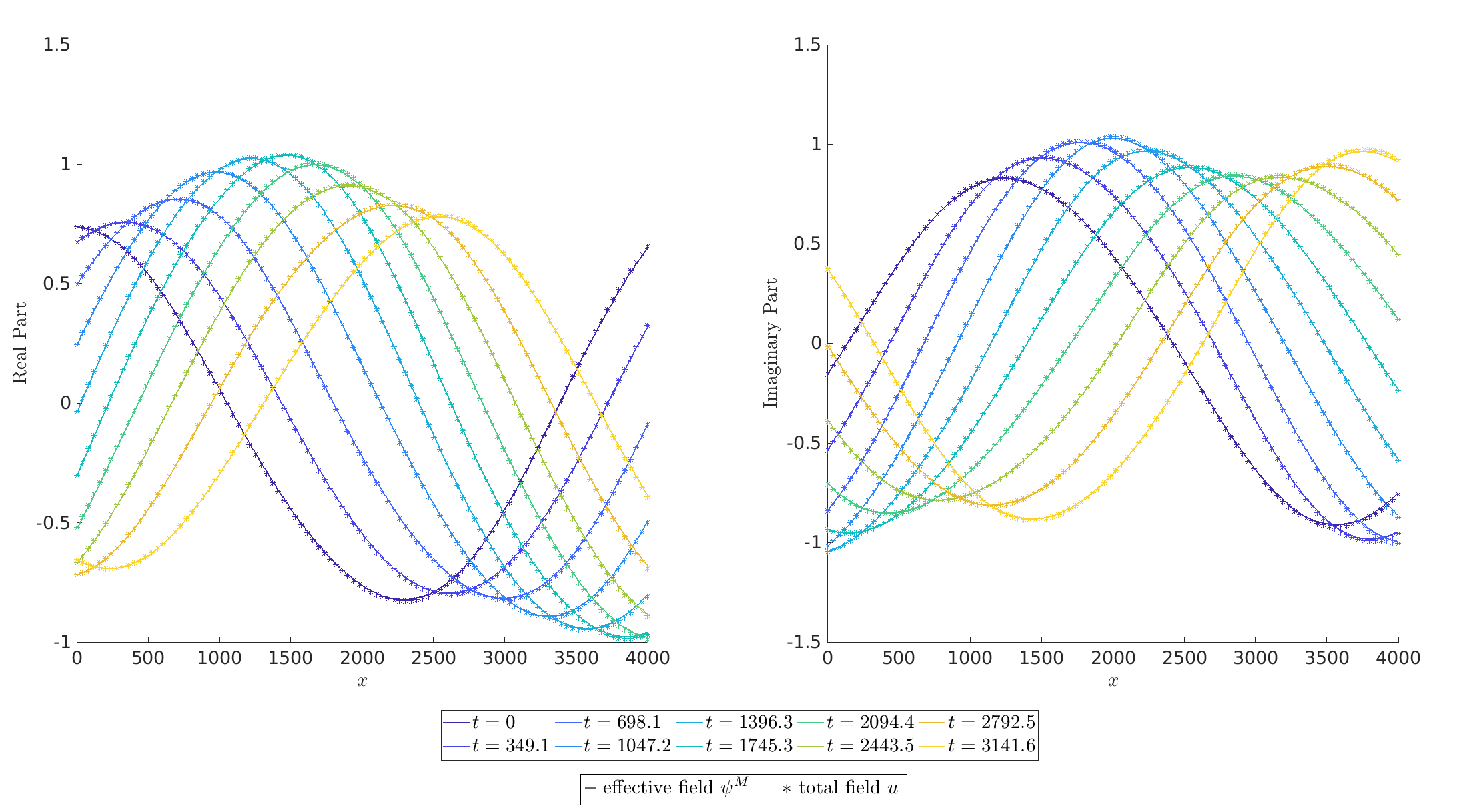
Figure 5.1: The effective field $\psi$ (-) and the total field $u$ (*) plotted next to each other over $\mathcal{U}:=[0,4000]$ with $N=100$ resonators each of length $\ell=0.01$, thus $\Lambda=1$. We set $\gamma=0.05,\,\mu=0.11,\,\xi=0.2,\,K=4,\,\varepsilon_{\kappa}=0.4$. We evaluate the solution at ten time-steps in $[0,T]$, for $T=2\pi/\Omega=3141.59$. For the definition of (5.3) we choose a mesh of size $M=200$.

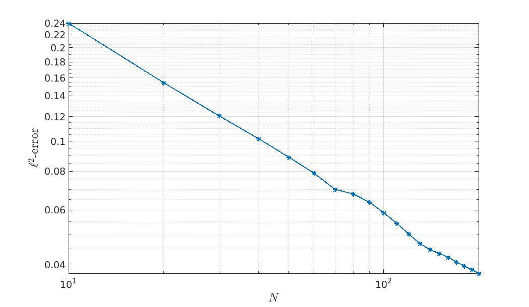
Figure 5.2: The $\ell^{2}$-norm of the error between the effective field $\psi^{M}$ and the total field $u$ at time $t=0$. For the numerical solution we set $M=N$ and $y_{i}=z_{i}$, for convenience. The resonators are evenly distributed inside $\mathcal{U}=[0,4000]$ and each of length $\ell=1/N$. We set $\gamma=0.05,\,\mu=0.11,\,\xi=0.2,\,K=4,\,\varepsilon_{\kappa}=0.4$.

The bold line in Figure 5.1 shows the effective field $\psi^{M}$ as a function of $x$ evaluated at different time-steps inside the interval $[0,T]$. For comparison, we plot the evaluation of the total wave field obtained using the scheme obtained in [2], marked by stars inside the plot. As analytically proved, the effective field and the total field agree for $\ell\ll 1$ and large $N$. The numerical results in Figure 5.1 show that the effective field is still quasi-periodic with quasi-periodicity $\omega$.

Figure 5.2 shows the $\ell^{2}$-norm of the error between the effective field $\psi$ and the true solution $u$ at each resonator $z_{i}$ as a function of $N$. It becomes apparent from our numerical result that the error behaves algebraically in $N$. This result is not surprising, as the effective medium theory only holds in the limit $\ell\to 0$ and $N\to\infty$.

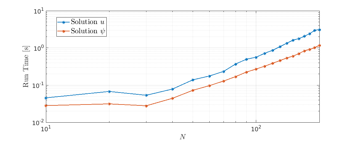
Figure 5.3: The runtime of the computation of $\psi$ solving (5.3) and $u$ solving (2.6). These results correspond to the same setting as in Figure 5.2.

The results in Figure 5.3 show how the computation run time of $u$ is significantly larger than the computation of the effective field $\psi$. This further underlines the relevance of the herein derived effective medium theory.

6 Concluding Remarks

We have rigorously derived an effective medium theory for one-dimensional time-modulated metamaterials in the low-frequency regime. We started by providing the $2\times 2$ scattering matrix for static metamaterials and this led to the point interaction approximation. This set the ground for following a similar approach as in [5]. With suitable assumptions 3.4 - 3.6 we derived the homogenised equation (3.24).

We then proceeded with the case of the time-dependent material parameter $\kappa$. In this paper, we assumed the parameter $\rho$ to be static, since in [1] we proved that the resulting wave field does not depend on $\rho$ at leading order. As in the static case, we first derived the scattering matrix. However, for a time-modulated material parameter, this is a $2(2K+1)\times 2(2K+1)$ matrix. This is a direct consequence of the mode coupling that arises from the modulation in time. Analogously to the static case we then derived a point interaction approximation, which ultimately led to a characterisation of the effective field through a system of coupled Lippmann-Schwinger equations (4.35). These integral equations furnished the homogenised equations given by (4.36). In contrast to the static case, the homogenised equations modelling a time-modulated metamaterial are a system of coupled integro-differential equations.

A crucial assumption to obtain a time-modulated effective medium theory is that the incident frequency $\omega$ is slightly away from the resonant frequency of the components. For a frequency at resonance, the scattering coefficients $g$ are of order one. Even for a large number $N$ of resonators, individual resonator gives a strong contribution to the total field, and the limit does not exist.

Finally, we introduced a numerical scheme to solve the Lippmann-Schwinger equation for the effective field. Our numerical solution supports our analytical results by showing that the numerical solution of (5.3) tends to the numerical solution of (2.6). In fact, Figure 5.2 shows that the error is algebraic in $N$.

We consider the results proven in this paper to be the basis for many new breakthroughs in the exploration of time-modulated metamaterials. Since our results can be easily generalised to higher dimensions, the results herein proved are also of great significance to two- and three-dimensional spacetime metamaterials. Moreover, we showed that time-dependent metamaterials at a resonant frequency cannot be treated as an effective medium.

Code availability

The codes that were used to generate the results presented in this paper are available under https://github.com/rueffl/effective_medium_theory_timedep.

References

- [1] Habib Ammari, Jinghao Cao, Erik Orvehed Hiltunen, and Liora Rueff. Transmission properties of time-dependent one-dimensional metamaterials. J. Math. Phys., 64(12):121502, 12 2023.
- [2] Habib Ammari, Jinghao Cao, Erik Orvehed Hiltunen, and Liora Rueff. Scattering from time-modulated subwavelength resonators. Proc. A., 480(2289):Paper No. 20240177, 22, 2024.
- [3] Habib Ammari, Durga Prasad Challa, Anupam Pal Choudhury, and Mourad Sini. The equivalent media generated by bubbles of high contrasts: Volumetric metamaterials and metasurfaces. Multiscale Modeling & Simulation, 18(1):240–293, 2020.
- [4] Habib Ammari, Erik Orvehed Hiltunen, and Liora Rueff. Space-time wave localisation in systems of subwavelength resonators. Proc. A, to appear, 2025.
- [5] Habib Ammari and Hai Zhang. Effective medium theory for acoustic waves in bubbly fluids near minnaert resonant frequency. SIAM J. Math. Anal., 49(4):3252–3276, 2017.
- [6] Russel E. Caflisch, Michael J. Miksis, George C. Papanicolaou, and Lu Ting. Effective equations for wave propagation in bubbly liquids. Journal of Fluid Mechanics, 153:259–273, 1985.
- [7] Russel E. Caflisch, Michael J. Miksis, George C. Papanicolaou, and Lu Ting. Wave propagation in bubbly liquids at finite volume fraction. Journal of Fluid Mechanics, 160:1–14, 1985.
- [8] Florian Feppon and Habib Ammari. Analysis of a monte-carlo nystrom method. SIAM Journal on Numerical Analysis, 60(3):1226–1250, 2022.
- [9] Florian Feppon and Habib Ammari. Homogenization of sound-soft and high-contrast acoustic metamaterials in subcritical regimes. ESAIM Math. Model. Numer. Anal., 57(2):491–543, 2023.
- [10] R. Figari, G. Papanicolaou, and J. Rubinstein. The point interaction approximation for diffusion in regions with many small holes. In Stochastic methods in biology (Nagoya, 1985), volume 70 of Lecture Notes in Biomath., pages 202–209, 1987.
- [11] R. Figari, G. Papanicolaou, and J. Rubinstein. Remarks on the point interaction approximation. In Hydrodynamic behavior and interacting particle systems (Minneapolis, Minn., 1986), volume 9 of IMA Vol. Math. Appl., pages 45–55. Springer, New York, 1987.
- [12] Leslie L. Foldy. The multiple scattering of waves. i. general theory of isotropic scattering by randomly distributed scatterers. Phys. Rev., 67:107–119, Feb 1945.
- [13] Erik Orvehed Hiltunen and Bryn Davies. Coupled harmonics due to time-modulated point scatterers. Physical Review B, 110(18):184102, 2024.
- [14] P.A. Huidobro, M.G. Silveirinha, E. Galiffi, and J.B. Pendry. Homogenization theory of space-time metamaterials. Phys. Rev. Appl., 16:014044, 2021.
- [15] Steven G. Kargl. Effective medium approach to linear acoustics in bubbly liquids. The Journal of the Acoustical Society of America, 111(1):168–173, 01 2002.
- [16] C. Liu and C. Reina. Dynamic homogenization of resonant elastic metamaterials with space/time modulation. Comput. Mech., 64:147–161, 2019.
- [17] Graeme W. Milton. The theory of composites, volume 88 of Classics in Applied Mathematics. Society for Industrial and Applied Mathematics (SIAM), Philadelphia, PA, 2023.
- [18] C. Rizza, G. Castaldi, and V. Galdi. Nonlocal effects in temporal metamaterials. Nanophotonics, 11(7):1285–1295, 2021.
- [19] Marie Touboul, Bruno Lombard, Raphaël Assier, Sébastien Guenneau, and Richard V Craster. High-order homogenization of the time-modulated wave equation: non-reciprocity for a single varying parameter. Proc. R. Soc. A, 480(2289):20230776, 2024.