Lyapunov Analysis For Monotonically Forward-Backward Accelerated Algorithms
Abstract
In the realm of gradient-based optimization, Nesterov’s accelerated gradient method (NAG) is a landmark advancement, achieving an accelerated convergence rate that outperforms the vanilla gradient descent method for convex function. However, for strongly convex functions, whether NAG converges linearly remains an open question, as noted in the comprehensive review by Chambolle and Pock (2016). This issue, aside from the critical step size, was addressed by Li et al. (2024a) using a high-resolution differential equation framework. Furthermore, Beck (2017, Section 10.7.4) introduced a monotonically convergent variant of NAG, referred to as M-NAG. Despite these developments, the Lyapunov analysis presented in (Li et al., 2024a) cannot be directly extended to M-NAG. In this paper, we propose a modification to the iterative relation by introducing a gradient term, leading to a new gradient-based iterative relation. This adjustment allows for the construction of a novel Lyapunov function that excludes kinetic energy. The linear convergence derived from this Lyapunov function is independent of both the parameters of the strongly convex functions and the step size, yielding a more general and robust result. Notably, we observe that the gradient iterative relation derived from M-NAG is equivalent to that from NAG when the position-velocity relation is applied. However, the Lyapunov analysis does not rely on the position-velocity relation, allowing us to extend the linear convergence to M-NAG. Finally, by utilizing two proximal inequalities, which serve as the proximal counterparts of strongly convex inequalities, we extend the linear convergence to both the fast iterative shrinkage-thresholding algorithm (FISTA) and its monotonic counterpart (M-FISTA).
1 Introduction
Over the past few decades, machine learning has emerged as a major application area for optimization algorithms. A central challenge in this field is unconstrained optimization, which involves minimizing a convex objective function without constraints. Mathematically, this problem is formulated as:
At the heart of addressing this challenge are gradient-based methods, which have driven significant advancements due to their computational efficiency and low memory requirements. These advantages make them particularly well-suited for large-scale machine learning tasks. As a result, gradient-based methods have not only propelled theoretical progress but also facilitated practical breakthroughs, establishing them as indispensable tools in both machine learning research and real-world applications.
One of the simplest and most foundational gradient-based methods is the vanilla gradient descent, which dates back to Cauchy (1847). Given an initial point , the vanilla gradient descent method is implemented recursively as:
where denotes the step size. While this method is effective, it can be slow to converge for convex functions. In the mid-1980s, Nesterov (1983) introduced a two-step accelerated algorithm, now known as Nesterov’s accelerated gradient method (NAG). Given any initial , NAG employs the following update rules:
| (1.1a) | |||
| (1.1b) | |||
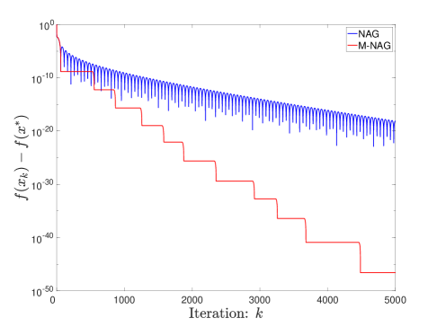
where is the step size, and is the momentum parameter. Compared to the vanilla gradient descent method, NAG achieves accelerated convergence rates. However, it does not guarantee monotone convergence, that is, the function values do not necessarily decrease at every iteration. As a result, oscillations or overshoots may occur, especially as iterates approach the minimizer, as illustrated in Figure 1.
This lack of stability and predictability makes it difficult to monitor progress and ensure reliable convergence. To address this issue, Beck (2017, Section 10.7.4) proposed a variant that achieves both acceleration and monotonicity, referred to as the Monotone Nesterov’s accelerated gradient method (M-NAG). This method incorporates a comparison step to stabilize convergence while maintaining the acceleration properties of NAG. Starting with any initial , the recursive update rules of M-NAG are as follows:
| (1.2a) | |||
| (1.2b) | |||
| (1.2c) | |||
where is the step size and is the momentum parameter. Unlike NAG, M-NAG ensures that the function values are non-increasing at each iteration, thereby providing a more stable convergence path. As illustrated in Figure 1, M-NAG effectively mitigates oscillations while preserving the acceleration characteristic of NAG, leading to more stable and predictable convergence behavior.
A notable advantage of NAG is that it does not require prior knowledge of the modulus of the strong convexity. For strongly convex functions, Li et al. (2024a) utilized the high-resolution differential equation framework (Shi et al., 2022) to establish linear convergence, thereby addressing an open problem posed by Chambolle and Pock (2016). The natural next step is to generalize the Lyapunov analysis proposed in (Li et al., 2024a) from NAG to M-NAG. However, due to the introduction of the comparison step, the phase-space representation that works for NAG cannot be directly applied to M-NAG, making such a generalization quite challenging. This leads to the following question:
1.1 Two key observations
In this paper, we make two key observations for NAG, which allow us to answer the above question through Lyapunov analysis.
1.1.1 Gradient iterative relation
Recall the high-resolution differential equation framework presented in (Chen et al., 2022a; Li et al., 2022b), where Lyapunov analysis based on the implicit-velocity scheme has been shown to outperform the gradient-correction scheme. Accordingly, we adopt the phase-space representation derived from the implicit-velocity scheme. To facilitate this approach, we introduce a new iterative velocity sequence such that . Using this formulation, NAG can be reformulated as follows:
| (1.3a) | |||
| (1.3b) | |||
where the sequence satisfies the following relationship:
| (1.4) |
This phase-space representation allows for a more refined analysis of NAG’s convergence properties. The key idea behind constructing a Lyapunov function, based on the high-resolution differential equation framework (Shi et al., 2022), is the mixed energy, which is derived from the velocity iterative relation. By substituting (1.3a) into (1.3b), we obtain the following iterative relation as
| (1.5) |
where we denote a new iterative sequence , which generate the mixed energy as shown in (Li et al., 2024a). As demonstrated in (Li et al., 2024a), a Lyapunov function is used to derive the linear convergence for NAG. However, due to the existence of kinetic energy, we cannot directly generalize the Lyapunov analysis from NAG to M-NAG.
For convex functions, as shown in (Chen et al., 2022a; Li et al., 2022b), the iterative sequence in (1.5) is used to construct a Lyapunov function, given by:
| (1.6) |
By utilizing the fundamental inequality for strongly convex functions, we can derive the iterative difference satisfying the following inequality:
| (1.7) |
where , , and .111In detail, is the unique global minimum, and the fundamental inequality for strongly convex functions is rigorously shown in (2.3). However, comparing (1.6) and (1.7), it is impossible to align the right-hand side of the inequality (1.7) with the Lyapunov function (1.6) to be proportional, due to the misalignment relationship between the potential energy involving and the mixed energy involving and .
To eliminate the kinetic energy, we introduce a new gradient term, transforming the iteration into a gradient-based iterative form:
| (1.8) |
where the new iterative sequence is given by . The first key observation is this gradient iterative relation (1.8), which enables us to construct a novel Lyapunov function and derive linear convergence. Notably, the convergence rate does not depend on the parameters, except for the momentum parameter , in contrast to(Li et al., 2024a), as detailed in Section 3.
1.1.2 Monotonicity implicitly embedded in NAG
The second key observation pertains to the connection between NAG and M-NAG. By substituting (1.2a) into (1.2c) and reformulating, we derive the following iterative relation:
| (1.9) |
Next, by incorporating the gradient term, we can transform the iterative relation (1.9) into a gradient-based form, yielding:
| (1.10) |
Substituting the position iteration (1.4) into the sequence , we find that the two iterative sequences are identical, i.e., . The detailed calculation is as follows:
Thus, the relationship between the two gradient iterative relations, (1.8) and (1.10), relies solely on the position-velocity relation (1.4). Since the position-velocity relation (1.4) introduces a new iterative sequence , which is free to choose. Hence, the two gradient iterative relations, (1.8) and (1.10), are essentially identical and can be used interchangeably.
With this key observation, we can extend the Lyapunov analysis from NAG to M-NAG. Therefore, it is sufficient to employ Lyapunov analysis to establish the linear convergence for NAG involving the gradient iterative relation (1.10) and the position-velocity relation (1.4), without needing the position iteration (1.3a), as detailed in Section 4.1. This insight reveals that the underlying philosophy of the M-NAG iteration, (1.2a) — (1.2c), is to focus on the iterative sequence to track the monotonicity of function values, while allowing the sequence to adjust correspondingly. In fact, in addition to the freely chosen position-velocity relation (1.4), NAG still consists of two relations: the position iteration (1.3a) and the gradient iterative relation (1.10). With the position-velocity relation (1.4) alone, we cannot directly transform the gradient iterative relation (1.10) into the velocity iteration (1.3b), which still requires the position iteration (1.3a). For M-NAG, we know that it only involves the free-chosen position-velocity relation (1.4) and the gradient iterative relation (1.10).
1.2 Overview of contributions
In this study, building upon the two key observations outlined above, we make the following contributions for the forward-backward accelerated algorithms.
-
(I)
In contrast to the previous work (Li et al., 2024a), we introduce the gradient term to the iterative relation (1.5), resulting in a new gradient-based iterative relation (1.8). This adjustment facilitates the construction of a novel Lyapunov function. Unlike the Lyapunov function developed in (Li et al., 2024a), our new Lyapunov function not only eliminates the kinetic energy, but also guarantees linear convergence for NAG. Moreover, the convergence rate derived from this Lyapunov function is independent of both the parameters of the strongly convex functions and the step size, offering a more general and robust result.
-
(II)
Through some simple substitution, we derive the gradient iterative relation (1.10) for M-NAG. We further observe that this gradient iterative relation (1.10) is equivalent to the one in (1.8) when the position-velocity relation (1.3a) is applied. Additionally, we find that the derivation of linear convergence requires only the gradient iterative relation (1.10), and is independent of the position-velocity relation (1.3a). As a result, we extend the linear convergence from NAG to M-NAG.
-
(III)
Finally, building on the two proximal inequalities for composite functions derived in (Li et al., 2024a, b), which are the proximal counterparts of the two strongly convex inequalities, we extend the linear convergence to the two proximal algorithms, the fast iterative shrinkage-thresholding algorithm (FISTA) and its monotonic counterpart (M-FISTA).
1.3 Related works and organization
In the history of gradient-based optimization algorithms, a significant milestone was the introduction of NAG, a two-step forward-backward algorithm originally proposed by Nesterov (1983). This pioneering work revolutionized optimization techniques by incorporating acceleration into the vanilla gradient descent method, leading to substantial improvements in convergence rates. Building upon this breakthrough, Beck and Teboulle (2009) introduced a proximal version of the fundamental inequality, which paved the way for the development of FISTA. This new algorithm extended the power of NAG to handle composite objective functions, making it a more efficient tool for a wide range of applications, including signal processing and image reconstruction. Further advancing the field, Beck (2017) proposed a monotonically convergent version of the forward-backward accelerated gradient algorithms, ensuring that the algorithm’s performance would steadily improve over time. Simultaneously, adaptive restart strategies were explored to maintain monotonicity and enhance the robustness of forward-backward accelerated algorithms, with some contributions from Giselsson and Boyd (2014) and O’Donoghue and Candes (2015) .
Over the past decade, there has been increasing interest in understanding the acceleration phenomenon in optimization algorithms through the lens of differential equations. This exploration began with works (Attouch et al., 2012, 2014), which sparked a surge of research into the dynamics underlying accelerated methods. The topic gained further prominence with the development of a low-resolution differential equation for modeling NAG (Su et al., 2016), a variational perspective on acceleration (Wibisono et al., 2016), and studies focusing on the faster convergence rate of function values (Attouch and Peypouquet, 2016). The acceleration mechanism was ultimately clarified through comparisons between NAG method with Polyak’s heavy-ball method, with pivotal insights emerging from the high-resolution differential equation framework introduced by Shi et al. (2022). This framework revealed that gradient correction is effectively achieved through an implicit velocity update, providing a more comprehensive understanding of how acceleration arises. Subsequent works (Chen et al., 2022a, b) further demonstrated that this framework is particularly well-suited for NAG. Buildling on this, progress was made by extending the framework to address composite optimization problems, encompassing both convex and strongly convex functions (Li et al., 2022b, a). This extension was achieved by refining the proximal inequality and generalizing the framework to accommodate a wider range of optimization scenarios, including the overdamped case, as shown in (Chen et al., 2023). These advancements have significantly deepened our understanding of acceleration mechanisms and paved the way for more efficient, robust, and versatile optimization algorithms.
The remainder of this paper is organized as follows. Section 2 introduces the foundational definitions and inequalities for strongly convex functions and composite functions, which serve as preliminaries for the analysis. Section 3 outline the construction of the Lyapunov function and establishes the linear convergence for NAG and FISTA. Section 4 extends the linear convergence to the monotonically accelerated forward-backward algorithms, M-NAG and M-FISTA, leveraging the novel Lyapnov function that excludes the kinetic energy. Finally, Section 5 concludes this papers and proposes potential avenues for future research.
2 Preliminaries
In this paper, we adopt the notations that are consistent with those used in (Nesterov, 2018; Shi et al., 2022; Li et al., 2024b), with slight adjustments tailored to the specific context of our analysis. Let denote the class of continuous convex functions defined on . Specifically, if it satisfies the convex condition:
for any and . A subclass of , denoted , consists of functions that are continuously differentiable and have Lipschitz continuous gradients. Specifically, if and its gradient satisfies:
| (2.1) |
for any . Next, we introduce the function class , a subclass of , where each function is -strongly convex for some . Specifically, if and satisfies the -strongly convex condition:
| (2.2) |
for any . For any , the following fundamental inequality can be derived:
| (2.3) |
for any . Additionally, we denote as the unique minimizer of the objective function. Furthermore, for any , we have the following inequality
| (2.4) |
for any .
We now shift focus to a composite function , where and . Building upon the methodologies established in (Beck and Teboulle, 2009; Su et al., 2016), we introduce the concept of the -proximal value, which plays a pivotal role in our analysis.
Definition 2.1 (-proximal value).
Let the step size satisfy . For any and , the -proximal value is defined as
| (2.5) |
for any . The -proximal value in (2.5) minimizes a weighted sum of the squared Euclidean distance between and the gradient-based update , along with the regularization term . The introduction of the -proximal subgradient offers the flexibility to handle composite objective functions, enabling efficient minimization of the form , where may be non-smooth but proximally simple. When is specified as the -norm, i.e., , a closed-form expression for the -proximal value can be derived. Specifically, for any , the -th component of -proximal value is given by:
where and denotes the sign function. This closed-form expression is particularly useful, as it provides an efficient way to compute the -proximal value for the -regularization term, which is widely used in sparse optimization problems.
Definition 2.2 (-proximal subgradient).
For any ., the -proximal subgradient is defined as:
| (2.6) |
where the -proximal value is given by (2.5). The subgradient , as defined in (2.6), captures the direction of improvement for the composite function , based on the -proximal update. It can be viewed as a generalization of the traditional gradient, incorporating the proximal step with respect to the regularizer .
With the definition of -proximal subgradient (2.2), we extend the two key inequalities, (2.3) and (2.4), to the proximal cases. We now present a proximal version of the fundamental inequality (2.3) for a composite function . This result, rigorously established in (Li et al., 2024b), is stated as follows:
Lemma 2.3 (Lemma 4 in (Li et al., 2024b)).
Let be a composite function with and . Then, the following inequality
| (2.7) |
holds for any .
Finally, we present a key inequality for the -proximal subgradient, which will be used in the subsequent sections. This result, previously established in (Li et al., 2024a), is stated as follows:
3 Lyapnov analysis for NAG and FISTA
In this section, we first outline the process of constructing a novel Lyapunov function, following the principled way presented in (Chen et al., 2022b). Specifically, we introduce the iterative sequence in (1.8), which generates the mixed term that plays a pivotal role in the construction of this Lyapunov function.Building on this, we then derive the linear convergence rate for NAG applied to strongly convex functions and formulate a theorem to characterize the result. Finally, we apply Lemma 2.3 and Lemma 2.4 to extend the linear convergence rate to the proximal setting, focusing on the FISTA.
3.1 The construction of a novel Lyapunov function
Following the principled way outlined in (Chen et al., 2022b), we construct a novel Lyapunov function in two main steps: first, by introducing the iterative sequence for the mixed energy, and then by adjusting the coefficient of the potential energy to align with this mixed energy.
-
(1)
Construction of mixed energy Recall the iterative relation (1.8). In the context of convergence analysis, it is not the iterative point itself that matters, but rather its difference from the optimal solution, . To account for this, we introduce a term to both sides of the gradient iterative relation (1.8), yielding:
(3.1) This relation naturally leads to the mixed energy, which is given by:
(3.2) Next, we examine the iterative difference of this mixed energy using the iterative relation (3.1):
(3.3) Substituting (1.4) into (3.3), we derive the following result for the iterative difference:
(3.4) -
(2)
Construction of potential energy In contrast to the Lyapunov function (1.6), previously used for convex functions in (Chen et al., 2022a; Li et al., 2022b), we now modify the potential energy by replacing with . This adjustment aligns the formulation of the potential energy with the mixed energy given in (3.2). Additionally, we introduce a dynamic coefficient to the potential energy, which is expressed as:
(3.5) The iterative difference of this potential energy is then given by:
(3.6) Next, by substituting and into the fundamental inequality (2.3), we obtain the following inequality
(3.7) Substituting (3.7) into the iterative difference (3.6), we derive the following bound on the iterative difference of the potential energy:
(3.8) Substituting (1.3a) into (3.8), we refine the above inequality (3.8) as:
(3.9) To ensure that the term , we choose a dynamica coefficient as .
3.2 Linear convergence of NAG
Using the Lyapunov function (3.10), we can rigorously establish the linear convergence of NAG. The result is formally presented in the following theorem:
Theorem 3.1.
Proof of Theorem 3.1.
We begin by deriving an expression for the change in the Lyapunov function across iterations. By combining the inequalities for the iterative differences, (3.4) and (3.9), we derive the iterative difference for the Lyapunov function (3.10) as follows:
| (3.12) |
Next, by substituting and into the fundamental inequality (2.3) and rearranging, we obtain:
| (3.13) |
Substituting the inequality (3.13) into (3.12), we arrive at the following estimate for the iterative difference as:
| (3.14) |
To further simplify this expression, we use the strongly convex inequality (2.4) to derive the lower bound on as:
| (3.15) |
Substituting this inequality (3.15) into (3.14), we further estimate the iterative difference as
| (3.16) |
Finally, we estimate the Lyapunov function (3.10) using the Cauchy-Schwarz inequality:
| (3.17) |
By comparing the coefficients of the right-hand sides of the two inequalities, (3.12) and (3.17), we deduce the following estimate as:
| (3.18) |
where the last inequality follows from the definition of the integer , and the fact that . Thus, by applying standard inequalities for the gradient Lipschitz condition (2.1), we complete the proof. ∎
3.3 Linear convergence of FISTA
We now extend the linear convergence of NAG, as established in Theorem 3.1, to include its proximal variant, FISTA. As specified in 2.1, FISTA utilizes the -proximal value (2.5) and follows the iterative scheme below, starting from any initial point :
| (3.19a) | |||
| (3.19b) | |||
where denotes the step size. As formulated in 2.2, we can rewrite FISTA using the -proximal subgradient (2.6), resulting in a new iterative scheme similar to NAG as:
| (3.20a) | |||
| (3.20b) | |||
where the -proximal subgradient serves as a natural generalization of the classical gradient used in NAG. This formulation highlights the structural resemblance between M-FISTA and M-NAG, while accounting for the non-smooth nature of . Furthermore, by defining the velocity iterative sequence as , we can express the FISTA updates in a manner akin to NAG, (1.3a) and (1.3b). This leads to the implicit-velocity phase-space representation:
| (3.21a) | |||
| (3.21b) | |||
where the sequence satisfies the following relationship:
| (3.22) |
To derive the linear convergence for FISTA, we still need to establish a suitable Lyapunov function. In this context, we generalize the one (3.10), previously used for smooth functions, as shown in Section 3.2, by replacing the smooth function with the composite function . This modification leads to the following Lyapunov function:
| (3.23) |
As detailed in Section 3.2, the linear convergence for smooth functions predominantly hinges on three key inequalities, (3.7), (3.13), and (3.15). These inequalities serve as the foundation for analyzing the linear convergence of NAG, encapsulating how it approaches the optimal solution. Additionally, Lemma 2.3 and Lemma 2.4 extend the two strongly convex inequalities, (2.3) and (2.4), to the proximal setting. Consequently, we can generalize these three key inequalities, (3.7), (3.13), and (3.15), to account for the proximal components, effectively addressing the challenges posed by the non-smooth components of the objective function. Thus, we can establish the linear convergence for FISTA, as formally stated in the following theorem:
4 Monotonicity and linear convergence
In this section, we extend the linear convergence for NAG and FISTA, as established in Section 3, to their corresponding proximal variants, M-NAG and M-FISTA. Specifically, we use the iterative sequence in the gradient iterative relation (1.10), which only depends on the variables and , rather than the full NAG iterative relations, (1.3a) and (1.10), to construct the Lyapunov function. In deriving the linear convergence, we show that it fundamentally relies on the gradient iterative relation (3.1), specifically, the information from M-NAG, as described in (1.2a) — (1.2c), rather than the full NAG information from (1.1a) and (1.1b). Finally, we generalize the linear convergence to include the proximal variant, M-FISTA.
4.1 Smooth optimization via M-NAG
Using the iterative sequence from the gradient iterative relation (1.10), we write down a new form of the Lyapunov function (3.10), which depnends only on the variables, and , as follows:
| (4.1) |
This form of the Lyapunov function plays a critical role in deriving the linear convergence for M-NAG. The result is rigorously stated in the subsequent theorem.
Theorem 4.1.
Proof of Theorem 4.1.
To calculate the iterative difference of the Lyapunov function, we separate the process into two parts, the potential energy and the mixed energy, as shown in (4.1).
-
(1)
For the potential energy, we calculate its iterative difference as
(4.3) Next, substituting and into the fundamental inequality (2.3) and noting from (1.2b) that , we obtain the following inequality
(4.4) Then, we substitute the inequality (4.4) into the iterative difference (4.3) to derive the following bound as
(4.5) -
(2)
To account for the difference between the iterative point and the optimal solution , we introduce the term to both sides of the gradient iterative relation (1.10). This results in the following iterative relation:
(4.6) Using this modified gradient iterative relation, we can now derive the following expression for the iterative difference of the mixed energy between iterations as:
(4.7) Next, we substitute and into the fundamental inequality (2.3) and rearrange to obtain:
(4.8) Substituting the inequality (4.8) into the iterative difference (4.7) of the mixed energy, we arrive at the following bound:
(4.9)
From the iterative differences of the potential energy and the mixed energy, as described in (4.5) and (4.9), we observe that . This allows us to derive the following bound on the iterative difference:
| (4.10) |
To further simplify this expression, we apply the strongly convex inequality (2.4), which provides a lower bound on as follows:
| (4.11) |
Substituting this bound (3.15) into (4.10), we arrive at the following estimate for the iterative difference:
| (4.12) |
Next, we estimate the Lyapunov function (4.1) using the Cauchy-Schwarz inequality:
| (4.13) |
By comparing the coefficients of the right-hand sides of the two inequalities, (4.12) and (4.13), we deduce the following estimate for the iterative difference:
| (4.14) |
where the last inequality holds due to the definition of the integer and the fact that . Finally, by applying standard inequalities for the gradient Lipschitz condition (2.1), we complete the proof. ∎
4.2 Composite optimization via M-FISTA
We now extend the linear convergence of M-NAG, as established in Theorem 4.1, to include its proximal variant, M-FISTA. As outlined in 2.1, M-FISTA employs the -proximal value defined in (2.5) and follows the iterative scheme below, starting from any initial point :
| (4.15a) | |||
| (4.15b) | |||
| (4.15c) | |||
where denotes the step size. To provide a unified perspective, we introduce M-FISTA, a variant that mirrors the structure of M-NAG. According to 2.2, M-FISTA replaces the -proximal value with the -proximal subgradient, as defined in (2.6). This yields a new iterative scheme that more closely resembles M-NAG, as follows:
| (4.16a) | |||
| (4.16b) | |||
| (4.16c) | |||
where the -proximal subgradient replaces the gradient in NAG.
Similarly, to establish the linear convergence for M-FISTA, we generalize the Lyapunov function (4.1) to its proximal counterpart as follows:
| (4.17) |
In this formulation, we incorporate the proximal structure into the Lyapunov function to account for the non-smoothness of the objective function. Lemma 2.3 and Lemma 2.4 extend the two strongly convex inequalities, (2.3) and (2.4), to the proximal setting. Consequently, we can generalize these three key inequalities, (4.4), (4.8), and (4.11), to o account for the proximal adjustments. With these extensions, we can generalize the linear convergence from M-NAG to M-FISTA, as formally stated in the following theorem:
5 Conclusion and future work
In this paper, we introduce an additional gradient term to the iterative relation (1.5), resulting in a refined gradient-based iterative relation (1.8). This modification paves the way for the development of a novel Lyapunov function. Unlike the Lyapunov function presented in (Li et al., 2024a), our new formulation not only eliminates the kinetic energy but also ensures linear convergence for NAG. Furthermore, the linear convergence derived from this Lyapunov function is independent of both the parameters of the strongly convex functions and the step size, thus providing a more universal and robust result. By performing a series of straightforward substitutions, we derive the gradient-based iterative relation (1.10) for M-NAG. Interestingly, we observe that this gradient iterative relation (1.10) coincides with the one in (1.8) when the position-velocity relation (1.3a) is applied. Additionally, we further demonstrate that the derivation of linear convergence relies solely on the gradient iterative relation (1.10) and does not require the position-velocity relation (1.3a). The key observation allows us to extend the linear convergence from NAG to M-NAG. Finally, leveraging the two proximal inequalities for composite functions developed in (Li et al., 2024a, b), which serves as the proximal analogs of the two classical strongly convex inequalities, we extend the linear convergence to both FISTA) and M-FISTA. This extension broadens the applicability of our results, providing insights into the convergence behavior of these widely used proximal algorithms.
For -strongly convex functions, another Nesterov’s accelerated gradient method, referred to as NAG-SC, was originally proposed by Nesterov (2018). In NAG-SC, the momentum coefficient is defined as , in contrast to used in the standard NAG. The iterative scheme for NAG-SC is given by:
| (5.1a) | |||
| (5.1b) | |||
where is the step size. Building on the same idea introduced by Beck (2017), we can propose a monotonic variant of NAG-SC, which we denote as M-NAG-SC. The iterative scheme for M-NAG-SC is as follows:
| (5.2a) | |||
| (5.2b) | |||
| (5.2c) | |||
where is the step size. We demonstrate the numerical performance of both NAG-SC and M-NAG-SC in comparison with the vanilla gradient descent method in Figure 2.

An intriguing avenue for future research is to explore whether M-NAG-SC, as described by (5.2a) — (5.2c), can retain the accelerated convergence rate of NAG-SC. However, it is important to note that the Lyapunov function presented in (Shi et al., 2022), which incorporates the kinetic energy as an essential part of the analysis, complicates the direct generalization from NAG-SC to M-NAG-SC. Thus, extending the Lyapunov analysis to the monotonic variant requires further exploration.
Acknowledgements
We thank Bowen Li for his helpful and insightful discussions. Mingwei Fu acknowledges partial support from the Loo-Keng Hua Scholarship of CAS. Bin Shi was partially supported by the startup fund from SIMIS and Grant No.YSBR-034 of CAS.
References
- Attouch and Peypouquet [2016] H. Attouch and J. Peypouquet. The rate of convergence of nesterov’s accelerated forward-backward method is actually faster than . SIAM Journal on Optimization, 26(3):1824–1834, 2016.
- Attouch et al. [2012] H. Attouch, P.-E. Maingé, and P. Redont. A second-order differential system with hessian-driven damping; application to non-elastic shock laws. Differential Equations and Applications, 4(1):27–65, 2012.
- Attouch et al. [2014] H. Attouch, J. Peypouquet, and P. Redont. A dynamical approach to an inertial forward-backward algorithm for convex minimization. SIAM Journal on Optimization, 24(1):232–256, 2014.
- Beck [2017] A. Beck. First-order methods in optimization. SIAM, 2017.
- Beck and Teboulle [2009] A. Beck and M. Teboulle. A fast iterative shrinkage-thresholding algorithm for linear inverse problems. SIAM journal on imaging sciences, 2(1):183–202, 2009.
- Cauchy [1847] A. Cauchy. Méthode générale pour la résolution des systemes d’équations simultanées. Comp. Rend. Sci. Paris, 25(1847):536–538, 1847.
- Chambolle and Pock [2016] A. Chambolle and T. Pock. An introduction to continuous optimization for imaging. Acta Numerica, 25:161–319, 2016.
- Chen et al. [2022a] S. Chen, B. Shi, and Y.-x. Yuan. Gradient norm minimization of nesterov acceleration: . arXiv preprint arXiv:2209.08862, 2022a.
- Chen et al. [2022b] S. Chen, B. Shi, and Y.-x. Yuan. Revisiting the acceleration phenomenon via high-resolution differential equations. arXiv preprint arXiv:2212.05700, 2022b.
- Chen et al. [2023] S. Chen, B. Shi, and Y.-x. Yuan. On underdamped nesterov’s acceleration. arXiv preprint arXiv:2304.14642, 2023.
- Giselsson and Boyd [2014] P. Giselsson and S. Boyd. Monotonicity and restart in fast gradient methods. In 53rd IEEE Conference on Decision and Control, pages 5058–5063. IEEE, 2014.
- Li et al. [2022a] B. Li, B. Shi, and Y.-X. Yuan. Linear convergence of ISTA and FISTA. arXiv preprint arXiv:2212.06319, 2022a.
- Li et al. [2022b] B. Li, B. Shi, and Y.-x. Yuan. Proximal subgradient norm minimization of ista and fista. arXiv preprint arXiv:2211.01610, 2022b.
- Li et al. [2024a] B. Li, B. Shi, and Y.-x. Yuan. Linear convergence of forward-backward accelerated algorithms without knowledge of the modulus of strong convexity. SIAM Journal on Optimization, 34(2):2150–2168, 2024a.
- Li et al. [2024b] B. Li, B. Shi, and Y.-X. Yuan. Linear convergence of ISTA and FISTA. Journal of the Operations Research Society of China, pages 1–19, 2024b.
- Nesterov [1983] Y. Nesterov. A method of solving a convex programming problem with convergence rate . Soviet Mathematics-Doklady,, 27(2):372–376, 1983.
- Nesterov [2018] Y. Nesterov. Lectures on Convex Optimization, volume 137. Springer, second edition, 2018.
- O’Donoghue and Candes [2015] B. O’Donoghue and E. Candes. Adaptive restart for accelerated gradient schemes. Foundations of computational mathematics, 15:715–732, 2015.
- Shi et al. [2022] B. Shi, S. S. Du, M. I. Jordan, and W. J. Su. Understanding the acceleration phenomenon via high-resolution differential equations. Mathematical Programming, pages 79–148, 2022.
- Su et al. [2016] W. Su, S. Boyd, and E. J. Candes. A differential equation for modeling nesterov’s accelerated gradient method: Theory and insights. Journal of Machine Learning Research, 17(153):1–43, 2016.
- Wibisono et al. [2016] A. Wibisono, A. C. Wilson, and M. I. Jordan. A variational perspective on accelerated methods in optimization. proceedings of the National Academy of Sciences, 113(47):E7351–E7358, 2016.