Supplementary Materials for Hybrid Data-Free Knowledge Distillation

Table A-1: Details of the benchmark datasets used in our experiment, the items with the prefix “#” denotes the number of the corresponding item.

Dataset	Type	Image size	#classes	#train	#test
CIFAR10	Original data	32$\times$32	10	50,000	10,000
CIFAR100	Original data	32$\times$32	100	50,000	10,000
CINIC	Original data	32$\times$32	10	90,000	90,000
TinyImageNet	Original data	64$\times$64	200	100,000	10,000
HAM	Original data	224$\times$224	7	8,000	2,000
ISIC	Collected data	224$\times$224	8	20,000	5,000
ImageNet	Original&collected data	224$\times$224	1,000	1,281,167	50,000
WebVision	Collected data	224$\times$224	1,000	980,449	N/A

Appendix A Proofs

The Optimal Classifier of Discriminator

For a fixed generator, the optimal classifier $\Psi_{\mathrm{D}}^{*}$ of the discriminator in our employed Auxiliary Discriminative Classifier GAN (ADCGAN) can be formatted as follows:

$$\Psi_{\mathrm{D}}^{*}\left(y^{+}\mid\boldsymbol{x}\right)=\frac{p(\boldsymbol{x},y)}{p(\boldsymbol{x})+q(\boldsymbol{x})},$$ (1)

$$\Psi_{\mathrm{D}}^{*}\left(y^{-}\mid\boldsymbol{x}\right)=\frac{q(\boldsymbol{x},y)}{p(\boldsymbol{x})+q(\boldsymbol{x})}.$$

Proof.

$$\max_{\Psi_{\mathrm{D}}}\mathbb{E}_{\boldsymbol{x},y\sim P_{X,Y}}[\log\Psi_{\mathrm{D}}(y^{+}|\boldsymbol{x})]+$$ (2)

$$\mathbb{E}_{\boldsymbol{x},y\sim Q_{X,Y}}[\log\Psi_{\mathrm{D}}(y^{-}|\boldsymbol{x})]$$

$$\Rightarrow\max_{\Psi_{\mathrm{D}}}\mathbb{E}_{\boldsymbol{x},y\sim P^{m}_{X,Y}}[\log\Psi_{\mathrm{D}}(y|\boldsymbol{x})],$$

with $p^{m}(\boldsymbol{x},y^{+})=\frac{1}{2}p(\boldsymbol{x},y)$, $p^{m}(\boldsymbol{x},y^{-})=\frac{1}{2}q(\boldsymbol{x},y)$, and $p^{m}(\boldsymbol{x})=\sum_{y}p^{m}(\boldsymbol{x},y)=\frac{1}{2}p(\boldsymbol{x})+\frac{1}{2}q(\boldsymbol{x})$. rCl &⇒max_Ψ_DE_x∼P^m_XE_y∼P^m_Y—X[logΨ_D(y—x)]
⇒min_Ψ_DE_x∼P^m_XE_y∼P^m_Y—X[-logΨ_D(y—x)]
⇒min_Ψ_D​​E_x∼​ P^m_X[H(p^m(y—x))​​+​​KL(p^m​(y—x)∥Ψ_D(y—x))]
⇒ Ψ_D^*(y—x)=argmin_Ψ_DKL(p^m(y—x)∥Ψ_D(y—x))
=p^m(y—x)=pm(x,y)pm(x) Therefore, the optimal discriminative classifier of ADC-GAN has the form of $\Psi_{\mathrm{D}}^{*}(y^{+}|\boldsymbol{x})=\frac{p^{m}(\boldsymbol{x},y^{+})}{p^{m}(\boldsymbol{x})}=\frac{p(\boldsymbol{x},y)}{p(\boldsymbol{x})+q(\boldsymbol{x})}$ and $\Psi_{\mathrm{D}}^{*}(y^{-}|\boldsymbol{x})=\frac{p^{m}(\boldsymbol{x},y^{-})}{p^{m}(\boldsymbol{x})}=\frac{q(\boldsymbol{x},y)}{p(\boldsymbol{x})+q(\boldsymbol{x})}$ that conclude the proof. ∎

Proof of Eq. (7)

Given the optimal classifier of the discriminator, at the equilibrium point, encouraging the generator to produce easily classifiable examples of our employed ADCGAN is equivalent to

$$\max_{\mathcal{N}_{\mathrm{G}}}[\mathbb{E}_{\boldsymbol{x},y\sim Q_{X,Y}}[\log\Psi^{*}_{\mathrm{D}}(y^{+}\mid\boldsymbol{x})]$$ (3)

$$-\mathbb{E}_{\boldsymbol{x},y\sim Q_{X,Y}}[\log\Psi^{*}_{\mathrm{D}}(y^{-}\mid\boldsymbol{x})]]$$

$$\Rightarrow\min_{\mathcal{N}_{\mathrm{G}}}\mathrm{KL}\left(Q_{X,Y}\|P_{X,Y}\right),$$

Proof.

rCl &max_N_G E_x,y∼Q_X,Y[logΨ_D^*(y^+—x)]
- E_x,y∼Q_X,Y[logΨ_D^*(y^-—x)]
⇒max_N_G E_x,y∼Q_X,Y[logp(x,y)p(x)+q(x)]
- E_x,y∼Q_X,Y[logq(x,y)p(x)+q(x)]
⇒min_N_GE_x,y∼Q_X,Y[logq(x,y)p(x,y)]
⇒ min_N_G KL(Q_X,Y∥P_X,Y) ∎

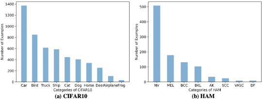
Figure A-1: The number of examples per category in the collected data ($\rho=0.1$), where the original data is (a) CIFAR10 and (b) HAM, respectively.

Algorithm A-1 Hybrid Data-Free Distillation

0:  Pre-trained teacher network $\mathcal{N}_{\mathrm{T}}$, limted collected data $\mathcal{D}_{\mathrm{c}}$.

1:  Initialize the discriminator $\mathcal{N}_{\mathrm{D}}$ and generator $\mathcal{N}_{\mathrm{G}}$ in GAN, and the small student network $\mathcal{N}_{\mathrm{S}}$;

2:  Module 1: Teacher-Guided Generation

3:  repeat

4:     Sample the noise-label pair $(\boldsymbol{z},y)$ to generate synthetic example $\mathcal{N}_{\mathrm{G}}(\boldsymbol{z},y)$;

5:     Mitigate the overfitting of discriminator $\mathcal{N}_{\mathrm{D}}$ via blending $\mathcal{L}_{\mathrm{blend}}$ and transferring $\mathcal{L}_{\mathrm{trans}}$ operations in feature integration;

6:     Calculate the class frequency $\{\hat{n}_{c}\}_{c=1}^{C}$ of synthetic examples;

7:     Regularize the training of generator $\mathcal{N}_{\mathrm{G}}$ across all categories;

8:     Optimize the GAN via Adam;

9:  until convergence

10:  Module 1: Student Distillation

11:  Generate abundant high-quality synthetic examples and inflate collected examples to construct the hybrid data $\mathcal{D}$;

12:  repeat

13:     Sample the example $\boldsymbol{x}\in\mathcal{D}$ and input it into the teacher network $\mathcal{N}_{\mathrm{T}}$ and student network $\mathcal{N}_{\mathrm{S}}$ to obtain the features $\Phi_{\mathrm{T}}(\boldsymbol{x})$ and $\Phi_{\mathrm{S}}(\boldsymbol{x})$, respectively.

14:     Align the features $\Phi_{\mathrm{T}}(\boldsymbol{x})$ and $\Phi_{\mathrm{S}}(\boldsymbol{x})$ via $\mathcal{L}_{\mathrm{align}}$;

15:     Optimize the student network $\mathcal{N}_{\mathrm{S}}$ via SGD;

16:  until convergence

16:  Lightweight student network $\mathcal{N}_{\mathrm{S}}$.

Appendix B Detailed Information of Benchmark Datasets

Comprehensive Dataset Overview

In Table A-1, we introduce the critical information of the benchmark datasets used in our experiment, including the image size, the number of categories, and the number of images in training and test sets. First, we can observe that the large-scale ImageNet contains a large number of examples, when using it as the original data, it is difficult to collect sufficient examples (more than 1 million) from the real-world. Therefore, it is essential to explore an efficient data-free distillation method that requires only a small amount of collected data. Second, a series of benchmark datasets contain 224$\times$224 sized high-resolution images, the generation-based methods that without rely on real-world data are hard to generate high-quality examples to provide effective information for training the student network.

Moreover, Figure A-1 shows the number of collected examples in each category when the original data is the natural image datasets CIFAR10 and practical medical image dataset HAM, respectively. We can observe that the collected examples exhibit imbalanced class distribution, with several categories accounting for the majority of examples and other categories containing only a few examples. Therefore, our proposed data-free distillation method is very practical.

Figure A-2: Visualization of synthetic examples for the original tasks, including (a) CIFAR10, (b) CINIC, (c) TinyImageNet, and (d) HAM.

Visualization of Synthetic Examples

In Figure A-2, we show synthetic examples produced by the GAN trained on limited collected data using our teacher-guided generation module. Specifically, we generate synthetic instances for four original datasets, including CIFAR10, CINIC, TinyImageNet, and HAM. Despite these original datasets having significantly different image sizes (ranging from 32$\times$32 to 224$\times$224), the corresponding synthetic examples consistently exhibit high quality. These visual results demonstrate the effectiveness of our approach in leveraging the teacher network to address critical issues of GAN training on limited collected data. By doing so, our method can train reliable student networks on abundant high-quality synthetic examples.

Appendix C Algorithm

The detailed training algorithm of our proposed HiDFD is summarized in Algorithm A-1. Our HiDFD contains two primary modules to train a reliable student network only using a small number of collected examples, i.e., the teacher-guided generation and student distillation. In the teacher-guided generation, the GAN is trained on the limited collected data under the guidance of the teacher network, where the critical issues, i.e., overfitting of the discriminator and imbalanced learning of the generator, are effectively resolved. In the student network, the collected examples are properly inflated via repeating and combined with sufficient high-quality synthetic examples to construct the hybrid data. Then, the reliable student network can naturally train on the hybrid data via the effective classifier-sharing-based feature alignment strategy.

Appendix D Limitations and Broader Impacts

Limitations

The proposed method can train reliable student networks using very few collected examples. Compared with previous methods, we have reduced the data requirement by 99%, making our method suitable for practical applications. In general, the effectiveness of the proposed method depends on the quality and representativeness of collected data to some extent. If this collected data does not sufficiently represent the broader dataset or contains biases, the generated synthetic examples and the trained student network may inherit these flaws. In practice, collecting fewer representative examples in real-world applications is relatively easy. Therefore, we believe that these limitations can be overcome well.

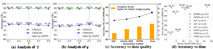
Figure A-3: Parametric sensitivities of (a) $\gamma$ in Eq. (12) and (b) $q$ in Eq. (9). Accuracies (in %) of the student networks trained with (c) synthetic examples generated by various generative models. (d) shows the accuracies and training times of various DFKD methods.

Broader Impacts

This paper proposed a novel data-free knowledge distillation method called HiDFD, which can train a compact and reliable student network using very few collected examples. In general, the proposed HiDFD could have the following positive impacts: 1) HiDFD eliminates the need for original training data required by traditional knowledge distillation methods, so it can help preserve data privacy for users; 2) HiDFD effectively compresses the large pre-trained models (i.e., the teacher networks) into smaller and faster models (i.e., the student networks) that are resource-efficient and suitable for deployment on devices with limited capabilities; 3) HiDFD focuses on the classification tasks, which underpin many practical downstream tasks like object detection and segmentation, suggesting its wide applicability; and 4) HiDFD is compatible with different DNNs (e.g., ResNet and VGG).

Although HiDFD has few negative social impacts, when it compresses the large models of many Artificial Intelligence (AI) technologies and enables these compressed models in practical applications, the proposed HiDFD can be used for good and also for harm, depending on human intent. This actually falls into the general ethical debate on whether AI is good or not.

In conclusion, we believe our proposed work can be beneficial to society since many important real-world applications need compact and reliable models that stand to benefit from HiDFD when the available real-world data is limited.

Appendix E Additional Experiments

Additional Parametric Sensitivities

There are also two tuning parameters $q$ and $\gamma$ in Eq. (9) and $\gamma$ in Eq. (12), respectively. To analyze their sensitivities, we individually vary each parameter while keeping the others constant during training. The accuracies of the corresponding student networks are shown in Figure A-3. Despite the large fluctuations in these parameters, where $q$, $\gamma\in$ {0.1, 0.3, 0.5, 0.7, 0.9}, the accuracy curve of the student network remains relatively stable. These results indicate the robustness of our HiDFD against parameter variations. Additionally, the student network achieved the best performance when $q=0.7$ and $\gamma=0.5$, so we adopted such parameter configuration in our method.

Experiments on Various Collected Data

We compare the quality of synthetic examples produced by different generative models trained with the limited collected data and report the accuracies of the corresponding student networks in Figure A-3(c). Here, the higher-quality synthetic data consistently promotes a better student network, which demonstrates that improving the quality of synthetic examples can effectively improve the performance of the student network.

Moreover, we compared the training time of our method with other collection-based DFKD methods, as depicted in Figure A-3(d). We can observe that our method can train a student network with satisfactory performance within a few hours on an A100 GPU. These results further demonstrate the effectiveness of our HiDFD in training reliable student networks leveraging limited collected data.