Surface Wave-Aerodynamic Roughness Length Model for Air-Sea Interactions
Abstract
A recently introduced model to evaluate the equivalent hydrodynamic length scale for turbulent flow over static rough surfaces is reformulated and extended to enable evaluation of for moving surface waves. The proposed Surface Wave-Aerodynamic Roughness Length model is based on maps of the surface height and its vertical speed as function of position, and Reynolds number. Pressure drag is estimated by approximating the local flow as ideal inviscid ramp flow [Ayala \BOthers. (\APACyear2024)]. Wave history effects are included through dependence on the local velocity difference between the air and wave speed. The model is applied to monochromatic and multiscale surfaces, and the predicted surface roughness length scales are compared to measured values and to commonly used wave parametrization methods found in the literature. The proposed model shows significantly improved agreement with data compared to other models.
Geophysical Research Letters
Department of Mechanical Engineering, Johns Hopkins University, Baltimore, USA \correspondingauthorManuel Ayalamayala5@jhu.edu
Introduces a fluid mechanics-inspired surface roughness model for turbulent flow over moving ocean waves using wave height distribution maps
Validates the model predictions against experimental and simulation data, results show improved accuracy over traditional empirical models.
Casts results in terms of the familiar Charnock coefficient that can now incorporate
Plain Language Summary
This paper introduces a new method to predict the surface drag force imposed on wind blowing over ocean surface waves. Drag prediction methods are needed for weather prediction, climate modeling, and to support engineering tasks e.g., in offshore wind energy applications. The drag force is typically parameterized using a length-scale called the roughness scale; a measure of the resistance to the wind at the wind-wave interface due to moving surface waves. Traditional methods to evaluate this roughness scale rely on data-fitting or assumptions that often do not sufficiently capture the underlying physics. This study introduces a new physics-based approach that predicts the roughness scale based on geometric knowledge about the moving surface. The model is tested on simple and complex wave shapes. Predictions show agreement with data that is significantly better than traditional methods. The model can help improve simulations used for weather forecasting, hurricane prediction, climate modeling, and offshore wind farm design.
1 Introduction
Accurate prediction of the fluxes between the air and sea is essential for advancing weather forecasting, climate studies [Cronin \BOthers. (\APACyear2019)], and offshore wind energy [Veers \BOthers. (\APACyear2023)]. However, developing accurate and practical parameterizations of air-sea surface fluxes remains challenging due to the inherent complexity of atmospheric boundary layer (ABL) turbulence. Similar to static surface roughness, moving waves play a critical role in shaping the momentum balance between turbulent flows and underlying surfaces [Sullivan \BBA McWilliams (\APACyear2010), Chung \BOthers. (\APACyear2021)]. However, unlike static roughness elements that are fixed, wave fields move, and are characterized by local phase and orbital velocities that affect the air flow above. Nonetheless, flow over both surfaces often result in logarithmic (or Monin-Obukov similarty theory based) profiles of the mean air velocity, at sufficiently high Reynolds number. Therefore, the averaged wave effects can be similarly represented with an equivalent hydrodynamic length scale, [Deskos \BOthers. (\APACyear2021)]. Determining this scale based on information about the surface without having to perform costly experiments or eddy-resolving numerical simulations remains an open question.
In the case of static surface roughness, determination of utilizes topographical parameters that depend solely on the geometry of the surface [Chung \BOthers. (\APACyear2021)]. Approaches for estimating equivalent roughness length scales a priori have been developed with some success using empirical fit models [Flack \BBA Chung (\APACyear2022)], machine learning approaches [Aghaei Jouybari \BOthers. (\APACyear2021)], and more recently, a fluid mechanics-based geometric parameter called the wind-shade factor [Meneveau \BOthers. (\APACyear2024)]. On the other hand, due to the inherently time-varying nature of waves, most approaches for determining equivalent surface roughness for surface waves rely heavily on empirical fits to available data [Deskos \BOthers. (\APACyear2021)]. Several widely used parameterizations include the Charnock model [Charnock (\APACyear1955)], the Donelan model [Donelan (\APACyear1990)], the Taylor model [Taylor \BBA Yelland (\APACyear2001)], and the Drennan model [Drennan \BOthers. (\APACyear2003)]. The Charnock model relates roughness length to wind stress, while the Donelan and Drennan models focus on wave age and amplitude. The Taylor model emphasizes wave steepness instead of wave age. For a more comprehensive discussion of these and other models, we refer to [Zhao \BBA Li (\APACyear2024)]. Mesoscale simulations of offshore wind farms [Jiménez \BOthers. (\APACyear2015)] and hurricane modeling [Davis \BOthers. (\APACyear2008)] employ such models within the Weather Research and Forecasting (WRF) framework. Global climate models also use such parameterizations to represent surface fluxes [Couvelard \BOthers. (\APACyear2020)]. Similarly, Large Eddy Simulations (LES) of microscale meteorological boundary layers using WRF-LES [Muñoz-Esparza \BOthers. (\APACyear2014), Ning \BOthers. (\APACyear2023)] or LES of offshore wind turbine flows [Johlas \BOthers. (\APACyear2020), H. Yang, Ge, Abkar\BCBL \BBA Yang (\APACyear2022)] have used -models to capture wave-induced effects. While existing models for have yielded useful results, they often lack robustness across diverse wave conditions [Cronin \BOthers. (\APACyear2019)], motivating the search for more universal models that can generalize across varying wave fields while reducing reliance on tuning coefficients.
In this Letter we describe a new method to determine for a given moving wave-field. The proposed Surface Wave-Aerodynamic Roughness Length (SWARL) model uses a physics-based approach that requires only maps of a wave field’s spatial distribution of surface heights at two successive times, and the relevant Reynolds number as inputs. A scalar parameter, , is then evaluated numerically (or analytically when possible) as a surface average of geometric surface properties. An iterative procedure is used to capture dependence on wave age and Reynolds number. The proposed model is validated against data and existing models for monochromatic and multiscale waves.
2 Surface Wave-Aerodynamic roughness length model
We begin by expressing the momentum exchange (total drag force on planform area ) as an integral of a surface stress, , according to , where is the friction velocity. The wall stress consists of two contributions: pressure (form drag) , and viscous and small-scale roughness drag , the latter from surface features smaller than the resolved ones causing pressure stress.
The pressure stress is modeled using the wall stress model for moving surfaces introduced in \citeAayala2024, in which wave-resolving effects are included through an LES boundary condition rather than a wave-phase adapting computational grid. The model assumes that in the frame of the wave’s local phase speed with incoming relative velocity (where is the air velocity at some reference height above the wave mean elevation), the local flow can be represented as potential flow over a ramp with slope angle . The average pressure over such a ramp is proportional to the relative velocity squared and and the pressure contribution (form drag) to the modeled stress can be written as
| (1) |
Here is the known surface height distribution as function of horizontal positions and time , , and is the local phase-velocity of the wave, i.e., the horizontal speed of the surface’s local vertical projection can be computed from [Ayala \BOthers. (\APACyear2024)], as
| (2) |
(Note that there are points for which , diverges, since is in the denominator of (2), but at any of these points and , so there are no singularities when evaluating .) The local surface unit normal in the horizontal plane is given by (i=1,2). In \citeAayala2024 it was assumed that displacement of the streamlines causes a pressure drop or prevents pressure recovery on the leeside of the wave, such that the pressure force there can be neglected. So, the Heaviside function is used to impose the pressure force only on the faceward side of the wave.
Instead of following \citeAayala2024 in which the reference velocity was taken at a vertical distance equal to the horizontal LES grid spacing , we assume the reference velocity is a constant representing the mean air velocity at a height , some sufficiently far fixed distance above the wave field. Following \citeAmeneveau2024 is set to a multiple of the roughness (wave) amplitude. Since the mean velocity reference is assumed constant, without loss of generality we may align the axis with this mean air velocity (i.e. ). Then, realizing that and are in the same direction, we can expand equation 1, rearrange and simplify to obtain the resulting kinematic wall stress in the -direction:
| (3) |
where the subscript denotes normalization with friction velocity . To model , i.e., tangential viscous stress contributions as well as unresolved surface form drag effects, we use a friction factor model:
| (4) |
The friction factor can be determined using the generalized Moody diagram fit [Meneveau (\APACyear2020)], that depends on
| (5) |
Here is the smooth surface friction coefficient which has been fitted to results from numerical integration of the equilibrium model differential equation [Meneveau (\APACyear2020)]. The fit in it’s simplest form (as also used in \citeAmeneveau2024) is given by , where is the von Karman constant. Moreover, so for any given it can be computed knowing the height and fluid viscosity . The second term in Eq. (5) represents the effects of unresolved small-scale sea surface features such as capillary waves that cannot be evaluated numerically on the surface discretization grid. The drag from these unresolved surface features is included by means of a small-scale roughness length . This length can be expressed in terms of the root-mean-square surface fluctuations below the resolution with which is known, using the result from \citeAGeva:
| (6) |
where is the root mean square of the sub-grid surface height distribution. The -dependent term in Eq. (5) vanishes for surfaces that are known to be smooth below the resolved elevation field ().
The total horizontal drag is given by
| (7) |
where, similarly to the definition of the “wind-shade factor” of \citeAmeneveau2024, we define the factor implicitly according to
| (8) |
where and we have used so that . The slope , angle , local surface normal vector , and local phase speeds are all quantities that depend on position () and time. If the area is large enough, the planar averaging over , denoted by brackets , is expected to converge to a well defined value of even for a single snapshot of a realization of the wave field (however, note that to determine the vertical surface speed is also required). Solving for requires averaging over a known surface elevation map numerically (except for some monochromatic waves, as discussed below). For a given value of (or ) obtained during an iteration step from Eq. (8), the roughness length can be determined from , leading to:
| (9) |
The reference height is chosen following \citeAmeneveau2024, as , where the typical dominant positive height of the surface is defined and computed as where is the surface elevation relative to the mean. This dominant height, , approximately represents the maximum positive deviation above the mean surface height and is closely related to typical characteristic wave heights, such as the significant wave height . The choice of ensures a consistent measure of the “typical” or representative maximum positive wave height across different wave conditions.
If the friction Reynolds number is imposed (as is often the case in numerical simulations), for a known boundary layer hight and air viscosity , the value of can be specified a priori. Since for a given surface the local phase speed can be determined locally at each point, the dimensionless value can be evaluated at each point of the surface and used in the evaluation of . (For numerical convenience we clip the phase velocity when tends to zero in Eq. 2 to , where m/s. Using ensures that the cutoff corresponds to speeds significantly faster than the fastest expected waves, of a size the most dominant wavelength.) In many cases, however, may not be known a priori but instead we may know the air velocity at some reference height (e.g., the common choice m). In that case we may start with some initial guess for , evaluate using Eq. (8), then evaluate . With a new value for thus determined, a next value of is computed, using Eq. (8). Once converged, the final value of is determined using Eq. (9).
3 Results
We apply the proposed model to several cases with known full surface distribution and specified turbulent friction Reynolds number (or friction velocity ) or some reference air velocity. For the iterative procedure to determine and , we use a Newton-Rahpson method to obtain a converged solution of Eq. (8) using a tolerance of .
For monochromatic waves of the form with small values, the calculation of can be simplified: With and , , constant everywhere, and a spatially constant wave-history term . Noting that the average of over half wavelength (since only the forward-facing side generates drag as discussed above) is , we obtain:
| (10) |
Note that the simplified model is expected to lose validity for wave steepness greater than about ( degrees) because of the small angle approximation . For more realistic multiscale wavefields such as ocean waves with a known spectrum, realizations of the wave height can be generated by the usual method of superposing random-phase traveling waves with a prescribed surface spectrum such as the JONSWAP spectrum [K. Hasselmann \BOthers. (\APACyear1973)], a spreading function , and a dispersion relation .
Table 1 shows the series of monochromatic and multiscale wave field cases the model is applied to. For both wave types, we select cases that have been previously studied in high-resolution experiments [Buckley \BOthers. (\APACyear2020), Yousefi \BOthers. (\APACyear2020)], wave-resolved simulations [Wang \BOthers. (\APACyear2021), Hao \BOthers. (\APACyear2021), Zhang \BOthers. (\APACyear2019), Cao \BBA Shen (\APACyear2021), D. Yang \BOthers. (\APACyear2013)] and experimental field campaigns [Drennan \BOthers. (\APACyear2003), Janssen (\APACyear1997), Romero \BBA Melville (\APACyear2010), Johnson \BOthers. (\APACyear1998)]. The wind and wave were aligned in the multiscale wave cases from the field campaigns.
Since typically only the peak wavenumber () was reported, we generate the multiscale surface utilizing a standard default wave spectrum model. The \citeAjanssen1997,johnson_1998 cases reported using the Pierson-Moskowitz (P-M) model [Pierson Jr. \BBA Moskowitz (\APACyear1964)] to characterize their wave spectrum, therefore we also use the P-M model to generate surfaces for these cases:
| (11) |
where is the Phillips constant. We prescribe some directionality by adopting a widely used spreading function [D\BPBIE. Hasselmann \BOthers. (\APACyear1980), Cartwright (\APACyear1963)] if , where . For cases where no spectrum model was mentioned in the prior studies, we use the JONSWAP spectrum:
| (12) |
where , is a parameter and the same is used. Since the Phillips parameter was not reported in the field campaign cases, we use as given by [Donelan \BOthers. (\APACyear1985)], where is the velocity measured at 10 m height. Since using conventional grid resolutions to generate the surface will make the surface inherently filtered at the grid resolution, we include drag effects of the sub-filter features using equation 6.
The r.m.s of the sub-filter features () is evaluated by integrating the one-dimensional form of Eq. (11) from to infinity, resulting in:
| (13) |
The monochromatic wave cases were generated using as the surface. While for many of these cases the simplified expression Eq. (10) could be used, in some cases the wave steepness exceeded 0.28. So, for procedural consistency and testing purposes, all wave surfaces were generated numerically. The numerically generated surfaces used a grid with domain size . Two successive times separated by a small sec were stored. A grid-dependence study using the current methodology found no significant changes in the results using finer grid resolutions. Spatial and temporal gradients of all surfaces were computed using simple first-order finite differencing. None of the wave cases examined in this study exceeded the swell condition of . A study of the model’s applicability for swell conditions and further modification of the model to include these effects is left for future work.
| Case | Symbol | ||||||
|---|---|---|---|---|---|---|---|
| W1 | - | (0.10) | 2.00 | 0.11 | 11.6 | 6.4 | |
| H1 | - | (0.14) | 19.3 | 0.50 | 10.6 | 10.0 | |
| H2 | - | (0.14) | 7.70 | 0.50 | 9.54 | 3.66 | |
| Z1 | - | (0.10) | 7.25 | 0.11 | 4.96 | 2.61 | |
| Z2 | - | (0.10) | 23.8 | 0.11 | 2.97 | 1.73 | |
| B1 | - | (0.06) | 6.57 | 0.13 | 28.8 | 28.9 | |
| B2 | - | (0.12) | 3.91 | 0.30 | 9.00 | 3.80 | |
| B3 | - | (0.17) | 2.62 | 0.58 | 3.82 | 3.72 | |
| B4 | - | (0.20) | 1.80 | 0.99 | 9.20 | 5.00 | |
| B5 | - | (0.26) | 1.53 | 1.04 | 14.8 | 12.3 | |
| C1 | - | (0.15) | 3.46 | 0.04 | 52.4 | 22.2 | |
| C2 | - | (0.15) | 15.4 | 0.04 | 8.40 | 17.5 | |
| Y1 | 19.0 | 0.28 | 10.0 | 33.0 | 3.60 | 4.38 | |
| Y2 | 13.0 | 0.20 | 18.0 | 33.0 | 3.30 | 2.73 | |
| D1 | 7.06 | 0.20 | 14.7 | 397 | 0.235 | 0.391 | |
| D2 | 7.81 | 0.26 | 21.4 | 280 | 0.105 | 0.264 | |
| D3 | 8.04 | 0.24 | 15.7 | 410 | 0.183 | 0.362 | |
| D4 | 6.14 | 0.17 | 24.0 | 162 | 0.093 | 0.328 | |
| J1 | 7.20 | 0.22 | 17.8 | 371 | 0.336 | 0.275 | |
| J2 | 7.75 | 0.34 | 12.5 | 581 | 0.330 | 0.247 | |
| J3 | 7.83 | 0.30 | 13.0 | 581 | 0.402 | 0.277 | |
| J4 | 7.40 | 0.25 | 14.5 | 432 | 0.332 | 0.298 | |
| R1 | 10.9 | 0.25 | 8.20 | 498 | 0.637 | 1.02 | |
| R2 | 6.24 | 0.21 | 23.6 | 381 | 0.101 | 0.206 | |
| R3 | 7.96 | 0.22 | 15.0 | 465 | 0.172 | 0.405 | |
| R4 | 8.46 | 0.18 | 14.9 | 344 | 0.134 | 0.560 | |
| S1 | 6.85 | 0.17 | 19.1 | 113 | 0.687 | 0.523 | |
| S2 | 8.02 | 0.21 | 13.2 | 187 | 0.382 | 0.606 | |
| S3 | 9.77 | 0.25 | 10.1 | 293 | 0.572 | 0.648 | |
| S4 | 11.2 | 0.29 | 8.50 | 346 | 0.744 | 0.336 |
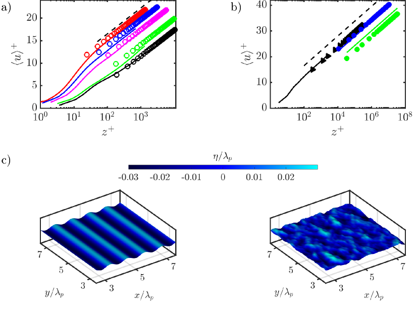
We first focus on the logarithmic mean wind velocity profiles above the wave field for some representative cases of monochromatic and multiscale wave fields. Figure 1a shows measured mean velocity profiles from a laboratory experiment [Buckley \BOthers. (\APACyear2020), Yousefi \BOthers. (\APACyear2020)] (lines) and corresponding logarithmic profile with the values of as determined using the SWARL model (symbols). Figure 1b shows a similar comparison for multiscale wave fields based on cases Y1, S1 and S4. Realizations of surface elevation maps for cases B3 and Y1 are shown in figure 1c. The results demonstrate good agreement between the model predictions and the reference data.
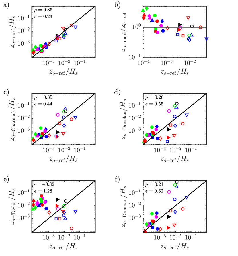
For a more complete comparison of the model’s predictive strength, figure 2a and 2b show scatter plots of modeled surface roughness versus reference data. The surface roughness from the reference cases are either provided or are obtained by taking the reference velocity profiles and fitting the log law region with a least square method. For some of the experimental cases, the surface roughness was estimated using , where is 10 m and . For all wave types, there is good overall agreement between the predicted and measured values. The correlation coefficient for our model is about 85% and we also estimate the average logarithmic error magnitude to be around .
Next, we compare to several commonly used -parameterizations in the literature. The Charnock model remains the most widely used parameterization for air-sea momentum transfer, with applications in fields such as hurricane modeling [Davis \BOthers. (\APACyear2008)] and offshore wind energy [Johlas \BOthers. (\APACyear2020), H. Yang, Ge, Gu\BCBL \BOthers. (\APACyear2022)]. It is expressed as:
| (14) |
where is the phase speed of the peak wave, and is the Charnock coefficient. This coefficient is reported to vary between 0.011 and 0.035, [Deskos \BOthers. (\APACyear2021)]. For the comparison we use , which reflects the center of the reported range. We also provide comparisons with the Donelan model [Donelan (\APACyear1990)]: , the Taylor-Yelland model [Taylor \BBA Yelland (\APACyear2001)]: , and the Drennan model [Drennan \BOthers. (\APACyear2003)]: . The corresponding scatter plots and the correlation coefficients and logarithmic errors are shown in figure 2c-f. Here, the Charnock model shows the strongest overall correlation with observations with a correlation coefficient of 37%. However, as discussed above the proposed SWARL model significantly exceeds this accuracy, yielding a correlation coefficient of , i.e., more than twice that of the Charnock model.
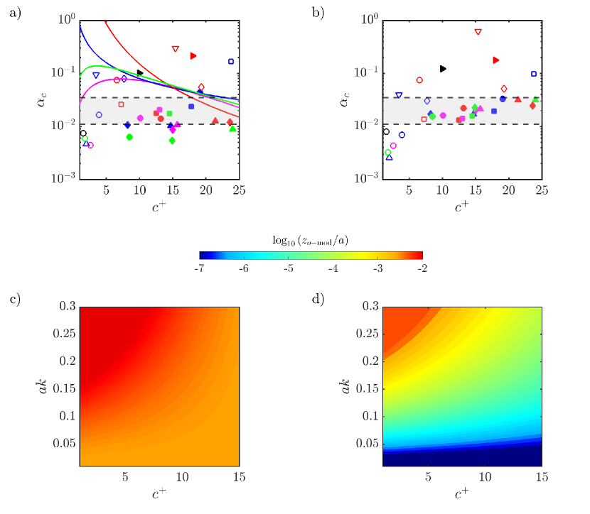
In order to cast the comparison in terms of another common parameter, we also present results in terms of the effective (modified) Charnock coefficient:
| (15) |
where the last equality is for the proposed model when is expressed in terms of and . Although numerous formulations exist for , each parameterized by wave properties, no universal formulation has been established. Most are derived from data fitting [Zhao \BBA Li (\APACyear2024), Lin \BBA Sheng (\APACyear2020)]. The modified Charnock coefficient was calculated for all wave cases shown in Table 1 and the results from data (using the measured values of ) are plotted in figure 3a alongside results from the SWARL model using the same symbols in figure 3b. For comparison, four distinct formulations of the Charnock coefficient, all based solely on wave age (), are also shown as lines, which show poor agreement with the scattered data. In contrast, the values of the modified Charnock coefficient derived from the proposed model show the desired lack of one-to-one dependence or single scaling with wave age. Rather, the model incorporates dependency on additional parameters beyond wave age, namely wave steepness (capturing surface geometric effects) and wind conditions (via ).
Focusing on the case of monochromatic waves, the simplified model from Eq. (10) enables us to perform a broad parametric study over a range of flow parameters (mainly ) and wave parameters ( and ). Figures 3c,d, show contour plots of the modeled surface roughness for a range of wave parameters at and . The results show that for the low , is proportionally a larger fraction of as compared to the high case, and further confirm dependence of on multiple parameters, i.e., , , and .
4 Conclusions
This study introduces a surface roughness model for turbulent flow over moving ocean waves. Unlike traditional models that rely on small subsets of relevant parameters and empirical parameter tuning, the proposed model includes dependence on full geometric characteristics of the wave surface, offering more general applicability. For multiscale surfaces, discretized realizations of wave-height fields at two consecutive times are needed. For monochromatic and small amplitude waves, a simplified formulation is derived that enables prediction using only simple wave parameters such as amplitude, wavelength and phase speed. This simplified approach is particularly useful for parametric studies. We express the proposed model in terms of a modified Charnock coefficient that offers a more comprehensive representation of air-sea momentum exchange.
The model’s performance is validated against monochromatic and multiscale wave fields, showing good agreement with experimental and simulation-based reference data. Comparisons with widely used empirical models demonstrate the superior accuracy and broader applicability of the proposed method across diverse wave conditions. The approach can thus enhance atmospheric boundary layer simulations in mesoscale and micro-mesoscale modeling frameworks, such as WRF-LES. Additionally, we envision that with in-situ measurements of wave height and wind velocity, the proposed model could provide an efficient means of determining surface momentum flux () from wave surface measurements, offering practical utility in interpreting field data. Future work extending the model to account for the dynamics of swell conditions, wave breaking, modeling scalar fluxes, are fruitful future challenges beyond the scope of this study.
Open Research Section
Data files and Matlab code to compute the roughness scale can be downloaded from the repository at https://github.com/ayalamanuel/SWARL
Acknowledgements.
This work was supported by the National Science Foundation and the Department of Energy (via NSF grant CBET-2401013) and by the U.S. Department of Energy, Office of Science Energy Earthshot Initiative, as part of the Addressing Challenges in Energy—Floating Wind in a Changing Climate (ACE-FWICC) Energy Earthshot Research Center.References
- Aghaei Jouybari \BOthers. (\APACyear2021) \APACinsertmetastarAghaeiJouybari2021{APACrefauthors}Aghaei Jouybari, M., Yuan, J., Brereton, G\BPBIJ.\BCBL \BBA Murillo, M\BPBIS. \APACrefYearMonthDay2021. \BBOQ\APACrefatitleData-driven prediction of the equivalent sand-grain height in rough-wall turbulent flows Data-driven prediction of the equivalent sand-grain height in rough-wall turbulent flows.\BBCQ \APACjournalVolNumPagesJournal of Fluid Mechanics912A8. {APACrefDOI} 10.1017/jfm.2020.1085 \PrintBackRefs\CurrentBib
- Ayala \BOthers. (\APACyear2024) \APACinsertmetastarayala2024{APACrefauthors}Ayala, M., Sadek, Z., Ferčák, O., Cal, R\BPBIB., Gayme, D\BPBIF.\BCBL \BBA Meneveau, C. \APACrefYearMonthDay2024. \BBOQ\APACrefatitleA Moving Surface Drag Model for LES of Wind Over Waves A moving surface drag model for les of wind over waves.\BBCQ \APACjournalVolNumPagesBoundary-Layer Meteorology1901039. \PrintBackRefs\CurrentBib
- Buckley \BOthers. (\APACyear2020) \APACinsertmetastarbuckley2020{APACrefauthors}Buckley, M\BPBIP., Veron, F.\BCBL \BBA Yousefi, K. \APACrefYearMonthDay2020. \BBOQ\APACrefatitleSurface viscous stress over wind-driven waves with intermittent airflow separation Surface viscous stress over wind-driven waves with intermittent airflow separation.\BBCQ \APACjournalVolNumPagesJournal of Fluid Mechanics905A31. {APACrefDOI} 10.1017/jfm.2020.760 \PrintBackRefs\CurrentBib
- Cao \BBA Shen (\APACyear2021) \APACinsertmetastarcao_shen_2021{APACrefauthors}Cao, T.\BCBT \BBA Shen, L. \APACrefYearMonthDay2021. \BBOQ\APACrefatitleA numerical and theoretical study of wind over fast-propagating water waves A numerical and theoretical study of wind over fast-propagating water waves.\BBCQ \APACjournalVolNumPagesJournal of Fluid Mechanics919A38. {APACrefDOI} 10.1017/jfm.2021.416 \PrintBackRefs\CurrentBib
- Cartwright (\APACyear1963) \APACinsertmetastarcartwright1963{APACrefauthors}Cartwright, D\BPBIE. \APACrefYear1963. \APACrefbtitleThe use of directional spectra in studying the output of a wave recorder on a moving ship The use of directional spectra in studying the output of a wave recorder on a moving ship. \APACaddressPublisherPrentice Hall. \PrintBackRefs\CurrentBib
- Charnock (\APACyear1955) \APACinsertmetastarcharnock{APACrefauthors}Charnock, H. \APACrefYearMonthDay1955. \BBOQ\APACrefatitleWind stress on a water surface Wind stress on a water surface.\BBCQ \APACjournalVolNumPagesQuarterly Journal of the Royal Meteorological Society81350639-640. {APACrefURL} https://rmets.onlinelibrary.wiley.com/doi/abs/10.1002/qj.49708135027 {APACrefDOI} https://doi.org/10.1002/qj.49708135027 \PrintBackRefs\CurrentBib
- Chung \BOthers. (\APACyear2021) \APACinsertmetastarchung_review_2021{APACrefauthors}Chung, D., Hutchins, N., Schultz, M\BPBIP.\BCBL \BBA Flack, K\BPBIA. \APACrefYearMonthDay2021. \BBOQ\APACrefatitlePredicting the Drag of Rough Surfaces Predicting the drag of rough surfaces.\BBCQ \APACjournalVolNumPagesAnnual Review of Fluid Mechanics53Volume 53, 2021439-471. \PrintBackRefs\CurrentBib
- Couvelard \BOthers. (\APACyear2020) \APACinsertmetastarCouvelard2020{APACrefauthors}Couvelard, X., Lemarié, F., Samson, G., Redelsperger, J\BHBIL., Ardhuin, F., Benshila, R.\BCBL \BBA Madec, G. \APACrefYearMonthDay2020. \BBOQ\APACrefatitleDevelopment of a two-way-coupled ocean–wave model: assessment on a global NEMO(v3.6)–WW3(v6.02) coupled configuration Development of a two-way-coupled ocean–wave model: assessment on a global nemo(v3.6)–ww3(v6.02) coupled configuration.\BBCQ \APACjournalVolNumPagesGeoscientific Model Development1373067–3090. \PrintBackRefs\CurrentBib
- Cronin \BOthers. (\APACyear2019) \APACinsertmetastarcronin_review_2019{APACrefauthors}Cronin, M\BPBIF., Gentemann, C\BPBIL., Edson, J., Ueki, I., Bourassa, M., Brown, S.\BDBLZhang, D. \APACrefYearMonthDay2019. \BBOQ\APACrefatitleAir-Sea Fluxes With a Focus on Heat and Momentum Air-sea fluxes with a focus on heat and momentum.\BBCQ \APACjournalVolNumPagesFrontiers in Marine Science6. \PrintBackRefs\CurrentBib
- Davis \BOthers. (\APACyear2008) \APACinsertmetastardavis_hurricanes_wrf_2008{APACrefauthors}Davis, C., Wang, W., Chen, S\BPBIS., Chen, Y., Corbosiero, K., DeMaria, M.\BDBLXiao, Q. \APACrefYearMonthDay2008. \BBOQ\APACrefatitlePrediction of Landfalling Hurricanes with the Advanced Hurricane WRF Model Prediction of landfalling hurricanes with the advanced hurricane wrf model.\BBCQ \APACjournalVolNumPagesMonthly Weather Review13661990 - 2005. \PrintBackRefs\CurrentBib
- Deskos \BOthers. (\APACyear2021) \APACinsertmetastarDeskos2021{APACrefauthors}Deskos, G., Lee, J., Draxl, C.\BCBL \BBA Sprague, M. \APACrefYearMonthDay2021. \BBOQ\APACrefatitleReview of Wind–Wave Coupling Models for Large-Eddy Simulation of the Marine Atmospheric Boundary Layer Review of wind–wave coupling models for large-eddy simulation of the marine atmospheric boundary layer.\BBCQ \APACjournalVolNumPagesJournal of the Atmospheric Sciences78103025 - 3045. {APACrefURL} https://journals.ametsoc.org/view/journals/atsc/78/10/JAS-D-21-0003.1.xml {APACrefDOI} 10.1175/JAS-D-21-0003.1 \PrintBackRefs\CurrentBib
- Donelan (\APACyear1990) \APACinsertmetastarDonelan1990{APACrefauthors}Donelan, M\BPBIA. \APACrefYear1990. \APACrefbtitleAir-sea interaction. Ocean Engineering Science Air-sea interaction. ocean engineering science. \APACaddressPublisherJohn Wiley and Sons. \PrintBackRefs\CurrentBib
- Donelan \BOthers. (\APACyear1985) \APACinsertmetastardonelan1985{APACrefauthors}Donelan, M\BPBIA., Hamilton, J., Hui, W\BPBIH.\BCBL \BBA Stewart, R\BPBIW. \APACrefYearMonthDay1985. \BBOQ\APACrefatitleDirectional spectra of wind-generated ocean waves Directional spectra of wind-generated ocean waves.\BBCQ \APACjournalVolNumPagesPhilosophical Transactions of the Royal Society of London. Series A, Mathematical and Physical Sciences3151534509-562. \PrintBackRefs\CurrentBib
- Drennan \BOthers. (\APACyear2003) \APACinsertmetastarDrennan2003{APACrefauthors}Drennan, W\BPBIM., Graber, H\BPBIC., Hauser, D.\BCBL \BBA Quentin, C. \APACrefYearMonthDay2003. \BBOQ\APACrefatitleOn the wave age dependence of wind stress over pure wind seas On the wave age dependence of wind stress over pure wind seas.\BBCQ \APACjournalVolNumPagesJournal of Geophysical Research: Oceans108C3. {APACrefURL} https://agupubs.onlinelibrary.wiley.com/doi/abs/10.1029/2000JC000715 {APACrefDOI} https://doi.org/10.1029/2000JC000715 \PrintBackRefs\CurrentBib
- Flack \BBA Chung (\APACyear2022) \APACinsertmetastarflack_chung_2022{APACrefauthors}Flack, K\BPBIA.\BCBT \BBA Chung, D. \APACrefYearMonthDay2022. \BBOQ\APACrefatitleImportant Parameters for a Predictive Model of ks for Zero-Pressure-Gradient Flows Important parameters for a predictive model of ks for zero-pressure-gradient flows.\BBCQ \APACjournalVolNumPagesAIAA Journal60105923-5931. {APACrefDOI} 10.2514/1.J061891 \PrintBackRefs\CurrentBib
- Geva \BBA Shemer (\APACyear2022) \APACinsertmetastarGeva{APACrefauthors}Geva, M.\BCBT \BBA Shemer, L. \APACrefYearMonthDay2022. \BBOQ\APACrefatitleWall similarity in turbulent boundary layers over wind waves Wall similarity in turbulent boundary layers over wind waves.\BBCQ \APACjournalVolNumPagesJournal of Fluid Mechanics935A42. {APACrefDOI} 10.1017/jfm.2022.54 \PrintBackRefs\CurrentBib
- Hao \BOthers. (\APACyear2021) \APACinsertmetastarHao2021{APACrefauthors}Hao, X., Cao, T.\BCBL \BBA Shen, L. \APACrefYearMonthDay2021May. \BBOQ\APACrefatitleMechanistic study of shoaling effect on momentum transfer between turbulent flow and traveling wave using large-eddy simulation Mechanistic study of shoaling effect on momentum transfer between turbulent flow and traveling wave using large-eddy simulation.\BBCQ \APACjournalVolNumPagesPhys. Rev. Fluids6054608. {APACrefURL} https://link.aps.org/doi/10.1103/PhysRevFluids.6.054608 {APACrefDOI} 10.1103/PhysRevFluids.6.054608 \PrintBackRefs\CurrentBib
- Hao \BBA Shen (\APACyear2019) \APACinsertmetastarhao_specwave_2019{APACrefauthors}Hao, X.\BCBT \BBA Shen, L. \APACrefYearMonthDay2019. \BBOQ\APACrefatitleWind–wave coupling study using LES of wind and phase-resolved simulation of nonlinear waves Wind–wave coupling study using les of wind and phase-resolved simulation of nonlinear waves.\BBCQ \APACjournalVolNumPagesJournal of Fluid Mechanics874391–425. \PrintBackRefs\CurrentBib
- D\BPBIE. Hasselmann \BOthers. (\APACyear1980) \APACinsertmetastarhasselmann1980{APACrefauthors}Hasselmann, D\BPBIE., Dunckel, M.\BCBL \BBA Ewing, J\BPBIA. \APACrefYearMonthDay1980. \BBOQ\APACrefatitleDirectional Wave Spectra Observed during JONSWAP 1973 Directional wave spectra observed during jonswap 1973.\BBCQ \APACjournalVolNumPagesJournal of Physical Oceanography1081264 - 1280. \PrintBackRefs\CurrentBib
- K. Hasselmann \BOthers. (\APACyear1973) \APACinsertmetastarhasselman1973{APACrefauthors}Hasselmann, K.\BCBT \BOthersPeriod. \APACrefYearMonthDay1973. \BBOQ\APACrefatitleMeasurements of wind-wave growth and swell decay during the Joint North Sea Wave Project (JONSWAP) Measurements of wind-wave growth and swell decay during the Joint North Sea Wave Project (JONSWAP).\BBCQ \APACjournalVolNumPagesDtsch. Hydrogr. Z. Suppl81-95. \PrintBackRefs\CurrentBib
- Janssen (\APACyear1997) \APACinsertmetastarjanssen1997{APACrefauthors}Janssen, J\BPBIA\BPBIM. \APACrefYearMonthDay1997. \BBOQ\APACrefatitleDOES WIND STRESS DEPEND ON SEA-STATE OR NOT? –A STATISTICAL ERROR ANALYSIS OF HEXMAX DATA Does wind stress depend on sea-state or not? –a statistical error analysis of hexmax data.\BBCQ \APACjournalVolNumPagesBoundary-Layer Meteorology833479–503. \PrintBackRefs\CurrentBib
- Jiménez \BOthers. (\APACyear2015) \APACinsertmetastarjimenez_wrf_2015{APACrefauthors}Jiménez, P\BPBIA., Navarro, J., Palomares, A\BPBIM.\BCBL \BBA Dudhia, J. \APACrefYearMonthDay2015. \BBOQ\APACrefatitleMesoscale modeling of offshore wind turbine wakes at the wind farm resolving scale: a composite-based analysis with the Weather Research and Forecasting model over Horns Rev Mesoscale modeling of offshore wind turbine wakes at the wind farm resolving scale: a composite-based analysis with the weather research and forecasting model over horns rev.\BBCQ \APACjournalVolNumPagesWind Energy183559-566. {APACrefURL} https://onlinelibrary.wiley.com/doi/abs/10.1002/we.1708 {APACrefDOI} https://doi.org/10.1002/we.1708 \PrintBackRefs\CurrentBib
- Johlas \BOthers. (\APACyear2020) \APACinsertmetastarJohlas_2020{APACrefauthors}Johlas, H\BPBIM., Martínez-Tossas, L\BPBIA., Lackner, M\BPBIA., Schmidt, D\BPBIP.\BCBL \BBA Churchfield, M\BPBIJ. \APACrefYearMonthDay2020jan. \BBOQ\APACrefatitleLarge eddy simulations of offshore wind turbine wakes for two floating platform types Large eddy simulations of offshore wind turbine wakes for two floating platform types.\BBCQ \APACjournalVolNumPagesJournal of Physics: Conference Series14521012034. \PrintBackRefs\CurrentBib
- Johnson \BOthers. (\APACyear1998) \APACinsertmetastarjohnson_1998{APACrefauthors}Johnson, H\BPBIK., Højstrup, J., Vested, H\BPBIJ.\BCBL \BBA Larsen, S\BPBIE. \APACrefYearMonthDay1998. \BBOQ\APACrefatitleOn the Dependence of Sea Surface Roughness on Wind Waves On the dependence of sea surface roughness on wind waves.\BBCQ \APACjournalVolNumPagesJournal of Physical Oceanography2891702 - 1716. \PrintBackRefs\CurrentBib
- Lin \BBA Sheng (\APACyear2020) \APACinsertmetastarlinsheng2020{APACrefauthors}Lin, S.\BCBT \BBA Sheng, J. \APACrefYearMonthDay2020. \BBOQ\APACrefatitleRevisiting dependences of the drag coefficient at the sea surface on wind speed and sea state Revisiting dependences of the drag coefficient at the sea surface on wind speed and sea state.\BBCQ \APACjournalVolNumPagesContinental Shelf Research207104188. \PrintBackRefs\CurrentBib
- Meneveau (\APACyear2020) \APACinsertmetastarmeneveau2020{APACrefauthors}Meneveau, C. \APACrefYearMonthDay2020. \BBOQ\APACrefatitleA note on fitting a generalised Moody diagram for wall modelled large-eddy simulations A note on fitting a generalised moody diagram for wall modelled large-eddy simulations.\BBCQ \APACjournalVolNumPagesJournal of Turbulence2111650–673. \PrintBackRefs\CurrentBib
- Meneveau \BOthers. (\APACyear2024) \APACinsertmetastarmeneveau2024{APACrefauthors}Meneveau, C., Hutchins, N.\BCBL \BBA Chung, D. \APACrefYearMonthDay2024. \BBOQ\APACrefatitleThe wind-shade roughness model for turbulent wall-bounded flows The wind-shade roughness model for turbulent wall-bounded flows.\BBCQ \APACjournalVolNumPagesJournal of Fluid Mechanics1001A3. {APACrefDOI} 10.1017/jfm.2024.971 \PrintBackRefs\CurrentBib
- Muñoz-Esparza \BOthers. (\APACyear2014) \APACinsertmetastarmunoz_esparza_2014{APACrefauthors}Muñoz-Esparza, D., Kosović, B., García-Sánchez, C.\BCBL \BBA van Beeck, J. \APACrefYearMonthDay2014. \BBOQ\APACrefatitleNesting Turbulence in an Offshore Convective Boundary Layer Using Large-Eddy Simulations Nesting turbulence in an offshore convective boundary layer using large-eddy simulations.\BBCQ \APACjournalVolNumPagesBoundary-Layer Meteorology1513453–478. \PrintBackRefs\CurrentBib
- Ning \BOthers. (\APACyear2023) \APACinsertmetastarNING2023105592{APACrefauthors}Ning, X., Paskyabi, M\BPBIB., Bui, H\BPBIH.\BCBL \BBA Penchah, M\BPBIM. \APACrefYearMonthDay2023. \BBOQ\APACrefatitleEvaluation of sea surface roughness parameterization in meso-to-micro scale simulation of the offshore wind field Evaluation of sea surface roughness parameterization in meso-to-micro scale simulation of the offshore wind field.\BBCQ \APACjournalVolNumPagesJournal of Wind Engineering and Industrial Aerodynamics242105592. \PrintBackRefs\CurrentBib
- Pierson Jr. \BBA Moskowitz (\APACyear1964) \APACinsertmetastarPiersonMoskowitz1964{APACrefauthors}Pierson Jr., W\BPBIJ.\BCBT \BBA Moskowitz, L. \APACrefYearMonthDay1964. \BBOQ\APACrefatitleA proposed spectral form for fully developed wind seas based on the similarity theory of S. A. Kitaigorodskii A proposed spectral form for fully developed wind seas based on the similarity theory of s. a. kitaigorodskii.\BBCQ \APACjournalVolNumPagesJournal of Geophysical Research (1896-1977)69245181-5190. {APACrefURL} https://agupubs.onlinelibrary.wiley.com/doi/abs/10.1029/JZ069i024p05181 {APACrefDOI} https://doi.org/10.1029/JZ069i024p05181 \PrintBackRefs\CurrentBib
- Romero \BBA Melville (\APACyear2010) \APACinsertmetastarromero_melville_2010{APACrefauthors}Romero, L.\BCBT \BBA Melville, W\BPBIK. \APACrefYearMonthDay2010. \BBOQ\APACrefatitleAirborne Observations of Fetch-Limited Waves in the Gulf of Tehuantepec Airborne observations of fetch-limited waves in the gulf of tehuantepec.\BBCQ \APACjournalVolNumPagesJournal of Physical Oceanography403441 - 465. \PrintBackRefs\CurrentBib
- Sullivan \BBA McWilliams (\APACyear2010) \APACinsertmetastarsullivan_annual2010{APACrefauthors}Sullivan, P\BPBIP.\BCBT \BBA McWilliams, J\BPBIC. \APACrefYearMonthDay2010. \BBOQ\APACrefatitleDynamics of Winds and Currents Coupled to Surface Waves Dynamics of winds and currents coupled to surface waves.\BBCQ \APACjournalVolNumPagesAnnual Review of Fluid Mechanics42119-42. \PrintBackRefs\CurrentBib
- Sullivan \BOthers. (\APACyear2000) \APACinsertmetastarsullivan_2000{APACrefauthors}Sullivan, P\BPBIP., McWilliams, J\BPBIC.\BCBL \BBA Moeng, C\BHBIH. \APACrefYearMonthDay2000. \BBOQ\APACrefatitleSimulation of turbulent flow over idealized water waves Simulation of turbulent flow over idealized water waves.\BBCQ \APACjournalVolNumPagesJournal of Fluid Mechanics40447–85. {APACrefDOI} 10.1017/S0022112099006965 \PrintBackRefs\CurrentBib
- Taylor \BBA Yelland (\APACyear2001) \APACinsertmetastartaylor_yelland{APACrefauthors}Taylor, P\BPBIK.\BCBT \BBA Yelland, M\BPBIJ. \APACrefYearMonthDay2001. \BBOQ\APACrefatitleThe Dependence of Sea Surface Roughness on the Height and Steepness of the Waves The dependence of sea surface roughness on the height and steepness of the waves.\BBCQ \APACjournalVolNumPagesJournal of Physical Oceanography312572 - 590. \PrintBackRefs\CurrentBib
- Veers \BOthers. (\APACyear2023) \APACinsertmetastarveers2023{APACrefauthors}Veers, P., Bottasso, C\BPBIL., Manuel, L., Naughton, J., Pao, L., Paquette, J.\BDBLRinker, J. \APACrefYearMonthDay2023. \BBOQ\APACrefatitleGrand challenges in the design, manufacture, and operation of future wind turbine systems Grand challenges in the design, manufacture, and operation of future wind turbine systems.\BBCQ \APACjournalVolNumPagesWind Energy Science871071–1131. \PrintBackRefs\CurrentBib
- Wang \BOthers. (\APACyear2021) \APACinsertmetastarWang_2021{APACrefauthors}Wang, L\BHBIH., Xu, C\BHBIX., Sung, H\BPBIJ.\BCBL \BBA Huang, W\BHBIX. \APACrefYearMonthDay2021Mar. \BBOQ\APACrefatitleWall-attached structures over a traveling wavy boundary: Turbulent velocity fluctuations Wall-attached structures over a traveling wavy boundary: Turbulent velocity fluctuations.\BBCQ \APACjournalVolNumPagesPhys. Rev. Fluids6034611. {APACrefURL} https://link.aps.org/doi/10.1103/PhysRevFluids.6.034611 {APACrefDOI} 10.1103/PhysRevFluids.6.034611 \PrintBackRefs\CurrentBib
- D. Yang \BOthers. (\APACyear2013) \APACinsertmetastarYang_Meneveau_Shen_2013{APACrefauthors}Yang, D., Meneveau, C.\BCBL \BBA Shen, L. \APACrefYearMonthDay2013. \BBOQ\APACrefatitleDynamic modelling of sea-surface roughness for large-eddy simulation of wind over ocean wavefield Dynamic modelling of sea-surface roughness for large-eddy simulation of wind over ocean wavefield.\BBCQ \APACjournalVolNumPagesJournal of Fluid Mechanics72662–99. {APACrefDOI} 10.1017/jfm.2013.215 \PrintBackRefs\CurrentBib
- D. Yang \BBA Shen (\APACyear2010) \APACinsertmetastaryang_shen_2010{APACrefauthors}Yang, D.\BCBT \BBA Shen, L. \APACrefYearMonthDay2010. \BBOQ\APACrefatitleDirect-simulation-based study of turbulent flow over various waving boundaries Direct-simulation-based study of turbulent flow over various waving boundaries.\BBCQ \APACjournalVolNumPagesJournal of Fluid Mechanics650131–180. {APACrefDOI} 10.1017/S0022112009993557 \PrintBackRefs\CurrentBib
- H. Yang, Ge, Abkar\BCBL \BBA Yang (\APACyear2022) \APACinsertmetastarYANG2022124674{APACrefauthors}Yang, H., Ge, M., Abkar, M.\BCBL \BBA Yang, X\BPBII. \APACrefYearMonthDay2022. \BBOQ\APACrefatitleLarge-eddy simulation study of wind turbine array above swell sea Large-eddy simulation study of wind turbine array above swell sea.\BBCQ \APACjournalVolNumPagesEnergy256124674. \PrintBackRefs\CurrentBib
- H. Yang, Ge, Gu\BCBL \BOthers. (\APACyear2022) \APACinsertmetastaryang_offshoreturbine_2022{APACrefauthors}Yang, H., Ge, M., Gu, B., Du, B.\BCBL \BBA Liu, Y. \APACrefYearMonthDay2022. \BBOQ\APACrefatitleThe effect of swell on marine atmospheric boundary layer and the operation of an offshore wind turbine The effect of swell on marine atmospheric boundary layer and the operation of an offshore wind turbine.\BBCQ \APACjournalVolNumPagesEnergy244123200. \PrintBackRefs\CurrentBib
- Young (\APACyear1999) \APACinsertmetastaryoung1999{APACrefauthors}Young, I. \APACrefYear1999. \APACrefbtitleWind Generated Ocean Waves Wind generated ocean waves. \APACaddressPublisherElsevier. \PrintBackRefs\CurrentBib
- Yousefi \BOthers. (\APACyear2020) \APACinsertmetastaryousefi_2020{APACrefauthors}Yousefi, K., Veron, F.\BCBL \BBA Buckley, M\BPBIP. \APACrefYearMonthDay2020. \BBOQ\APACrefatitleMomentum flux measurements in the airflow over wind-generated surface waves Momentum flux measurements in the airflow over wind-generated surface waves.\BBCQ \APACjournalVolNumPagesJournal of Fluid Mechanics895A15. {APACrefDOI} 10.1017/jfm.2020.276 \PrintBackRefs\CurrentBib
- Zhang \BOthers. (\APACyear2019) \APACinsertmetastarZhang2019{APACrefauthors}Zhang, W\BHBIY., Huang, W\BHBIX.\BCBL \BBA Xu, C\BHBIX. \APACrefYearMonthDay2019May. \BBOQ\APACrefatitleVery large-scale motions in turbulent flows over streamwise traveling wavy boundaries Very large-scale motions in turbulent flows over streamwise traveling wavy boundaries.\BBCQ \APACjournalVolNumPagesPhys. Rev. Fluids4054601. {APACrefURL} https://link.aps.org/doi/10.1103/PhysRevFluids.4.054601 {APACrefDOI} 10.1103/PhysRevFluids.4.054601 \PrintBackRefs\CurrentBib
- Zhao \BBA Li (\APACyear2024) \APACinsertmetastarzhao2024{APACrefauthors}Zhao, D.\BCBT \BBA Li, M. \APACrefYearMonthDay2024. \BBOQ\APACrefatitleDependence of drag coefficient on the spectral width of ocean waves Dependence of drag coefficient on the spectral width of ocean waves.\BBCQ \APACjournalVolNumPagesJournal of Oceanography802129–143. \PrintBackRefs\CurrentBib