Refining Salience-Aware Sparse Fine-Tuning Strategies for Language Models

Abstract

Parameter-Efficient Fine-Tuning (PEFT) has gained prominence through low-rank adaptation methods like LoRA. In this paper, we focus on sparsity-based PEFT (SPEFT), which introduces trainable sparse adaptations to the weight matrices in the model, offering greater flexibility in selecting fine-tuned parameters compared to low-rank methods. We conduct the first systematic evaluation of salience metrics for SPEFT, inspired by zero-cost NAS proxies, and identify simple gradient-based metrics is reliable, and results are on par with the best alternatives, offering both computational efficiency and robust performance. Additionally, we compare static and dynamic masking strategies, finding that static masking, which predetermines non-zero entries before training, delivers efficiency without sacrificing performance, while dynamic masking offers no substantial benefits. Across NLP tasks, a simple gradient-based, static SPEFT consistently outperforms other fine-tuning methods for LLMs, providing a simple yet effective baseline for SPEFT. Our work challenges the notion that complexity is necessary for effective PEFT, and is open-source and available to the community.

1 Introduction

Pretrained large language models (LLMs) have demonstrated strong performance across various natural language processing (NLP) tasks [4]. A typical approach for adapting these LLMs to specific downstream tasks involves fine-tuning their trainable parameters. However, this process can be prohibitively expensive on consumer-grade hardwares, if we consider training all free parameters, especially on LLMs exceeding a billion parameters. For example, models with over 100 billion parameters, such as BLOOM, required training with 384 GPUs across 48 distributed computing nodes [24]. Instead of training all parameters, an alternative fine-tuning paradigm that enables model training on new tasks with minimal computational resources is Parameter-Efficient Fine-Tuning (PEFT). This method aims to learn only a small set of parameters in order to adapt the model to the new task, substantially lowers the computational resource requirements [2, 15].

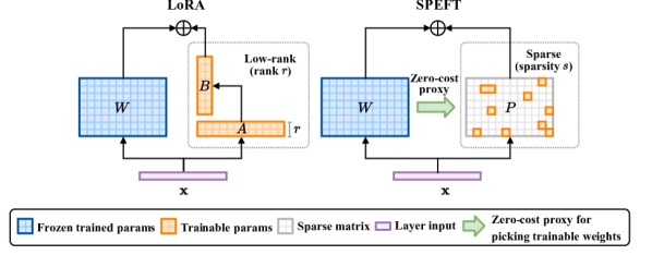
Figure 1: Comparison between LoRA [15] and SPEFT. LoRA freezes pretrained weights ${\bm{\theta}}_{0}$ and updates the low-rank terms $A$ and $B$, while SPEFT adopts zero-cost proxies to build a sparse adapter ${\bm{\theta}}_{\mathrm{sp}}$, to update the weight elements that contribute most to the downstream task.

Existing effort on PEFT methods mainly focuses on two categorizes, low-rank-based and sparsity-based adaptation approaches. LoRA [15], a popular low-rank adaptation method reparameterizes the model weight of each layer (${\bm{\theta}}\in\mathbb{R}^{d_{1}\times d_{2}}$) as ${\bm{\theta}}\triangleq{\bm{\theta}}_{0}+BA$, where ${\bm{\theta}}_{0}$ denotes the pretrained weight matrix which remains fixed during fine-tuning, $B\in\mathbb{R}^{d_{1}\times r}$ and $A\in\mathbb{R}^{r\times d_{2}}$ are trainable weights of a lower rank with $r\ll\min\{d_{1},d_{2}\}$. Recently, sparsity-based PEFT (SPEFT) has emerged as an alternative approach which constructs an alternate reparameterization, ${\bm{\theta}}\triangleq{\bm{\theta}}_{0}+{\bm{\theta}}_{\mathrm{sp}}$, where ${\bm{\theta}}_{\mathrm{sp}}$ is an extremely sparse matrix, and updates solely its non-zero entries. Figure˜1 illustrates the distinction between the two categories of PEFT methods. Previous sparse PEFT methods [12, 30, 2] have employed various first- and second-order metrics for determining these non-zero entries and adopted distinct approaches for handling the sparsity mask during training. The varying constructions and training-time treatments of the sparsity mask lead us to the following research questions on the basic design principles for SPEFT:

• Which salience metric or proxy is optimal for determining a sparsity mask?

• Is a static mask determined prior to the start of training sufficient, or is a dynamically updated pruning mask preferable?

In this paper, we systematically re-examine the design principles for SPEFT and conduct an evaluation across distinct salience metrics. Drawing inspiration from recent advancements in zero-cost Network Architecture Search (NAS) proxies, which explore diverse low-cost proxies for determining parameter importance that has incorporated both first-order (e.g.missing, weight magnitude, gradients, SNIP [21], etc.missing) and second-order estimators (e.g.missing, GRaSP [35], Fisher information [30], etc.missing), we discovered that these NAS proxies encompasses many salience metrics used in SPEFT for sparsity mask construction (DiffPruning [12], FishMASK [30], etc.missing). Consequently, inspired by recent zero-cost NAS metrics that have shown strong performance to construct sparsity masks, we are the first to comprehensively evaluate 8 different salience metrics in the context of SPEFT for LLMs. Furthermore, we investigate both dynamic and static masking approaches, where a dynamic mask matrix ${\bm{\tau}}$ changes during training, while a static mask maintains a static ${\bm{\tau}}$ binary matrix throughout the PEFT process. We make the following contributions:

• We systematically evaluate 8 different salience metrics for constructing sparsity masks in SPEFT and empirically show that gradient-based SPEFT offers strong performance, while second-order metrics, such as Fisher information, do not significantly enhance SPEFT performance.

• We found that dynamic masking strategies do not surpass the effectiveness of a simple static mask predefined before training in SPEFT. This approach affords greater acceleration opportunities, as fixed indices are predetermined and this avoids the mask re-computation cost.

• Our results indicate that a simple gradient-based, static SPEFT method delivers the best trade-off between effectiveness and efficiency. For instance, for RoBERTa-base on MRPC task, our method achieves 0.98% higher than the baseline given the same amount of trainable parameters. Gradient-based SPEFT outperforms LoRA by 22.6% on GSM8k [7] when trained on MetaMathQA [38]. Consequently, we advocate for this SPEFT variant to be considered a strong baseline for subsequent developments in this field.

2 Related Work

2.1 PEFT Methods

With the advent of large language models, fine-tuning these models on downstream tasks can be prohibitively expensive due to the sheer number of trainable parameters. A suite of parameter-efficient fine-tuning (PEFT) methods have been proposed to address this issue.

Low-rank adaptation [15] is a popular method in PEFT which reparameterizes the weight matrix of each layer (${\bm{\theta}}\in\mathbb{R}^{d_{1}\times d_{2}}$) as ${\bm{\theta}}={\bm{\theta}}_{0}+BA$. Here, ${\bm{\theta}}_{0}\in\mathbb{R}^{d_{1}\times d_{2}}$ is the pretrained weight matrix, and $B\in\mathbb{R}^{d_{1}\times r}$ and $A\in\mathbb{R}^{r\times d_{2}}$ are lower-rank matrices with $r\ll\min(d_{1},d_{2})$. By making only $A$ and $B$ trainable, this method significantly reduces the number of trainable parameters, thereby lowering computational resource requirements. LoRA has demonstrated effectiveness in reducing trainable parameters for fine-tuning large language models, while maintaining strong fine-tuned performance across various downstream tasks compared to full fine-tuning.

Sparsity-based adaptation Since the advent of low-rank adaptation, sparsity-based adaptation has emerged as an alternative approach to PEFT. It constructs sparse trainable matrix ${\bm{\theta}}_{\mathrm{sp}}$ reparameterization for each layer weight ${\bm{\theta}}={\bm{\theta}}_{0}+{\bm{\theta}}_{\mathrm{sp}}$, where $\lvert{\bm{\theta}}_{\mathrm{sp}}\rvert_{0}\leq s\ll d_{1}\times d_{2}$, and $s$ represents the number of non-zero entries. The gradient updates only happen to the non-zero entries of the sparse matrices during fine-tuning. Since the sparse matrix ${\bm{\theta}}_{\mathrm{sp}}$ is typically constructed to be extremely sparse, this approach can also achieve notable parameter efficiency, and the sparsity masking strategy plays a crucial role in determining impactful trainable parameters for fine-tuning.

This approach has been explored in various forms in the literature. Earlier works such as DiffPruning [12] learns a sparsity mask with straight-through gradient estimator [3, 16] to select important parameters for downstream tasks. FishMASK [30] applies a static sparsity mask from training outset, guided by Fisher information to measure sparsity. Beyond static masks, Fish-DIP [8] further allows the Fisher information-based mask to be updated dynamically during training. Inspired by the lottery ticket hypothesis [11], LF-SFT [2] finds that sparse masks obtained by selecting the parameters with the largest changes after fine-tuning on a task can be transferred to other tasks. However, this approach requires full fine-tuning on an initial task, which may not be feasible for resource-constrained settings. This paper explores the design principles for constructing the sparsity mask with low-cost salience metrics and the impact of dynamic versus static masks on the fine-tuning process.

Finally, sparsity-based adapters also allows highly granular control over trainable parameters, and can enable the use of existing knowledge transfer techniques, such as mixtures of sparse experts [36] and multi-task learning with sparse masks [29] in LLMs.

2.2 Salience Proxies for Sparsity Masking

The extensive research on low-cost salience metrics for fine-grained network pruning has provided a rich set of pruning-at-initialization metrics to determine the importance of neural network parameters. These metrics can be broadly classified into first- and second-order categories. First-order metrics include weight magnitude [13], connection sensitivity (SNIP) [20], foresight connection sensitivity (FORCE) [9], Taylor-FO [26], SynFlow [31], and finally, the gradient of the loss with respect to the weight. Second-order metrics comprise GRaSP [35] and Fisher information-based metrics [22]. Coincidentally, both FishMASK [30] and Fish-DIP [8] propose to use Fisher information to construct the sparsity mask: while FishMASK uses a static mask, Fish-DIP further allows the mask to be updated periodically during fine-tuning. These metrics are designed to identify important parameters or connections in a neural network. In this paper, we explore the impact of these salience metrics on fine-tuning by using them to construct sparse masks for PEFT.

3 Method

3.1 Problem Formulation

Given a pretrained model $f_{{\bm{\theta}}_{0}}$ with initial parameters ${\bm{\theta}}_{0}$, a dataset $\mathcal{D}_{\textrm{train}}$, and a downstream task loss function $\operatorname{\mathcal{L}}$, the goal of sparse parameter-efficient fine-tuning (SPEFT) is to find a set of sparse trainable parameters ${\bm{\theta}}_{\mathrm{sp}}$, that minimizes the loss function on the training dataset $\mathcal{D}_{\textrm{train}}$:

$${\bm{\theta}}_{\mathrm{sp}}^{\star}={\operatorname*{arg\,min}}_{{\bm{\theta}}_{\mathrm{sp}}}\mathbb{E}_{\lparen{\mathbf{x}},y\rparen\sim\mathcal{D}_{\textrm{train}}}\left[\operatorname{\mathcal{L}}\lparen f_{{\bm{\theta}}_{0}+{\bm{\theta}}_{\mathrm{sp}}}({\mathbf{x}});y\rparen\right].$$ (1)

To ensure the sparsity of ${\bm{\theta}}_{\mathrm{sp}}$, we constrain it with $\operatorname{\mathbf{1}}[{\bm{\theta}}_{\mathrm{sp}}\neq 0]={\bm{\tau}}$, where $\operatorname{\mathbf{1}}[\cdot]$ is the indicator function, ${\bm{\tau}}\in\{0,1\}^{d_{1}\times d_{2}}$ is the sparsity mask with $\lvert{\bm{\tau}}\rvert_{0}\leq{\rho}\ll d_{1}\times d_{2}$, where ${\rho}$ is the number of non-zero entries. This opens up the flexibility of ${\bm{\tau}}$ design, i.e.missing, selecting the non-zero locations in ${\bm{\theta}}_{\mathrm{sp}}$ to update during fine-tuning, which can be determined by various salience metrics as discussed below in Section˜3.2.

3.2 Salience Metrics

In this section, we describe the 8 salience metrics which can be used to determine the importance of weights ${\bm{\theta}}$. Assume that ${\mathbf{x}}$ is the sampled input, $\ell\triangleq\operatorname{\mathcal{L}}\lparen f_{\bm{\theta}}({\mathbf{x}});y\rparen$ is the loss function, $\odot$ denotes element-wise multiplication, and $\lvert\cdot\rvert$ denotes the element-wise absolute value. For simplicity, we also assume all data-aware metrics to be expectations over the training dataset $\lparen{\mathbf{x}},y\rparen\sim\mathcal{D}_{\textrm{train}}$, which can be approximated by sampling from it. We have the following 6 1^st-order salience metrics:

• Magnitude: $\lvert{\bm{\theta}}\rvert$, where simply the magnitude (i.e.missing, absolute value) of the weight is used.

• Gradient: $\frac{\partial{\ell}}{\partial{{\bm{\theta}}}}$, which is the gradient of the loss with respect to the weight ${\bm{\theta}}$.

• SNIP (single-shot network pruning): $\left\lvert\frac{\partial{\ell}}{\partial{{\bm{\theta}}}}\odot{\bm{\theta}}\right\rvert$, the connection sensitivity metric proposed in [20] to determine the importance of weights.

• FORCE (foresight connection sensitivity): $-\frac{\partial{\ell}}{\partial{{\bm{\theta}}}}\odot{\bm{\theta}}$, introduced in [9].

• Taylor-FO (Taylor first-order expansion): $\left\lparen\frac{\partial{\ell}}{\partial{{\bm{\theta}}}}\odot{\bm{\theta}}\right\rparen^{2}$, derived from the 1^st-order Taylor expansion of the loss [26].

• SynFlow (iterative synaptic flow pruning): $\frac{\partial{}}{\partial{{\bm{\theta}}}}\left[\mathbf{1}^{\top}\left\lparen\Pi_{l=1}^{L}\lvert{\bm{\theta}}^{(l)}\rvert\right\rparen\mathbf{1}\right]\odot{\bm{\theta}}$, where ${\bm{\theta}}^{(l)}$ denotes the weights of the $l$^th layer, and $L$ denotes the number of layers. A data-free metric proposed in [31] to model synaptic flow.

In addition, the 2^nd-order salience metrics are computed as follows, where $H\triangleq\frac{\partial^{2}\!\operatorname{\mathcal{L}}\lparen f_{\bm{\theta}}({\mathbf{x}});y\rparen}{\partial{\bm{\theta}}\partial{\bm{\theta}}^{\top}}$ denotes the Hessian matrix:

• GRaSP (gradient signal preservation): $-\left\lparen H\frac{\partial{\ell}}{\partial{{\bm{\theta}}}}\right\rparen\odot{\bm{\theta}}$, which is a 2^nd-order metric proposed in [35] that aims to preserve gradient signals rather than the loss value.

• Fisher information: $\left\lparen\frac{\partial{\ell}}{\partial{{\bm{\theta}}}}\right\rparen^{2}$, which uses the Fisher information to determine the importance of weights [30, 8].

3.3 Sparsity Masking

Global Sparsity Masking Given a salience metric $\operatorname{\mathcal{S}}({\bm{\theta}})$ of the weight ${\bm{\theta}}$ defined in Section˜3.2, we can construct the sparse binary mask ${\bm{\tau}}$ by selecting the top ${\rho}\in(0,1]$ fraction of the salience metric values, i.e.missing, ${\rho}$ denotes the density level, namely:

$${\bm{\tau}}=\operatorname{\mathbf{1}}\left[{\mathbf{s}}\geq\operatorname{\textrm{top}}_{\rho}\lparen{\mathbf{s}}\rparen\right],\text{where}\,{\mathbf{s}}=\operatorname{\mathcal{S}}({\bm{\theta}}).$$ (2)

Here $\operatorname{\mathbf{1}}$ is the indicator function, and $\operatorname{\textrm{top}}_{\rho}$ selects the top ${\rho}$ values.

Local Sparsity Masking Instead of ranking the salience metric values across all weight values, alternatively, we can construct layer-wise masks ${\bm{\tau}}^{(l)}$ for the individual weights ${\bm{\theta}}^{(l)}$ in each layer $l$, where each layer has a shared sparsity ${\rho}$, and the top ${\rho}$ values are selected from the salience metric values of the weights in that layer:

$${\bm{\tau}}^{(l)}=\operatorname{\mathbf{1}}\left[{\mathbf{s}}^{(l)}\geq\operatorname{\textrm{top}}_{\rho}\lparen{\mathbf{s}}^{(l)}\rparen\right],\text{where}\,{\mathbf{s}}^{(l)}=\operatorname{\mathcal{S}}({\bm{\theta}}^{(l)}).$$ (3)

Here, ${\bm{\theta}}$ is decomposed into layer-wise weights $\left[{\bm{\theta}}^{(1)},\ldots,{\bm{\theta}}^{(L)}\right]$ and ${\bm{\tau}}^{(l)}$ and ${\bm{\theta}}^{(l)}$ respectively denotes the mask and weights of the $l$^th layer.

3.4 Static vs.missing Dynamic Masks

Beyond generating a static mask using the above approach prior to fine-tuning, which remains fixed throughout the training process, we can also explore the use of dynamic masks, which are updated periodically during training. The dynamic mask can be refreshed at specific intervals by the following procedure: first, we apply the current trained weights to the model; we then re-rank the salience metric values with these weights, the top ${\rho}$ values are then selected to form a new mask using the updated salience metric values; subsequently, the fine-tuning process continues with the new mask. Notably, after updating the dynamic masks, we also need to reinitialize memory-based optimizers in order to avoid applying incorrect momentum values to the newly adapted sparse weights.

3.5 The SPEFT Algorithm

Algorithm 1 Sparse Parameter-Efficient Fine-Tuning (SPEFT)

1:Pretrained model $f_{{\bm{\theta}}_{0}}$, training dataset $\mathcal{D}_{\textrm{train}}$, batch size $B$, loss function $\operatorname{\mathcal{L}}$, salience metric $\operatorname{\mathcal{S}}$, sparsity level ${\rho}$, fine-tuning steps $T$, fine-tuning learning rate $\alpha$, mask update interval $I$

2:${\bm{\theta}}_{\mathrm{sp}}\leftarrow\mathbf{0};{\bm{\theta}}\leftarrow{\bm{\theta}}_{0}$ $\triangleright$ Initialize weights

3:for $t=1$ to $T$ do $\triangleright$ For each fine-tuning step…

4:  if $t=1\vee\lparen I\geq 0\wedge\lparen t\!\mod I=0\rparen\rparen$ then $\triangleright$ If salience masks should update… (Section˜3.4)

5:   $\lparen{\bm{\theta}},{\bm{\theta}}_{\mathrm{sp}}\rparen\leftarrow\lparen{\bm{\theta}}+{\bm{\theta}}_{\mathrm{sp}},\mathbf{0}\rparen$ $\triangleright$ Apply sparse weights to model

6:   ${\mathbf{s}}\leftarrow\operatorname{\mathcal{S}}({\bm{\theta}})$ $\triangleright$ Compute salience values for all weights (Section˜3.2)

7:   ${\bm{\tau}}\leftarrow\operatorname{\mathbf{1}}\left[{\mathbf{s}}\geq\operatorname{\textrm{top}}_{{\rho}}\lparen{\mathbf{s}}\rparen\right]$ $\triangleright$ Update mask by top-${\rho}$ values (Section˜3.3)

8:  end if

9:  $\lparen{\mathbf{x}}_{[1:B]},y_{[1:B]}\rparen\leftarrow\operatorname{minibatch}(\mathcal{D}_{\textrm{train}})$ $\triangleright$ Sample mini-batch

10:  $\ell\leftarrow\frac{1}{B}\sum_{b=1}^{B}\operatorname{\mathcal{L}}\lparen f_{{\bm{\theta}}+{\bm{\theta}}_{\mathrm{sp}}}({\mathbf{x}}_{b});y_{b}\rparen$ $\triangleright$ Forward pass

11:  ${\bm{\theta}}_{\mathrm{sp}}\leftarrow\mathrm{Opt}\left\lparen\alpha,{\bm{\theta}}_{\mathrm{sp}},{\bm{\tau}}\odot\frac{\partial{\ell}}{\partial{{\bm{\theta}}_{\mathrm{sp}}}}\right\rparen$ $\triangleright$ Parameter-efficient optimization of sparse weights

12:end for$\triangleright$ NOTE: only need to compute non-zero entries of ${\bm{\tau}}$ for the gradient

13:return ${\bm{\theta}}+{\bm{\theta}}_{\mathrm{sp}}$ $\triangleright$ Return fine-tuned model

Algorithm˜1 provides an overview of the proposed SPEFT algorithm to fine-tune models with sparse weight adaptations. The algorithm takes as input a pretrained model $f_{{\bm{\theta}}_{0}}$, an optimizer $\mathrm{Opt}$, a training dataset $\mathcal{D}_{\textrm{train}}$, a batch size $B$, a loss function $\operatorname{\mathcal{L}}$, a salience metric $\operatorname{\mathcal{S}}$, a sparsity level ${\rho}$, the number of fine-tuning steps $T$, the learning rate $\alpha$, and the mask update interval $I$. The algorithm begins by initializing the sparse weights ${\bm{\theta}}_{\mathrm{sp}}$ to zero (line 1), and then iterates for $T$ steps (line 2). In each iteration, the algorithm first checks if it is the initial iteration, which requires updating the mask, or if it is at the correct interval for iterative dynamic mask updates (line 3). If either of these conditions is true, the algorithm applies the current sparse weights to the model (line 4), evaluates the new salience values ${\mathbf{s}}$ (line 5), and updates the salience mask ${\bm{\tau}}$ for the updated weights, on the sparsity level ${\rho}$ (line 6). After updating the mask, the training step follows by sampling a mini-batch $\{{\mathbf{x}},y\}$ from the training dataset (line 8), and learns the sparse weights ${\bm{\theta}}_{\mathrm{sp}}$ (line 9) using the optimizer $\mathrm{Opt}$ (e.g.missing, stochastic gradient descent, Adam, etc.missing). Here, ${\bm{\tau}}\odot\alpha\frac{\partial{\ell}}{\partial{{\bm{\theta}}_{\mathrm{sp}}}}$ where $\odot$ denotes element-wise multiplication. In terms of actual implementation, only the non-zero entries in $\frac{\partial{\ell}}{\partial{{\bm{\theta}}_{\mathrm{sp}}}}$ dictated by the mask ${\bm{\tau}}$ are computed and updated. Finally, the algorithm returns the fine-tuned model ${\bm{\theta}}_{0}+{\bm{\theta}}_{\mathrm{sp}}$.

4 Experimental Results

Models

We evaluated our approaches and baselines over a set of models, including fine-tuned OPT variants (-125m, -350m, and -1.3b) [39], BERT-base-uncased [10] and RoBERTa-base [23], for the GLUE [34] benchmark, and fine-tuned Gemma2-2b [33] and Qwen2-7b [37], to evaluate on the Massive Multitask Language Understanding (MMLU) benchmark [14] and GSM8K [7], a dataset of grade school math problems. In addition to sparse PEFT methods presented in this paper, we further include LoRA [15] and PiSSA [25] as low-rank adapter baselines for comparison.

Benchmarks

To show the generality of our approach, we chose GLUE, MMLU and GSM8K as benchmarks for evaluation. For the GLUE [34] benchmark, six representative tasks with large sizes are selected: single-sentence task SST-2, inference tasks QNLI, MNLI, similarity and paraphrase tasks MRPC, STS-B and QQP. For the MMLU [14] benchmark, it contains questions covering 57 subjects across STEM, the humanities, the social sciences, and others. It is designed to test the model’s ability to handle various types of language data and complex problems. We fine-tuned Gemma-2-2b, Qwen2-7b on either the Alpaca [32] or OASST2 [17] conversational datasets, and then evaluated them on all tasks in MMLU. We fine-tuned Gemma2-2b on the MetaMathQA [38] dataset and evaluated on GSM8K (8-shots) to assess the models’ multi-step mathematical reasoning ability. In the results, we reported the match accuracy for MNLI, Pearson correlation for STS-B, flexible extract and strict match scores for GSM8K, and accuracy values for other tasks.

Baselines

We chose LoRA [15] and PiSSA [25] as the competing low-rank baselines across models and benchmarks. By default in all comparisons, SPEFT methods use global sparsity ranking with static masks. For statistical significance, we repeated each experiment 3 times for OPT-{125m,350m}, BERT-base-uncased, and RoBERTa-base, and reported average metrics and their standard deviations.

Ablation Analyses

We also used the most reliable salience metric, i.e.missing, gradient-based, in further experiments to explore questions related to dynamic vs.missing static masks, and global vs.missing local sparsity in Section˜4.3.

Hyperparameters

Our SPEFT methods introduce a hyperparameter ${\rho}$, the percentage of trainable parameters. To ensure a fair comparison, we fixed ${\rho}$ of our SPEFT methods to use the same amounts of trainable parameters as LoRA and PiSSA on every model, and kept the remaining hyperparameters always the same. For example, for the RoBERTa-base model, we performed a grid sweep over learning rates from $5\times 10^{-4}$ to $5\times 10^{-5}$ to search for the best. Details about the hyperparameter settings can be found in Appendix˜A.

4.1 Main Results

Our experiments results on OPT-350m and BERT-base-uncased can be seen in Table˜1. For additional results on RoBERTa-base, OPT-125m and OPT-1.3b, please refer to Tables˜8, 9 and 10 in Appendix˜B. Across all models, we observed that among all the approaches, gradient-based SPEFT has the best average accuracy, higher than LoRA and PiSSA. For instance, in OPT-125m and OPT-350m, gradient-based SPEFT achieves $86.92\%$ and $88.45\%$, that are higher than the best competing SPEFT methods by $0.73\%$ and $0.85\%$ respectively. Particularly on OPT-350m, gradient-based SPEFT has the best performance on MNLI, MRPC, SST-2, and STS-B, On QNLI and QQP, LoRA has the best performance while gradient-based SPEFT has a good performance close to it. This shows that although LoRA shows excellent performance on certain tasks, SPEFT methods, particularly with the gradient salience metric, could further push the limit, achieving better results in accuracy. On BERT-base-uncased, we found that while SPEFT with Fisher-Info salience metric outperforms gradient-based SPEFT on QNLI, QQP and SST-2, it has a large gap in performance in the remaining tasks, making gradient-based SPEFT a more reliable and desirable choice. Similar results are also observed for other OPT variants in Tables˜9 and 10 and RoBERTa-base in Table˜8 of Appendix˜B.

Table 1: Comparing the salience metrics on OPT-350m (with 0.35% trainable parameters) and BERT-base-uncased (with 0.27% trainable parameters) for various GLUE tasks. For reference, we provide the LoRA and PiSSA baselines with the same number of trainable parameters for each model. The “#” column denotes the number of best performing tasks for each method. The best result of each column is highlighted in bold. “Avg.” reports the average score across all tasks, and their average standard deviations.

Method MNLI MRPC QNLI QQP SST-2 STS-B Avg. # OPT-350m (Trainable = 0.35%) LoRA 83.56$\pm$.07 84.56$\pm$.49 89.69$\pm$.11 89.66$\pm$.04 93.87$\pm$.06 88.57$\pm$.99 88.32$\pm$.29 2 PiSSA 83.45$\pm$.06 83.09$\pm$.52 89.38$\pm$.06 89.66$\pm$.02 93.58$\pm$.09 88.39$\pm$.52 87.93$\pm$.21 1 Magnitude 79.34$\pm$.41 71.57$\pm$.13 86.45$\pm$.06 87.68$\pm$.01 91.98$\pm$.12 45.04$\pm$3.39 77.01$\pm$.51 0 Gradient 83.86$\pm$.06 84.80$\pm$.55 89.68$\pm$.01 89.51$\pm$.01 93.93$\pm$.12 88.95$\pm$.25 88.45$\pm$.02 3 SynFlow 77.45$\pm$.05 77.94$\pm$.49 83.19$\pm$.03 88.03$\pm$.02 92.32$\pm$.18 79.18$\pm$.63 83.02$\pm$.22 0 SNIP 83.40$\pm$.05 83.09$\pm$.37 89.68$\pm$.22 89.37$\pm$.02 93.75$\pm$.06 86.32$\pm$.04 87.60$\pm$.10 0 FORCE 83.25$\pm$.08 82.60$\pm$.62 89.75$\pm$.30 89.50$\pm$.03 94.04$\pm$.69 85.53$\pm$.18 87.44$\pm$.26 0 Taylor-FO 83.31$\pm$.08 83.09$\pm$.37 89.68$\pm$.22 89.37$\pm$.02 93.75$\pm$.06 86.32$\pm$.04 87.59$\pm$.12 0 GRaSP 74.78$\pm$.27 83.58$\pm$.49 84.46$\pm$.39 89.38$\pm$.03 94.04$\pm$.01 86.97$\pm$.01 85.54$\pm$.20 1 Fisher-Info 35.45$\pm$1.35 84.31$\pm$.61 88.12$\pm$.34 86.34$\pm$.41 87.16$\pm$.35 88.61$\pm$.02 78.33$\pm$.51 0 BERT-base-uncased (Trainable = 0.27%) LoRA 81.45$\pm$.41 88.48$\pm$1.03 89.57$\pm$.35 87.77$\pm$.54 91.82$\pm$.14 84.07$\pm$1.11 87.19$\pm$.30 1 PiSSA 81.08$\pm$.27 87.75$\pm$.43 90.19$\pm$.30 88.14$\pm$.33 91.51$\pm$.08 85.12$\pm$.26 87.30$\pm$.18 1 Magnitude 77.09$\pm$.24 68.88$\pm$.25 86.60$\pm$.07 85.56$\pm$.50 90.14$\pm$.02 37.59$\pm$1.93 74.31$\pm$.33 0 Gradient 80.99$\pm$.12 89.46$\pm$.48 89.90$\pm$.26 87.48$\pm$.13 91.63$\pm$.01 85.08$\pm$.06 87.42$\pm$.15 2 SynFlow 70.85$\pm$.21 71.33$\pm$.25 83.49$\pm$.04 83.69$\pm$.16 90.08$\pm$.29 74.55$\pm$.36 79.00$\pm$.12 0 SNIP 80.74$\pm$.20 79.90$\pm$1.47 89.39$\pm$.08 87.27$\pm$.25 91.57$\pm$.06 80.92$\pm$.41 84.96$\pm$.18 0 FORCE 80.25$\pm$.09 78.31$\pm$.86 88.98$\pm$.15 87.04$\pm$.38 91.57$\pm$.17 79.21$\pm$.24 84.23$\pm$.15 0 Taylor-FO 80.74$\pm$.20 79.90$\pm$1.47 89.39$\pm$.08 87.27$\pm$.25 91.57$\pm$.06 80.87$\pm$.46 84.96$\pm$.18 0 GRaSP 79.37$\pm$.27 77.95$\pm$1.72 87.50$\pm$1.12 87.03$\pm$.41 91.35$\pm$.52 79.67$\pm$1.43 83.81$\pm$.59 0 Fisher-Info 79.83$\pm$.16 87.75$\pm$.74 90.46$\pm$.22 88.78$\pm$.25 91.86$\pm$.34 82.79$\pm$.63 86.91$\pm$.18 3

Notably, for both causal and masked language models, sparsity-based PEFT can outperform low-rank adapters, and the gradient-based SPEFT shows the strongest performance compared to other methods, closely followed by LoRA and PiSSA, which is consistent across all models. In addition, the gradient-based SPEFT outperformed LoRA and PiSSA in several tasks, highlighting its effectiveness across different model sizes. The comprehensive results table for these models and tasks underlines the consistent performance edge of gradient-based SPEFT, making it a reliable choice for a wide range of NLP tasks.

4.2 Larger Scale Models

For larger models, we evaluated all methods on Gemma2-2b and Qwen2-7b, and show the results in Table˜2. The results indicate that larger models can also benefit from SPEFT with the gradient-based saliency method, which outperforms other sparse training methods and LoRA.

Table 2: Comparing the salience metrics on Gemma2-2B and Qwen2-7B respectively with 0.97% and 0.53% trainable parameters. We fine-tuned models on either Alpaca or OASST2 and evaluated on 5-shot MMLU. For reference, we provide the LoRA baselines with the same number of trainable parameters for each combination.

Model Gemma2-2B Qwen2-7B Avg. Dataset Alpaca OASST2 Alpaca OASST2 LoRA 53.07 52.59 69.77 70.42 61.46 Gradient 53.11 53.11 70.96 70.55 61.93 SynFlow 52.84 53.07 69.80 70.66 61.59 Magnitude 52.97 53.03 70.12 70.76 61.72 SNIP 52.81 52.89 68.75 70.52 61.24 FORCE 52.79 52.88 69.01 70.53 61.30 Taylor-FO 52.81 52.96 68.75 69.10 60.91 GRaSP 52.38 52.60 66.69 69.91 60.40 Fisher-Info 52.70 52.65 66.45 69.10 60.23

To evaluate on the text generation task, We fine-tuned Gemma2-2B with our methods We also provide the results of the pretrained model (without fine-tuning) and LoRA as baselines. The results are shown in Table˜3. It can be seen that the sparse adapters outperformed the LoRA baseline, with the gradient-based SPEFT method leading the pack with the best performance. Notably, the lead by sparse adapters widens as the task complexity increases, which demands token sequence generation with multi-step reasoning.

Table 3: Comparing the salience metrics on Gemma2-2B with 0.97% trainable parameters. We fine-tuned the model on MetaMathQA and evaluated on 8-shot GSM8K. For reference, we provide pretrained model (without fine-tuning) and the LoRA baseline with the same number of trainable parameters.

Method Flexible Extract Strict Match Avg. Pretrained 24.56 17.66 21.11 LoRA 39.20 28.81 34.00 Gradient 50.27 37.15 43.71 SynFlow 37.76 27.75 32.75 Magnitude 37.45 27.07 32.26 SNIP 39.80 29.64 34.72 FORCE 39.88 29.95 34.91 Taylor-FO 40.33 30.25 35.29 GRaSP 50.15 37.03 43.59 Fisher-Info 41.47 30.25 35.86

4.3 Exploration of masking strategies

Table 4: Results of OPT-125m, OPT-350m and BERT-base-uncased with fixed or dynamic gradient masks and global or local sparsity on various GLUE tasks. The dynamic strategy will update the gradient mask every 1000 train steps. “S / D”: static / dynamic masks, “G / L”: global / local sparsity. Runs were repeated 3 times and all results have a standard deviation of $<0.5\%$.

MNLI MRPC QNLI QQP SST-2 STS-B Avg. OPT-125m (Trainable = 0.35%) SG 81.41 83.82 88.58 88.71 91.44 87.55 86.92 SL 81.41 81.86 88.94 88.76 91.40 87.38 86.63 DG 77.71 82.84 83.80 87.36 89.33 88.28 84.89 DL 69.26 73.53 80.56 84.82 86.35 87.15 80.28 OPT-350m (Trainable = 0.35%) SG 83.86 84.80 89.68 89.51 93.93 88.95 88.46 SL 84.31 83.33 90.63 90.97 94.50 88.52 88.71 DG 78.03 85.29 89.22 84.24 91.51 88.54 86.14 DL 78.86 71.57 80.84 84.52 87.27 87.52 81.76 BERT-base-uncased (Trainable = 0.27%) SG 80.99 89.46 89.90 87.48 91.63 85.08 87.42 SL 74.58 85.54 89.62 83.41 91.06 85.79 85.00 DG 83.17 89.46 90.32 90.27 92.20 84.20 88.27 DL 72.80 86.52 83.49 82.51 90.25 85.95 83.59

Based on the comparisons with SPEFT in Section˜4.1, which showed that gradient-based SPEFT is the best-performing method, we would use it for ablation studies of dynamic vs.missing static masks, and global vs.missing local sparsity. In this section, we delve into the comparisons between between global and local sparsity (Section˜3.3) and also static and dynamic masking strategies (Section˜3.4) using gradient-based SPEFT, the best-performing salience metric, across OPT-125m, OPT-350m, and BERT-base-uncased. Here, we periodically update the masks every $I=1000$ steps with 1024 training examples to estimate the salience metrics. The results are shown in Table˜4.

Dynamic vs.missing static masking

The findings reveal that dynamic masking offers only a slight performance advantage in smaller models like BERT-base-uncased but does not significantly outperform static masking in larger models. For instance, on OPT-350m, we actually see static masking provides us a better averaged accuracy ($88.46$ and $88.71$) compared to dynamic masking ($86.14$ and $81.76$). Given that dynamic masking requires more computational resources, because of the periodic update on sparsity masks, the marginal performance gain does not justify the extra cost, especially for larger models. Therefore, static masking emerges as a more practical and resource-efficient strategy, providing substantial performance benefits without the additional computational overhead.

Global vs.missing local sparsity

With global sparsity, SPEFT calculates the metrics across all transformer layers, ranks them collectively, and makes only the highest-ranked ones trainable. In the local approach, metrics are sorted and ranked within each individual layer. Our results showed no significant difference in performance between the two strategies. For instance, the results in BERT-base-uncased suggests that global is superior, by showing a better averaged accuracy across the six GLUE tasks, but the numbers in OPT-350m suggest the reverse under the static masking strategy.

4.4 Minimal Overhead for SPEFT

Computational overhead

For all first-order salience metrics, we use a few gradient evaluations to compute the salience scores. Specifically, only 64 steps with a batch size of 16 per estimation are needed (1024 examples), which is negligible compared to the overall training cost. For example, this represents only 0.26% and 0.97% of the training time for one epoch on MNLI and QNLI, respectively. For static masks, this computation is performed once before training; for dynamic masking, it is repeated once per $I=1000$ steps. Second-order metrics such as GRaSP and Fisher-Info require $2\times$ the number of gradient evaluations of first-order metrics to compute the second-order gradients. The magnitude metric requires no additional computation. Finally, we observed no statistically significant difference in training time between the sparse methods and the LoRA baseline.

Memory overhead

As we aligned the number of trainable parameters across LoRA and the SPEFT methods, the peak memory usage for both methods are mostly identical, except that the SPEFT methods require a small amount of additional memory overhead to store the indices in CSR format. In all experiments, the overhead is less than 0.5% of the peak memory usage.

5 Discussion

The Trend of Supporting Sparse Computation as Hardware Intrinsics

Numerous hardware vendors have introduced specialized hardware features with instruction set extensions tailored for sparse matrix multiplication. Especially in recently announced hardware devices. Mainstream devices like NVIDIA’s A100 [6], H100 [5], and H200, as well as offerings from other major vendors or emerging competitors such as AMD’s MI300 [1] and Cerebras’ WSE2 [27], are embracing this trend. As hardware support for sparse computation advances, the utility of sparsity-based PEFT, or generally sparse training, is poised to improve substantially. This development will enable both current and future strategies to attain performance levels closer to their full potential, as these calculations won’t require emulation via dense computations, allowing for closer realization of theoretical speedups and savings on FLOPs.

The Role of Salience Measurements

A fundamental element of this study involves reevaluating certain design choices in SPEFT, leading to the discovery that straightforward designs, such as first-order salience proxies, emerge as the most effective methods. Intriguingly, selecting the most salient weights in a neural network has being a long-standing challenge, one that dates back to early weight pruning research by LeCun et al.missing in 1989 [19]. It’s notable that the optimal saliency metric seems to differ – or arguably should differ – among different task setups, such as post-training weight pruning [19], pruning at initialization [21, 9], and zero-cost NAS proxies [28]. The suggested practice then should be to systematically review a range of known and established proxies to set a solid baseline before designing a complex salience metric.

6 Conclusion

We explored the efficacy of various sparse parameter-efficient fine-tuning (SPEFT) methods in enhancing the performance of LLMs. Our experiments compared LoRA and PiSSA against SPEFT methods with a range salience metrics, and demonstrated that gradient-based SPEFT consistently achieved superior accuracy across different tasks and model architectures. This demonstrates that, although LoRA and PiSSA is effective in certain contexts, SPEFT methods that leverage gradient information can further optimize performance. We also investigated the impact of static versus dynamic sparsity masks, concluding that while dynamic masks do not significantly outperform static masks, and they introduce additional training overhead. Our findings suggest that static masks, combined with the gradient-based salience metric, provide a practical balance between computational efficiency and model accuracy. Overall, our research contributes to the ongoing efforts in making model fine-tuning more efficient and accessible, particularly in resource-constrained settings.

7 Limitations

During the experiments, we found that in a few training runs, SPEFT seems less sensitive to hyperparameter changes than LoRA, i.e.missing, on a range of hyperparameter sets, SPEFT always improves model performance, but LoRA fails. Due to limited resources and time, we did not run additional experiments to explore this interesting observation. We leave this exploration for future work. Moreover, similar investigations on parameter efficient fine-tuning could be conducted with non-language-based models or other multimodal models, such as vision large language models (VLLMs), however, these explorations are beyond the current scope of this paper and thus is left as future work.

8 Computational Resources

We performed all experiments on a cluster of NVIDIA A100 40GB GPUs. The experiments took around 486 GPU-hours for a single model on all GLUE subsets and all salient metrics. Besides, it took around 40 GPU-hours for a single model on Alpaca or OASST2 training on all low-rank and sparse PEFT methods. It also took around 80 GPU-hours to train with all methods on MetaMath for GSM8k evaluation. We also spent around 500 GPU-hours aligning the baseline results with the literature and determining fine-tuning hyperparameters.

Appendix A Hyperparameters

The hyperparameters we used for all models are shown in Tables˜7, 6 and 5. Notably, for all models, the density ${\rho}$ was set to make sure the number of trainable parameters across all methods was the same as the LoRA baseline.

Table 5: The hyperparameters we used for Gemma2-2B on MetaMathQA.

Model Method Hyperparameters MetaMathQA Optimizer AdamW Shared Warmup Ratio 0.03 LR Schedule Linear Gemma2-2B (LoRA) Batch Size 16 # Epochs 1 Learning Rate 2E-5 LoRA $r$ 64 LoRA $\alpha$ 16 Max Seq. Len. 1024 Gemma2-2B (Sparse) Batch Size 16 # Epochs 1 Learning Rate 2E-5 Sparse Top $k$ 0.18% Max Seq. Len. 1024

Table 6: The hyperparameters we used for Gemma2-2B and Qwen2-7B on Alpaca and OASST2. The percentage of trainable parameters (${\rho}$) for the sparse models are chosen to be the same as the LoRA models.

Model (Method) Hyperparameters Alpaca OASST2 Shared Optimizer AdamW Warmup Ratio 0.03 LR Schedule Constant Batch Size 16 Max Seq. Len. 1024 Gemma2-2B (LoRA) # Steps 2000 Learning Rate 5E-5 LoRA $r$ 64 LoRA $\alpha$ 16 Gemma2-2B (Sparse) # Steps 2000 Learning Rate 1E-5 5E-6 Sparse ${\rho}$ 0.97% Qwen2-7B (LoRA) # Epochs/Steps 3 Epochs 2000 Steps Learning Rate 5E-5 LoRA $r$ 64 LoRA $\alpha$ 16 Qwen2-7B (Sparse) # Epochs/Steps 3 Epochs 2000 Steps Learning Rate 5E-5 5E-6 Sparse ${\rho}$ 0.53%

Table 7: The hyperparameters we used for all models evaluated on the GLUE benchmark. The percentage of trainable parameters (${\rho}$) for the sparse models are chosen to be the same as the LoRA models.

Method Dataset MRPC, STS-B QNLI, SST-2, MNLI, QQP Shared Optimizer AdamW AdamW Warmup Ratio 0 0 LR Schedule Linear Linear Batch Size 16 64 # Epochs 30 30 Learning Rate 4E-4 5E-5 Max Seq. Len. 512 196 LoRA LoRA $r$ 8 8 LoRA $\alpha$ 16 8 OPT-125m Sparse ${\rho}$ 0.35% 0.35% OPT-350m Sparse ${\rho}$ 0.35% 0.35% BERT-base Sparse ${\rho}$ 0.27% 0.27% RoBERTa-base Sparse ${\rho}$ 0.24% 0.24% Model (Method) Hyperparameters All datasets Shared Optimizer AdamW Warmup Ratio 0 LR Schedule Linear Learning Rate 5E-5 # Epochs 30 Batch Size 16 OPT-1.3b (LoRA) LoRA $r$ 8 LoRA $\alpha$ 8 OPT-1.3b (Sparse) Sparse ${\rho}$ 0.18%

Appendix B Additional Experimental Results

Tables˜8, 9 and 10 provide additional respective results on GLUE tasks for the OPT-125m and OPT-1.3b variants, and BERT-base-uncased.

Table 8: Comparing the salience metrics on RoBERTa-base for various GLUE tasks with 0.24% trainable parameters, following the same format as Table˜1.

Method MNLI MRPC QNLI QQP SST-2 STS-B Avg. # LoRA 86.52$\pm$.06 89.46$\pm$.73 92.11$\pm$.29 88.70$\pm$.15 93.81$\pm$.23 90.30$\pm$.01 90.15$\pm$.25 0 PiSSA 86.71$\pm$.02 89.47$\pm$.42 92.20$\pm$.09 88.46$\pm$.10 93.75$\pm$.14 90.78$\pm$.02 90.23$\pm$.13 3 Magnitude 82.58$\pm$.46 31.62$\pm$2.05 88.03$\pm$.35 86.37$\pm$.36 90.60$\pm$.23 15.16$\pm$2.64 65.73$\pm$1.01 0 Gradient 86.00$\pm$.05 90.44$\pm$.11 91.89$\pm$.13 88.78$\pm$.05 94.16$\pm$.06 90.29$\pm$.02 90.26$\pm$.04 2 SynFlow 75.53$\pm$.02 70.34$\pm$.12 84.37$\pm$.01 85.19$\pm$.02 91.80$\pm$.29 76.92$\pm$.44 80.69$\pm$.17 0 SNIP 85.97$\pm$.01 87.01$\pm$.25 91.34$\pm$.01 88.31$\pm$.06 93.92$\pm$.29 87.52$\pm$.16 89.01$\pm$.08 0 FORCE 85.64$\pm$.05 85.29$\pm$.37 91.31$\pm$.04 88.39$\pm$.04 93.75$\pm$.06 86.52$\pm$.15 88.48$\pm$.07 0 Taylor-FO 85.97$\pm$.01 87.01$\pm$.25 91.34$\pm$.01 88.31$\pm$.06 93.92$\pm$.29 87.52$\pm$.16 89.01$\pm$.08 0 GRaSP 79.07$\pm$.02 84.80$\pm$.25 87.88$\pm$.02 88.45$\pm$.12 93.52$\pm$.06 86.81$\pm$.24 86.76$\pm$.04 0 Fisher-Info 85.52$\pm$.15 86.76$\pm$.35 91.82$\pm$.06 89.16$\pm$.03 93.92$\pm$.28 87.51$\pm$.05 89.12$\pm$.15 1

Table 9: Comparing the salience metrics on OPT-125m with 0.35% trainable parameters on various GLUE tasks, following the same format as Table˜1.

Method MNLI MRPC QNLI QQP SST-2 STS-B Avg. # LoRA 81.94$\pm$.22 82.84$\pm$.23 88.23$\pm$.30 88.45$\pm$.20 91.97$\pm$.18 87.25$\pm$.47 86.78$\pm$.21 2 PiSSA 81.56$\pm$.11 83.33$\pm$.30 87.99$\pm$.32 88.17$\pm$.15 91.97$\pm$.11 86.87$\pm$.39 86.65$\pm$.15 1 Magnitude 78.03$\pm$3.14 76.35$\pm$4.05 85.46$\pm$1.62 86.56$\pm$1.15 90.40$\pm$.85 50.32$\pm$2.42 77.85$\pm$3.27 0 Gradient 81.41$\pm$.01 83.82$\pm$.37 88.58$\pm$.37 88.71$\pm$.09 91.46$\pm$.05 87.55$\pm$.34 86.92$\pm$.05 3 SynFlow 81.05$\pm$.05 81.01$\pm$.37 87.92$\pm$.07 88.35$\pm$.04 91.21$\pm$.14 85.47$\pm$.75 85.83$\pm$.16 0 SNIP 81.21$\pm$.01 81.62$\pm$.74 88.31$\pm$.12 88.58$\pm$.04 91.32$\pm$.53 86.11$\pm$.40 86.19$\pm$.06 0 FORCE 81.31$\pm$.09 79.91$\pm$.74 88.31$\pm$.08 88.46$\pm$.04 91.44$\pm$.23 85.62$\pm$.48 85.84$\pm$.02 0 Taylor-FO 81.21$\pm$.01 81.62$\pm$.74 88.31$\pm$.12 88.58$\pm$.04 91.32$\pm$.53 86.11$\pm$.40 86.19$\pm$.06 0 GRaSP 81.36$\pm$.14 81.25$\pm$.61 88.11$\pm$.03 88.52$\pm$.12 91.40$\pm$.28 85.69$\pm$.35 86.05$\pm$.20 0 Fisher-Info 74.43$\pm$.15 80.39$\pm$.61 80.63$\pm$.64 86.81$\pm$.03 87.50$\pm$.91 87.59$\pm$.38 72.31$\pm$.45 1

Table 10: Comparing the salience metrics on OPT-1.3b with 0.18% trainable parameters on a subset of the GLUE benchmark, following the same format as Table˜9.

Method MRPC QNLI SST-2 STS-B QQP Avg. # LoRA 83.33 92.48 95.99 89.03 89.97 90.16 1 Magnitude 77.45 90.43 95.18 80.33 90.41 86.76 1 Gradient 87.25 92.11 95.53 90.30 89.02 90.84 2 SynFlow 78.68 90.85 96.10 81.66 88.56 87.17 1 SNIP 83.82 92.48 75.23 89.44 85.93 85.38 1 FORCE 83.58 92.39 89.56 88.83 88.31 88.53 0 Taylor-FO 83.82 92.48 75.23 89.44 85.93 85.38 1 GRaSP 84.80 92.46 87.96 89.54 88.09 88.57 0 Fisher-Info 81.37 90.74 83.26 84.86 85.27 85.10 0

References

- [1] AMD Instinct MI300 Series Accelerators. https://www.amd.com/en/products/accelerators/instinct/mi300.html. Accessed: 2024-03-03.
- Ansell et al. [2021] Alan Ansell, Edoardo Maria Ponti, Anna Korhonen, and Ivan Vulić. 2021. Composable sparse fine-tuning for cross-lingual transfer. arXiv preprint arXiv:2110.07560.
- Bengio et al. [2013] Yoshua Bengio, Nicholas Léonard, and Aaron Courville. 2013. Estimating or propagating gradients through stochastic neurons for conditional computation. arXiv preprint arXiv:1308.3432.
- Brown et al. [2020] Tom Brown, Benjamin Mann, Nick Ryder, Melanie Subbiah, Jared D Kaplan, Prafulla Dhariwal, Arvind Neelakantan, Pranav Shyam, Girish Sastry, Amanda Askell, et al. 2020. Language models are few-shot learners. Advances in neural information processing systems, 33:1877–1901.
- Choquette [2023] Jack Choquette. 2023. NVIDIA Hopper H100 GPU: Scaling Performance. IEEE Micro, (3):9–17.
- Choquette et al. [2021] Jack Choquette, Wishwesh Gandhi, Olivier Giroux, Nick Stam, and Ronny Krashinsky. 2021. NVIDIA A100 tensor core GPU: Performance and innovation. IEEE Micro, (2):29–35.
- Cobbe et al. [2021] Karl Cobbe, Vineet Kosaraju, Mohammad Bavarian, Mark Chen, Heewoo Jun, Lukasz Kaiser, Matthias Plappert, Jerry Tworek, Jacob Hilton, Reiichiro Nakano, Christopher Hesse, and John Schulman. 2021. Training verifiers to solve math word problems. Preprint, arXiv:2110.14168.
- Das et al. [2023] Sarkar Snigdha Sarathi Das, Ranran Haoran Zhang, Peng Shi, Wenpeng Yin, and Rui Zhang. 2023. Unified low-resource sequence labeling by sample-aware dynamic sparse finetuning. arXiv preprint arXiv:2311.03748.
- de Jorge et al. [2021] Pau de Jorge, Amartya Sanyal, Harkirat Behl, Philip Torr, Grégory Rogez, and Puneet K. Dokania. 2021. Progressive skeletonization: Trimming more fat from a network at initialization. In International Conference on Learning Representations.
- Devlin et al. [2019] Jacob Devlin, Ming-Wei Chang, Kenton Lee, and Kristina Toutanova. 2019. Bert: Pre-training of deep bidirectional transformers for language understanding. Preprint, arXiv:1810.04805.
- Frankle and Carbin [2019] Jonathan Frankle and Michael Carbin. 2019. The lottery ticket hypothesis: Finding sparse, trainable neural networks.
- Guo et al. [2020] Demi Guo, Alexander M Rush, and Yoon Kim. 2020. Parameter-efficient transfer learning with diff pruning. arXiv preprint arXiv:2012.07463.
- Han et al. [2015] Song Han, Huizi Mao, and William J Dally. 2015. Deep compression: Compressing deep neural networks with pruning, trained quantization and huffman coding. arXiv preprint arXiv:1510.00149.
- Hendrycks et al. [2021] Dan Hendrycks, Collin Burns, Steven Basart, Andy Zou, Mantas Mazeika, Dawn Song, and Jacob Steinhardt. 2021. Measuring massive multitask language understanding. Preprint, arXiv:2009.03300.
- Hu et al. [2021] Edward J Hu, Yelong Shen, Phillip Wallis, Zeyuan Allen-Zhu, Yuanzhi Li, Shean Wang, Lu Wang, and Weizhu Chen. 2021. Lora: Low-rank adaptation of large language models. arXiv preprint arXiv:2106.09685.
- Hubara et al. [2016] Itay Hubara, Matthieu Courbariaux, Daniel Soudry, Ran El-Yaniv, and Yoshua Bengio. 2016. Binarized neural networks. Advances in neural information processing systems, 29.
- Köpf et al. [2023] Andreas Köpf, Yannic Kilcher, Dimitri von Rütte, Sotiris Anagnostidis, Zhi-Rui Tam, Keith Stevens, Abdullah Barhoum, Nguyen Minh Duc, Oliver Stanley, Richárd Nagyfi, Shahul ES, Sameer Suri, David Glushkov, Arnav Dantuluri, Andrew Maguire, Christoph Schuhmann, Huu Nguyen, and Alexander Mattick. 2023. Openassistant conversations – democratizing large language model alignment. Preprint, arXiv:2304.07327.
- Lan et al. [2019] Zhenzhong Lan, Mingda Chen, Sebastian Goodman, Kevin Gimpel, Piyush Sharma, and Radu Soricut. 2019. Albert: A lite bert for self-supervised learning of language representations. arXiv preprint arXiv:1909.11942.
- LeCun et al. [1989] Yann LeCun, John Denker, and Sara Solla. 1989. Optimal brain damage. Advances in neural information processing systems, 2.
- Lee et al. [2019a] Namhoon Lee, Thalaiyasingam Ajanthan, and Philip Torr. 2019a. SNIP: Single-shot network pruning based on connection sensitivity. In International Conference on Learning Representations.
- Lee et al. [2019b] Namhoon Lee, Thalaiyasingam Ajanthan, and Philip H. S. Torr. 2019b. Snip: Single-shot network pruning based on connection sensitivity. Preprint, arXiv:1810.02340.
- Liu et al. [2021] Liyang Liu, Shilong Zhang, Zhanghui Kuang, Aojun Zhou, Jing-Hao Xue, Xinjiang Wang, Yimin Chen, Wenming Yang, Qingmin Liao, and Wayne Zhang. 2021. Group fisher pruning for practical network compression. In International Conference on Machine Learning, pages 7021–7032. PMLR.
- Liu et al. [2019] Yinhan Liu, Myle Ott, Naman Goyal, Jingfei Du, Mandar Joshi, Danqi Chen, Omer Levy, Mike Lewis, Luke Zettlemoyer, and Veselin Stoyanov. 2019. Roberta: A robustly optimized bert pretraining approach. Preprint, arXiv:1907.11692.
- Luccioni et al. [2023] Alexandra Sasha Luccioni, Sylvain Viguier, and Anne-Laure Ligozat. 2023. Estimating the carbon footprint of bloom, a 176b parameter language model. Journal of Machine Learning Research, 24(253):1–15.
- Meng et al. [2024] Fanxu Meng, Zhaohui Wang, and Muhan Zhang. 2024. Pissa: Principal singular values and singular vectors adaptation of large language models. Preprint, arXiv:2404.02948.
- Molchanov et al. [2019] Pavlo Molchanov, Arun Mallya, Stephen Tyree, Iuri Frosio, and Jan Kautz. 2019. Importance estimation for neural network pruning. In Proceedings of the IEEE/CVF conference on computer vision and pattern recognition, pages 11264–11272.
- Selig [2022] Justin Selig. 2022. The cerebras software development kit: A technical overview. Technical Report, Cerebras.
- Siems et al. [2020] Julien Siems, Lucas Zimmer, Arber Zela, Jovita Lukasik, Margret Keuper, and Frank Hutter. 2020. Nas-bench-301 and the case for surrogate benchmarks for neural architecture search. arXiv preprint arXiv:2008.09777, 4:14.
- Sun et al. [2020] Tianxiang Sun, Yunfan Shao, Xiaonan Li, Pengfei Liu, Hang Yan, Xipeng Qiu, and Xuanjing Huang. 2020. Learning sparse sharing architectures for multiple tasks. In Proceedings of the AAAI conference on artificial intelligence, volume 34, pages 8936–8943.
- Sung et al. [2021] Yi-Lin Sung, Varun Nair, and Colin A Raffel. 2021. Training neural networks with fixed sparse masks. Advances in Neural Information Processing Systems, 34:24193–24205.
- Tanaka et al. [2020] Hidenori Tanaka, Daniel Kunin, Daniel L. K. Yamins, and Surya Ganguli. 2020. Pruning neural networks without any data by iteratively conserving synaptic flow. In International Conference on Learning Representations.
- Taori et al. [2023] Rohan Taori, Ishaan Gulrajani, Tianyi Zhang, Yann Dubois, Xuechen Li, Carlos Guestrin, Percy Liang, and Tatsunori B. Hashimoto. 2023. Stanford alpaca: An instruction-following llama model. https://github.com/tatsu-lab/stanford_alpaca.
- Team [2024] Gemma Team. 2024. Gemma.
- Wang et al. [2019] Alex Wang, Amanpreet Singh, Julian Michael, Felix Hill, Omer Levy, and Samuel R. Bowman. 2019. Glue: A multi-task benchmark and analysis platform for natural language understanding. Preprint, arXiv:1804.07461.
- Wang et al. [2020] Chaoqi Wang, Guodong Zhang, and Roger Grosse. 2020. Picking winning tickets before training by preserving gradient flow. In International Conference on Learning Representations.
- Xu et al. [2024] Jiahui Xu, Lu Sun, and Dengji Zhao. 2024. MoME: Mixture-of-masked-experts for efficient multi-task recommendation. In SIGIR, pages 2527–2531.
- Yang et al. [2024] An Yang, Baosong Yang, Binyuan Hui, Bo Zheng, Bowen Yu, Chang Zhou, Chengpeng Li, Chengyuan Li, Dayiheng Liu, Fei Huang, Guanting Dong, Haoran Wei, Huan Lin, Jialong Tang, Jialin Wang, Jian Yang, Jianhong Tu, Jianwei Zhang, Jianxin Ma, Jin Xu, Jingren Zhou, Jinze Bai, Jinzheng He, Junyang Lin, Kai Dang, Keming Lu, Keqin Chen, Kexin Yang, Mei Li, Mingfeng Xue, Na Ni, Pei Zhang, Peng Wang, Ru Peng, Rui Men, Ruize Gao, Runji Lin, Shijie Wang, Shuai Bai, Sinan Tan, Tianhang Zhu, Tianhao Li, Tianyu Liu, Wenbin Ge, Xiaodong Deng, Xiaohuan Zhou, Xingzhang Ren, Xinyu Zhang, Xipin Wei, Xuancheng Ren, Yang Fan, Yang Yao, Yichang Zhang, Yu Wan, Yunfei Chu, Yuqiong Liu, Zeyu Cui, Zhenru Zhang, and Zhihao Fan. 2024. Qwen2 technical report. arXiv preprint arXiv:2407.10671.
- Yu et al. [2024] Longhui Yu, Weisen Jiang, Han Shi, Jincheng Yu, Zhengying Liu, Yu Zhang, James T. Kwok, Zhenguo Li, Adrian Weller, and Weiyang Liu. 2024. Metamath: Bootstrap your own mathematical questions for large language models. Preprint, arXiv:2309.12284.
- Zhang et al. [2022] Susan Zhang, Stephen Roller, Naman Goyal, Mikel Artetxe, Moya Chen, Shuohui Chen, Christopher Dewan, Mona Diab, Xian Li, Xi Victoria Lin, et al. 2022. Opt: Open pre-trained transformer language models. arXiv preprint arXiv:2205.01068.