Spectrally accurate fully discrete schemes for some nonlocal and nonlinear integrable PDEs via explicit formulas

Abstract

We construct fully-discrete schemes for the Benjamin–Ono, Calogero–Sutherland DNLS, and cubic Szegő equations on the torus, which are exact in time with spectral accuracy in space. We prove spectral convergence for the first two equations, of order $K^{-s+1}$ for initial data in $H^{s}(\mathbb{T})$, with an error constant depending linearly on the final time instead of exponentially. These schemes are based on explicit formulas, which have recently emerged in the theory of nonlinear integrable equations. Numerical simulations show the strength of the newly designed methods both at short and long time scales. These schemes open doors for the understanding of the long-time dynamics of integrable equations.

Keywords— Integrable systems, Benjamin–Ono equation, explicit formulas, Lax pairs, spectral accuracy, fully discrete error analysis, long-time dynamics

1 Introduction

We consider fully discrete approximations to three nonlinear and nonlocal integrable equations. Important progress has recently been made on the theoretical level for these equations, opening the way to new numerical approaches that we present here.

The first equation, central in the theory of integrable systems, is the Benjamin–Ono equation

$$\partial_{t}u(t,x)=\partial_{x}\left(|D|u-u^{2}\right)(t,x),\quad u_{|t=0}(x)=u_{0}(x),\quad(t,x)\in\mathbb{R}\times\mathbb{T},$$ (BO)

where $u(t,x)\in\mathbb{R}$ is a real-valued solution, $D=\frac{1}{i}\frac{d}{dx}$ and $|D|$ is defined in Fourier space as

$$\widehat{|D|f}(k)=|k|\widehat{f}(k),\quad f\in L^{2}(\mathbb{T}).$$

This nonlocal quasilinear dispersive equation models long, unidirectional internal gravity waves in two-layered fluids [7, 41], as rigorously justified in the recent work [44]. Although the (BO) equation resembles the well-known Korteweg–de Vries equation (KdV), with Airy’s dispersive flow $\partial_{t}+\partial_{xxx}$ replaced by a Schrödinger-type flow $\partial_{t}-\partial_{x}|D|$, the dispersion present in the equation is significantly reduced, thus rendering the control of the derivative in the nonlinearity a harder problem. Using techniques from the theory of integrable systems, and notably a Birkhoff normal form transformation, Gérard–Kappeler–Topalov [27] show global well-posedness of (BO) in $H^{s}(\mathbb{T})$ spaces if $s>-\frac{1}{2}$ and ill-posedness otherwise, see also Killip–Laurens–Vişan [34]. For a recent survey of known results and open challenges we refer to the book of Klein–Saut [37, Chapter 3], and the references therein.

The second equation considered is the focusing ($+$ sign) or defocusing ($-$ sign) Calogero–Sutherland derivative nonlinear Schrödinger (DNLS) equation

$$i\partial_{t}u+\partial_{x}^{2}u\pm\frac{2}{i}u\partial_{x}\Pi(|u|^{2})=0,\quad u_{|t=0}(x)=u_{0}(x),\quad(t,x)\in\mathbb{R}\times\mathbb{T},$$ (CS)

where the Riesz–Szegő projector $\Pi$ is defined in Fourier space as

$$\widehat{\Pi f}(k)=\mathbbm{1}_{k\geq 0}\,\widehat{f}(k),\quad f\in L^{2}(\mathbb{T}). \Pi$$ ()

This is a nonlocal nonlinear Schrödinger equation and is derived from the Calogero–Sutherland–Moser system in [12, 48, 49]. This physical model represents a system of $N$ identical particles interacting pairwise. Abanov, Bettelheim and Wiegmann [1] formally show that taking the thermodynamic limit of such a model and applying a change of variables leads to the (CS) equation. One can also recover (CS) formally as a limit of the intermediate nonlinear Schrödinger equation introduced by Pelinovsky [43]. Badreddine [4] achieves global well-posedness in the Hardy–Sobolev space $H_{+}^{s}(\mathbb{T})=\Pi(H^{s})$ for $s\geq 0$, by additionally requiring small initial data $\|u_{0}\|_{L^{2}}^{2}=\frac{1}{2\pi}\int_{-\pi}^{\pi}|u_{0}|^{2}<1$ in the focusing case. Remarkably, even though (CS) is a completely integrable equation, one can expect the existence of finite time blow-ups in the focusing case. Indeed, on the real line, Gérard–Lenzmann [28] prove global well-posedness in $H^{1}_{+}(\mathbb{R})$ if $\|u_{0}\|_{L^{2}(\mathbb{R})}^{2}=\int_{\mathbb{R}}|u_{0}|^{2}\leq 2\pi$, whereas Kim–Kim–Kwon [35] very recently show the existence of smooth solutions with mass arbitrarily close to $2\pi$, whose $H^{1}$ norm blows up in finite time. In the periodic setting, the dynamics of the focusing (CS) equation for initial data with mass greater or equal to one remains a compelling open problem.

Finally, the third equation is the cubic Szegő equation

$$i\partial_{t}u=\Pi(|u|^{2}u),\quad u_{|t=0}(x)=u_{0}(x),\quad(t,x)\in\mathbb{R}\times\mathbb{T},$$ (S)

where $\Pi$ is once again the Riesz–Szegő projector. This equation is introduced in [23] by Gérard and Grellier who show global well-posedness in $H_{+}^{s}(\mathbb{T})$ for $s\geq{1}/{2}$, using the fact that the norm $H^{{1}/{2}}_{+}$ is conserved. As opposed to the last two equations, (S) is non-dispersive, and is used as a toy model for studying the NLS equation when there is a lack of dispersive smoothing due to the confining geometry of the domain. Another motivation comes from the study of wave turbulence, since the equation admits energy cascades from low to high frequencies, as well as energy transfers from high to low frequencies due to the almost time-periodicity of the solution [25].

A key feature of these integrable equations is the existence of Lax pairs [20, 38], from which an infinite number of conservation laws can be derived. Recently, ground-breaking results were obtained for the (BO), (CS) and (S) equations, proving the existence of an explicit formula for the solution $u$, based upon their Lax pair structure. On the torus, the first result is due to Gérard and Grellier [24] for the (S) equation, followed by Gérard [22] for the (BO) equation, and Badreddine [4] for the (CS) equation. The goal of this paper is to make a bridge between these new analytical results and the field of computational mathematics, by obtaining efficient approximations to the above equations via these explicit formulas and proving their convergence on the discrete level.

Before presenting our methodology, we discuss previous numerical discretizations to the above equations. While (CS) and (S) are relatively recent, there exists a vast literature on the numerical approximation of (BO). We detail some of these works here, with an emphasis on results providing explicit convergence rates. Given the nonlocal nature of the linear operator $\partial_{x}|D|$ and its diagonal expression $ik|k|$ in the Fourier variables, pseudo-spectral methods are usually adopted due to their computational efficiency. This leads to spatial semi-discretizations, which are then coupled with suitable time approximations, such as finite differences. For a comparison of different efficient spectral numerical methods we refer to Boyd–Xu [11], and to Deng–Ma [16] for a semi-discrete pseudo-spectral error analysis result. In the fully discrete case, Pelloni–Dougalis [45] prove convergence of a scheme combining leap-frog in time and spectral Galerkin method in space, whose error analysis is refined in Deng–Ma [15], while Galtung [19] studies a Crank–Nicolson Galerkin scheme. On the full line $\mathbb{R}$, fully discrete approximations are also analyzed, where the authors consider a large torus in numerical implementations. We refer to Thomee [50] and Dutta–Holden–Koley–Risebro [17] for a finite difference approximation, and Dwivedi–Sarkar [18] for a local discontinuous Galerkin method.

Unlike previous methods, which rely on discretizing the underlying PDE, we introduce novel schemes based on the explicit formulas of [22, 4, 24]. While these formulas give an explicit representation of the solution $u(t)$ in terms of the initial data $u_{0}$ and the time $t$, they involve taking the inverse of a product of nonlocal operators, whose manipulation and computation are far from obvious, see equations (5), (7) and (9). We hence propose a different path and derive from these non-trivial formulas a simpler representation of the solution which is suitable to implement in Fourier space, see equations (6), (8) and (10). Remarkably, while the (BO), (CS), and (S) equations are nonlinear, these explicit formulas only involve linear operators in the unknown (for a fixed initial data $u_{0}$), which we then compute in the same way one would solve a linear PDE via Fourier transforms.

From these formulas we construct schemes which are exact in time with spectral accuracy in space, allowing for an extremely accurate and efficient approximation, surpassing the methods in the literature. Namely, for smooth solutions our proposed fully-discrete schemes converge to the solution at arbitrary polynomial rates. In contrast, classical schemes would at best converge in $\tau^{m}$, where $\tau$ is the time step, and $m\in\mathbb{N}$ is the fixed order of the time approximation. Moreover, our proposed method excels both at short times $t=\mathcal{O}(1)$ and long times $t\gg 1$, as illustrated in our numerical simulations.

The proof of convergence introduces a completely different approach for proving global error bounds, and greatly improves on prior error analysis results. Indeed, by playing closely with the Lax-pair formulation and explicit formula we show that the new scheme converges in $H^{r}$ with spectral accuracy $K^{-s+1+r}$ when $u\in H^{s}$, with an error constant which grows linearly in the final time $t$. This is to be compared with previous error analysis results, which combine stability and local error bounds with a Gronwall-type argument to obtain convergence of the method with an error constant which grows exponentially in $t$. To the best of our knowledge, this is the first time a nonlinear error analysis result is obtained with a sharp error constant depending linearly on the final time instead of exponentially, when no linear smoothing effects are present, and no smallness assumptions on the initial condition are imposed. We refer to Remark 1.1 for a discussion on the subject.

Combined with their high accuracy, the proposed schemes are hence perfectly fit for simulating the long-time behavior of these PDEs, which open doors for the understanding of the global well-posedness [4], soliton resolution [32, 36], small dispersion limits [6, 21, 10], and norm inflation or blow-up phenomena [25, 8, 31, 35].

Remark 1.1 (Long-time error analysis).

An important step towards long time estimates was made by Carles–Su [13]. Using scattering theory in order to obtain quantitative time decay estimates, they show uniform in time error estimates for the nonlinear Schrödinger equation on the full space $\mathbb{R}^{d}$, for a Lie splitting discretization. Their convergence analysis is, however, limited to $\mathbb{R}^{d}$ as it heavily relies on dispersive smoothing effects, which do not hold on the torus $\mathbb{T}^{d}$ or more generally on compact domains.

Our work adresses this limitation, by presenting a convergence result on the torus $\mathbb{T}$, with an error constant depending linearly on the final time $t$. We make this possible by heavily exploiting the integrable nature of the equation, which allows us to go from a nonlinear problem, to a linear representation of the solution. Unlike in the case of the full space $\mathbb{R}$, we expect the error to accumulate linearly over time, and in this sense the result presented here is sharp.

Remark 1.2 (Extension to other PDEs).

Much progress is currently being made in the theory of nonlinear integrable equations thanks to the explicit formulas, see for instance [6, 5, 9, 10]. This motivates the search of such formulas for different PDEs. We refer for example to the very recent advances on the half-wave maps equation [29]. The methods provided in this work should be adaptable to other PDEs once their explicit formula has been established.

1.1 Results

Let $K$ be the number of Fourier frequencies used in the discretization. Using symmetry arguments, we only need to work with non-negative frequencies $k=0,\dots,K-1$. By analogy with ($\Pi$), we define the truncated projector $\Pi_{K}$ in Fourier space as

$$\widehat{\Pi_{K}f}(k)=\mathbbm{1}_{0\leq k<K}\,\widehat{f}(k),\quad f\in L^{2}(\mathbb{T}).$$

The new fully discrete spectral schemes $u_{K}$ for (BO), (CS) and (S) are essentially obtained by substituting every occurence of $\Pi$ by $\Pi_{K}$ in the explicit formulas (6), (8) and (10). Written in Fourier variables, the schemes are of the form

$$\vskip 3.0pt plus 1.0pt minus 1.0pt\widehat{u_{K}}(t,k)={\bf e}_{0}\cdot\left(e^{-it{\bf M}}e^{it{\bf A}}{\bf S}^{*}\right)^{k}e^{-it{\bf M}}\,{\bf u}_{0},\quad k=0,\dots,K-1,$$ (1)

with matrices ${\bf M,A,S^{*}}\in\mathbb{C}^{K\times K}$ defined in equations (11), (12) and (13), and vectors

$${\bf e}_{0}=(1,0,\dots,0)\quad\text{and}\quad{\bf u}_{0}=(\widehat{u_{0}}(k))_{0\leq k<K}.$$

For negative frequencies $k=-(K-1),\dots,-1$, we take $\widehat{u_{K}}(t,k)=\overline{\widehat{u_{K}}(t,-k)}$ in the case of (BO), and $\widehat{u_{K}}(t,k)=0$ for the other two equations.

Our main convergence result, given below, focuses on the case of (BO). An analogous result holds for (CS) as well, as explained in Remark 5.10.

Theorem 1.3.

Let $s>1$, and $u_{0}\in H^{s}(\mathbb{T})$. For $K\in\mathbb{N}$, let $u_{K}$ be the solution to the numerical scheme (1) in the case of the (BO) equation. Then for any $t>0$ and $r\in[0,s]$, there exists a constant $C>0$ depending only on $s$, $\|u_{0}\|_{H^{s}(\mathbb{T})}$ and $\|u(t)\|_{H^{s}(\mathbb{T})}$ such that

$$\|u(t)-u_{K}(t)\|_{H^{r}}\leq C(1+t)K^{-s+1+r}.$$ (2)

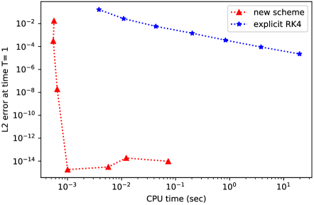
Figure 1: Convergence plot for the (BO) equation in $L^{2}$ against the computational cost at time $T=1$ for the exact solution (14) (with $c=\frac{15}{4\pi}$). Each point corresponds to a different value of $K$, ranging between $2^{3}$ and $2^{9}$. The new scheme in red is given in equation (1), the scheme in blue is the Fourier pseudo-spectral method coupled with a standard Runge-Kutta method (RK4).

We start by making a few remarks on Theorem 1.3. Our spectral rate coincides with those obtained in the literature when analyzing semi-discrete Fourier pseudo-spectral methods, see Deng–Ma [16] in the case of (BO) (with $r=1/2$, $s\geq 2$ ) and Maday–Quarteroni [39] in the case of the KdV equation (with $r=1$, $s>4$).

While the (BO) equation is globally well-posed for initial data $u_{0}\in H^{s}$ with $s>-1/2$, the above theorem only yields decay rates when $s>1$. It is the aim of a future project to consider low-regularity data with $s\leq 1$, by either considering different techniques for the proof or by employing a different method of approximation. For example [15] obtains sharper rates $K^{-s+r}$ for a spatial semi-discretization with a spectral Galerkin method (with $r=1/2$ and smooth enough solutions).

Lastly, note that the error constant $C$ in (2) depends only on $\|u_{0}\|_{H^{s}}$ and $\|u(t)\|_{H^{s}}$, instead of $\|u\|_{L^{\infty}([0,t],H^{s})}$, because we do not compute the solution at intermediate times, unlike any time-stepping method. In the case of (BO), we can bound $\|u\|_{L^{\infty}(\mathbb{R},H^{s})}$ as a function of $\|u_{0}\|_{H^{s}}$, independently of the final time $t$ [27, 34]. Hence, one could remove $\|u(t)\|_{H^{s}}$ from the statement of the theorem, up to a change in the constant $C$. The same also holds for (CS), by compactness of the orbit of the solution [4], except in the focusing case with critical and supercritical mass ($\|u\|_{L^{2}(\mathbb{T})}\geq 1$), which is why we choose to formulate the theorem in this manner, see Remark 5.10.

1.2 Outline

The rest of the article proceeds as follows. In Section 2 we set the scene and introduce the spaces and norms we work with throughout the article, together with bilinear estimates which are used in the proof of the main theorem. Section 3 contains the explicit formulas based on the Lax pair formulation. We derive our numerical schemes based on these formulas in Section 4 and discuss their computational cost and accuracy, comparing them with existing schemes in the literature. We give numerical experiments in Section 4.2, in the case of the Benjamin–Ono equation. After defining and establishing several tools crucial for the analysis in Section 5.1, we prove in Section 5.2 the spectral convergence result announced in Theorem 1.3.

Acknowledgements

The authors would like to deeply thank Patrick Gérard for stimulating discussions and constructive feedback. We also thank Rana Badreddine for helpful remarks, and for her PhD defence where this project was started. Y.A.B also thanks Louise Gassot for fruitful discussions on the Benjamin–Ono equation. The work of Y.A.B. is funded by the National Science Foundation through the award DMS-2401858 and M.D. acknowledges funding by the Deutsche Forschungsgemeinschaft (DFG, German Research Foundation) - Project number 442047500 through the Collaborative Research Center “Sparsity and Singular Structures” (SFB 1481).

2 Norms, spaces and Fourier transforms

Crucial for the analysis, and a common point of our three equations, is the space in which we study them. We define the Hardy space of functions whose Fourier transform is supported in $\mathbb{N}_{0}$ by

$$L^{2}_{+}=\{f\in L^{2}(\mathbb{T}):\widehat{f}(k)=0\ \text{for}\ k<0\},$$ (3)

where the $L^{2}$ inner product and the Fourier coefficients are respectively defined as

$$\langle f,g\rangle_{L^{2}}^{2}=\frac{1}{2\pi}\int_{-\pi}^{\pi}f(x)\overline{g(x)}dx\quad\text{and}\quad\widehat{f}(k)=\frac{1}{2\pi}\int_{-\pi}^{\pi}f(x)e^{-ikx}dx.$$

For concision, we use the shorthand notation $\|f\|=\|f\|_{L^{2}}$ and $\langle f,g\rangle=\langle f,g\rangle_{L^{2}}$. With these definitions, Fourier inversion, Parseval identity and the product-convolution identity read as follows:

$$f(x)=\sum_{k\in\mathbb{Z}}\widehat{f}(k)e^{ikx},\quad\|f\|_{L^{2}}^{2}=\sum_{k\in\mathbb{Z}}|\widehat{f}(k)|^{2}\quad\text{and}\quad\widehat{fg}=\widehat{f}*\widehat{g}.$$

By identifying $\mathbb{T}$ with the unit circle in $\mathbb{C}$, the space $L^{2}_{+}$ can equivalently be characterized as the traces of holomorphic functions $f$ on the unit disk

$$\mathbb{D}=\{z\in\mathbb{C}:|z|<1\},$$

satisfying

$$\sup_{r<1}\,\frac{1}{2\pi}\int_{-\pi}^{\pi}|f(re^{ix})|^{2}\,dx<+\infty.$$

The explicit formulas in the literature use this characterization, see equations (5), (7) and (9). We point out that the previously mentioned Riesz–Szegő operator ($\Pi$) is the orthogonal projector from $L^{2}$ to $L^{2}_{+}$.

For $r>0$, we also introduce the Sobolev space $H^{r}=\{f\in L^{2}:\|f\|_{H^{r}}<\infty\}$ with

$$\|f\|_{H^{r}}^{2}=\|(I+D^{2})^{r/2}f\big{\|}^{2}=\sum_{k\in\mathbb{Z}}(1+k^{2})^{r}|\widehat{f}(k)|^{2},$$

and the Hardy–Sobolev space

$$H^{r}_{+}=H^{r}\cap L^{2}_{+}.$$ (4)

We immediately see that, for $r^{\prime}<r$ and $f\in H^{r}$, $\|f\|_{H^{r^{\prime}}}\leq\|f\|_{H^{r}}$. Moreover, the following bilinear estimate holds:

Lemma 2.1.

Let $s>1/2$ and $0\leq\sigma\leq s$. Then, for all $f\in H^{s}$ and $g\in H^{\sigma}$,

$$\|fg\|_{H^{\sigma}}\leq C_{1}\|f\|_{H^{s}}\|g\|_{H^{\sigma}}.$$

The proof of the above lemma is quite standard, nevertheless we recall it in Section 6 for completeness and traceability of the constants.

3 Explicit formulas

We now present the explicit formulas from [22, 4, 24], written as inversion dynamical formulas defined inside the open unit disk, see equations (5), (7) and (9). We derive from these formulas a characterization of the Fourier coefficients $\widehat{u}(t,k)$ of the solution in terms of the initial data $u_{0}$ and the time $t$, see equations (6), (8), (10), and Remark 3.1. This later formulation is perfectly suited for approximating numerically, via a spectral discretization, as will be seen in Section 4.

Recalling the definition of the Riesz-Szegő projector $\Pi:L^{2}\rightarrow L^{2}_{+}$ from ($\Pi$) and (3), we introduce another crucial operator, $S^{*}:L^{2}_{+}\rightarrow L^{2}_{+}$, which removes the zero-th Fourier coefficient and shifts all positive frequencies by one

$$S^{*}f=\Pi(e^{-ix}f),\quad\text{i.e.}\quad\widehat{S^{*}f}(k)=\mathbbm{1}_{k\geq 0}\,\widehat{f}(k+1),\quad f\in L^{2}_{+}.$$

We are now ready to state the explicit formulas.

Benjamin–Ono. For (BO), it was discovered by Gérard [22, Theorem 4] that

$$\Pi u(t,z)=\left\langle\left(I-ze^{it}e^{2itL_{u_{0}}^{\text{BO}}}S^{*}\right)^{-1}\Pi u_{0},1\right\rangle,\quad\forall z\in\mathbb{D},$$ (5)

where the Lax operator $L_{u_{0}}^{\text{BO}}$ is the semi-bounded self-adjoint operator defined on $H^{1}_{+}$ by

$$L_{u_{0}}^{\text{BO}}f=Df-\Pi(u_{0}f).$$

By expanding formula (5) into a Neumann series in $z=re^{ix}$ and letting $r$ tend to $1$, we identify the Fourier coefficients of the solution

$$\widehat{u}(t,k)=\left\langle(e^{it}e^{2itL_{u_{0}}^{\text{BO}}}S^{*})^{k}\Pi u_{0},1\right\rangle,\quad k\geq 0.$$ (6)

We note that in the case $k<0$ we simply have $\widehat{u}(t,k)=\overline{\widehat{u}(t,-k)}$ since $u$ is real-valued.

We now comment on other explicit formulas existing in the literature. A precursor to the inversion formula (5) is the work of Gérard–Kappeler [26, Lemma 4.1] which considers finite gap initial conditions. An explicit formula on the real line $\mathbb{R}$ is obtained by Gérard [22, Theorem 6], and extended by the second author [14] to less regular initial data $u_{0}\in L^{2}(\mathbb{R})$. In the case of rational initial data, an explicit formula on the real line is given in [9], expressed as a ratio of determinants. A generalization of Gérard’s explicit formula (5) to the full hierarchy of (BO) is presented in Killip–Laurens–Vişan [34].

Calogero–Sutherland DNLS. Badreddine’s explicit formula for (CS) in the focusing [4, Proposition 2.6] and defocusing [4, Theorem 1.7] case is given by

$$u(t,z)=\left\langle\left(I-ze^{-it}e^{-2itL_{u_{0}}^{\text{CS}}}S^{*}\right)^{-1}u_{0},1\right\rangle,\quad\forall z\in\mathbb{D},$$ (7)

where the Lax operator $L_{u_{0}}^{\text{CS}}$ is the semi-bounded self-adjoint operator of domain $H^{1}_{+}$ given by

$$L_{u_{0}}^{\text{CS}}f=Df\mp u_{0}\Pi(\overline{u_{0}}f),$$

where the signs $-$ and $+$ correspond to the focusing case and the defocusing case, respectively. By the same procedure as above, we infer from formula (7) the following characterization

$$\widehat{u}(t,k)=\left\langle(e^{-it}e^{-2itL_{u_{0}}^{\text{CS}}}S^{*})^{k}u_{0},1\right\rangle,\quad k\geq 0.$$ (8)

We recall that the initial data belongs to a space $H^{s}_{+}$, defined by (4), hence $\widehat{u}(t,k)=0$ for $k<0$. We refer to Killip–Laurens–Vişan [33] for an explicit formula on the real line $\mathbb{R}$, and to Sun [46] for a matrix valued-extension.

Cubic Szegő. The explicit formula found by Gérard and Grellier [24, Theorem 1] reads

$$u(t,z)=\left\langle\left(I-ze^{-itH_{u_{0}}^{2}}e^{itK_{u_{0}}^{2}}S^{*}\right)^{-1}e^{-itH_{u_{0}}^{2}}u_{0},1\right\rangle,\quad\forall z\in\mathbb{D},$$ (9)

where the self-adjoint operators $H_{u_{0}}$ and $K_{u_{0}}$ defined on $L^{2}_{+}$ are given by

$$H_{u_{0}}(f)=\Pi(u_{0}\bar{f})\quad\text{and}\quad K_{u_{0}}^{2}f=H_{u_{0}}^{2}f-\langle f,u_{0}\rangle u_{0},\quad f\in L^{2}_{+}.$$

Once again, we infer from the above the characterization in Fourier

$$\widehat{u}(t,k)=\left\langle(e^{-itH_{u_{0}}^{2}}e^{itK_{u_{0}}^{2}}S^{*})^{k}e^{-itH_{u_{0}}^{2}}u_{0},1\right\rangle,\quad k\geq 0.$$ (10)

As for the (CS) equation, we have $\widehat{u}(t,k)=0$ for $k<0$.

An explicit formula was also derived for matrix valued extensions of (S) in Sun [47]. On $\mathbb{R}$, explicit formulas were found by Pocovnicu [42] and Gérard–Pushnitski [30].

Remark 3.1.

The characterization in Fourier (6) already appeared in [22, Remark 5] for (BO), and allowed to extend the explicit formula down to more singular initial data $u_{0}\in H^{s}$, with $s>-\frac{1}{2}$.

4 New schemes based on the explicit formulas

4.1 Construction of the schemes

In this section we present the three numerical schemes for the (BO), (CS) and (S) equations, derived from the explicit formulas (6), (8) and (10) respectively. We construct schemes of the general form (1), by restricting all operators to the $K$ frequencies $(0,\dots,K-1)$.

We discretize in $\mathbb{C}^{K\times K}$ the shift operator, the derivative and the convolution with $u_{0}$ as

$${\bf S}^{*}=(\mathbbm{1}_{k+1=\ell})_{0\leq k,\ell<K}\quad{\bf D}=(k\mathbbm{1}_{k=\ell})_{0\leq k,\ell<K}\quad\text{and}\quad{\bf T}_{u_{0}}=(\widehat{u_{0}}(k-\ell))_{0\leq k,\ell<K}.$$

Observe that for (BO), ${\bf T}_{u_{0}}$ is hermitian because $u_{0}$ is real-valued, while for (CS) it is lower triangular since $u_{0}\in L^{2}_{+}$.

Introducing the discretization ${\bf D}-{\bf T}_{u_{0}}$ of the Lax operator $L_{u_{0}}^{\text{BO}}$, the scheme for (BO) is obtained by taking

$${\bf A}={\bf I}+2{\bf D}-2{\bf T}_{u_{0}}\quad\text{and}\quad{\bf M}=0$$ (11)

in equation (1).

For (CS), we let ${\bf T}_{u_{0}}^{*}$ denote the conjugate transpose of ${\bf T}_{u_{0}}$, which corresponds to a convolution with $\overline{u_{0}}$. We similarly recover the scheme by taking

$${\bf A}={-\bf I}-2{\bf D}\pm 2{\bf T}_{u_{0}}{\bf T}_{u_{0}}^{*}\quad\text{and}\quad{\bf M}=0,$$ (12)

where the signs $+$ and $-$ correspond to the focusing case and the defocusing case, respectively.

Finally, for (S), to take into account the conjugation of the argument of $H_{u_{0}}$, we modify the convolution matrix as follows

$${\bf H}_{u_{0}}=(\widehat{u_{0}}(k+\ell))_{0\leq k,\ell<K}.$$

We then define the scheme through the choices

$${\bf A}={\bf H}_{u_{0}}{\bf H}_{u_{0}}^{*}-{\bf u}_{0}{\bf u}_{0}^{*}\quad\text{and}\quad{\bf M}={\bf H}_{u_{0}}{\bf H}_{u_{0}}^{*},$$ (13)

which are truncations of the operators $K_{u_{0}}^{2}$ and $H_{u_{0}}^{2}$, respectively.

The above schemes are computed entirely in Fourier space. To understand why this yields efficient algorithms, we need to consider their computational cost together with their precision. Namely, for our schemes (1) the accuracy $\epsilon=\|u(t)-u_{K}(t)\|$ and computational cost $\mathcal{C}$ are of order

$$\epsilon\sim TK^{-s+1}\quad\text{and}\quad\mathcal{C}\sim K^{3},$$

where $T=t$ is the final time and $K$ the number of frequencies in the discretization. We note that the leading cost comes from computing the matrix exponentials in equation (1). Thereby, the cost required to reach an accuracy $\epsilon$ is of order

$$\mathcal{C}\sim\left(\frac{T}{\epsilon}\right)^{\frac{3}{s-1}},$$

which for large $s$ beats fully-discrete schemes in the literature.

We make the important observation that the main reason why these new schemes are efficient is the fact that they are exact in time, hence the high precision compensates for the computational cost. On the other hand, any fully discrete method which involves coupling a time discretization with a fully spectral method, yields costly schemes with computational complexity in $O(K^{2})$ per time step. Hence, for practical purposes one resorts to pseudo-spectral methods in space, which rely on the Fast Fourier Transform (FFT) and its inverse to compute efficiently the nonlinearity. This yields algorithms whose cost per time step is $O(K\log K)$ instead of $O(K^{2})$. The resulting schemes $u^{n}_{{K}}$ have accuracy $\epsilon=\|u(n\tau)-u^{n}_{K}\|$ and computational effort $\mathcal{C}$ of order

$$\epsilon\sim e^{T}\left(\tau^{m}+K^{-s+1}\right)\quad\text{and}\quad\mathcal{C}\sim\frac{T}{\tau}K\log(K),$$

with $\tau$ the time step, $m\in\mathbb{N}$ the fixed order of the time approximation and $n$ the time iteration. We easily see that given the order $m$, and for smooth enough solutions, the error $\epsilon$ will be dominated by the time-approximation error $\tau^{m}$. Hence, the computational cost to obtain $\epsilon$ accuracy is much higher than that of our new schemes. The case of rougher solutions needs to be adressed separately, and will depend on the rate $m$ as a function of the regularity $s$, as well as on the CFL condition required by the low-regularity scheme. This analysis goes beyond the scope of this paper and will be given elsewhere.

Finally, our schemes are remarkably more efficient for simulating over long times, thanks to the fact that our error constant depends linearly on the final time $T$, instead of exponentially.

The above mentioned facts are witnessed in the numerical experiments of the next section.

Remark 4.1 (Different formulations of the scheme).

The above schemes are written in the form to be implemented. We can write the schemes – as is done in Section 5.1.2 for (BO) – in a more theoretical fashion using only the operator $\Pi_{K}$, which is better suited for analyzing their convergence.

4.2 Numerical results in the case of the Benjamin–Ono equation

We illustrate our numerical results using the $2\pi$-periodic travelling wave solutions

$$u^{*}(t,x)=\frac{1}{c-\sqrt{c^{2}-1}\cos(x-ct)},\quad c>1.$$ (14)

These travelling waves, obtained by Benjamin [7], were proved by Amick-Toland [3] to be unique. We note that when $c>1$, the solution $u^{*}$ is real and forms a single solitary wave. In the following we take either $c=\frac{15}{4\pi}$, in agreement with the example of [50], or $c=\frac{15}{\pi}$ which corresponds to a tighter peak.

While there is a vast literature on different numerical schemes for the (BO) equation, we choose to compare ours with the scheme consisting of coupling a Fourier pseudo-spectral method with a standard explicit 4-stage Runge-Kutta (RK4) time-stepping method. Although, up to our knowledge, no convergence results exists for this scheme, it remains a very popular method to obtain a high order approximation of smooth solutions, see for example [11]. To ensure stability of the method we impose a CFL condition of the form $\tau\leq Ch^{2}$, where $h=\frac{2\pi}{K}$ is the spatial mesh size. In the following numerical simulations we take $C=\frac{1}{4}$.

As previously mentioned, this pseudo-spectral method has a computational cost in $\frac{T}{\tau}K\log(K)$ when computing up until the final time $T$. Given the quadratic CFL condition the cost of the pseudo-spectral RK4 method is of order $TK^{3}\log K$. This is to be compared with the cost of the new scheme (1) which is of order $K^{3}$.

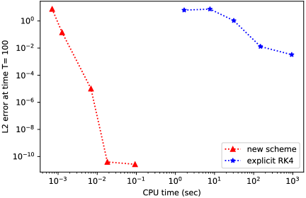
Figure 2: Convergence plot for the (BO) equation in $L^{2}$ against the computational cost up to time $T=100$ for the exact solution (14) (with $c=\frac{15}{\pi}$). We choose the number of Fourier modes $K$ to be powers of two ranging from 32 to 512.

We show in numerical simulations how the new scheme (1) clearly outperforms previous schemes in the literature, both in the case of short (Figure 1) and long (Figures 2, 3) times, and compare it with the pseudo-spectral RK4 scheme. In Figure 1 and 2 we chose as final times $T=1$ and $T=100$ respectively, and compute the CPU-time versus $L^{2}$-error of the scheme for varying time and space step sizes. We see that the new scheme is far more precise. This is thanks to the fact that it is exact in time, with spectral accuracy in space, hence the error decreases faster than any polynomial. In contrast, for smooth solutions, the error of any fully discrete pseudo-spectral scheme existing in the literature is dominated by the time discretization error of order $\tau^{m}$, for some fixed $m\in\mathbb{N}$, which hence induces a larger error. Our schemes also perform well for large times since the error constant only grows linearly in time, see Theorem 1.3. This is not the case of classical methods in the literature whose error constant grows exponentially in the final time $T$, and hence can yield poor results over long times. We refer to Figure 3 where the exact periodic solution and numerical approximations are plotted at time $t=500$, we see that only the new scheme gives a reliable approximation. The CPU times needed to compute these schemes is $215$ s for the RK4 method versus $6.28\times 10^{-3}$ s for the new scheme.

Having motivated in numerical simulations the advantages of the new scheme (1), we now prepare the ground for proving its convergence and introduce in the following section some notations and definition of operators used in the proof.

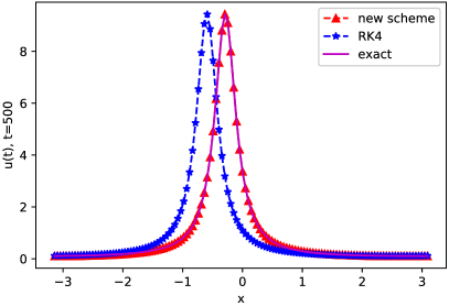
Figure 3: Plot of the solution (14) in purple (with $c=\frac{15}{\pi}$), the new scheme (1) in red, and the pseudo-spectral RK4 method in blue. We choose $t=500$ and $K=128$. The initial profile is translated at constant speed $c$, thus it has periodically returned near the origin $ct/2\pi\approx 380$ times between $0$ and $t$.

5 Proving convergence

We recall that in this section we consider the (BO) equation, whose solution and initial data are real-valued functions.

5.1 Prerequisites for the proof

5.1.1 The Lax Pair

Given $u\in H^{2}$, we can define the following Toeplitz operator on $L_{+}^{2}$,

$$\forall f\in L_{+}^{2},\quad T_{u}f=\Pi(uf).$$

With the above notation, we recall the Lax operator $L_{u}$ for (BO) already introduced in Section 3,

$$L_{u}=D-T_{u}.$$

In the proof, we will use the second Lax operator $B_{u}$, which is a bounded skew-adjoint operator defined by

$$B_{u}=i\left(T_{|D|u}-T_{u}^{2}\right),$$ (15)

as well as the following two propositions whose proofs are given in [22].

Proposition 5.1.

[22, Corollary 3] Let $u(t)$ be the solution of (BO) with initial data $u_{0}\in H^{2}$. Denote by $U(t)$ the operator-valued solution of the linear ODE

$$U^{\prime}(t)=B_{u(t)}U(t),\quad U(0)=I.$$

Then for every $t\in\mathbb{R}$, $U(t)$ is unitary on $L_{+}^{2}$, and

$$L_{u(t)}=U(t)L_{u_{0}}U(t)^{*}.$$

During the derivation of the explicit formula in [22, Section 2], at the bottom of page 597, Gérard discovered the following identity.

Proposition 5.2.

Under the condition of Lemma 5.1, we have

$$U(t)^{*}S^{*}U(t)=e^{it\left(L_{u_{0}}+I\right)^{2}}S^{*}e^{-itL_{u_{0}}^{2}}.$$

Remark 5.3.

The operator $U(t)$ can be shown to be unitary on $L^{2}_{+}$ for $u(t)\in H^{s}$, $s>3/2$. Indeed, the regularity requirement stems from equation (15) where a standard bilinear estimate requires $|D|u\in L^{\infty}$. Hence, the above two lemmas can be stated for $u(t)$ in these weaker spaces. Nevertheless, to be consistent with prior works we keep the stronger hypothesis $u(t)\in H^{2}$, as this does not change the steps in our proof which follow by density for $s<2$.

5.1.2 Truncated Lax operator

Recalling the definition oh $\Pi_{K}$ from Section 1.1, we define the operator $L_{u_{0},K}$ by

$$L_{u_{0},K}f=Df-\Pi_{K}(u_{0}\Pi_{K}f),\quad f\in L^{2}_{+},$$

and let

$$A=I+2L_{u_{0}}\quad\text{and}\quad A_{K}=I+2L_{u_{0},K}.$$

According to equations (6) and (1), it follows that for $k\in\{0,\dots,K-1\}$,

$$\widehat{u}(t,k)=\langle(e^{itA}S^{*})^{k}\Pi u_{0},1\rangle\quad\text{and}\quad\widehat{u_{K}}(t,k)=\langle(e^{itA_{K}}S^{*})^{k}\Pi_{K}u_{0},1\rangle.$$

Remark 5.4.

In the computation of $u_{K}$, we only apply $e^{itA_{K}}$ to functions $f$ in

$$L^{2}_{K}=\Big{\{}f\in L^{2},\;\operatorname{supp}(\widehat{f})\subset\{0,\dots,K-1\}\Big{\}},$$

for which $L_{u_{0},K}f=Df-\Pi_{K}(u_{0}f)$. However, we need a second $\Pi_{K}$ in the definition in order to make $L_{u_{0},K}$ self-adjoint on $L^{2}_{+}$.

With the above definitions, the operators $e^{itA}$ and $e^{itA_{K}}$ preserve the $L^{2}$ norm.

Lemma 5.5.

For any $f\in L^{2}_{+}$, $\|e^{itA_{K}}f\|_{L^{2}}=\|f\|_{L^{2}}$ and $\|e^{itA}f\|_{L^{2}}=\|f\|_{L^{2}}$.

Proof.

For $f,g\in L^{2}_{+}$, as $u_{0}$ is real-valued,

$$\langle\Pi_{K}(u_{0}\Pi_{K}f),g\rangle=\langle u_{0}\Pi_{K}f,\Pi_{K}g\rangle=\langle\Pi_{K}f,u_{0}\Pi_{K}g\rangle=\langle f,\Pi_{K}(u_{0}\Pi_{K}g)\rangle$$

and

$$\langle Df,g\rangle=\sum_{k\geq 0}k\widehat{f}(k)\overline{\widehat{g}(k)}=\langle f,Dg\rangle.$$

Therefore $L_{u_{0},K}$ is self-adjoint, and so is $A_{K}$. As a consequence,

$$\frac{d}{dt}\|e^{itA_{K}}f\|_{L^{2}}^{2}=\langle(iA_{K}-iA_{K}^{*})e^{itA_{K}}f,e^{itA_{K}}f\rangle=0,$$

and the first equality follows by integrating the last equation between $0$ and $t$. The second one is obtained in a similar fashion, by replacing $\Pi_{K}$, $L_{u_{0},K}$ and $A_{K}$ by $\Pi$, $L_{u_{0}}$ and $A$, respectively. ∎

5.1.3 Equivalent norms

In the next lemmas, we assume that $t$, $s$ and $u_{0}$ are fixed. The constants $C_{i}$ are allowed to depend on $s$, $\|u_{0}\|_{H^{s}}$, $\|u(t)\|_{H^{s}}$, and $C_{j}$ for $j<i$. Let $C_{2}=C_{1}\max(\|u_{0}\|_{H^{s}},\|u(t)\|_{H^{s}})+1$ and $C_{3}=2C_{2}$. The following equivalence of norms holds for $m=\lceil s\rceil$.

Lemma 5.6.

For $u\in\{u_{0},u(t)\}$ and $f\in H^{m}_{+}$ with $m=\lceil s\rceil$, it holds

$$C_{3}^{-m}\|f\|_{H^{m}}\leq\|(L_{u}+C_{2}I)^{m}f\|\leq C_{3}^{m}\|f\|_{H^{m}}.$$

Proof.

For any $n\in\{0,\dots,m\}$, denote

$$f_{n}=(L_{u}+C_{2}I)^{m-n}f.$$

For $n<m$ and $g\in H^{n+1}$, Lemma 2.1 shows that $\|ug\|_{H^{n}}\leq(C_{2}-1)\|g\|_{H^{n}}$, and hence

$$\|(L_{u}+C_{2}I)g\|_{H^{n}}\leq\|Dg\|_{H^{n}}+\|ug\|_{H^{n}}+C_{2}\|g\|_{H^{n}}\leq 2C_{2}\|g\|_{H^{n+1}}.$$

In particular,

$$\|f_{n}\|_{H^{n}}\leq C_{3}\|f_{n+1}\|_{H^{n+1}},$$

which proves the upper bound $\|f_{0}\|\leq C_{3}^{m}\|f_{m}\|_{H^{m}}$ by induction.

For the lower bound, we first note that for any $g\in H^{n+1}_{+}$,

$$\langle(L_{u}+(C_{2}-1)I)g,g\rangle_{H^{n}}=\langle Dg,g\rangle_{H^{n}}-\langle ug,g\rangle_{H^{n}}+(C_{2}-1)\|g\|_{H^{n}}^{2}\geq 0,$$

hence

$$\|(L_{u}+C_{2}I)g\|_{H^{n}}^{2}=\|(L_{u}+(C_{2}-1)I)g\|_{H^{n}}^{2}+2\langle(L_{u}+(C_{2}-1)I)g,g\rangle_{H^{n}}+\|g\|_{H^{n}}^{2}\geq\|g\|_{H^{n}}^{2}.$$

From this, we obtain

$$\|g\|_{H^{n+1}}\leq\|(D+I)g\|_{H^{n}}\leq\|(L_{u}+C_{2}I)g\|_{H^{n}}+\|ug\|_{H^{n}}+(C_{2}-1)\|g\|_{H^{n}}\leq 2C_{2}\|(L_{u}+C_{2}I)g\|_{H^{n}},$$

and we conclude again by induction on $\|f_{n}\|_{H^{n}}$. ∎

5.2 The proof of convergence

In this section we prove Theorem 1.3. We summarize in the following sentences the sequence of steps needed to complete the proof, which differs very much from classical techniques to show convergence of schemes (by coupling a local error and stability bound). It requires a deep understanding of the Lax pairs, their commutation properties with the shift operator $S^{*}$ on the Hardy space $L^{2}_{+}$, and of the explicit form of the solution (5). Indeed, while the error committed by the projection $\Pi-\Pi_{K}$ is trivially of order $O(K^{-s})$, the error made my discretizing the Lax operator $L_{u_{0}}$, and hence the term $(e^{itA}S^{*})^{k}-(e^{itA_{K}}S^{*})^{k}$, is much harder to control. In order to buckle the proof we first bound, in Lemma 5.7, the error of approximation of the linear flow $e^{itA}$. The bound involves the $H^{s}$ norm of a function $u^{k}$ related to the solution $u$, which needs to be controlled. This is done in Lemma 5.8, which is the most technical part of the proof and calls upon the second Lax operator $B_{u}$, the identities introduced in Section 5.1.1, and the equivalence of norms in Section 5.1.3. The proof of the theorem is then shown by proceeding by induction on the Fourier coefficients, without Gronwall-type argument, and thereby allows to obtain a global bound with a linear dependence on the final time $t$.

Lemma 5.7.

For $f\in L^{2}_{+}$ and $s>1/2$,

$$\|e^{itA}f-e^{itA_{K}}f\|\leq 4C_{1}\|u_{0}\|_{H^{s}}\,t\,K^{-s}\sup_{t^{\prime}\in[0,t]}\|e^{it^{\prime}A}f\|_{H^{s}}.$$

Proof.

We let

$$F(t^{\prime})=e^{i(t-t^{\prime})A_{K}}e^{it^{\prime}A}f,$$

and observe that

$$\|e^{itA}f-e^{itA_{K}}f\| =\|F(t)-F(0)\|=\left\|\int_{0}^{t}\frac{dF}{dt^{\prime}}dt^{\prime}\right\|$$

$$\leq\int_{0}^{t}\|e^{i(t-t^{\prime})A_{K}}(A_{K}-A)e^{it^{\prime}A}f\|dt^{\prime}$$

$$=\int_{0}^{t}\|(A_{K}-A)e^{it^{\prime}A}f\|dt^{\prime},$$

where we used Lemma 5.5 in the last equality. For $g=e^{it^{\prime}A}f$, we have

$$\frac{1}{2}(A_{K}-A)g=\Pi(u_{0}g)-\Pi_{K}(u_{0}\Pi_{K}g)=(\Pi-\Pi_{K})(u_{0}g)-\Pi_{K}(u_{0}(g-\Pi_{K}g)),$$

so we conclude with

$$\|(A_{K}-A)g\| \leq 2\|(\Pi-\Pi_{K})(u_{0}g)\|+2\|\Pi_{K}(u_{0}(g-\Pi_{K}g))\|$$

$$\leq 2\|u_{0}g\|_{H^{s}}K^{-s}+2C_{1}\|u_{0}\|_{H^{s}}\|g-\Pi_{K}g\|$$

$$\leq 4C_{1}\|u_{0}\|_{H^{s}}\|g\|_{H^{s}}K^{-s},$$

with the constant $C_{1}$ from Lemma 2.1. ∎

Lemma 5.8.

Given any integer $k\geq 0$, let $u^{k}=(e^{itA}S^{*})^{k}\Pi u_{0}$. Then for any $\tilde{t}\in[0,t]$,

$$\|e^{-i\tilde{t}A}u^{k}\|_{H^{s}}\leq C_{3}^{4s}\|u_{0}\|_{H^{s}}.$$

Proof.

We first assume that $u_{0}\in H^{2}$, in order to ensure that $B_{u(t)}$ and $U(t)$ are well-defined. By definition of $A$ and Proposition 5.2, we have

$$e^{itA}S^{*}=e^{it+2itL_{u_{0}}}S^{*}=e^{-itL_{u_{0}}^{2}}e^{it\left(L_{u_{0}}+I\right)^{2}}S^{*}=e^{-itL_{u_{0}}^{2}}U(t)^{*}S^{*}U(t)e^{itL_{u_{0}}^{2}}.$$

By induction, we thereby obtain

$$(e^{itA}S^{*})^{k}=e^{-itL_{u_{0}}^{2}}U(t)^{*}(S^{*})^{k}U(t)e^{itL_{u_{0}}^{2}},$$

so $e^{-i\tilde{t}A}u^{k}=P(S^{*})^{k}Q\Pi u_{0}$, with

$$P=e^{-i\tilde{t}A}e^{-itL_{u_{0}}^{2}}U(t)^{*}\quad\text{and}\quad Q=U(t)e^{itL_{u_{0}}^{2}}.$$

As $A$ and $L_{u_{0}}$ are self-adjoint, and $U(t)$ is unitary, for any $f\in L^{2}_{+}$,

$$\|Pf\|=\|Qf\|=\|f\|.$$

Moreover, by Lemma 5.6 and Proposition 5.1, for any $f\in H^{m}_{+}$ with $m=\lceil s\rceil$,

$$\|Pf\|_{H^{m}}\leq C_{3}^{m}\|(L_{u_{0}}+C_{2}I)^{m}Pf\|=C_{3}^{m}\|P(L_{u(t)}+C_{2}I)^{m}f\|=C_{3}^{m}\|(L_{u(t)}+C_{2}I)^{m}f\|\leq C_{3}^{2m}\|f\|_{H^{m}}.$$

As $P$ is unitary, $P^{-1}=P^{*}$ is also bounded in $H^{m}$. According to Lemma 6.2,

$$\|P\|_{H^{s}\to H^{s}}\leq\|P\|_{L^{2}\to L^{2}}^{(m-s)/m}\,\|P\|_{H^{m}\to H^{m}}^{s/m}\leq C_{3}^{2s}.$$

Proceeding in the same way with $Q$, we obtain

$$\|e^{-i\tilde{t}A}u^{k}\|_{H^{s}}\leq C_{3}^{2s}\|(S^{*})^{k}Q\Pi u_{0}\|_{H^{s}}\leq C_{3}^{2s}\|Q\Pi u_{0}\|_{H^{s}}\leq C_{3}^{4s}\|\Pi u_{0}\|_{H^{s}}\leq C_{3}^{4s}\|u_{0}\|_{H^{s}}.$$

For $u_{0}\in H^{s}$ with $1<s<2$, we can take a sequence $(u_{0}^{n})_{n\in\mathbb{N}}\in(H^{2})^{\mathbb{N}}$ that approximates $u_{0}$ in $H^{s}$. By the continuity of the flow map [40, Theorem 1.1], we have $u^{n}(t)\underset{n\rightarrow\infty}{\longrightarrow}u(t)$ in $H^{s}$. Moreover, defining $A^{n}=I+2L_{u_{0}^{n}}$ and following the proof of Lemma 5.7 we have that for every $v\in H_{+}^{s}$,

$$\|e^{itA^{n}}v-e^{itA}v\|_{H^{s}} \leq 2\int_{0}^{t}\|e^{i(t-t^{\prime})A^{n}}(T_{u_{0}^{n}}-T_{u_{0}})e^{it^{\prime}A}v\|_{H^{s}}dt^{\prime}$$

$$\leq 2\,C_{3}^{2s}\int_{0}^{t}\|(T_{u_{0}^{n}}-T_{u_{0}})e^{it^{\prime}A}v\|_{H^{s}}dt^{\prime}$$

$$\leq 2\,C_{1}\,C_{3}^{4s}\,t\,\|u_{0}^{n}-u_{0}\|_{H^{s}}\|v\|_{H^{s}}\underset{n\rightarrow\infty}{\longrightarrow}0.$$

Hence, for fixed $t$ we have $e^{itA^{n}}\underset{n\rightarrow\infty}{\longrightarrow}e^{itA}$ in $\mathcal{L}(H_{+}^{s})$ (norm topology), and by applying an induction argument we obtain the convergence

$$e^{-i\tilde{t}A^{n}}(e^{itA^{n}}S^{*})^{k}\Pi u_{0}^{n}\underset{n\rightarrow\infty}{\longrightarrow}e^{-i\tilde{t}A}(e^{itA}S^{*})^{k}\Pi u_{0},\quad\text{in}\ H_{+}^{s}.$$

By following the above proof with $u_{0}$ replaced by $u_{0}^{n}$, we have

$$\|e^{-i\tilde{t}A^{n}}(e^{itA^{n}}S^{*})^{k}\Pi u_{0}^{n}\|_{H^{s}}\leq(2C_{1}\max(\|u_{0}^{n}\|_{H^{s}},\|u^{n}(t)\|_{H^{s}})+2)^{4s}\|u_{0}^{n}\|_{H^{s}}.$$

Therefore, by taking the limit as $n\rightarrow\infty$ in the above, we recover the desired bound by $C_{3}^{4s}\|u_{0}\|_{H^{s}}$ also in the case $1<s<2$, which completes the proof. ∎

Proof of Theorem 1.3.

We recall that for notational convenience, we write $\|\cdot\|=\|\cdot\|_{L^{2}}$. For $k\geq 0$, denote

$$v^{k}=(e^{itA}S^{*})^{k}\Pi u_{0}-(e^{itA_{K}}S^{*})^{k}\Pi_{K}u_{0},\quad\text{and}\quad w^{k}=e^{itA_{K}}S^{*}v^{k}.$$

Notice that the Fourier coefficients of the error satisfy, for $k\in\{0,\dots,K-1\}$,

$$e_{k}:=\widehat{u}(t,k)-\widehat{u_{K}}(t,k)=\langle(e^{itA}S^{*})^{k}\Pi u_{0},1\rangle-\langle(e^{itA_{K}}S^{*})^{k}\Pi_{K}u_{0},1\rangle=\langle v^{k},1\rangle.$$

Using the property of the shift operator $S^{*}$ and Lemma 5.5 thus yields

$$\|v^{k}\|^{2}=|\langle v^{k},1\rangle|^{2}+\|S^{*}v^{k}\|^{2}=|e_{k}|^{2}+\|w^{k}\|^{2}.$$ (16)

Moreover, recalling that $u^{k}=(e^{itA}S^{*})^{k}\Pi u_{0}$ and defining

$$\varepsilon^{k}=(e^{itA}-e^{itA_{K}})S^{*}u^{k},$$

we have

$$v^{k+1}=w^{k}+\varepsilon^{k}.$$ (17)

For $C_{4}=4\,C_{1}\|u_{0}\|_{H^{s}}^{2}C_{3}^{4s}$, we can bound

$$\|\varepsilon^{k}\|=\|(e^{itA}-e^{itA_{K}})e^{-itA}u^{k+1}\|\leq 4C_{1}\|u_{0}\|_{H^{s}}tK^{-s}\sup_{t^{\prime}\in[0,t]}\|e^{i(t^{\prime}-t)A}u^{k+1}\|_{H^{s}}\leq C_{4}\,t\,K^{-s},$$

where we used Lemma 5.7 in the first inequality, and Lemma 5.8 in the second.

Applying successively (17) and (16), we see that

$$\|v^{k+1}\|\leq\|w^{k}\|+\|\varepsilon^{k}\|\leq\|v^{k}\|+\|\varepsilon^{k}\|.$$

By induction, this implies that for all $k\geq 0$,

$$\|v^{k}\|\leq\|v^{0}\|+\sum_{\ell=0}^{k-1}\|\varepsilon^{\ell}\|\leq(\|u_{0}\|_{H^{s}}+C_{4}\,t\,k)K^{-s}.$$

Applying (16) and (17) one more time yields

$$\sum_{k=0}^{K-1}|e_{k}|^{2} =\sum_{k=0}^{K-1}\|v^{k}\|^{2}-\|w^{k}\|^{2}$$

$$\leq\|v^{0}\|^{2}+\sum_{k=0}^{K-1}\|v^{k+1}\|^{2}-\|w^{k}\|^{2}$$

$$=\|v^{0}\|^{2}+\sum_{k=0}^{K-1}(\|v^{k+1}\|+\|w^{k}\|)(\|v^{k+1}\|-\|w^{k}\|)$$

$$\leq\|v^{0}\|^{2}+\sum_{k=0}^{K-1}(\|v^{k+1}\|+\|v^{k}\|)\|\varepsilon^{k}\|$$

$$\leq\|u_{0}\|_{H^{s}}^{2}K^{-2s}+2\sum_{k=0}^{K-1}(\|u_{0}\|_{H^{s}}+C_{4}\,t\,K)\,C_{4}\,t\,K^{-2s}.$$

As the coefficients with negative indices are just complex conjugates, we conclude that for $0\leq r\leq s$,

$$\|u-u_{K}\|_{H^{r}}^{2} \leq 2\sum_{k\geq 0}(1+k^{2})^{r}|\widehat{u}(k)-\widehat{u_{K}}(k)|^{2}$$

$$\leq 2K^{2r}\sum_{k=0}^{K-1}|e_{k}|^{2}+\sum_{k\geq K}(1+k^{2})^{r}|\widehat{u}(k)|^{2}$$

$$\leq C_{5}^{2}(1+tK)^{2}K^{2r-2s},$$

with $C_{5}=2\|u_{0}\|_{H^{s}}+2C_{4}\leq 2^{8(s+1)^{2}}\max(\|u_{0}\|_{H^{s}},\|u(t)\|_{H^{s}},1)^{4s+1}\|u_{0}\|_{H^{s}}$. ∎

Remark 5.9.

The final result is actually slightly better than stated in Theorem 1.3, since we achieve the optimal decay rate $K^{-s+r}$ for small times $t=\mathcal{O}(K^{-1})$. For small initial data, it is also readily seen that $C_{5}$ tends to $0$ linearly with $\|u_{0}\|_{H^{s}}$.

Remark 5.10.

The analogue of Proposition 5.1 and Proposition 5.2 for the (CS) equation is obtained in [4, Equation 2-11 and 2-14]. By applying the same steps as in the proof of Theorem 1.3 one recovers the convergence rate of Theorem 1.3 for the scheme in equation (1) which approximates the (CS) equation. However, this result cannot be applied globally in time to the focusing case with critical or supercritical mass ($\|u\|_{L^{2}(\mathbb{T})}\geq 1$), as the global existence of the solution in such cases is not yet known.

6 Appendix

Proof of Lemma 2.1.

A proof on more general Sobolev spaces can be found in [2, Theorem 4.39], here we present a much simpler argument in $H^{s}$.

For $k,\ell\in\mathbb{Z}$, denoting $\langle k\rangle=\sqrt{1+k^{2}}$, it holds $\langle k\rangle^{\sigma}\leq 2^{\sigma}(\langle\ell\rangle^{\sigma}+\langle k-\ell\rangle^{\sigma})$. Letting $\mathcal{D}=(1+D^{2})^{\sigma/2}$, this yields

$$\Big{|}\widehat{\mathcal{D}(fg)}(k)\Big{|}=\langle k\rangle^{\sigma}\Big{|}\widehat{fg}(k)\Big{|}=\langle k\rangle^{\sigma}\Big{|}\sum_{\ell\in\mathbb{Z}}\widehat{f}(\ell)\,\widehat{g}(k-\ell)\Big{|} \leq 2^{\sigma}\Big{(}\widehat{\mathcal{D}f}*\widehat{g}+\widehat{f}*\widehat{\mathcal{D}g}\Big{)}(k).$$

By Young’s convolution inequality, for $p=\frac{2s}{2s-\sigma}$ and $q=\frac{2s}{s+\sigma}$, as $\frac{1}{p}+\frac{1}{q}=1+\frac{1}{2}$,

$$\big{\|}\mathcal{D}(fg)\big{\|}=\big{\|}\widehat{\mathcal{D}(fg)}\big{\|}_{2}\leq 2^{\sigma}\left(\big{\|}\widehat{\mathcal{D}f}\big{\|}_{p}\big{\|}\widehat{g}\big{\|}_{q}+\big{\|}\widehat{f}\big{\|}_{1}\big{\|}\widehat{\mathcal{D}g}\big{\|}_{2}\right).$$

Applying Hölder’s inequality with exponents $\frac{2}{2-p}$ and $\frac{2}{p}$,

$$\big{\|}\widehat{\mathcal{D}f}\big{\|}_{p}^{p}=\sum_{k\in\mathbb{Z}}\langle k\rangle^{\sigma p}|\widehat{f}(k)|^{p}\leq C_{0}^{\frac{2-p}{2}}\Big{(}\sum_{k\in\mathbb{Z}}\langle k\rangle^{2s}|\widehat{f}(k)|^{2}\Big{)}^{\frac{p}{2}}=C_{0}^{\frac{2-p}{2}}\|f\|_{H^{s}}^{p},$$

where $C_{0}=\sum_{k\in\mathbb{Z}}\langle k\rangle^{-2s}.$ By Hölder’s inequality with exponents $\frac{2}{2-q}$ and $\frac{2}{q}$, and Cauchy-Schwarz inequality, we also have

$$\big{\|}\widehat{g}\big{\|}_{q}^{q}\leq C_{0}^{\frac{2-q}{2}}\|g\|_{H^{\sigma}}^{q}\quad\text{and}\quad\|\widehat{f}\|_{1}\leq C_{0}^{\frac{1}{2}}\|g\|_{H^{s}}.$$

Finally, as $\big{\|}\widehat{\mathcal{D}g}\big{\|}_{2}=\|f\|_{H^{\sigma}}$, taking $C_{1}=2^{s+1}\sqrt{C_{0}}$, we conclude with

$$\big{\|}\mathcal{D}(fg)\big{\|}\leq 2^{\sigma}\Big{(}C_{0}^{\frac{1}{p}-\frac{1}{2}}C_{0}^{\frac{1}{q}-\frac{1}{2}}+C_{0}^{\frac{1}{2}}\Big{)}\|f\|_{H^{s}}\|g\|_{H^{\sigma}}\leq C_{1}\|f\|_{H^{s}}\|g\|_{H^{\sigma}}.$$

∎

Remark 6.1.

In the proof of the theorem, as $s>1$, we use the bound $C_{0}\leq\sum_{k\in\mathbb{Z}}\frac{1}{1+k^{2}}\leq 4$, and thus $C_{1}\leq 2^{s+2}$.

Lemma 6.2.

If $P$ is invertible in $H^{m}_{+}$ with $\|P\|_{L^{2}\to L^{2}}\leq 1$ and $\|P\|_{H^{m}\to H^{m}}\leq C_{3}^{2m}$, then

$$\|P\|_{H^{s}\to H^{s}}\leq C_{3}^{2s}.$$

Proof.

We use a simple version of $K$ interpolation. A general proof can be found in [2, Theorem 7.23]. For $f\in H^{s}$, define

$$K(t,f) :=\inf_{g\in H^{m}}\|f-g\|^{2}+t\|g\|_{H^{m}}^{2}$$

$$=\sum_{k\geq 0}\,\min_{\widehat{g}_{k}\in\mathbb{C}}\,|\widehat{f}_{k}-\widehat{g}_{k}|^{2}+t\langle k\rangle^{2m}|\widehat{g}_{k}|^{2}$$

$$=\sum_{k\geq 0}|\widehat{f}_{k}|^{2}\min_{\lambda\in[0,1]}(1-\lambda)^{2}+t\langle k\rangle^{2m}\lambda^{2}$$

$$=\sum_{k\geq 0}|\widehat{f}_{k}|^{2}\frac{t\langle k\rangle^{2m}}{1+t\langle k\rangle^{2m}}.$$

Observing that

$$\int_{0}^{\infty}\frac{t\langle k\rangle^{2m}}{1+t\langle k\rangle^{2m}}\,\frac{dt}{t^{1+s/m}}=\langle k\rangle^{2s}\int_{0}^{\infty}\frac{x^{-s/m}}{1+x}\,dx=C_{s}\langle k\rangle^{2s},$$

where $C_{s}$ only depends on $s$, we obtain

$$\|f\|_{H^{s}}^{2}=\frac{1}{C_{s}}\int_{0}^{\infty}K(t,f)\,\frac{dt}{t^{1+s/m}}.$$

Finally, as $P$ is invertible in $H^{m}_{+}$,

$$K(t,Pf)=\inf_{g\in H^{m}_{+}}\|Pf-Pg\|^{2}+t\|Pg\|_{H^{m}}^{2}\leq\inf_{g\in H^{m}_{+}}\|f-g\|^{2}+C_{3}^{4m}t\|g\|_{H^{m}}^{2}=K(C_{3}^{4m}t,f),$$

and therefore

$$\|Pf\|_{H^{s}}^{2}=\frac{1}{C_{s}}\int_{0}^{\infty}K(t,Pf)\,t^{-\frac{s}{m}}\,\frac{dt}{t}\leq C_{3}^{4s}\|f\|_{H^{s}}^{2}.$$

∎

References

- [1] G. Abanov, E. Bettelheim, P. Wiegmann, Integrable hydrodynamics of Calogero–Sutherland model: bidirectional Benjamin–Ono equation, J. Phys. A 42 (2009), no.13, pp.135201.
- [2] R. Adams, J.J.F. Fournier, Sobolev Spaces, Springer, 2003.
- [3] C. Amick, J. Toland, Uniqueness and related analytic properties for the Benjamin-Ono equation a nonlinear Neumann problem in the plane, Acta Math., 167(1991), 107–126.
- [4] R. Badreddine, On the global well-posedness of the Calogero–Sutherland derivative nonlinear Schrödinger equation, Pure and Applied analysis, 6(2) :3799414, 2024. doi:10.2140/paa.2024.6.379.
- [5] R. Badreddine, Traveling waves and finite gap potentials for the Calogero–Sutherland derivative nonlinear Schrödinger equation, Ann. Inst. H. Poincaré C Anal. Non Linéaire (2024).
- [6] R. Badreddine, Zero dispersion limit of the Calogero-Moser derivative NLS equation, SIAM Journal on Mathematical Analysis, 56(6), 7228-7249.
- [7] T. Benjamin, Internal waves of permanent form in fluids of great depth, J. Fluid Mech., 29(1967), 559–592.
- [8] A. Biasi, O. Evnin, Turbulent cascades in a truncation of the cubic Szegő equation and related systems, Analysis & PDE, 15(1), 217-243, 2022.
- [9] E. Blackstone, L. Gassot, P. Gérard, P. D. Miller, The Benjamin–Ono Initial-Value Problem for Rational Data, arxiv.org/abs/2410.14870, 2024.
- [10] E. Blackstone, L. Gassot, P. Gérard, P. D. Miller, The Benjamin–Ono equation in the zero-dispersion limit for rational initial data: generation of dispersive shock waves, arxiv.org/abs/2410.17405, 2024.
- [11] J.P. Boyd, Z. Xu, Comparison of three spectral methods for the Benjamin–Ono equation: Fourier pseudo-spectral, rational Christov functions and Gaussian radial basis functions, Wave Motion 48, 702–706 (2011)
- [12] F. Calogero, Solution of the one-dimensional N-body problems with quadratic and/or inversely quadratic pair potentials, Jour. of Math. Phys. 12 no. 3 (1971): 419–436.
- [13] R. Carles, C. Su. Scattering and uniform in time error estimates for splitting method in NLS, Found. Comput. Math. 24 (2024), 683–722.
- [14] X. Chen, Explicit formula for the Benjamin–Ono equation with square integrable and real valued initial data and applications to the zero dispersion limit, arXiv: 2402.12898, 2024. To appear in Pure and Applied Analysis.
- [15] Z. Deng, H. Ma, Optimal error estimates of the Fourier spectral method for a class of nonlocal, nonlinear dispersive wave equations. Appl. Numer. Math. 59, 988–1010 (2009)
- [16] Z. Deng, H. Ma, Error estimate of the Fourier collocation method for the Benjamin–Ono equation. Numer. Math. Theor. Meth. Appl, 2(341-352), 1 (2009).
- [17] R. Dutta, H. Holden, U. Koley, N.H. Risebro, Convergence of finite difference schemes for the Benjamin–Ono equation. Numer. Math. 134, 249–274 (2016).
- [18] M. Dwivedi, T. Sarkar, A Local discontinuous Galerkin method for the Benjamin–Ono equation. arXiv preprint arXiv:2405.08360 (2024).
- [19] S. T. Galtung, Convergence rates of a fully discrete Galerkin scheme for the Benjamin–Ono equation, XVI International Conference on Hyperbolic Problems: Theory, Numerics, Applications. Cham: Springer International Publishing, 2016.
- [20] C.S. Gardner, J.M. Greene, M.D Kruskal, and R.M Miura. Method for solving the Korteweg–de Vries equation, Physical review letters, 19(19) :1095, 1967. doi:10.1103/PhysRevLett.19.1095.
- [21] L. Gassot, Zero-dispersion limit for the Benjamin–Ono equation on the torus with single well initial data, Communications in Mathematical Physics, 401:2793–2843, 2023.
- [22] P. Gérard, An explicit formula for the Benjamin–Ono equation, Tunisian Journal of Mathematics, 2023, vol. 5, no 3, p. 593-603.
- [23] P. Gérard and S. Grellier, The cubic Szegő equation, Ann. Sci. Éc. Norm. Supér. (4), 43(5):761–810, 2010.
- [24] P. Gérard and S. Grellier, An explicit formula for the cubic Szegő equation, Trans. Amer. Math. Soc. 367 (2015), no. 4, 2979–2995.
- [25] P. Gérard and S. Grellier, The cubic Szegő equation and Hankel operators, volume 389 of Astérisque. Soc. Math. de France, 2017.
- [26] P. Gérard, T. Kappeler, On the integrability of the Benjamin–Ono equation on the torus, Comm. Pure Appl. Math., 74 (2021), 1685–1747.
- [27] P. Gérard, T. Kappeler, and P. Topalov, Sharp well-posedness results of the Benjamin–Ono equation in and qualitative properties of its solution, Acta Mathematica, 231 :31–88, 2023.
- [28] P. Gérard and E. Lenzmann, The Calogero–Moser Derivative nonlinear Schrödinger equation, Comm. Pure Appl. Math. 77 (2024), no. 10, 4008–4062; MR4814915.
- [29] P. Gérard and E. Lenzmann, Global Well-Posedness and Soliton Resolution for the Half-Wave Maps Equation with Rational Data, arXiv:2412.03351, 2024.
- [30] P. Gérard and A. B. Pushnitski, The cubic Szegő equation on the real line: explicit formula and well-posedness on the Hardy class, Comm. Math. Phys. 405 (2024), no. 7, Paper No. 167, 31 pp.; MR4768537
- [31] J. Hogan, M. Kowalski, Turbulent threshold for continuum Calogero-Moser models, Pure and Applied analysis, Vol. 6 (2024), No. 4, 941–954.
- [32] M. Ifrim, D. Tataru, Well-posedness and dispersive decay of small data solutions for the Benjamin–Ono equation, Ann. Sci. Éc. Norm. Supér. (4) 52 (2019), no. 2, 297–335.
- [33] R. Killip, T. Laurens and M. Vişan. Scaling-critical well-posedness for continuum Calogero-Moser models, Preprint arXiv: 2311.12334, 2023.
- [34] R. Killip, T. Laurens and M. Vişan. Sharp well-posedness for the Benjamin–Ono equation, Inventiones mathematicae 236.3 (2024): 999-1054.
- [35] K. Kim, T. Kim, S. Kwon, Construction of smooth chiral finite-time blow-up solutions to Calogero–Moser derivative nonlinear Schrödinger equation, arXiv:2404.09603, 2024.
- [36] T. Kim, S. Kwon, Soliton resolution for Calogero–Moser derivative nonlinear Schrödinger equation, arXiv:2408.12843, 2024.
- [37] C. Klein and J.-C. Saut, Nonlinear dispersive equations — inverse scattering and PDE methods, Applied Mathematical Sciences 209, Springer, Cham, 2021.
- [38] P.D. Lax, Integrals of nonlinear equations of evolution and solitary waves, Comm. Pure Appl. Math. 21 (1968), 467–490.
- [39] Y. Maday, A. Quarteroni, Error analysis for spectral approximation of the Korteweg–de Vries equation, Model. Math. Anal. Numer. 22 (3) (1988) 499–529.
- [40] L. Molinet, Global well-posedness in the energy space for the Benjamin–Ono equation on the circle, Math. Ann., 337(2), 353-383, 2007.
- [41] H. Ono, Algebraic solitary waves in stratified fluids, J. Physical Soc. Japan 39(1975), 1082–1091.
- [42] O. Pocovnicu. Explicit formula for the solution of the Szegő equation on the real line and applications. Discrete Contin. Dyn. Syst. A, 31(3) :607–649, 2011.
- [43] D. E. Pelinovsky, Intermediate nonlinear Schrödinger equation for internal waves in a fluid of finite depth, Phys. Lett. A 197 (1995), no. 5–6, 401–406.
- [44] M.O. Paulsen, Justification of the Benjamin–Ono equation as an internal water waves model, to appear in Annals of PDE, 1-100, (2024).
- [45] B. Pelloni, B., V.A. Dougalis, Error estimate for a fully discrete spectral scheme for a class of nonlinear, nonlocal dispersive wave equations. Appl. Numer. Math. 37, 95–107 (2001)
- [46] R. Sun, The intertwined derivative Schrödinger system of Calogero–Moser–Sutherland type. hal-04227081, 2023.
- [47] R. Sun, The matrix Szegő equation, Preprint arXiv:2309.12136, (2023)
- [48] B. Sutherland, Exact results for a quantum many-body problem in one dimension, Physical Review A 4, no.5 pp.2019 (1971).
- [49] B. Sutherland, Exact ground-state wave function for a one-dimensional plasma, Physical Review Letters, 34 no.17, pp.1083 (1975).
- [50] V. Thomee, A.S.V. Murthy, A numerical method for the Benjamin–Ono equation, BIT 38(3), 597–611 (1998).