Variable selection for partially linear single-index varying-coefficient model

 

Abstract

This paper focuses on variable selection for a partially linear single-index varying-coefficient model. A regularized variable selection procedure by combining basis function approximations with SCAD penalty is proposed. It can simultaneously select significant variables in the parametric and nonparametric components and estimate the nonzero regression coefficients and coefficient functions. The consistency of the variable selection procedure and the oracle property of the penalized least-squares estimators for high-dimensional data are established. Some simulations and the real data analysis are constructed to illustrate the finite sample performances of the proposed method.

Keywords: Partially linear single-index varying-coefficient model; Variable selection; SCAD; High-dimensional data.
MSC(2010): Primary 62G05; Secondary 62G20.

 

1 Introduction

Consider the partially linear single-index varying-coefficient model

$$Y_{i}=\theta^{T}U_{i}+\bm{g}^{T}(\beta^{T}X_{i})Z_{i}+\varepsilon_{i},\quad i=1,\>\ldots,n,$$ (1.1)

where $U_{i}=(U_{i1},\ldots,U_{id})^{T},$ $X_{i}=(X_{i1},\ldots,X_{ip})^{T},$ and $Z_{i}=(Z_{i1},\ldots,Z_{iq})^{T}$ are covariates. $Y_{i}$’s are the response variables, $\theta$ and $\beta$ are $d\times 1$ and $p\times 1$ vectors of unknown parameters, $\bm{g}(\cdot)$ is a $q\times 1$ vector of unknown coefficient functions and the error variables $\{\varepsilon_{i},~1\leq i\leq n\}$ are independent of $\{(U_{i},X_{i},Z_{i}),~1\leq i\leq n\}$ with the conditions that $E(\varepsilon_{i})=0$, $Var(\varepsilon_{i})=\sigma^{2}<\infty$. Generally, the first component of Z_i may be taken as $1$ so that the model has an intercept function term. For the identifiability of model (1.1), it is often assumed that $\|\beta\|=1$ and the first nonzero component of $\beta$ is positive, where $\|\cdot\|$ denotes the Euclidean metric.

As an important semiparametric model, the partially linear single-index varying-coefficient model includes many other major statistical models. If $\theta=0$, model (1.1) reduces to the single-index varying-coefficient model studied by many scholars such as Xia and Li (1999) [42], Wu et al. (2011) [40], Xue and Wang (2012) [48], Xue and Pang (2013) [47] and Wang et al. (2022) [39]. If $Z_{i}=1$, model (1.1) reduces to the partially linear single-index model, see Carroll et al. (1997) [3], Yu and Ruppert (2002) [51], Xia and H$\rm{\ddot{a}}$rdle (2006) [41], Wang et al. (2010) [37], Liang et al. (2010) [22], Li et al. (2015) [19], Lin et al. (2022) [24]. If $\theta=0$ and $Z_{i}=1$, model (1.1) reduces to the single-index model considered by H$\rm{\ddot{a}}$rdle et al. (1993) [12], Xia et al. (2004) [43], Xue and Zhu (2006) [49], Zhu et al. (2011) [55], Peng and Huang (2011) [29], Li et al. (2014) [20], Liu et al. (2019) [25], He et al. (2025) [14], among others. If $\beta=1$, model (1.1) reduces to the partially linear varying-coefficient model investigated by many statistical researchers, for example, Ahmad et al. (2005) [1], Fan and Huang (2005) [4], Wang et al. (2009) [36], Zhao (2010) [53], Feng and Xue (2014) [8] and Zhao et al. (2023) [52]. If $\beta=1$ and $Z_{i}=1$, model (1.1) reduces to the partially linear model, see Heckman (1986) [16], Speckman (1988) [33], Fan and Li (2004) [6], Liang and Li (2009) [21], Liu et al. (2018) [26], Lu et al. (2024) [27], etc. If $\beta=1$ and $\theta=0$, model (1.1) reduces to the varying-coefficient model, some works include: Hastie and Tibshirani (1993) [13], Hoover et al. (1998) [17], Fan and Zhang (1999) [7], Huang et al. (2004) [18], Xue and Zhu (2007) [50], Xue and Qu (2012) [45], Xiong et al. (2023) [44], etc.

Model (1.1) has three principal advantages as follows: First, it can overcome the well-known phenomenon of “curse-of-dimensionality” which is often encountered in multivariate nonparametric settings, since $\bm{g}(\cdot)$ is a function vector of univariate variable. Second, it combines the single-index model with the varying-coefficient model so that it has a wider range of applicability. Third, it allows both discrete and continuous covariates due to the model structure, the covariates of the single-index varying-coefficient part of the model are required to be continuous, while the covariates of the linear part can be either continuous or discrete. In fact, model (1.1) has been studied by some literature. Feng and Xue (2015) [9] considered the problem of model detection and estimation for the single-index varying-coefficient model based on the penalized spline estimation. They used the minimum average variance estimation (MAVE) to establish the asymptotic properties of the estimators. Zhao et al. (2019) [54] adopted a stepwise estimation procedure to estimate the index parameters, the coefficient parameters, and the coefficient functions. Xue (2023) [46] proposed the two-stage method and bias-corrected empirical log-likelihood to obtain the estimators of the regression parameters and coefficient functions, established the asymptotic theory of the estimators and constructed the confidence regions of the regression parameters and pointwise confidence intervals for the coefficient functions.

Variable selection has received a lot of attention in statistical modeling and data analysis recently. Most of the variable selection procedures are based on penalized estimation using penalty functions, such as, $L_{q}$ penalty in Frank and Friedman (1993) [11], Lasso penalty in Tibshirani (1996) [35], adaptive Lasso in Zou (2006) [56], smoothly clipped absolute deviation(SCAD) penalty in Fan and Li (2001) [5], among others. Fan and Li (2001) [5] indicated that SCAD penalty can not only select important variables consistently, but also produce the parameter estimators with the oracle property. An important issue of variable selection is how to choose the tuning parameter, some researchers studied different types of information criteria, for example, Akaike (1973) [2] proposed the Akaike information criterion (AIC), Schwarz (1978) [30] investigated the Bayesian information criterion (BIC), and Foster and George (1994) [10] introduced the risk inflation criterion (RIC). Pan (2001) [28] developed the quasi-likelihood under the independence model criterion (QIC).

In this paper, we consider the variable selection problem for model (1.1). First, we use the B-spline functions to approximate the unknown coefficient functions in the model. Second, under the restriction of $\|\beta\|=1$, we employ the “reparameterization” approach which has been applied by Yu and Ruppert (2002) [51] and Wang et al. (2010) [37] to establish the penalized least-squares function. Third, we apply cross-validation method to select the tuning parameters and knots, and propose a stepwise iterative algorithm to compute the estimators. Under some regularization conditions, we show that this variable selection procedure is consistent and the estimators have the oracle property i.e. sparsity and asymptotic normality, which means that the estimators of the parametric components have the same asymptotic distribution as that based on the correct submodel and the estimators of the nonparametric components achieve the optimal convergence rate. Compared with Feng and Xue (2015) [9] and Zhao et al. (2019) [54], our method can select significant variables and estimate the regression parameters and unknown coefficient functions simultaneously. This implies that our method can avoid the heavy computational burden.

The structure of the rest of this paper is presented as follows. In Section 2, we construct the penalized least-squares function using basis expansion, reparameterization and the SCAD penalty, and we also give some asymptotic properties about our variable selection approach, including the consistency of the variable selection and the oracle property of the regularized estimators. In Section 3, we propose an iterative algorithm to find the penalized estimators based on local quadratic approximations and how to select the tuning parameters. In Section 4, some Monte Carlo simulations and an application using real data are carried out to evaluate the performance of the proposed method. The proofs of the main results are provided in the Appendix.

2 Variable selection via SCAD penalty

Following the idea of Fan and Li (2001) [5], we define the semiparametric penalized least-squares function as

$$Q(\beta,\theta,\bm{g}(\cdot))= \sum_{i=1}^{n}\{Y_{i}-\theta^{T}U_{i}-\bm{g}^{\mathrm{T}}(\beta^{\mathrm{T}}X_{i})Z_{i}\}^{2}+n\sum_{l=1}^{p}p_{\lambda_{1l}}(|\beta_{l}|)$$

$$+n\sum_{h=1}^{d}p_{\lambda_{2h}}(|\theta_{h}|)+n\sum_{k=1}^{q}p_{\lambda_{3k}}(\|g_{k}(\cdot)\|),$$ (2.1)

where $\|g_{k}(\cdot)\|=\bigg{(}\int g_{k}^{2}(u)\mathrm{d}u\bigg{)}^{1/2}$, and $p_{\lambda}(\cdot)$ is the SCAD penalty function with a tuning parameter $\lambda$ which may be chosen by a data-driven method. The first order derivative of ${p}_{\lambda}(\omega)$ is defined as

$$\dot{p}_{\lambda}(\omega)=\lambda\Big{\{}I(\omega\leqslant\lambda)+\frac{(a\lambda-\omega)_{+}}{(a-1)\lambda}\>I(\omega>\lambda)\Big{\}}$$

with $a>2,\omega>0$, and $p_{\lambda}(0)=0.$ We should state that the tuning parameters $\lambda_{1l}$, $\lambda_{2h}$ and $\lambda_{3k}$ are not necessarily the same for all $\beta_{l}$, $\theta_{h}$ and $g_{k}(\cdot)$.

Firstly, we can see that (2.1) is unable to optimize since $\bm{g}(\cdot)$ is composed of unknown nonparametric functions. Similar to He et al. (2002) [15], we consider basis function approximations for $\bm{g}(\cdot)$ in (2.1). In particular, let $B(u)=\left(B_{1}(u),\ldots,B_{L}(u)\right)^{\mathrm{T}}$ be the B-spline basis functions with the order of $M+1$, where $L=K+M+1$, and $K$ is the number of interior knots. Thus, $g_{k}(u)$ can be approximated by

$$g_{k}(u)\approx B^{\mathrm{T}}(u)\gamma_{k},\quad k=1,\ldots,q.$$

Substituting the estimators into (2.1), we can obtain that

$$Q(\beta,\theta,\gamma)= \sum_{i=1}^{n}\{Y_{i}-\theta^{T}U_{i}-W_{i}^{\mathrm{T}}(\beta)\gamma\}^{2}+n\sum_{l=1}^{p}p_{\lambda_{1l}}(|\beta_{l}|)$$

$$+n\sum_{h=1}^{d}p_{\lambda_{2h}}(|\theta_{h}|)+n\sum_{k=1}^{q}p_{\lambda_{3k}}(\|\gamma_{k}\|_{H}),$$ (2.2)

where $\gamma=(\gamma_{1}^{\mathrm{T}},\ldots,\gamma_{q}^{\mathrm{T}})^{\mathrm{T}},$ $W_{i}(\beta)=I_{q}\otimes B(\beta^{\mathrm{T}}X_{i})Z_{i},$ $\|\gamma_{k}\|_{H}=(\gamma_{k}^{\mathrm{T}}H\gamma_{k})^{1/2},$ $H=\int B(u)B^{\mathrm{T}}(u)\mathrm{d}u.$

Secondly, the constraint $\|\beta\|=1$ means that $\beta$ is the boundary point on the unit sphere, each component of $\bm{g}(\beta^{T}x)$ is not differentiable with respect to $\beta$. Therefore, we handle with “reparameterization” approach. In particular, we write $\phi=(\beta_{2},\ldots,\beta_{p})$ which is one dimension lower than $\beta$, and define

$$\beta=\beta(\phi)=(\sqrt{1-\|\phi\|^{2}},~\phi^{\mathrm{T}})^{\mathrm{T}}.$$

Then $\beta(\phi)$ is infinitely differentiable with respect to $\phi$ under the constraint $\|\phi\|<1$. We can calculate the Jacobian matrix of $\beta$ with respect to $\phi$ by

$$J_{\phi}=\left(\begin{array}[]{c}-(1-\|\phi\|^{2})^{-1/2}\phi^{\mathrm{T}}\\ \mathbf{I}_{p-1}\end{array}\right),$$ (2.5)

where $\mathbf{I}_{p}$ is the $p\times p$ identity matrix, and the penalized least-squares function (2.2) can be transformed to

$$Q(\phi,\theta,\gamma)= \sum_{i=1}^{n}\{Y_{i}-\theta^{T}U_{i}-W_{i}^{\mathrm{T}}(\phi)\gamma\}^{2}+n\sum_{l=1}^{p-1}p_{\lambda_{1l}}(|\phi_{l}|)$$

$$+n\sum_{h=1}^{d}p_{\lambda_{2h}}(|\theta_{h}|)+n\sum_{k=1}^{q}p_{\lambda_{3k}}(\|\gamma_{k}\|_{H}).$$ (2.6)

Let $\hat{\phi}$, $\hat{\theta}$ and $\hat{\gamma}\>=\>(\hat{\gamma}_{1}^{\mathrm{T}},\ldots,\hat{\gamma}_{q}^{\mathrm{T}})^{\mathrm{T}}$ be the solution to the minimum of (2.6). Then, the penalized least-squares estimator of $\beta$ is

$$\hat{\beta}=\left(\sqrt{1-\|\hat{\phi}\|^{2}},~\hat{\phi}^{\mathrm{T}}\right)^{\mathrm{T}},$$

and the estimator of $g_{k}(u)$ can be obtained by

$$\hat{g}_{k}(u)\approx B^{\mathrm{T}}(u)\hat{\gamma}_{k}.$$

Finally, we investigate the asymptotic properties of the penalized least-squares estimators. Let $\beta_{0}$, $\theta_{0}$, $\gamma_{0}$ and $\bm{g}_{0}(\cdot)$ be the true values of ${\beta}$, ${\theta}$, $\gamma$ and $\bm{g}(\cdot)$, respectively. We assume that $\beta_{l0}=0$, $l=s+1,\ldots,p$, and $\beta_{l0}$, $l=1,\ldots,s$ are all nonzero components of $\beta_{0}$; $\theta_{h0}=0$, $h=w+1,\ldots,d$, and $\theta_{h0}$, $l=1,\ldots,w$ are all nonzero components of $\theta_{0}$. Furthermore, we assume that $g_{k,0}(\cdot)=0$, $k=v+1,\ldots,q$, and $g_{k,0}(\cdot)$, $k=1,\ldots,v$ are all nonzero components of $\bm{g}_{0}(\cdot).$ The following theorem gives the consistency of the penalized least-squares estimators.

Theorem 1.

Suppose that the regularity conditions (C1)-(C7) in the Appendix hold and the number of knots $K=O_{p}(\emph{n}^{1/(2\emph{r}+1)}).$ Then we have

$$(\text{\rm i})\quad\|\hat{\beta}-\beta_{0}\|=O_{p}(n^{-r/(2r+1)}+a_{n});$$

$$(\text{\rm ii})\quad\|\hat{\theta}-\theta_{0}\|=O_{p}(n^{-r/(2r+1)}+a_{n});$$

$$(\text{\rm iii})\quad\|\hat{g}_{k}(\cdot)-g_{k,0}(\cdot)\|=O_{p}(n^{-r/(2r+1)}+a_{n}),~k=1,\ldots,q,$$

where

$$a_{n}=\max_{l,h,k}\left\{|\dot{p}_{\lambda_{1l}}(|\beta_{l0}|)|,\>|\dot{p}_{\lambda_{2h}}(|\theta_{h0}|)|,\>|\dot{p}_{\lambda_{3k}}(\|\gamma_{k0}\|_{H})|\colon\>\beta_{l0}\neq 0,\>\theta_{h0}\neq 0,\>\gamma_{k0}\neq 0\right\},$$

$r$ is defined in condition (C2) in the Appendix, and $\dot{p}_{\lambda}(\cdot)$ denotes the first order derivative of $p_{\lambda}(\cdot).$

Furthermore, under some conditions, we show that the penalized least-squares estimators also have the sparsity property as follows.

Theorem 2.

Suppose that the regularity conditions (C1)-(C7) in the Appendix hold and the number of knots $K=O_{p}(\emph{n}^{1/(2\emph{r}+1)}).$ Let

$$\lambda_{\mathrm{max}}=\max_{l,h,k}\{\lambda_{1l},\lambda_{2h},\lambda_{3k}\},\quad\lambda_{\mathrm{min}}=\min_{l,h,k}\{\lambda_{1l},\lambda_{2h},\lambda_{3k}\}.$$

If $\lambda_{\max}\to 0$ and $n^{r/(2r+1)}\lambda_{\min}\to\infty$ as $n\to\infty$, then, with probability tending to 1, the estimators $\hat{\beta}$, $\hat{\theta}$ and $\bm{\hat{g}}(\cdot)$ satisfy

$$(\text{\rm i})\quad\hat{\beta}_{l}=0,~l=s+1,\ldots,p;$$

$$(\text{\rm ii})\quad\hat{\theta}_{h}=0,~h=w+1,\ldots,d;$$

$$(\text{\rm iii})\quad\hat{g}_{k}(\cdot)=0,~k=v+1,\ldots,q.$$

Next, we show that the estimators for nonzero coefficients in the parametric components have the same asymptotic distribution with the correct submodel. To the end, we need more notations to present the asymptotic property of the resulting estimators. Let $\beta^{*}=(\beta_{1},\ldots,\beta_{s})^{\mathrm{T}}$, $\theta^{*}=(\theta_{1},\ldots,\theta_{w})^{\mathrm{T}}$, $\gamma^{*}=(\gamma_{1}^{\mathrm{T}},\ldots,\gamma_{v}^{\mathrm{T}})^{\mathrm{T}}$ and $\bm{g}^{*}(u)=(g_{1}^{\mathrm{T}}(u),\ldots,g_{v}^{\mathrm{T}}(u))^{\mathrm{T}}$, and denote $\beta_{0}^{*}$, $\theta_{0}^{*}$, $\gamma_{0}^{*}$ and $\bm{g}_{0}^{*}(u)$ be the true values of $\beta^{*}$, $\theta^{*}$, $\gamma^{*}$ and $\bm{g}^{*}(u)$, respectively. Corresponding covariates are denoted by $X_{i}^{*}$, $U_{i}^{*}$ and $Z_{i}^{*},$ $i=1,\ldots,n.$ In addition, we denote ${\Sigma=\begin{pmatrix}\Sigma_{11}&\Sigma_{12}\\ \Sigma_{21}&\Sigma_{22}\end{pmatrix},}$ where

$$\Sigma_{11}=E\left(V^{*}V^{*\mathrm{T}}\right)-E\left\{C_{1}\left(\beta_{0}^{*\mathrm{T}}X^{*}\right)D^{-1}\left(\beta_{0}^{*\mathrm{T}}X^{*}\right)C_{1}^{\mathrm{T}}\left(\beta_{0}^{*\mathrm{T}}X^{*}\right)\right\},$$

$$\Sigma_{12}=E\left(V^{*}U^{*\mathrm{T}}\right)-E\left\{C_{1}\left(\beta_{0}^{*\mathrm{T}}X^{*}\right)D^{-1}\left(\beta_{0}^{*\mathrm{T}}X^{*}\right)C_{2}^{\mathrm{T}}\left(\beta_{0}^{*\mathrm{T}}X^{*}\right)\right\},$$

$$\Sigma_{21}=E\left(U^{*}V^{*\mathrm{T}}\right)-E\left\{C_{2}\left(\beta_{0}^{*\mathrm{T}}X^{*}\right)D^{-1}\left(\beta_{0}^{*\mathrm{T}}X^{*}\right)C_{1}^{\mathrm{T}}\left(\beta_{0}^{*\mathrm{T}}X^{*}\right)\right\},$$

$$\Sigma_{22}=E\left(U^{*}U^{*\mathrm{T}}\right)-E\left\{C_{2}\left(\beta_{0}^{*\mathrm{T}}X^{*}\right)D^{-1}\left(\beta_{0}^{*\mathrm{T}}X^{*}\right)C_{2}^{\mathrm{T}}\left(\beta_{0}^{*\mathrm{T}}X^{*}\right)\right\},$$

and $V^{*}$, $C_{1}(u)$, $C_{2}(u)$ and $D(u)$ are defined in condition (C7) in the Appendix. We assume that $\Sigma$ is an invertible matrix. The following result states the asymptotic normality of $\begin{pmatrix}\hat{\beta}^{*}\\ \hat{\theta}^{*}\end{pmatrix}.$

Theorem 3.

Under the assumptions of Theorem 2, we have

$$\sqrt{n}\begin{pmatrix}\hat{\beta}^{*}-\beta_{0}^{*}\\ \hat{\theta}^{*}-\theta_{0}^{*}\end{pmatrix}\stackrel{{\scriptstyle\mathcal{L}}}{{\longrightarrow}}N(0,\sigma^{2}\widetilde{J}_{\phi_{0}^{*}}\Sigma^{-1}\widetilde{J}_{\phi_{0}^{*}}^{\mathrm{T}}),$$

where ‘$\stackrel{{\scriptstyle\mathcal{L}}}{{\longrightarrow}}$’ represents the convergence in distribution and $\widetilde{J}_{\phi_{0}^{*}}=\begin{pmatrix}J_{\phi_{0}^{*}}&0\\ 0&I_{w}\end{pmatrix}$.

Remark 1.

Theorem 1 indicates that our variable selection method is consistent and the estimators of nonparametric components achieve the optimal convergence rate as if the subset of true zero coefficients is already known (see Stone (1982) [34]). Theorems 2 and 3 show that the penalized estimators have the oracle property.

3 Algorithm

Because the SCAD-penalty function is single at the origin, it is not applicable to use gradient approach. In this section, we develop an iterative algorithm based on the local quadratic approximation of the penalty function $p_{\lambda}(\cdot)$ as in Fan and Li (2001) [5]. Specifically, in a neighborhood of a given nonzero $\omega_{0}$, an approximation of the penalty function at value $\omega_{0}$ can be given by

$$p_{\lambda}(|\omega|)\approx p_{\lambda}(|\omega_{0}|)+\frac{1}{2}\>\frac{\dot{p}_{\lambda}(|\omega_{0}|)}{|\omega_{0}|}\>(\omega^{2}-\omega_{0}^{2}).$$

Hence, for the given initial value $\phi_{l}^{(0)}$ with $|\phi_{l}^{(0)}|>0$, $l=1,\ldots,p-1$, $\theta_{h}^{(0)}$ with $|\theta_{h}^{(0)}|>0$, $h=1,\ldots,d$, and $\gamma_{k}^{(0)}$ with $\|\gamma_{k}^{(0)}\|_{H}>0$, $k=1,\ldots,q$, we have

$$p_{\lambda_{1l}}(|\phi_{l}|)\approx p_{\lambda_{1l}}(|\phi_{l}^{(0)}|)+\frac{1}{2}\>\frac{\dot{p}_{\lambda_{1l}}(|\phi_{l}^{(0)}|)}{|\phi_{l}^{(0)}|}\>(|\phi_{l}|^{2}-|\phi_{l}^{(0)}|^{2}),$$

$$p_{\lambda_{2h}}(|\theta_{h}|)\approx p_{\lambda_{2h}}(|\theta_{h}^{(0)}|)+\frac{1}{2}\>\frac{\dot{p}_{\lambda_{2h}}(|\theta_{h}^{(0)}|)}{|\theta_{h}^{(0)}|}\>(|\theta_{h}|^{2}-|\theta_{h}^{(0)}|^{2}),$$

$$p_{\lambda_{3k}}(\|\gamma_{k}\|_{H})\approx p_{\lambda_{3k}}(\|\gamma_{k}^{(0)}\|_{H})+\frac{1}{2}\frac{\dot{p}_{\lambda_{3k}}(\|\gamma_{k}^{(0)}\|_{H})}{\|\gamma_{k}^{(0)}\|_{H}}(\|\gamma_{k}\|_{H}^{2}-\|\gamma_{k}^{(0)}\|_{H}^{2}).$$

Let $\widetilde{W}_{i}^{T}(\phi)=(U_{i}^{T},W^{T}_{i}(\phi))^{T}$, $\alpha=(\theta^{T},\gamma^{T})^{T}$,

$$\Sigma(\phi)=\mathrm{diag}\left\{\frac{\dot{p}_{\lambda_{11}}(|\phi_{1}|)}{|\phi_{1}|},\ldots,\frac{\dot{p}_{\lambda_{1,p-1}}(|\phi_{p-1}|)}{|\phi_{p-1}|}\right\},$$

$$\Sigma(\alpha)=\mathrm{diag}\left\{\frac{\dot{p}_{\lambda_{21}}(|\theta_{1}|)}{|\theta_{1}|},\ldots,\frac{\dot{p}_{\lambda_{2,d}}(|\theta_{d}|)}{|\theta_{d}|},\frac{\dot{p}_{\lambda_{31}}(\|\gamma_{1}\|_{H})}{\|\gamma_{1}\|_{H}}H,\ldots,\frac{\dot{p}_{\lambda_{3q}}(\|\gamma_{q}\|_{H})}{\|\gamma_{q}\|_{H}}H\right\}.$$

Then, except for a constant term, (2.6) becomes

$$Q(\phi,\alpha)\approx\sum_{i=1}^{n}\{Y_{i}-\widetilde{W}_{i}^{\mathrm{T}}(\phi)\alpha\}^{2}+\frac{n}{2}\>\phi^{\mathrm{T}}\Sigma(\phi^{(0)})\phi+\frac{n}{2}\>\alpha^{\mathrm{T}}\Sigma(\alpha^{(0)})\alpha.$$ (3.1)

With the aid of the local quadratic approximation, the Newton-Raphson algorithm can be applied to minimize the penalized least-squares function $Q(\phi,\alpha)$. In the following part, we propose a stepwise iterative Newton-Raphson algorithm to estimate the model parameters.

$\rm\mathbf{Step1}$ Start with preliminary estimators $\hat{\phi}^{(0)}$ and $\hat{\alpha}^{(0)}$. For example, the unpenalized estimators obtained by minimizing (2.6) with $p_{\lambda}(\cdot)=0$ can be used.
$\rm\mathbf{Step2}$ Calculate the penalized least-squares estimator by (3.1) that

$$\hat{\alpha}^{(m)}=\left(\sum_{i=1}^{n}\widetilde{W}_{i}(\hat{\phi}^{(0)})\widetilde{W}_{i}^{\mathrm{T}}(\hat{\phi}^{(0)})+\frac{n}{2}\Sigma(\hat{\alpha}^{(0)})\right)^{-1}\sum_{i=1}^{n}\widetilde{W}_{i}(\hat{\phi}^{(0)})Y_{i}.$$

$\rm\mathbf{Step3}$ Utilize the estimators $\hat{\alpha}^{(m)}$ obtained by Step 2, and minimize

$$Q(\phi;\lambda_{1l})=\sum_{i=1}^{n}\{Y_{i}-\widetilde{W}_{i}^{\mathrm{T}}(\phi)\hat{\alpha}^{(m)}\}^{2}+\frac{n}{2}\>\phi^{\mathrm{T}}\Sigma(\hat{\phi}^{(0)})\phi.$$

We can get an estimator of $\phi$, say $\hat{\phi}^{(m)}$, and then obtain $\hat{\beta}^{(m)}$ via the transformation. During the iteration, once $|\hat{\phi}_{l}^{(m)}|$, $|\hat{\theta}_{h}^{(m)}|$, $\|\hat{\gamma}_{k}^{(m)}\|_{H}<\epsilon$, we set $\hat{\phi}_{l}^{(m)}=0$, $\hat{\theta}_{h}^{(m)}=0$, $\hat{\gamma}_{k}^{(m)}=0$, where $\epsilon>0$ is a small positive value. In our implementation, we select $\epsilon=10^{-2}$.
$\rm\mathbf{Step4}$ Set $\hat{\phi^{(0)}}=\hat{\phi}^{(m)},\hat{\alpha}^{(0)}=\hat{\alpha}^{(m)}$, iterate Steps 2 and 3 until convergence, and denote the final estimators of $\phi$ and $\alpha$ as $\hat{\phi}$ and $\hat{\alpha}$. Then we can get the final estimators $\hat{\beta}$, $\hat{\theta}$ and $\hat{\gamma}$.

To implement this method, we should choose the number of interior knots $K$, and the tuning parameters $\lambda_{1l}$, $\lambda_{2h}$ and $\lambda_{3k}$. We use the similar cross-validation method to choose the tuning parameters as in Wang et al. (2008) [38]. However, there are too many tuning parameters in our penalty functions, and the minimization problem for the cross-validation score over a higher-dimensional space is difficult. To overcome this difficulty, similar to Zhao and Xue (2009) [53], we take the tuning parameters as

$$\lambda_{1l}=\frac{\lambda}{|\hat{\phi}_{l}^{u}|},\quad\lambda_{2h}=\frac{\lambda}{|\hat{\theta}_{h}^{u}|},\quad\lambda_{3k}=\frac{\lambda}{\|\hat{\gamma}_{k}^{u}\|_{H}},$$

where $\hat{\phi}_{l}^{u}$, $\hat{\theta}_{h}^{u}$ and $\hat{\gamma}_{k}^{u}$ are the unpenalized estimators of $\phi_{l}$, $\theta_{h}$ and $\gamma_{k}$, respectively. Thus we can select $\lambda$ and $K$ by minimizing the cross-validation score

$$\mathrm{CV}(K,\lambda)=\sum_{i=1}^{n}\{Y_{i}-\hat{\theta}^{T}_{[i]}U_{i}-W_{i}^{\mathrm{T}}(\hat{\phi}_{[i]})\hat{\gamma}_{[i]}\}^{2},$$

where $\hat{\phi}_{[i]}$, $\hat{\theta}_{[i]}$ and $\hat{\gamma}_{[i]}$ are the solutions of (2.4) after deleting the $i$th subject.

4 Numerical results

4.1 Simulation studies

In this section, we conduct some Monte Carlo simulation studies to evaluate the performance of the proposed procedure. In each simulation, we generate random data from model (1.1), where

$$\beta_{0}=(\beta_{1,0},\ldots,\beta_{10,0})^{\mathrm{T}},\quad\beta_{1,0}=\frac{1}{3},\quad\beta_{2,0}=\frac{2}{3},\quad\beta_{3,0}=\frac{2}{3},$$

$$\theta_{0}=(\theta_{1,0},\ldots,\theta_{10,0})^{\mathrm{T}},\quad\theta_{1,0}=2.0,\quad\theta_{2,0}=1.6\quad\theta_{3,0}=0.8,$$

$$\bm{g}_{0}(u)=\left(g_{1,0}(u),\ldots,g_{10,0}(u)\right)^{\mathrm{T}},\quad g_{1,0}(u)=2\cos(\pi u),\quad g_{2,0}(u)=1+3u^{2}.$$

While the remaining coefficients, corresponding to the irrelevant variables, are given by zeros. To perform this simulation, we take the covariates $Z_{i}$, $i=1,\ldots,n$, following the multivariate normal distribution with mean 0 and $Cov(Z_{i_{k}},Z_{i_{l}})=4\times 0.5^{|k-l|}$, $k,~l=1,\ldots,10$. The covariates $U_{i}$, $i=1,\ldots,n$ follow the multivariate normal distribution with mean 0 and $Cov(U_{i_{k}},U_{i_{l}})=3\times 0.5^{|k-l|}$, $k,~l=1,\ldots,10$. The covariates $X_{i}$, $i=1,\ldots,n$ are independent random vectors with each component uniformly distributed on (-0.75, 0.75). The model errors $\varepsilon_{i}$ will be considered under two independent $N(0,0.5^{2})$ and $N(0,1.5^{2})$ settings respectively.

We compare the performances of the variable selection procedures based on SCAD and LASSO penalty functions. In the following simulations, we use the cubic B-splines, and the sample size is set to $n=100,150$ and $200$. The simulated results are reported in Tables 1-2 and Figures 1-2. The column labelled “C” in Table 1 gives the average number of the true zero coefficients correctly set to zero, and the column labelled “I” in Table 1 gives the average number of the true nonzero coefficients incorrectly set to zero.

($\rm{\@slowromancap i@}$) In Tables 1-2, the mean, bias and standard deviation(SD) of the inner product $\hat{\beta}^{T}$$\beta_{0}$ are computed by 500 runs. The bias of the inner product $\hat{\beta}^{T}$$\beta_{0}$ is defined as

$$\text{\rm Bias}(\hat{\beta}^{T}\beta_{0})=\hat{\beta}^{T}\beta_{0}-1.$$

The performance of estimator $\hat{\theta}$ will be assessed by using the generalized mean square error (GMSE), defined as

$$\mathrm{GMSE}(\hat{\theta})=(\hat{\theta}-\theta_{0})^{\mathrm{T}}E(UU^{\mathrm{T}})(\hat{\theta}-\theta_{0}).$$

From the Tables 1-2, we can see these results:

(i) Under two different levels of model errors, the SCAD and LASSO variable selection methods both become closer to the oracle procedure as $n$ increases. Specifically, the mean of the inner product $\hat{\beta}^{T}$$\beta_{0}$ is increasing, the bias and standard deviation(SD) of the inner product $\hat{\beta}^{T}$$\beta_{0}$ are decreasing as $n$ increases. Furthermore, the values in the column labeled “C” of SCAD perform better than LASSO.

(ii) As the level of model errors decreases, the performance of SCAD becomes increasingly closer to that of the oracle procedure.

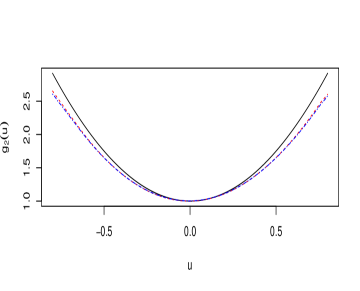
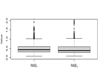
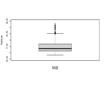
($\rm{\@slowromancap ii@}$) In Figures 1-2, the performances of estimator $\hat{{g}_{1}}(\cdot)$ and $\hat{{g}_{2}}(\cdot)$ will be exhibited by using the square root of average square errors (RASE):

$$\mathrm{RASE}_{k}=\left\{N^{-1}\sum_{j=1}^{N}[\hat{g}_{k}(u_{j})-g_{k}(u_{j})]^{2}\right\}^{1/2},\quad k=1,2,$$

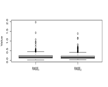
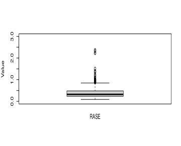
where $\{u_{j},j=1,\ldots,N\}$ are the regular grid points at which the function $\hat{{g}_{k}}(u)$ is evaluated. In our simulation, $N=20$ is used. The performance of estimator $\hat{\bm{g}}(\cdot)$ will be assessed by $\rm{RASE}=\rm{RASE_{1}}+\rm{RASE_{2}}$.

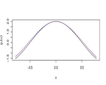
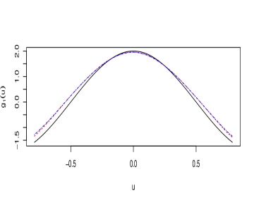
From Figures 1-2, we can see that the estimated coefficient function curves of $g_{1}(u)$ and $g_{2}(u)$ by SCAD and LASSO are both close to the true coefficient function curves. As the level of model errors decreases, the estimated curves become slightly close to the true curves.

Table 1: Simulation results for the estimator of $\beta$ and $\theta$($\varepsilon_{i}\sim N(0,0.5^{2}))$

		Estimator of $\beta$					Estimator of $\theta$
$n$	Method	Mean	Bias	SD	C	I	GMSE	C	I
100	SCAD	0.99522	-0.00478	0.02335	6.45200	0.00400	0.00938	6.71400	0
	LASSO	0.99578	-0.00422	0.02151	6.38200	0.00400	0.01111	6.66800	0
	Oracle	0.99636	-0.00401	0.01987	7	0	0.00899	7	0
150	SCAD	0.99826	-0.00174	0.00263	6.63800	0.00200	0.00527	6.85400	0
	LASSO	0.99822	-0.00178	0.00232	6.54800	0	0.00633	6.80600	0
	Oracle	0.99835	-0.00170	0.00224	7	0	0.00512	7	0
200	SCAD	0.99950	-0.00050	0.00025	6.98600	0	0.00390	6.99000	0
	LASSO	0.99949	-0.00051	0.00025	6.95000	0	0.00476	6.96600	0
	Oracle	0.99958	-0.00049	0.00023	7	0	0.00387	7	0

Table 2: Simulation results for the estimator of $\beta$ and $\theta$($\varepsilon_{i}\sim N(0,1.5^{2}))$

		Estimator of $\beta$					Estimator of $\theta$
$n$	Method	Mean	Bias	SD	C	I	GMSE	C	I
100	SCAD	0.97324	-0.02676	0.07658	6.22300	0	0.08017	6.18200	0
	LASSO	0.97176	-0.02824	0.08754	6.20000	0	0.08279	6.11600	0
	Oracle	0.97412	-0.02567	0.06387	7	0	0.07377	7	0
150	SCAD	0.98886	-0.01114	0.01956	6.45100	0	0.04531	6.48600	0
	LASSO	0.98836	-0.01164	0.02056	6.44600	0	0.04775	6.44400	0
	Oracle	0.98987	-0.01022	0.01814	7	0	0.04456	7	0
200	SCAD	0.99848	-0.00152	0.00347	6.81200	0	0.03876	6.62600	0
	LASSO	0.99850	-0.00149	0.00339	6.80000	0	0.03913	6.59800	0
	Oracle	0.99911	-0.00146	0.00325	7	0	0.03747	7	0

Figure 1: Simulation results when the $\varepsilon_{i}$ is independent $N(0,0.5^{2})$ and $n=100$. The left panel shows the true curve(black solid curve), the SCAD estimated curve(red dashed curve) and the LASSO estimated curve(blue longdash curve) of $g_{1}(u)$. The right panel shows the true curve(black solid curve), the SCAD estimated curve(red dashed curve) and the LASSO estimated curve(blue longdash curve) of $g_{2}(u)$.

Figure 2: Simulation results when the $\varepsilon_{i}$ is independent $N(0,0.5^{2})$ and $n=100$. The left panel is the boxplot the 500 $\rm{RASE_{1}}$ and $\rm{RASE_{2}}$ values of $g_{1}(u)$ and $g_{2}(u)$. The right panel is the boxplot the 500 RASE values of $\bm{g}(u)$.

Figure 3: Simulation results when the $\varepsilon_{i}$ is independent $N(0,1.5^{2})$ and $n=100$. The left panel shows the true curve(black solid curve), the SCAD estimated curve(red dashed curve) and the LASSO estimated curve(blue longdash curve) of $g_{1}(u)$. The right panel shows the true curve(black solid curve), the SCAD estimated curve(red dashed curve) and the LASSO estimated curve(blue longdash curve) of $g_{2}(u)$.

Figure 4: Simulation results when the $\varepsilon_{i}$ is independent $N(0,1.5^{2})$ and $n=100$. The left panel is the boxplot the 500 $\rm{RASE_{1}}$ and $\rm{RASE_{2}}$ values of $g_{1}(u)$ and $g_{2}(u)$. The right panel is the boxplot the 500 RASE values of $\bm{g}(u)$.

4.2 Application to the body fat dataset

We illustrate our proposed variable selection method by applying the body fat dataset, which is available from the website (http://lib.stat.cmu.edu/datasets/bodyfat). The response variable is the percentage of body fat which is determined by the underwater weighting technique (Siri, (1956) [32]). The thirteen covariates in this dataset are Age, Weight, Height, Neck, Chest, Abdomen, Hip, Thigh, Knee, Ankle, Biceps, Forearm and Wrist. The entire dateset contains 252 observations. Two observations are apparently type errors, four observations show inconsistency between the percentage of body fat and body density. These six observations can be removed from the dataset as outliers. In the following analysis, we employ the remain 246 observations.

In order to fit our model, we take logarithm of the percentage of body fat as the response variable $Y$, the covariates for linear part $U_{1}$=Age, $U_{2}$=Weight, the covariates dependent on varying coefficients $Z_{1}$=1, $Z_{2}$=Height, the index covariates $X_{1}$=Neck, $X_{2}$=Chest, $X_{3}$=Abdomen, $X_{4}$=Hip, $X_{5}$=Thigh, $X_{6}$=Knee, $X_{7}$=Ankle, $X_{8}$=Biceps, $X_{9}$=Forearm and $X_{10}$=Wrist. Then, we will establish the partially linear single-index variable-coefficient model (PLSIVM) as follows:

$$Y=\theta_{1}U_{1}+\theta_{2}U_{2}+{g}(\beta^{T}X)Z_{1}+{g}(\beta^{T}X)Z_{2}+\varepsilon,$$

where $\beta^{T}X=\beta_{1}X_{1}+\cdots+\beta_{10}X_{10}$. For the PLSIVM, the restriction $\|\beta\|=1$ is required for identifiability.

From Table 3, we can obtain that:

(1) The proposed variable selection method chooses five covariates: Age($U_{1}$), Weight
($U_{2}$), Neck($X_{1}$), Abdomen($X_{3}$), Wrist($X_{10}$). Among these significant covariates, Abdomen is the most important measurement for the prediction of the percentage of body fat, Wrist has more significant effects than Age, Weight and Neck, which is coincident with the results in Peng and Huang (2011) [29] and Lin and Huang (2013) [23].

(2) It is worth noting that Weight has nonzero constant on $Y$ which is similar to LM while is different from the existed results of SIM in Peng and Huang (2011) [29], STM in Lin and Huang (2013) [23] and SIVCM in Feng and Xue (2015) [9].

(3) The multiple $R^{2}$=0.70158 which is slightly larger than that of other four models. Therefore, our proposed variable selection method for PLSIVM is more appropriate to fit the body fat dataset.

Table 3: Estimation results of body fat data

Method	PLSIVCM	SIVCM	SIM	STM	LM
Age	0.00575	0.00820	0.01490	0.08330	0.04890
Weight	0.00595	0	0	0	0.14570
Height	0	0	0	-0.10140	-0.03950
Neck	-0.09926	-0.09900	-0.16910	-0.02800	-0.14080
Chest	0	0	0	0	-0.09430
Abdomen	0.96980	0.96910	0.96060	0.97670	0.76630
Hip	0	0	0	0	-0.36380
Thigh	0	0	0	0	0.14610
Knee	0	0	0	0	0
Ankle	0	0	0	0	0
Biceps	0	0	0	0	0
Forearm	0	0	0	0	0.04130
Wrist	-0.14629	-0.22600	-0.22020	-0.16770	-0.11860
$R^{2}$	0.70158	0.68160	0.67380	0.66650	0.61480

Appendix. Proof of theorems

We begin the Appendix by listing some regularity conditions that are used in this paper. For convenience and simplicity, let $C$ denote a positive constant that may be different at each appearance throughout this paper.

(C1) The density function $f(u)$ of $\beta_{0}^{\mathrm{T}}X,$ is bounded away from 0 on $\mathscr{U}=$ $\{u=\beta^{\mathrm{T}}x\colon x\in A\}$, where $A$ is the bounded support set of $X$. Furthermore, we assume that $f(u)$ satisfies the Lipschitz condition of order 1 on $\mathscr{U}.$

(C2) The function $g_{j}(u)$, $j=1,\ldots,q$, have bounded and continuous derivatives up to order $r(\geqslant 2)$ on $\mathscr{U}$, where $g_{j}(u)$ is the $j$th component of $\bm{g}(u).$

(C3) $E(\|X\|^{6})<\infty$, $E(\|U\|^{6})<\infty$, $E(\|Z\|^{6})<\infty$, and $E(|\varepsilon|^{6})<\infty.$

(C4) Let $c_{1},\ldots,c_{K}$ be the interior knots of $[a,b]$, where $a=\inf\{u\colon u\in\mathscr{U}\},\quad b=\sup\{u\colon u\in\mathscr{U}\}.$ Furthermore, we let $c_{0}=a,\quad c_{K+1}=b,\quad h_{i}=c_{i}-c_{i-1},\quad h=\max\{h_{i}\}.$ Then, there exists a constant $C_{0}$ such that

$$\frac{h}{\min\{h_{i}\}}<C_{0},\quad\max\{h_{i+1}-h_{i}\}=o(K^{-1}).$$

(C5) $b_{n}\to 0$, as $n\to\infty$, where

$$b_{n}=\operatorname*{max}_{l,h,k}\left\{|\ddot{p}_{\lambda_{1l}}(|\phi_{l0}|)|,\>|\ddot{p}_{\lambda_{2h}}(|\theta_{h0}|),|\ddot{p}_{\lambda_{3k}}(\|\gamma_{k0}\|_{H})|\colon\phi_{l0}\neq 0,\theta_{h0}\neq 0,\>\gamma_{k0}\neq 0\right\}.$$

(C6) The penalty functions satisfy

$$\mathop{\lim\inf}_{n\to\infty}\mathop{\lim\inf}_{\phi_{l}\to 0^{+}}\lambda_{1l}^{-1}|\dot{p}_{\lambda_{1l}}(|\phi_{l}|)|>0,\quad\mathop{\lim\inf}_{n\to\infty}\mathop{\lim\inf}_{\theta_{h}\to 0^{+}}\lambda_{2h}^{-1}|\dot{p}_{\lambda_{2h}}(|\theta_{h}|)|>0,$$

$$\mathop{\lim\inf}_{n\to\infty}\mathop{\lim\inf}_{\|\gamma_{k}\|_{H}\to 0}\lambda_{3k}^{-1}|\dot{p}_{\lambda_{3k}}(\|\gamma_{k}\|_{H})|>0,$$

where $l=s,\ldots,p-1$, $h=w+1,\ldots,d$, $k=v+1,\ldots,q.$

(C7) The matrix $D(u)=E\{Z^{*}Z^{*\text{T}}\mid\beta_{0}^{*\text{T}}X^{*}=u\}$ is positive definite, and each element of $D(u)$, $C_{1}(u)=E\{V^{*}Z^{*\mathrm{T}}\mid\beta_{0}^{*\mathrm{T}}X^{*}=u\}$ and $C_{2}(u)=E\{U^{*}Z^{*\mathrm{T}}\mid\beta_{0}^{*\mathrm{T}}X^{*}=u\}$ satisfies the Lipschitz condition of order 1 on $\mathscr{U}$, where

$$V^{*}=\dot{\bm{g}}_{0}^{\mathrm{T}}(\beta_{0}^{\mathrm{*T}}X^{*})Z^{*}J_{\phi_{0}^{*}}^{\mathrm{T}}X^{*}.$$

Remark 2.

Condition (C1) is used to bound the density function $f(u)$ of $\beta_{0}^{\mathrm{T}}X$ away from 0. Condition (C2) is the standard smoothness and continuity condition in the nonparametric estimation procedure. Condition (C3) is the necessary condition for the asymptotic properties of the estimators. Condition (C4) indicates that $c_{0},\ldots,c_{K+1}$ is a $C_{0}$-quasi-uniform sequence of partitions of [0,1]. Condition (C5) and Condition (C6) are assumptions on the penalty functions. Condition (C7) ensures that the limiting variance for the estimator of $\beta_{0}$ and $\theta_{0}$ exists.

To obtain the proofs of the theorems, the following lemmas are required.

Lemma 1.

If $g_{k}(u)$, $k=1,\ldots,q$, satisfy condition (C2), then there exists $a$ constant $C>0$ depending only on $M$ such that

$$\sup\limits_{u\in\mathscr{U}}|g_{k}(u)-B^{\mathrm{T}}(u)\gamma_{k}|\leqslant CK^{-r}.$$

$\mathbf{Proof}$ This result is due to Corollary 6.21 in Schumaker (1981) [31], we omit the details here.$\hfill\square$

Lemma 2.

Suppose that conditions (C1)-(C3) and (C7) hold, and the number of knots $K=O(n^{-r/(2r+1)}).$ Then we have

$$\dfrac{1}{n}\sum_{i=1}^{n}V_{i}^{*}V_{i}^{*\text{T}}-\Psi_{n}^{\text{T}}\Phi_{n}^{-1}\Psi_{n}\xrightarrow{P}\Sigma_{11},\quad\dfrac{1}{n}\sum_{i=1}^{n}V_{i}^{*}U_{i}^{*\text{T}}-\Psi_{n}^{\text{T}}\Phi_{n}^{-1}G_{n}\xrightarrow{P}\Sigma_{12},$$

$$\dfrac{1}{n}\sum_{i=1}^{n}U_{i}^{*}V_{i}^{*\text{T}}-G_{n}^{\text{T}}\Phi_{n}^{-1}\Psi_{n}\xrightarrow{P}\Sigma_{21},\quad\dfrac{1}{n}\sum_{i=1}^{n}U_{i}^{*}U_{i}^{*\text{T}}-G_{n}^{\text{T}}\Phi_{n}^{-1}G_{n}\xrightarrow{P}\Sigma_{22},$$

and

$$\begin{pmatrix}\frac{1}{n}\sum_{i=1}^{n}V_{i}^{*}V_{i}^{*\mathrm{T}}-\Psi_{n}^{\mathrm{T}}\Phi_{n}^{-1}\Psi_{n}&\frac{1}{n}\sum_{i=1}^{n}V_{i}^{*}U_{i}^{*\mathrm{T}}-\Psi_{n}^{\mathrm{T}}\Phi_{n}^{-1}G_{n}\\ \frac{1}{n}\sum_{i=1}^{n}U_{i}^{*}V_{i}^{*\mathrm{T}}-G_{n}^{\mathrm{T}}\Phi_{n}^{-1}\Psi_{n}&\frac{1}{n}\sum_{i=1}^{n}U_{i}^{*}U_{i}^{*\mathrm{T}}-G_{n}^{\mathrm{T}}\Phi_{n}^{-1}G_{n}\end{pmatrix}\xrightarrow{P}\Sigma,$$

where ${\Sigma=\begin{pmatrix}\Sigma_{11}&\Sigma_{12}\\ \Sigma_{21}&\Sigma_{22}\end{pmatrix},}$ $\Phi_{n}=\frac{1}{n}\sum_{i=1}^{n}W_{i}^{*}(\phi_{0}^{*})W_{i}^{*\mathrm{T}}(\phi_{0}^{*})$, $\Psi_{n}=\frac{1}{n}\sum_{i=1}^{n}W_{i}^{*}(\phi_{0}^{*})V_{i}^{*\mathrm{T}}$, $G_{n}=\frac{1}{n}\sum_{i=1}^{n}W_{i}^{*}(\phi_{0}^{*})U_{i}^{*\mathrm{T}}$, and ‘$\xrightarrow{P}$’ means the convergence in probability.

$\mathbf{Proof}$ Let $\mathbf{W}^{*}=(W_{1}^{*}(\phi_{0}^{*}),\ldots,W_{n}^{*}(\phi_{0}^{*}))^{\mathrm{T}}$, $\mathbf{V}^{*}=(V_{1}^{*},\ldots,V_{n}^{*})^{\mathrm{T}}$, $\mathbf{U}^{*}=(U_{1}^{*},\ldots,U_{n}^{*})^{\mathrm{T}}$, $\mathbf{V}^{*}=\mathbf{V}^{*}-\Gamma_{n}+\Gamma_{n}=:\Delta_{n}+\Gamma_{n}$, $\mathbf{U}^{*}=\mathbf{U}^{*}-\Omega_{n}+\Omega_{n}=:\Xi_{n}+\Omega_{n},$ where

$$V_{i}^{*}=\dot{\bm{g}}^{\mathrm{T}}(\beta_{0}^{*\mathrm{T}}X_{i}^{*})Z_{i}^{*}J_{\phi_{0}^{*}}^{\mathrm{T}}X_{i}^{*},\quad W_{i}^{*}(\phi_{0}^{*})=I_{q}\otimes B(\beta_{0}^{*\mathrm{T}}X_{i}^{*})Z_{i}^{*},$$

$$\Gamma_{n}=(C_{1}(\beta_{0}^{*\mathrm{T}}X_{1}^{*})D^{-1}(\beta_{0}^{*\mathrm{T}}X_{1}^{*})Z_{1}^{*},\ldots,C_{1}(\beta_{0}^{*\mathrm{T}}X_{n}^{*})D^{-1}(\beta_{0}^{*\mathrm{T}}X_{n}^{*})Z_{n}^{*})^{\mathrm{T}},$$

$$\Omega_{n}=(C_{2}(\beta_{0}^{*\mathrm{T}}X_{1}^{*})D^{-1}(\beta_{0}^{*\mathrm{T}}X_{1}^{*})Z_{1}^{*},\ldots,C_{2}(\beta_{0}^{*\mathrm{T}}X_{n}^{*})D^{-1}(\beta_{0}^{*\mathrm{T}}X_{n}^{*})Z_{n}^{*})^{\mathrm{T}}.$$

Then a simple calculation yields

$$\frac{1}{n}\sum_{i=1}^{n}V_{i}^{*}V_{i}^{*\mathrm{T}}-\Psi_{n}^{\mathrm{T}}\Phi_{n}^{-1}\Psi_{n}$$

$$=~ n^{-1}\mathbf{V}^{*\mathrm{T}}(I-P^{\mathrm{T}})(I-P)\mathbf{V}^{*}$$

$$=~ n^{-1}(\Delta_{n}+\Gamma_{n})^{\mathrm{T}}(I-P^{\mathrm{T}})(I-P)(\Delta_{n}+\Gamma_{n})$$

$$=~ n^{-1}\{\Delta_{n}^{\mathrm{T}}\Delta_{n}+\Delta_{n}^{\mathrm{T}}(I-P^{\mathrm{T}})(I-P)\Gamma_{n}+\Gamma_{n}^{\mathrm{T}}(I-P^{\mathrm{T}})(I-P)\Delta_{n}$$

$$+\Gamma_{n}^{\mathrm{T}}(I-P^{\mathrm{T}})(I-P)\Gamma_{n}-\Delta_{n}^{\mathrm{T}}P^{\mathrm{T}}P\Delta_{n}\},$$ (4.1)

$$\frac{1}{n}\sum_{i=1}^{n}V_{i}^{*}U_{i}^{*\mathrm{T}}-\Psi_{n}^{\mathrm{T}}\Phi_{n}^{-1}G_{n}$$

$$=~ n^{-1}\mathbf{V}^{*\mathrm{T}}(I-P^{\mathrm{T}})(I-P)\mathbf{U}^{*}$$

$$=~ n^{-1}(\Delta_{n}+\Gamma_{n})^{\mathrm{T}}(I-P^{\mathrm{T}})(I-P)(\Xi_{n}+\Omega_{n})$$

$$=~ n^{-1}\{\Delta_{n}^{\mathrm{T}}\Xi_{n}+\Delta_{n}^{\mathrm{T}}(I-P^{\mathrm{T}})(I-P)\Omega_{n}+\Gamma_{n}^{\mathrm{T}}(I-P^{\mathrm{T}})(I-P)\Xi_{n}$$

$$+\Gamma_{n}^{\mathrm{T}}(I-P^{\mathrm{T}})(I-P)\Omega_{n}-\Delta_{n}^{\mathrm{T}}P^{\mathrm{T}}P\Xi_{n}\},$$ (4.2)

$$\frac{1}{n}\sum_{i=1}^{n}U_{i}^{*}V_{i}^{*\mathrm{T}}-G_{n}^{\mathrm{T}}\Phi_{n}^{-1}\Psi_{n}$$

$$=~ n^{-1}\mathbf{U}^{*\mathrm{T}}(I-P^{\mathrm{T}})(I-P)\mathbf{V}^{*}$$

$$=~ n^{-1}(\Xi_{n}+\Omega_{n})^{\mathrm{T}}(I-P^{\mathrm{T}})(I-P)(\Delta_{n}+\Gamma_{n})$$

$$=~ n^{-1}\{\Xi_{n}^{\mathrm{T}}\Delta_{n}+\Xi_{n}^{\mathrm{T}}(I-P^{\mathrm{T}})(I-P)\Gamma_{n}+\Omega_{n}^{\mathrm{T}}(I-P^{\mathrm{T}})(I-P)\Delta_{n}$$

$$+\Omega_{n}^{\mathrm{T}}(I-P^{\mathrm{T}})(I-P)\Gamma_{n}-\Xi_{n}^{\mathrm{T}}P^{\mathrm{T}}P\Delta_{n}\},$$ (4.3)

and

$$\frac{1}{n}\sum_{i=1}^{n}U_{i}^{*}U_{i}^{*\mathrm{T}}-G_{n}^{\mathrm{T}}\Phi_{n}^{-1}G_{n}$$

$$=~ n^{-1}\mathbf{U}^{*\mathrm{T}}(I-P^{\mathrm{T}})(I-P)\mathbf{U}^{*}$$

$$=~ n^{-1}(\Xi_{n}+\Omega_{n})^{\mathrm{T}}(I-P^{\mathrm{T}})(I-P)(\Xi_{n}+\Omega_{n})$$

$$=~ n^{-1}\{\Xi_{n}^{\mathrm{T}}\Xi_{n}+\Xi_{n}^{\mathrm{T}}(I-P^{\mathrm{T}})(I-P)\Omega_{n}+\Omega_{n}^{\mathrm{T}}(I-P^{\mathrm{T}})(I-P)\Xi_{n}$$

$$+\Omega_{n}^{\mathrm{T}}(I-P^{\mathrm{T}})(I-P)\Omega_{n}-\Xi_{n}^{\mathrm{T}}P^{\mathrm{T}}P\Xi_{n}\},$$ (4.4)

where $P=\mathbf{W}^{*}(\mathbf{W}^{*\mathrm{T}}\mathbf{W}^{*})^{-1}\mathbf{W}^{*\mathrm{T}}.$

By the proof of Lemma 1 in Zhao and Xue (2010) [53], we easily obtain that all but the first term of (4.1), (4.2), (4.3) and (4.4) are $o_{p}(1)$. Then, by the law of large numbers, we can derive that the first term converges to $\Sigma_{11}$, $\Sigma_{12}$, $\Sigma_{21}$ and $\Sigma_{22}$ respectively. Hence, we have

$$\begin{pmatrix}\frac{1}{n}\sum_{i=1}^{n}V_{i}^{*}V_{i}^{*\mathrm{T}}-\Psi_{n}^{\mathrm{T}}\Phi_{n}^{-1}\Psi_{n}&\frac{1}{n}\sum_{i=1}^{n}V_{i}^{*}U_{i}^{*\mathrm{T}}-\Psi_{n}^{\mathrm{T}}\Phi_{n}^{-1}G_{n}\\ \frac{1}{n}\sum_{i=1}^{n}U_{i}^{*}V_{i}^{*\mathrm{T}}-G_{n}^{\mathrm{T}}\Phi_{n}^{-1}\Psi_{n}&\frac{1}{n}\sum_{i=1}^{n}U_{i}^{*}U_{i}^{*\mathrm{T}}-G_{n}^{\mathrm{T}}\Phi_{n}^{-1}G_{n}\end{pmatrix}\xrightarrow{P}\Sigma.$$

$\hfill\square$
$\mathbf{Proof~of~Theorem~1}$ Let $\delta=n^{-r/(2r+1)}+a_{n}$, $\phi=\phi_{0}+\delta\tau_{1}$, $\theta=\theta_{0}+\delta\tau_{2}$, $\gamma=\gamma_{0}+\delta\tau_{3}$,  $\tau=(\tau_{1}^{\mathrm{T}}$,$\tau_{2}^{\mathrm{T}}$,$\tau_{3}^{\mathrm{T}})^{\mathrm{T}}.$

(i) We will show that, for any given $\epsilon>0$, there exists a large constant $C$ such that

$$P\Big{\{}\inf\limits_{\|\tau\|=C}Q(\phi,\theta,\gamma)>Q(\phi_{0},\theta_{0},\gamma_{0})\Big{\}}\geqslant 1-\epsilon,$$ (4.5)

where $\phi_{0}$, $\theta_{0}$ and $\gamma_{0}$ are true value of $\phi$, $\theta$ and $\gamma$.

Let $L_{n}(\tau)=K^{-1}\{Q(\phi,\theta,\gamma)-Q(\phi_{0},\theta_{0},\gamma_{0})\}.$ Thus, by the Taylor expansion and a direct calculation, we have

$$L_{n}(\tau)=~ K^{-1}\{Q(\phi_{0}+\delta\tau_{1},\theta_{0}+\delta\tau_{2},\gamma_{0}+\delta\tau_{3})-Q(\phi_{0},\theta_{0},\gamma_{0})\}$$

$$\geqslant~ \frac{-2\delta}{K}\sum_{i=1}^{n}(Y_{i}-\theta_{0}^{\mathrm{T}}U_{i}-W_{i}(\phi_{0})^{\mathrm{T}}\gamma_{0})(\dot{W}_{i}^{\mathrm{T}}(\phi_{0})\gamma_{0}\tau_{1}^{\mathrm{T}}J_{\phi_{0}}^{\mathrm{T}}X_{i}+U^{\mathrm{T}}\tau_{2}+W_{i}^{\mathrm{T}}(\phi_{0})\tau_{3})$$

$$+\frac{\delta^{2}}{K}\sum_{i=1}^{n}(\dot{W}_{i}^{\mathrm{T}}(\phi_{0})\gamma_{0}\tau_{1}^{\mathrm{T}}J_{\phi_{0}}^{\mathrm{T}}X_{i}+U^{\mathrm{T}}\tau_{2}+W_{i}^{\mathrm{T}}(\phi_{0})\tau_{3})^{2}$$

$$+\frac{n}{K}\sum_{l=1}^{s-1}[p_{\lambda_{1l}}(|\phi_{l}|)-p_{\lambda_{1l}}(|\phi_{l0}|)]$$

$$+\frac{n}{K}\sum_{h=1}^{w}[p_{\lambda_{2h}}(|\theta_{h}|)-p_{\lambda_{2h}}(|\theta_{h0}|)]$$

$$+\frac{n}{K}\sum_{k=1}^{v}[p_{\lambda_{3k}}(\|\gamma_{k}\|_{H})-p_{\lambda_{3k}}(\|\gamma_{k0}\|_{H})]+o_{p}(1),$$

Let $\dot{W}_{i}(\phi_{0})=I_{q}\otimes\dot{B}(\beta_{0}^{\mathrm{T}}X_{i})Z_{i},$ $R(u)=\left(R_{1}(u),\ldots,R_{q}(u)\right)^{\mathrm{T}}$, $R_{k}(u)=g_{k0}(u)-B^{\mathrm{T}}(u)\gamma_{k0},$ $k=1,\ldots,q.$ Since $Y_{i}=\theta_{0}^{T}U_{i}+\bm{g}_{0}^{T}(\beta_{0}^{T}X_{i})Z_{i}+\varepsilon_{i}$, we can obtain that

$$Y_{i}-\theta_{0}^{\mathrm{T}}U_{i}-W_{i}(\phi_{0})^{\mathrm{T}}\gamma_{0}$$

$$= \theta_{0}^{T}U_{i}+\bm{g}_{0}^{T}(\beta_{0}^{T}X_{i})Z_{i}+\varepsilon_{i}-\theta_{0}^{\mathrm{T}}U_{i}-W_{i}(\phi_{0})^{\mathrm{T}}\gamma_{0}$$

$$= \varepsilon_{i}+\bm{g}_{0}^{T}(\beta_{0}^{T}X_{i})Z_{i}-W_{i}(\phi_{0})^{\mathrm{T}}\gamma_{0}$$

$$= \varepsilon_{i}+R^{\mathrm{T}}(\beta_{0}^{\mathrm{T}}X_{i})Z_{i}.$$

Then we can write

$$L_{n}(\tau)\geqslant~ \frac{-2\delta}{K}\sum_{i=1}^{n}(\varepsilon_{i}+R^{\mathrm{T}}(\beta_{0}^{\mathrm{T}}X_{i})Z_{i})(\dot{W}_{i}^{\mathrm{T}}(\phi_{0})\gamma_{0}\tau_{1}^{\mathrm{T}}J_{\phi_{0}}^{\mathrm{T}}X_{i}+U^{\mathrm{T}}\tau_{2}+W_{i}^{\mathrm{T}}(\phi_{0})\tau_{3})$$

$$+\frac{\delta^{2}}{K}\sum_{i=1}^{n}(\dot{W}_{i}^{\mathrm{T}}(\phi_{0})\gamma_{0}\tau_{1}^{\mathrm{T}}J_{\phi_{0}}^{\mathrm{T}}X_{i}+U^{\mathrm{T}}\tau_{2}+W_{i}^{\mathrm{T}}(\phi_{0})\tau_{3})^{2}+o_{p}(1)$$

$$+\frac{n}{K}\sum_{l=1}^{s-1}[p_{\lambda_{1l}}(|\phi_{l}|)-p_{\lambda_{1l}}(|\phi_{l0}|)]$$

$$+\frac{n}{K}\sum_{h=1}^{w}[p_{\lambda_{2h}}(|\theta_{h}|)-p_{\lambda_{2h}}(|\theta_{h0}|)]$$

$$+\frac{n}{K}\sum_{k=1}^{v}[p_{\lambda_{3k}}(\|\gamma_{k}\|_{H})-p_{\lambda_{3k}}(\|\gamma_{k0}\|_{H})],$$

$$=:~ S_{1}+S_{2}+S_{3}+S_{4}+S_{5}+o_{p}(1).$$ (4.6)

Next, we analyse each term of (4.6). For $S_{1}$, by conditions (C1), (C2), (C4), and Lemma 1, we can derive that

$$\|R_{k}(u)\|=O(K^{-r})$$

and

$$|\dot{g}_{k}(\beta_{0}^{\mathrm{T}}X_{i})-\dot{B}^{\mathrm{T}}(\beta_{0}^{\mathrm{T}}X_{i})\gamma_{k0}|\leqslant CK^{-r+1}.$$ (4.7)

Then, a simple calculation yields

$$\sum_{i=1}^{n}R^{\mathrm{T}}(\beta_{0}^{\mathrm{T}}X_{i})Z_{i}\{\dot{W}_{i}^{\mathrm{T}}(\phi_{0})\gamma_{0}\tau_{1}^{\mathrm{T}}J_{\phi_{0}}^{\mathrm{T}}X_{i}+U^{\mathrm{T}}\tau_{2}+W_{i}^{\mathrm{T}}(\phi_{0})\tau_{3}\}$$

$$=~ \sum_{i=1}^{n}R^{\mathrm{T}}(\beta_{0}^{\mathrm{T}}X_{i})Z_{i}\{\dot{\bm{g}}^{\mathrm{T}}(\beta_{0}^{\mathrm{T}}X_{i})Z_{i}\tau_{1}^{\mathrm{T}}J_{\phi_{0}}^{\mathrm{T}}X_{i}$$

$$+(\dot{W}_{i}^{\mathrm{T}}(\phi_{0})\gamma_{0}-\dot{\bm{g}}^{\mathrm{T}}(\beta_{0}^{\mathrm{T}}X_{i})Z_{i})\tau_{1}^{\mathrm{T}}J_{\phi_{0}}^{\mathrm{T}}X_{i}+U^{\mathrm{T}}\tau_{2}+W_{i}^{\mathrm{T}}(\phi_{0})\tau_{3}\}$$

$$=~ O_{p}(nK^{-r}\|\tau\|).$$ (4.8)

Note that $\varepsilon_{i}$ is independent of $(X_{i},U_{i},Z_{i})$. We can prove that

$$\frac{1}{\sqrt{n}}\sum_{i=1}^{n}\varepsilon_{i}\{\dot{W}_{i}^{\mathrm{T}}(\phi_{0})\gamma_{0}\tau_{1}^{\mathrm{T}}J_{\phi_{0}}^{\mathrm{T}}X_{i}+U^{\mathrm{T}}\tau_{2}+W_{i}^{\mathrm{T}}(\phi_{0})\tau_{3}\}=O_{p}(\|\tau\|).$$

Combing this with (4.8), we can get that

$$S_{1}=O_{p}(\sqrt{n}\>K^{-1}\delta)\|\tau\|+O_{p}(nK^{-1-r}\delta)\|\tau\|=O_{p}(1+n^{r/(2r+1)}a_{n})\|\tau\|.$$

Similarly, we can prove that

$$S_{2}=O_{p}(nK^{-1}\delta^{2})\|\tau\|^{2}=O_{p}(1+2n^{r/(2r+1)}a_{n})\|\tau\|^{2}.$$

Hence, by choosing a sufficiently large $C$, $S_{2}$ dominates $S_{1}$ uniformly in $\|\tau\|=C.$

By the fact that $p_{\lambda}(0)=0$ and the Taylor expansion, we get

$$S_{3} \leqslant\frac{n}{K}\sum_{l=1}^{s-1}[\delta\dot{p}_{\lambda_{1l}}(|\phi_{l0}|)\mathrm{sgn}(\phi_{l0})|\tau_{1l}|+\delta^{2}\ddot{p}_{\lambda_{1l}}(|\phi_{l0}|)|\tau_{1l}|^{2}\{1+o(1)\}]$$

$$\leqslant\sqrt{s-1}\>K^{-1}n\delta a_{n}\|\tau\|+nK^{-1}\delta^{2}b_{n}\|\tau\|^{2},$$

$$S_{4} \leqslant\frac{n}{K}\sum_{l=1}^{w}[\delta\dot{p}_{\lambda_{2h}}(|\theta_{h0}|)\mathrm{sgn}(\theta_{h0})|\tau_{2h}|+\delta^{2}\ddot{p}_{\lambda_{2h}}(|\theta_{h0}|)|\tau_{2h}|^{2}\{1+o(1)\}]$$

$$\leqslant\sqrt{w}\>K^{-1}n\delta a_{n}\|\tau\|+nK^{-1}\delta^{2}b_{n}\|\tau\|^{2},$$

$$S_{5} \leqslant\frac{n}{K}\sum_{l=1}^{v}[\delta\dot{p}_{\lambda_{3k}}(|\gamma_{k0}|)\mathrm{sgn}(\gamma_{k0})|\tau_{3k}|+\delta^{2}\ddot{p}_{\lambda_{3k}}(|\gamma_{k0}|)|\tau_{3k}|^{2}\{1+o(1)\}]$$

$$\leqslant\sqrt{v}\>K^{-1}n\delta a_{n}\|\tau\|+nK^{-1}\delta^{2}b_{n}\|\tau\|^{2}.$$

Then, it is easy to show that $S_{3}$, $S_{4}$ and $S_{5}$ are dominated by $S_{2}$ uniformly in $\|\tau\|=C.$ Hence, for a sufficiently large $C$, the probability of $L_{n}(\tau)=K^{-1}\{Q(\phi,\theta,\gamma)-Q(\phi_{0},\theta_{0},\gamma_{0})\}>0$ is at least $1-\epsilon$, then, we can reach to (4.5). Therefore, there exist local minimizers $\hat{\phi}$, $\hat{\theta}$ and $\hat{\gamma}$ such that

$$\|\hat{\phi}-\phi_{0}\|=O_{p}(\delta),\quad\|\hat{\theta}-\theta_{0}\|=O_{p}(\delta),\quad\|\hat{\gamma}-\gamma_{0}\|=O_{p}(\delta).$$

$\begin{array}[]{l}\text{A direct calculation can lead to }\|\hat{\beta}-\beta_{0}\|=O_{p}(\delta),\mathrm{~which~completes~the~proofs}\\ \text{of (i).}\end{array}$

(ii) It can be proved directly from the proof of (i).

(iii) Note that

$$\|\hat{g}_{k}(u)-g_{k0}(u)\|^{2} =\>\int_{\mathscr{U}}\{\hat{g}_{k}(u)-g_{k0}(u)\}^{2}\mathrm{d}u$$

$$=\>\int_{\mathscr{U}}\{B^{\mathrm{T}}(u)\hat{\gamma}_{k}-B^{\mathrm{T}}(u)\gamma_{k0}-R_{k}(u)\}^{2}\mathrm{d}u$$

$$\leqslant 2\int_{\mathscr{U}}\{B^{\mathrm{T}}(u)\hat{\gamma}_{k}-B^{\mathrm{T}}(u)\gamma_{k0}\}^{2}\mathrm{d}u+2\int_{\mathscr{U}}R_{k}^{2}(u)\mathrm{d}u$$

$$=2(\hat{\gamma}_{k}-\gamma_{k0})^{\mathrm{T}}H(\hat{\gamma}_{k}-\gamma_{k0})+2\int_{\mathscr{U}}R_{k}(u)^{2}\mathrm{d}u.$$

This, together with $\|H\|=O(1)$, can lead to

$$(\hat{\gamma}_{k}-\gamma_{k0})^{\mathrm{T}}H(\hat{\gamma}_{k}-\gamma_{k0})=O_{p}(n^{-2r/(2r+1)}+a_{n}^{2}).$$ (4.9)

In addition, it is easy to show that

$$\int_{\mathcal{U}}R_{k}^{2}(u)\mathrm{d}u=O_{p}(n^{-2r/(2r+1)}).$$ (4.10)

By using (4.9) and (4.10), we complete the proof of (iii).$\hfill\square$

$\mathbf{Proof~of~Theorem~2}$ (i) By $\lambda_{\max}\to$0, it is easy to show that $a_{n}=0$ for large $n.$ Then by Theorem 1, it is sufficient to show that, for any $\phi_{j}$,

$$\|\phi_{j}-\phi_{j0}\|=O_{p}(n^{-r/(2r+1)}),\quad j=1,\ldots,s-1,$$

and given small $\epsilon=Cn^{-r/(2r+1)}$, when $n\to\infty$, with probability approaching to one, it holds that

$$\frac{\partial Q(\phi,\theta,\gamma)}{\partial\phi_{j}}>0,\quad 0<\phi_{j}<\epsilon,\quad j=s,\ldots,p-1,$$ (4.11)

$$\frac{\partial Q(\phi,\theta,\gamma)}{\partial\phi_{j}}<0,\quad-\epsilon<\phi_{j}<0,\quad j=s,\ldots,p-1.$$

By a direct calculation, we have

$$\frac{\partial Q(\phi,\theta,\gamma)}{\partial\phi_{j}}= -\sum_{i=1}^{n}\{Y_{i}-\theta^{\mathrm{T}}U_{i}-W_{i}(\phi)^{\mathrm{T}}\gamma\}\dot{W}_{i}(\phi)^{\mathrm{T}}\gamma e_{\phi_{j}}^{\mathrm{T}}X_{i}+n\dot{p}_{\lambda_{1j}}(|\phi_{j}|)\mathrm{sgn}(\phi_{j})$$

$$= -\sum_{i=1}^{n}\{\varepsilon_{i}+R^{\mathrm{T}}(\beta_{0}^{\mathrm{T}}X_{i})Z_{i}+(I_{q}\otimes B(\beta_{0}^{\mathrm{T}}X_{i})\cdot Z_{i})^{\mathrm{T}}(\gamma_{0}-\gamma)$$

$$+(I_{q}\otimes[B(\beta_{0}^{\mathrm{T}}X_{i})-B(\beta^{\mathrm{T}}X_{i})]\cdot Z_{i})^{\mathrm{T}}\gamma-(\theta-\theta_{0})^{\mathrm{T}}U_{i}\}\{Z_{i}^{\mathrm{T}}\dot{g}(\beta_{0}^{\mathrm{T}}X_{i})$$

$$-Z_{i}^{\mathrm{T}}(\dot{g}(\beta_{0}^{\mathrm{T}}X_{i})-I_{q}\otimes\dot{B}^{\mathrm{T}}(\beta_{0}^{\mathrm{T}}X_{i})\gamma_{0})-Z_{i}^{\mathrm{T}}I_{q}\otimes\dot{B}^{\mathrm{T}}(\beta_{0}^{\mathrm{T}}X_{i})(\gamma_{0}-\gamma)$$

$$-Z_{i}^{\mathrm{T}}I_{q}\otimes[\dot{B}(\beta_{0}^{\mathrm{T}}X_{i})-\dot{B}(\beta^{\mathrm{T}}X_{i})]^{\mathrm{T}}\gamma\}e_{\phi_{j}}^{\mathrm{T}}X_{i}+n\dot{p}_{\lambda_{1j}}(|\phi_{j}|)\mathrm{sgn}(\phi_{j}),$$

where $e_{\phi_{j}}=(-(1-\|\phi\|^{2})^{-1/2}\phi_{j},0,\ldots,0,1,0,\ldots,0)^{\mathrm{T}}$ with $(j+1)$th component 1. By conditions (C1), (C2), (4.7) and Theorem 1, it is easy to show that

$$\frac{\partial Q(\phi,\theta,\gamma)}{\partial\phi_{j}}=n\lambda_{1j}\{\lambda_{1j}^{-1}\dot{p}_{\lambda_{1j}}(|\phi_{j}|)\mathrm{sgn}(\phi_{j})+O_{p}(n^{-r/(2r+1)}\lambda_{1j}^{-1})\}.$$

Since

$$\lim\limits_{n\to\infty}\lim\limits_{\phi_{j}\to 0}\inf\lambda_{1j}^{-1}\dot{p}_{\lambda_{1j}}(|\phi_{j}|)>0,\quad\lambda_{1j}n^{r/(2r+1)}\geqslant\lambda_{\min}n^{r/(2r+1)}\to\infty,$$

which means that the sign of the derivative is completely determined by that of $\phi_{j}.$ Then, we can reach to (4.11), and the proof of (i) is complete.

(ii) It can be proved directly by the same arguments in (i).

(iii) By the similar arguments as in the proof of (i) again, we have, with probability approaching to one, $\hat{\gamma}_{k}=0,k=d+1,\ldots,q.$ Note that $\hat{g}_{k}(u)=B^{\mathrm{T}}(u)\hat{\gamma}_{k}.$ By the fact

$$\sup_{u}\|B(u)\|=O(1),$$ (4.12)

we can easily complete the proof.$\hfill\square$

$\mathbf{Proof~of~Theorem~3}$ By Theorems 1 and 2, we know that, as $n$ $\to\infty$, with probability approaching to one, $Q(\phi,\theta,\gamma)$ attains the minimal value at $(\hat{\phi}^{*\mathrm{T}},0)^{\mathrm{T}}$, $(\hat{\theta}^{*\mathrm{T}},0)^{\mathrm{T}}$ and $(\hat{\gamma}^{*\mathrm{T}},0)^{\mathrm{T}}$. Let

$$Q_{1n}(\phi,\theta,\gamma)=\frac{\partial Q(\phi,\theta,\gamma)}{\partial\phi^{*}},Q_{2n}(\phi,\theta,\gamma)=\frac{\partial Q(\phi,\theta,\gamma)}{\partial\theta^{*}},Q_{3n}(\phi,\theta,\gamma)=\frac{\partial Q(\phi,\theta,\gamma)}{\partial\gamma^{*}}.$$

Thus, $(\hat{\phi}^{*\mathrm{T}},0)^{\mathrm{T}}$, $(\hat{\theta}^{*\mathrm{T}},0)^{\mathrm{T}}$ and $(\hat{\gamma}^{*\mathrm{T}},0)^{\mathrm{T}}$ satisfy

$$\frac{1}{n}Q_{1n}((\hat{\phi}^{*\mathrm{T}},0)^{\mathrm{T}},(\hat{\theta}^{*\mathrm{T}},0)^{\mathrm{T}},(\hat{\gamma}^{*\mathrm{T}},0)^{\mathrm{T}})$$

$$=~ \frac{-2}{n}\sum_{i=1}^{n}(Y_{i}-\hat{\theta}^{*\mathrm{T}}U_{i}^{*}-W_{i}^{*\mathrm{T}}(\hat{\phi}^{*})\hat{\gamma}^{*})\dot{W}_{i}^{*\mathrm{T}}(\hat{\phi}^{*})\hat{\gamma}^{*}J_{\hat{\phi}^{*}}^{\mathrm{T}}X_{i}^{*}+V_{1}$$

$$=~ 0,$$ (4.13)

$$\frac{1}{n}Q_{2n}((\hat{\phi}^{*\mathrm{T}},0)^{\mathrm{T}},(\hat{\theta}^{*\mathrm{T}},0)^{\mathrm{T}},(\hat{\gamma}^{*\mathrm{T}},0)^{\mathrm{T}})$$

$$=~ \frac{-2}{n}\sum_{i=1}^{n}(Y_{i}-\hat{\theta}^{*\mathrm{T}}U_{i}^{*}-W_{i}^{*\mathrm{T}}(\hat{\phi}^{*})\hat{\gamma}^{*})U_{i}^{*}+V_{2}$$

$$=~ 0$$ (4.14)

and

$$\frac{1}{n}Q_{3n}((\hat{\phi}^{*\mathrm{T}},0)^{\mathrm{T}},(\hat{\theta}^{*\mathrm{T}},0)^{\mathrm{T}},(\hat{\gamma}^{*\mathrm{T}},0)^{\mathrm{T}})$$

$$=~ \frac{-2}{n}\sum_{i=1}^{n}(Y_{i}-\hat{\theta}^{*\mathrm{T}}U_{i}^{*}-W_{i}^{*\mathrm{T}}(\hat{\phi}^{*})\hat{\gamma}^{*})W_{i}^{*}(\hat{\phi}^{*})+V_{3}$$

$$=~ 0,$$ (4.15)

where

$$\begin{aligned} &V_{1}=(\dot{p}_{\lambda_{1,1}}(|\hat{\phi}_{1}|)\mathrm{sgn}(\hat{\phi}_{1}),\ldots,\dot{p}_{\lambda_{1,s-1}}(|\hat{\phi}_{s-1}|)\mathrm{sgn}(\hat{\phi}_{s-1}))^{\mathrm{T}},\\ &V_{2}=(\dot{p}_{\lambda_{21}}(|\hat{\theta}_{1}|)\mathrm{sgn}(\hat{\theta}_{1}),\ldots,\dot{p}_{\lambda_{2w}}(|\hat{\theta}_{w}|)\mathrm{sgn}(\hat{\theta}_{w}))^{\mathrm{T}},\end{aligned}$$

and

$$\begin{aligned} V_{3}=\left(\dot{p}_{\lambda_{31}}(\|\hat{\gamma}_{1}\|_{H})\frac{\hat{\gamma}_{1}^{\mathrm{T}}H}{\|\hat{\gamma}_{1}\|_{H}},\ldots,\dot{p}_{\lambda_{3v}}(\|\hat{\gamma}_{v}\|_{H})\frac{\hat{\gamma}_{v}^{\mathrm{T}}H}{\|\hat{\gamma}_{v}\|_{H}}\right)^{\mathrm{T}}.\end{aligned}$$

We analyse the above three equations next by the following four steps and try to obtain the relation between the parametric vector $\begin{pmatrix}\hat{\beta}^{*}-\beta_{0}^{*}\\ \hat{\theta}^{*}-\theta_{0}^{*}\end{pmatrix}$ and the model error $\varepsilon_{i}$.

Step 1: We study the components of $V_{1}$, $V_{2}$ and $V_{3}$.

Applying the Taylor expansion to $\dot{p}_{\lambda_{1l}}(|\hat{\phi}_{l}|)$ leads to

$$\dot{p}_{\lambda_{1l}}(|\hat{\phi_{l}}|)=\dot{p}_{\lambda_{1l}}(|\phi_{l0}|)+\{\ddot{p}_{\lambda_{1l}}(|\phi_{l0}|)+o_{p}(1)\}(\hat{\phi_{l}}-\phi_{l0}).$$

Furthermore, condition (C5) implies that $\ddot{p}_{\lambda_{1l}}(|\phi_{l0}|)=o_{p}(1)$, and note that $\dot{p}_{\lambda_{1l}}(|\phi_{l0}|)=0$ as $\lambda_{\mathrm{max}}\to 0$. Then, it follows by Theorem 1 and Theorem 2 that

$$\dot{p}_{\lambda_{1l}}(|\hat{\phi}_{l}|)\mathrm{sgn}(\hat{\phi}_{l})=o_{p}(\hat{\phi}^{*}-\phi_{0}^{*}).$$

Similarly, we can show

$$\dot{p}_{\lambda_{2h}}(|\hat{\theta}_{h}|)\mathrm{sgn}(\hat{\theta}_{h})=o_{p}(\hat{\theta}^{*}-\theta_{0}^{*})\text{~~and},$$

$$\dot{p}_{\lambda_{3k}}(\|\hat{\gamma}_{k}\|_{H})\frac{H\hat{\gamma}_{k}}{\|\hat{\gamma}_{k}\|_{H}}=o_{p}(\hat{\gamma}^{*}-\gamma_{0}^{*}).$$

Hence, $V_{1}=o_{p}(\hat{\phi}^{*}-\phi_{0}^{*})$, $V_{2}=o_{p}(\hat{\theta}^{*}-\theta_{0}^{*})$ and $V_{3}=o_{p}(\hat{\gamma}^{*}-\gamma_{0}^{*})$.   

Step 2: We obtain the relationship among the parametric vectors $\hat{\phi}^{*}-\phi_{0}^{*}$, $\hat{\theta}^{*}-\theta_{0}^{*}$ and $\hat{\gamma}^{*}-\gamma_{0}^{*}$ by calculating (4.15).

A simple calculation yields

$$\frac{1}{n}\sum_{i=1}^{n}(Y_{i}-\hat{\theta}^{*\mathrm{T}}U_{i}^{*}-W_{i}^{*\mathrm{T}}(\hat{\phi}^{*})\hat{\gamma}^{*})W_{i}^{*}(\hat{\phi}^{*})+o_{p}(\hat{\gamma}^{*}-\gamma_{0}^{*})$$

$$= \frac{1}{n}\sum_{i=1}^{n}\left\{{\varepsilon_{i}+R^{\mathrm{T}}(\beta_{i}^{*\mathrm{T}}X_{i}^{*})Z_{i}^{*}-U_{i}^{*\mathrm{T}}(\hat{\theta}^{*}-\theta_{0}^{*})-W_{i}^{*\mathrm{T}}(\phi_{0}^{*})(\hat{\gamma}^{*}-\gamma_{0}^{*})}\right.$$

$$\left.{-[W_{i}^{*}(\hat{\phi}^{*})-W_{i}^{*}(\phi_{0}^{*})]^{\mathrm{T}}\hat{\gamma}^{*}}\right\}\left\{W_{i}^{*}(\phi_{0}^{*})+[W_{i}^{*}(\hat{\phi}^{*})-W_{i}^{*}(\phi_{0}^{*})]\right\}+o_{p}(\hat{\gamma}^{*}-\gamma_{0}^{*}).$$

Let

$$\Phi_{n}=\frac{1}{n}\sum_{i=1}^{n}W_{i}^{*}(\phi_{0}^{*})W_{i}^{*\mathrm{T}}(\phi_{0}^{*}),\quad\Psi_{n}=\frac{1}{n}\sum_{i=1}^{n}W_{i}^{*}(\phi_{0}^{*})V_{i}^{*\mathrm{T}},\quad G_{n}=\frac{1}{n}\sum_{i=1}^{n}W_{i}^{*}(\phi_{0}^{*})U_{i}^{*\mathrm{T}},$$

$$\Lambda_{n}=\frac{1}{n}\sum_{i=1}^{n}W_{i}^{*}(\phi_{0}^{*})(\varepsilon_{i}+R^{\mathrm{T}}(\beta_{0}^{*\mathrm{T}}X_{i}^{*})Z_{i}^{*}).$$

Then, by condition (C7), (4.12) and Theorem 1, we have

$$\hat{\gamma}^{*}-\gamma_{0}^{*}=[\Phi_{n}+o_{p}(1)]^{-1}\{\Lambda_{n}-\Psi_{n}(\hat{\phi}^{*}-\phi_{0}^{*})-G_{n}(\hat{\theta}^{*}-\theta_{0}^{*})\}.$$ (4.16)

Step 3: We obtain the relationship among the parametric vectors $\hat{\phi}^{*}-\phi_{0}^{*}$, $\hat{\theta}^{*}-\theta_{0}^{*}$  and the model error $\varepsilon_{i}$ by calculating (4.13).

By substituting (4.16) into (4.13), we can get

$$0=~ \frac{1}{n}\sum_{i=1}^{n}(Y_{i}-\hat{\theta}^{*\mathrm{T}}U_{i}^{*}-W_{i}^{*}(\hat{\phi}^{*})\hat{\gamma}^{*})\dot{W}_{i}^{*}(\hat{\phi}^{*})\hat{\gamma}^{*}J_{\hat{\phi}^{*}}^{\mathrm{T}}X_{i}^{*}+o_{p}(\hat{\phi}^{*}-\phi_{0})$$

$$=~ \frac{1}{n}\sum_{i=1}^{n}\left\{{\varepsilon_{i}+R^{\mathrm{T}}(\beta_{0}^{\mathrm{T}}X_{i}^{*})Z_{i}^{*}-U_{i}^{*\mathrm{T}}(\hat{\theta}^{*}-\theta_{0}^{*})-W_{i}^{\mathrm{T}}(\phi_{0}^{*})(\hat{\gamma}^{*}-\gamma_{0}^{*})}\right.$$

$$\left.{-[W_{i}^{*}(\hat{\phi}^{*})-W_{i}^{*}(\phi_{0}^{*})]^{\mathrm{T}}\hat{\gamma}^{*}}\right\}\dot{W}_{i}^{\mathrm{T}}(\hat{\phi}^{*})\hat{\gamma}^{*}J_{\hat{\phi}^{*}}^{\mathrm{T}}X_{i}^{*}+o_{p}(\hat{\phi}^{*}-\phi_{0}^{*})$$

$$=~ \frac{1}{n}\sum_{i=1}^{n}\left\{{\varepsilon_{i}+R^{\mathrm{T}}(\beta_{0}^{\mathrm{T}}X_{i}^{*})Z_{i}^{*}-U_{i}^{*\mathrm{T}}(\hat{\theta}^{*}-\theta_{0}^{*})+W_{i}^{*\mathrm{T}}(\phi_{0}^{*})[\Phi_{n}^{-1}+o_{p}(1)]\Psi_{n}(\hat{\phi}^{*}-\phi_{0}^{*})}\right.$$

$$+W_{i}^{*\mathrm{T}}(\phi_{0}^{*})[\Phi_{n}^{-1}+o_{p}(1)]G_{n}(\hat{\theta}^{*}-\theta_{0}^{*})-W_{i}^{\mathrm{T}}(\phi_{0}^{*})(\Phi_{n}^{-1}+o_{p}(1))\Lambda_{n}$$

$$\left.{-[W_{i}^{*}(\hat{\phi}^{*})-W_{i}^{*}(\phi_{0}^{*})]^{\mathrm{T}}\hat{\gamma}^{*}}\right\}\dot{W}_{i}^{\mathrm{T}}(\hat{\phi}^{*})\hat{\gamma}^{*}J_{\hat{\phi}^{*}}^{\mathrm{T}}X_{i}^{*}+o_{p}(\hat{\phi}^{*}-\phi_{0}^{*})$$

$$=~ \frac{1}{n}\sum_{i=1}^{n}\{\varepsilon_{i}+R^{\mathrm{T}}(\beta_{0}^{\mathrm{T}}X_{i}^{*})Z_{i}^{*}-W_{i}^{*\mathrm{T}}(\phi_{0}^{*})[\Phi_{n}^{-1}+o_{p}(1)]\Lambda_{n}\}\dot{W}_{i}^{\mathrm{T}}(\hat{\phi}^{*})\hat{\gamma}^{*}J_{\hat{\phi}^{*}}^{\mathrm{T}}X_{i}^{*}$$

$$+\frac{1}{n}\sum_{i=1}^{n}\{W_{i}^{\mathrm{T}}(\phi_{0}^{*})[\Phi_{n}^{-1}+o_{p}(1)]\Psi_{n}(\hat{\phi}^{*}-\phi_{0}^{*})\}\dot{W}_{i}^{\mathrm{T}}(\hat{\phi}^{*})\hat{\gamma}^{*}J_{\hat{\phi}^{*}}^{\mathrm{T}}X_{i}^{*}$$

$$-\frac{1}{n}\sum_{i=1}^{n}[W_{i}^{*}(\hat{\phi}^{*})-W_{i}^{*}(\phi_{0}^{*})]^{\mathrm{T}}\hat{\gamma}^{*}\dot{W}_{i}^{\mathrm{T}}(\hat{\phi}^{*})\hat{\gamma}^{*}J_{\hat{\phi}^{*}}^{\mathrm{T}}X_{i}^{*}$$

$$+\frac{1}{n}\sum_{i=1}^{n}\{W_{i}^{\mathrm{T}}(\phi_{0}^{*})[\Phi_{n}^{-1}+o_{p}(1)]G_{n}-U_{i}^{*{\mathrm{T}}}\}(\hat{\theta}^{*}-\theta_{0}^{*})\dot{W}_{i}^{\mathrm{T}}(\hat{\phi}^{*})\hat{\gamma}^{*}J_{\hat{\phi}^{*}}^{\mathrm{T}}X_{i}^{*}+o_{p}(\hat{\phi}^{*}-\phi_{0}^{*})$$

$$=:~ J_{1}+J_{2}-J_{3}+J_{4}+o_{p}(\hat{\phi}^{*}-\phi_{0}^{*}).$$

For $J_{1}$, a direct calculation yields

$$J_{1}=~ \frac{1}{n}\sum_{i=1}^{n}M_{1i}\bm{\dot{g}}^{\mathrm{T}}(\beta_{0}^{*\mathrm{T}}X_{i}^{*})Z_{i}^{*}J_{\hat{{\phi}}^{*}}^{\mathrm{T}}X_{i}^{*}$$

$$-\frac{1}{n}\sum_{i=1}^{n}M_{1i}[\bm{\dot{g}}^{\mathrm{T}}(\beta_{0}^{*\mathrm{T}}X_{i}^{*})Z_{i}^{*}-\dot{W}_{i}^{*\mathrm{T}}(\phi_{0}^{*})\gamma_{0}^{*}]J_{\hat{\phi}^{*}}^{\mathrm{T}}X_{i}^{*}$$

$$+\frac{1}{n}\sum_{i=1}^{n}M_{1i}\dot{W}_{i}^{*\mathrm{T}}(\phi_{0}^{*})(\hat{\gamma}^{*}-\gamma_{0}^{*})J_{\hat{\phi}^{*}}^{\mathrm{T}}X_{i}^{*}$$

$$-\frac{1}{n}\sum_{i=1}^{n}M_{1i}[\dot{W}_{i}^{*}(\phi_{0}^{*})-\dot{W}_{i}^{*}(\hat{\phi}^{*})]^{\mathrm{T}}\hat{\gamma}^{*}J_{\hat{\phi}^{*}}^{\mathrm{T}}X_{i}^{*}$$

$$=:~ J_{11}+J_{12}+J_{13}+J_{14},$$

where $M_{1i}=\varepsilon_{i}+R^{\mathrm{T}}(\beta_{0}^{*\mathrm{T}}X_{i}^{*})Z_{i}^{*}-W_{i}^{*\mathrm{T}}(\phi_{0}^{*})[\Phi_{n}^{-1}+o_{p}(1)]\Lambda_{n}.$ Note that

$$\dfrac{1}{n}\sum_{i=1}^{n}\Psi_{n}^{\mathrm{T}}\Phi_{n}^{-1}W_{i}^{*}(\phi_{0}^{*})\{\varepsilon_{i}+R^{\mathrm{T}}(\beta_{0}^{*\mathrm{T}}X_{i}^{*})Z_{i}^{*}-W_{i}^{*\mathrm{T}}(\phi_{0}^{*})\Phi_{n}^{-1}\Lambda_{n}\}=0,$$

$$\frac{1}{n}\sum_{i=1}^{n}[V_{i}^{*}-\Psi_{n}^{\mathrm{T}}\Phi_{n}^{-1}W_{i}^{*}(\phi_{0}^{*})]W_{i}^{*\mathrm{T}}(\phi_{0}^{*})=0,\quad J_{\hat{\phi}^{*}}-J_{\phi_{0}^{*}}=O_{p}(\hat{\phi}^{*}-\phi_{0}^{*}).$$

Then, by condition (C7) and $\|R(u)\|=O(K^{-r})$, we can drive that

$$J_{11}= \frac{1}{n}\sum_{i=1}^{n}[V_{i}^{*}-\Psi_{n}^{\mathrm{T}}\Phi_{n}^{-1}W_{i}^{*}(\phi_{0}^{*})]\varepsilon_{i}$$

$$+\frac{1}{n}\sum_{i=1}^{n}[V_{i}^{*}-\Psi_{n}^{\mathrm{T}}\Phi_{n}^{-1}W_{i}^{*}(\phi_{0}^{*})]R^{\mathrm{T}}(\beta_{0}^{*\mathrm{T}}X_{i}^{*})Z_{i}^{*}$$

$$-\frac{1}{n}\sum_{i=1}^{n}[V_{i}^{*}-\Psi_{n}^{\mathrm{T}}\Phi_{n}^{-1}W_{i}^{*}(\phi_{0}^{*})]W_{i}^{*\mathrm{T}}(\phi_{0}^{*})[\Phi_{n}^{-1}+o_{p}(1)]\Lambda_{n}+o_{p}(\hat{\phi}^{*}-\phi_{0}^{*})$$

$$= \frac{1}{n}\sum_{i=1}^{n}[V_{i}^{*}-\Psi_{n}^{\mathrm{T}}\Phi_{n}^{-1}W_{i}^{*}(\phi_{0}^{*})]\varepsilon_{i}+o_{p}(\hat{\phi}^{*}-\phi_{0}^{*}).$$

In addition, by (4.7), it is easy to show that

$$J_{12}=o_{p}(\hat{\phi}^{*}-\phi_{0}^{*}).$$

Similarly, we can prove that

$$J_{13}=o_{p}(\hat{\phi}^{*}-\phi_{0}^{*}),\quad J_{14}=o_{p}(\hat{\phi}^{*}-\phi_{0}^{*}).$$

We now deal with $J_{2}.$ A simple calculation yields

$$J_{2}= \frac{1}{n}\sum_{i=1}^{n}M_{2i}{\bm{\dot{g}}}^{\mathrm{T}}(\beta_{0}^{*\mathrm{T}}X_{i}^{*})Z_{i}^{*}J_{\hat{\phi}^{*}}^{\mathrm{T}}X_{i}^{*}$$

$$-\frac{1}{n}\sum_{i=1}^{n}M_{2i}[\dot{\bm{g}}^{\mathrm{T}}(\beta_{0}^{*\mathrm{T}}X_{i}^{*})Z_{i}^{*}-W_{i}^{*\mathrm{T}}(\phi_{0}^{*})\gamma_{0}^{*}]J_{\hat{\phi}^{*}}^{\mathrm{T}}X_{i}^{*}$$

$$+\frac{1}{n}\sum_{i=1}^{n}M_{2i}\dot{W}_{i}^{*\mathrm{T}}(\phi_{0}^{*})(\dot{\gamma}^{*}-\gamma_{0}^{*})J_{\hat{\phi}^{*}}^{\mathrm{T}}X_{i}^{*}$$

$$-\frac{1}{n}\sum_{i=1}^{n}M_{2i}[\dot{W}_{i}^{*}(\phi_{0}^{*})-\dot{W}_{i}^{*}(\hat{\phi}^{*})]^{\mathrm{T}}\hat{\gamma}^{*}J_{\hat{\phi}^{*}}^{\mathrm{T}}X_{i}^{*}$$

$$=: J_{21}+J_{22}+J_{23}+J_{24},$$

where

$$M_{2i}=W_{i}^{*\mathrm{T}}(\phi_{0}^{*})[\Phi_{n}^{-1}+o_{p}(1)]\Psi_{n}(\hat{\phi}^{*}-\phi_{0}^{*}).$$

By condition (C7), we have

$$J_{21}=\frac{1}{n}\sum_{i=1}^{n}V_{i}^{*}W_{i}^{*\mathrm{T}}(\phi_{0}^{*})\Phi_{n}^{-1}\Psi_{n}(\hat{\phi}^{*}-\phi_{0}^{*})+o_{p}(\hat{\phi}^{*}-\phi_{0}^{*}).$$

Similar arguments of $J_{12}$ can lead to

$$J_{22}=o_{p}(\hat{\phi}^{*}-\phi_{0}^{*}),\quad J_{23}=o_{p}(\hat{\phi}^{*}-\phi_{0}^{*}),\quad J_{24}=o_{p}(\hat{\phi}^{*}-\phi_{0}^{*}).$$

We now consider $J_{3}.$ By (4.7), Theorem 1, and the Taylor expansion technique, we have

$$J_{3}= \frac{1}{n}\sum_{i=1}^{n}[\dot{W}_{i}^{*\mathrm{T}}(\phi_{0}^{*})\hat{\gamma}^{*}X_{i}^{*\mathrm{T}}J_{\phi_{0}^{*}}(\hat{\phi}^{*}-\hat{\phi}_{0}^{*})+o_{p}(\hat{\phi}^{*}-\phi_{0}^{*})]\dot{W}_{i}^{*\mathrm{T}}(\hat{\phi}^{*})\hat{\gamma}^{*}J_{\hat{\phi}^{*}}^{\mathrm{T}}X_{i}^{*}$$

$$= \frac{1}{n}\sum_{i=1}^{n}[\bm{\dot{g}}^{\mathrm{T}}(\beta_{0}^{\mathrm{T}}X_{i}^{*})Z_{i}^{*}X_{i}^{\mathrm{T}}J_{\phi_{0}^{*}}(\hat{\phi}^{*}-\phi_{0}^{*})+o_{p}(\hat{\phi}^{*}-\phi_{0}^{*})]\dot{W}_{i}^{*\mathrm{T}}(\hat{\phi}^{*})\hat{\gamma}^{*}J_{\hat{\phi}^{*}}^{\mathrm{T}}X_{i}^{*}$$

$$= \frac{1}{n}\sum_{i=1}^{n}V_{i}^{*}V_{i}^{*}(\hat{\phi}^{*}-\phi_{0}^{*})-\frac{1}{n}\sum_{i=1}^{n}V_{i}^{*}(\hat{\phi}^{*}-\phi_{0}^{*})[\bm{\dot{g}}^{\mathrm{T}}(\beta_{0}^{*\mathrm{T}}X_{i}^{*})Z_{i}^{*}$$

$$-\dot{W}_{i}^{*\mathrm{T}}(\phi_{0}^{*})\gamma_{0}^{*}]J_{\hat{\phi}^{*}}^{\mathrm{T}}X_{i}^{*}+\frac{1}{n}\sum_{i=1}^{n}V_{i}^{*}(\hat{\phi}^{*}-\phi_{0}^{*}))\dot{W}_{i}^{*\mathrm{T}}(\phi_{0}^{*})(\hat{\gamma}^{*}-\gamma_{0}^{*})J_{\hat{\phi}^{*}}^{\mathrm{T}}X_{i}^{*}$$

$$-\frac{1}{n}\sum_{i=1}^{n}V_{i}^{*\mathrm{T}}(\hat{\phi}^{*}-\phi_{0}^{*})[\dot{W}_{i}^{*}(\phi_{0}^{*})-\dot{W}_{i}^{*}(\hat{\phi}^{*})]^{\mathrm{T}}\hat{\gamma}^{*}J_{\hat{\phi}^{*}}^{\mathrm{T}}X_{i}^{*}+o_{p}(\hat{\phi}^{*}-\phi_{0}^{*})$$

$$= \frac{1}{n}\sum_{i=1}^{n}V_{i}V_{i}^{*\mathrm{T}}(\hat{\phi}^{*}-\phi_{0}^{*})+o_{p}(\hat{\phi}^{*}-\phi_{0}^{*}).$$

For the term $J_{4}$,

$$J_{4}= \frac{1}{n}\sum_{i=1}^{n}\{W_{i}^{\mathrm{T}}(\phi_{0}^{*})[\Phi_{n}^{-1}+o_{p}(1)]G_{n}-U_{i}^{*{\mathrm{T}}}](\hat{\theta}^{*}-\theta_{0}^{*})\}W_{i}^{\mathrm{T}}(\hat{\phi}^{*})\hat{\gamma}^{*}J_{\hat{\phi}^{*}}^{\mathrm{T}}X_{i}^{*}$$

$$J_{4}= \frac{1}{n}\sum_{i=1}^{n}M_{4i}\dot{\bm{g}}^{\mathrm{T}}(\beta_{0}^{*\mathrm{T}}X_{i}^{*})Z_{i}^{*}J_{\hat{\phi}^{*}}^{\mathrm{T}}X_{i}^{*}$$

$$-\frac{1}{n}\sum_{i=1}^{n}M_{4i}[\dot{\bm{g}}^{\mathrm{T}}(\beta_{0}^{*\mathrm{T}}X_{i}^{*})Z_{i}^{*}-W_{i}^{*\mathrm{T}}(\phi_{0}^{*})\gamma_{0}^{*}]J_{\hat{\phi}^{*}}^{\mathrm{T}}X_{i}^{*}$$

$$+\frac{1}{n}\sum_{i=1}^{n}M_{4i}\dot{W}_{i}^{*\mathrm{T}}(\phi_{0}^{*})(\hat{\gamma}^{*}-\gamma_{0}^{*})J_{\hat{\phi}^{*}}^{\mathrm{T}}X_{i}^{*}$$

$$-\frac{1}{n}\sum_{i=1}^{n}M_{4i}[\dot{W}_{i}^{*}(\phi_{0}^{*})-\dot{W}_{i}^{*}(\hat{\phi}^{*})]^{\mathrm{T}}\hat{\gamma}^{*}J_{\hat{\phi}^{*}}^{\mathrm{T}}X_{i}^{*}$$

$$=: J_{41}+J_{42}+J_{43}+J_{44},$$

where $M_{4i}=\{W_{i}^{\mathrm{T}}(\phi_{0}^{*})[\Phi_{n}^{-1}+o_{p}(1)]G_{n}-U_{i}^{*{\mathrm{T}}}\}(\hat{\theta}^{*}-\theta_{0}^{*}).$

$$J_{41}= \frac{1}{n}\sum_{i=1}^{n}V_{i}^{*}W_{i}^{*\mathrm{T}}(\phi_{0}^{*})\Phi_{n}^{-1}G_{n}(\hat{\theta}^{*}-\theta_{0}^{*})-\frac{1}{n}\sum_{i=1}^{n}V_{i}^{*}U_{i}^{*\mathrm{T}}(\hat{\theta}^{*}-\theta_{0}^{*})+o_{p}(\hat{\theta}^{*}-\theta_{0}^{*})$$

By (4.7) and (C7), it is easy to show that

$$J_{42}=o_{p}(\hat{\theta}^{*}-\theta_{0}^{*}).$$

Similarly, we can prove that

$$J_{43}=o_{p}(\hat{\theta}^{*}-\theta_{0}^{*}),\quad J_{44}=o_{p}(\hat{\theta}^{*}-\theta_{0}^{*}).$$

From the above arguments, we get

$$\frac{1}{n}\sum_{i=1}^{n}V_{i}^{*}[V_{i}^{*\mathrm{T}}-W_{i}^{*\mathrm{T}}(\phi_{0}^{*})\Phi_{n}^{-1}\Psi_{n}](\hat{\phi}^{*}-\phi_{0}^{*})-\frac{1}{n}\sum_{i=1}^{n}V_{i}^{*}W_{i}^{*\mathrm{T}}(\phi_{0}^{*})\Phi_{n}^{-1}G_{n}(\hat{\theta}^{*}-\theta_{0}^{*})$$

$$+\frac{1}{n}\sum_{i=1}^{n}V_{i}^{*}U_{i}^{*\mathrm{T}}(\hat{\theta}^{*}-\theta_{0}^{*})+o_{p}(\hat{\theta}^{*}-\theta_{0}^{*})+o_{p}(\hat{\phi}^{*}-\phi_{0}^{*})$$

$$=~ \frac{1}{n}\sum_{i=1}^{n}\left\{V_{i}^{*}V_{i}^{*\mathrm{T}}-\Psi_{n}^{\mathrm{T}}\Phi_{n}^{-1}\Psi_{n}\right\}(\hat{\phi}^{*}-\phi_{0}^{*})+\frac{1}{n}\sum_{i=1}^{n}\left\{V_{i}^{*}U_{i}^{*\mathrm{T}}-\Psi_{n}^{\mathrm{T}}\Phi_{n}^{-1}G_{n}\right\}(\hat{\theta}^{*}-\theta_{0}^{*})$$

$$+o_{p}(\hat{\theta}^{*}-\theta_{0}^{*})+o_{p}(\hat{\phi}^{*}-\phi_{0}^{*})$$

$$=~ \frac{1}{n}\sum_{i=1}^{n}[V_{i}^{*}-\Psi_{n}^{\mathrm{T}}\Phi_{n}^{-1}W_{i}^{*}(\phi_{0}^{*})]\varepsilon_{i}.$$ (4.17)

Step 4: We obtain the other relation among the parametric vectors $\hat{\phi}^{*}-\phi_{0}^{*}$, $\hat{\theta}^{*}-\theta_{0}^{*}$  and the model error $\varepsilon_{i}$ by calculating (4.14).

Substituting (4.16) into (4.14), we can get

$$0=~ \frac{1}{n}\sum_{i=1}^{n}(Y_{i}-\hat{\theta}^{*\mathrm{T}}U_{i}^{*}-W_{i}^{*}(\hat{\phi}^{*}))U_{i}^{*}+o_{p}(\hat{\theta}^{*}-\theta_{0})$$

$$=~ \frac{1}{n}\sum_{i=1}^{n}\{\varepsilon_{i}+R^{\mathrm{T}}(\beta_{0}^{\mathrm{T}}X_{i}^{*})Z_{i}^{*}-U_{i}^{*\mathrm{T}}(\hat{\theta}^{*}-\theta_{0}^{*})-W_{i}^{\mathrm{T}}(\phi_{0}^{*})(\hat{\gamma}^{*}-\gamma_{0}^{*})$$

$$-[W_{i}^{*}(\hat{\phi}^{*})-W_{i}^{*}(\phi_{0}^{*})]^{\mathrm{T}}\hat{\gamma}^{*}\}U_{i}^{*}+o_{p}(\hat{\theta}^{*}-\theta_{0}^{*})$$

$$=~ \frac{1}{n}\sum_{i=1}^{n}\{\varepsilon_{i}+R^{\mathrm{T}}(\beta_{0}^{\mathrm{T}}X_{i}^{*})Z_{i}^{*}-U_{i}^{*\mathrm{T}}(\hat{\theta}^{*}-\theta_{0}^{*})+W_{i}^{*\mathrm{T}}(\phi_{0}^{*})[\Phi_{n}^{-1}+o_{p}(1)]\Psi_{n}(\hat{\phi}^{*}-\phi_{0}^{*})$$

$$+W_{i}^{*\mathrm{T}}(\phi_{0}^{*})[\Phi_{n}^{-1}+o_{p}(1)]G_{n}(\hat{\theta}^{*}-\theta_{0}^{*})-W_{i}^{\mathrm{T}}(\phi_{0}^{*})(\Phi_{n}^{-1}+o_{p}(1))\Lambda_{n}$$

$$-[W_{i}^{*}(\hat{\phi}^{*})-W_{i}^{*}(\phi_{0}^{*})]^{\mathrm{T}}\hat{\gamma}^{*}\}U^{*}+o_{p}(\hat{\theta}^{*}-\theta_{0}^{*})$$

$$=~ \frac{1}{n}\sum_{i=1}^{n}\{\varepsilon_{i}+R^{\mathrm{T}}(\beta_{0}^{\mathrm{T}}X_{i}^{*})Z_{i}^{*}-W_{i}^{*\mathrm{T}}(\phi_{0}^{*})[\Phi_{n}^{-1}+o_{p}(1)]\Lambda_{n}]U_{i}^{*}$$

$$+\frac{1}{n}\sum_{i=1}^{n}\{W_{i}^{\mathrm{T}}(\phi_{0}^{*})[\Phi_{n}^{-1}+o_{p}(1)]\Psi_{n}(\hat{\phi}^{*}-\phi_{0}^{*})\}U_{i}^{*}-\frac{1}{n}\sum_{i=1}^{n}[W_{i}^{*}(\hat{\phi}^{*})-W_{i}^{*}(\phi_{0}^{*})]^{\mathrm{T}}U_{i}^{*}$$

$$+\frac{1}{n}\sum_{i=1}^{n}\{W_{i}^{\mathrm{T}}(\phi_{0}^{*})[\Phi_{n}^{-1}+o_{p}(1)]G_{n}-U_{i}^{*{\mathrm{T}}}\}(\hat{\theta}^{*}-\theta_{0}^{*})U_{i}^{*}+o_{p}(\hat{\theta}^{*}-\theta_{0}^{*})$$

$$=:~ J_{1}^{{}^{\prime}}+J_{2}^{{}^{\prime}}-J_{3}^{{}^{\prime}}+J_{4}^{{}^{\prime}}+o_{p}(\hat{\theta}^{*}-\theta_{0}^{*}).$$

For $J_{1}^{{}^{\prime}}$, a direct calculation yields

$$J_{1}^{{}^{\prime}}=~ \frac{1}{n}\sum_{i=1}^{n}M_{1i}U_{i}^{*}$$

where $M_{1i}=\varepsilon_{i}+R^{\mathrm{T}}(\beta_{0}^{*\mathrm{T}}X_{i}^{*})Z_{i}^{*}-W_{i}^{*\mathrm{T}}(\phi_{0}^{*})[\Phi_{n}^{-1}+o_{p}(1)]\Lambda_{n}.$ Note that

$$\dfrac{1}{n}\sum_{i=1}^{n}G_{n}^{\mathrm{T}}\Phi_{n}^{-1}W_{i}^{*}(\phi_{0}^{*})\{\varepsilon_{i}+R^{\mathrm{T}}(\beta_{0}^{*\mathrm{T}}X_{i}^{*})Z_{i}^{*}-W_{i}^{*\mathrm{T}}(\phi_{0}^{*})\Phi_{n}^{-1}\Lambda_{n}\}=0,$$

$$\frac{1}{n}\sum_{i=1}^{n}[U_{i}^{*}-G_{n}^{\mathrm{T}}\Phi_{n}^{-1}W_{i}^{*}(\phi_{0}^{*})]W_{i}^{*\mathrm{T}}(\phi_{0}^{*})=0.$$

By condition (C7) and $\|R(u)\|=O(K^{-r})$, we can drive that

$$J_{1}^{{}^{\prime}}= \frac{1}{n}\sum_{i=1}^{n}[U_{i}^{*}-G_{n}^{\mathrm{T}}\Phi_{n}^{-1}W_{i}^{*}(\phi_{0}^{*})]\varepsilon_{i}$$

$$+\frac{1}{n}\sum_{i=1}^{n}[U_{i}^{*}-G_{n}^{\mathrm{T}}\Phi_{n}^{-1}W_{i}^{*}(\phi_{0}^{*})]R^{\mathrm{T}}(\beta_{0}^{*\mathrm{T}}X_{i}^{*})Z_{i}^{*}$$

$$-\frac{1}{n}\sum_{i=1}^{n}[U_{i}^{*}-G_{n}^{\mathrm{T}}\Phi_{n}^{-1}W_{i}^{*}(\phi_{0}^{*})]W_{i}^{*\mathrm{T}}(\phi_{0}^{*})[\Phi_{n}^{-1}+o_{p}(1)]\Lambda_{n}+o_{p}(\hat{\phi}^{*}-\phi_{0}^{*})$$

$$= \frac{1}{n}\sum_{i=1}^{n}[U_{i}^{*}-G_{n}^{\mathrm{T}}\Phi_{n}^{-1}W_{i}^{*}(\phi_{0}^{*})]\varepsilon_{i}.$$

For $J_{2}^{{}^{\prime}}$, a simple calculation yields

$$J_{2}^{{}^{\prime}}=\dfrac{1}{n}\sum_{i=1}^{n}G_{n}^{\mathrm{T}}\Phi_{n}^{-1}\Psi_{n}(\hat{\phi}^{*}-\phi_{0}^{*})+o_{p}(\hat{\phi}^{*}-\phi_{0}^{*}).$$

Similarly, we also can get

$$J_{3}^{{}^{\prime}}= \frac{1}{n}\sum_{i=1}^{n}[\dot{W}_{i}^{*\mathrm{T}}(\phi_{0}^{*})\hat{\gamma}^{*}X_{i}^{*\mathrm{T}}J_{\phi_{0}^{*}}(\hat{\phi}^{*}-\hat{\phi}_{0}^{*})+o_{p}(\hat{\phi}^{*}-\phi_{0}^{*})]U_{i}^{*}$$

$$= \frac{1}{n}\sum_{i=1}^{n}[\bm{\dot{g}}^{\mathrm{T}}(\beta_{0}^{\mathrm{T}}X_{i}^{*})Z_{i}^{*}X_{i}^{\mathrm{T}}J_{\phi_{0}^{*}}(\hat{\phi}^{*}-\phi_{0}^{*})+o_{p}(\hat{\phi}^{*}-\phi_{0}^{*})]U_{i}^{*}$$

$$= \frac{1}{n}\sum_{i=1}^{n}U_{i}^{*}V_{i}^{*\mathrm{T}}(\hat{\phi}^{*}-\phi_{0}^{*})+o_{p}(\hat{\phi}^{*}-\phi_{0}^{*})$$

$$J_{4}^{{}^{\prime}}=(G_{n}^{\mathrm{T}}\Phi_{n}^{-1}G_{n}-\frac{1}{n}\sum_{i=1}^{n}U_{i}^{*}U_{i}^{*\mathrm{T}})(\hat{\theta}^{*}-\theta_{0}^{*})+o_{p}(\hat{\theta}^{*}-\theta_{0}^{*}),$$

From the above arguments, we can obtain

$$\frac{1}{n}\sum_{i=1}^{n}\left\{U_{i}^{*}V_{i}^{*\mathrm{T}}-G_{n}^{\mathrm{T}}\Phi_{n}^{-1}\Psi_{n}\right\}(\hat{\phi}^{*}-\phi_{0}^{*})+\frac{1}{n}\sum_{i=1}^{n}\left\{U_{i}^{*}U_{i}^{*\mathrm{T}}-G_{n}^{\mathrm{T}}\Phi_{n}^{-1}G_{n}\right\}(\hat{\theta}^{*}-\theta_{0}^{*})$$

$$+o_{p}(\hat{\theta}^{*}-\theta_{0}^{*})+o_{p}(\hat{\phi}^{*}-\phi_{0}^{*})$$

$$=~ \frac{1}{n}\sum_{i=1}^{n}[U_{i}^{*}-G_{n}^{\mathrm{T}}\Phi_{n}^{-1}W_{i}^{*}(\phi_{0}^{*})]\varepsilon_{i}.$$ (4.18)

Combining (4.17) with (4.18), we can obtain

$$\sqrt{n}\begin{pmatrix}\hat{\phi}^{*}-\phi_{0}^{*}\\ \hat{\theta}^{*}-\theta_{0}^{*}\end{pmatrix}$$

$$= {\begin{pmatrix}\frac{1}{n}\sum_{i=1}^{n}[V_{i}^{*}V_{i}^{*\mathrm{T}}-\Psi_{n}^{\mathrm{T}}\Phi_{n}^{-1}\Psi_{n}]+o_{p}(1)&\frac{1}{n}\sum_{i=1}^{n}[V_{i}^{*}U_{i}^{*\mathrm{T}}-\Psi_{n}^{\mathrm{T}}\Phi_{n}^{-1}G_{n}]+o_{p}(1)\\ \frac{1}{n}\sum_{i=1}^{n}[U_{i}^{*}V_{i}^{*\mathrm{T}}-G_{n}^{\mathrm{T}}\Phi_{n}^{-1}\Psi_{n}]+o_{p}(1)&\frac{1}{n}\sum_{i=1}^{n}[U_{i}^{*}U_{i}^{*\mathrm{T}}-G_{n}^{\mathrm{T}}\Phi_{n}^{-1}G_{n}]+o_{p}(1)\end{pmatrix}}^{-1}$$

$$\cdot\frac{1}{\sqrt{n}}\begin{pmatrix}\sum_{i=1}^{n}[V_{i}^{*}-\Psi_{n}^{\mathrm{T}}\Phi_{n}^{-1}W_{i}^{*}(\phi_{0}^{*})]\\ \sum_{i=1}^{n}[U_{i}^{*}-G_{n}^{\mathrm{T}}\Phi_{n}^{-1}W_{i}^{*}(\phi_{0}^{*})]\end{pmatrix}\varepsilon_{i}.$$

It now follows from (2.5) that

$$\hat{\beta}^{*}-\beta_{0}^{*}=J_{\phi_{0}^{*}}(\hat{\phi}^{*}-\phi_{0}^{*})+O_{p}(n^{-1}).$$

Thus, we have

$$\sqrt{n}\begin{pmatrix}\hat{\beta}^{*}-\beta_{0}^{*}\\ \hat{\theta}^{*}-\theta_{0}^{*}\end{pmatrix}$$

$$= \begin{pmatrix}J_{\phi_{0}^{*}}&0\\ 0&I_{w}\end{pmatrix}{\begin{pmatrix}\frac{1}{n}\sum_{i=1}^{n}V_{i}^{*}V_{i}^{*\mathrm{T}}-\Psi_{n}^{\mathrm{T}}\Phi_{n}^{-1}\Psi_{n}&\frac{1}{n}\sum_{i=1}^{n}V_{i}^{*}U_{i}^{*\mathrm{T}}-\Psi_{n}^{\mathrm{T}}\Phi_{n}^{-1}G_{n}\\ \frac{1}{n}\sum_{i=1}^{n}U_{i}^{*}V_{i}^{*\mathrm{T}}-G_{n}^{\mathrm{T}}\Phi_{n}^{-1}\Psi_{n}&\frac{1}{n}\sum_{i=1}^{n}U_{i}^{*}U_{i}^{*\mathrm{T}}-G_{n}^{\mathrm{T}}\Phi_{n}^{-1}G_{n}\end{pmatrix}}^{-1}$$

$$\cdot\frac{1}{\sqrt{n}}\begin{pmatrix}\sum_{i=1}^{n}[V_{i}^{*}-\Psi_{n}^{\mathrm{T}}\Phi_{n}^{-1}W_{i}^{*}(\phi_{0}^{*})]\\ \sum_{i=1}^{n}[U_{i}^{*}-G_{n}^{\mathrm{T}}\Phi_{n}^{-1}W_{i}^{*}(\phi_{0}^{*})]\end{pmatrix}\varepsilon_{i}+o_{p}(1).$$

Combining the central limit theorem with Slutsky’s theorem, we can easily obtain by Lemma 2 that

$$\sqrt{n}\begin{pmatrix}\hat{\beta}^{*}-\beta_{0}^{*}\\ \hat{\theta}^{*}-\theta_{0}^{*}\end{pmatrix}\stackrel{{\scriptstyle\mathcal{L}}}{{\longrightarrow}}N(0,\sigma^{2}\widetilde{J}_{\phi_{0}^{*}}\Sigma^{-1}\widetilde{J}_{\phi_{0}^{*}}^{\mathrm{T}}),$$

where $\widetilde{J}_{\phi_{0}^{*}}=\begin{pmatrix}J_{\phi_{0}^{*}}&0\\ 0&I_{w}\end{pmatrix}.$ This completes the proof of Theorem 3.$\hfill\square$

References

• [1] Ahmad, I., Leelahanon, S. and Li, Q. Efficient estimation of a semiparametric partially linear varying coefficient model. The Annals of Statistics, 2005, 33: 258-283.
• [2] Akaike, H. Maximum likelihood identification of Gaussian autoregressive moving average models. Biometrika, 1973, 60(2): 255-265.
• [3] Carroll, R. J., Fan, J. Q., Gijbels, I. and Wand, M. P. Generalized partially linear single-index models. Journal of the American Statistical Association, 1997, 92(438): 477-489.
• [4] Fan, J. Q. and Huang, T. Profile likelihood inferences on semiparametric varying-coefficient partially linear models. Bernoulli, 2005, 11(6): 1031-1057.
• [5] Fan, J. Q. and Li, R. Z. Variable selection via nonconcave penalized likelihood and its oracle properties. Journal of the American statistical Association, 2001, 96(456): 1348-1360.
• [6] Fan, J. Q. and Li, R. Z. New estimation and model selection procedures for semiparametric modeling in longitudinal data analysis. Journal of the American Statistical Association, 2004, 99(467): 710-723.
• [7] Fan, J. Q. and Zhang, W. Y. Statistical estimation in varying coefficient models. The Annals of Statistics, 1999, 27(5): 1491-1518.
• [8] Feng, S. Y. and Xue, L. G. Bias-corrected statistical inference for partially linear varying coefficient errors-in-variables models with restricted condition. Annals of the Institute of Statistical Mathematics,, 2014, 66: 121-140.
• [9] Feng, S. Y. and Xue, L. G. Model detection and estimation for single-index varying coefficient model. Journal of Multivariate Analysis, 2015, 139: 227-244.
• [10] Foster, D. P. and George, E. I. The risk inflation criterion for multiple regression. The Annals of Statistics, 1994, 22: 1947-1975
• [11] Frank, L. E. and Friedman, J. H. A statistical view of some chemometrics regression tools. Technometrics, 1993, 35(2): 109-135.
• [12] Ha¨\rm{\ddot{a}}rdle, W., Hall, P. and Ichimura, H. Optimal smoothing in single-index models. The Annals of Statistics, 1993, 21(1): 157-178.
• [13] Hastie, T. and Tibshirani, R. Varying-coefficient models. Journal of the Royal Statistical Society Series B: Statistical Methodology, 1993, 55(4): 757-779.
• [14] He, S. D., Zhang J. R. and Chen X. Robust direction estimation in single-index models via cumulative divergence. Computational Statistics &\& Data Analysis, 2025, 202: 108052.
• [15] He, X. M., Zhu, Z. Y. and Fung, W. K. Estimation in a semiparametric model for longitudinal data with unspecified dependence structure. Biometrika, 2002, 89: 579-590.
• [16] Heckman, N. E. Spline smoothing in a partly linear model. Journal of the Royal Statistical Society Series B: Statistical Methodology, 1986, 48(2): 244-248.
• [17] Hoover, D. R., Rice, J. A., Wu, C.O. and Yang, L.P. Nonparametric smoothing estimates of time-varying coefficient models with longitudinal data. Biometrika, 1998, 85(4): 809-822.
• [18] Huang, J. Z., Wu, C. O. and Zhou, L. Polynomial spline estimation and inference for varying coefficient models with longitudinal data. Statistica Sinica, 2004, 14: 763-788.
• [19] Li, G. R., Lai, P. and Lian, H. Variable selection and estimation for partially linear single-index models with longitudinal data. Statistics and Computing, 2015, 25: 579-593.
• [20] Li G. R., Peng, H., Dong, K. and Tong, T. J. Simultaneous confidence bands and hypothesis testing for single-index models. Statistica Sinica, 2014, 24: 937-955.
• [21] Liang, H. and Li, R. Z. Variable selection for partially linear models with measurement errors. Journal of the American Statistical Association, 2009, 104(485): 234-248.
• [22] Liang, H., Liu, X., Li, R. Z. and Tsai, C. L. Estimation and testing for partially linear single-index models. The Annals of Statistics, 2010, 38(6): 3811.
• [23] Lin, H. and Peng, H. Smoothed rank correlation of the linear transformation regression model. Computational Statistics &\& Data Analysis, 2013, 57(1): 615-630.
• [24] Lin, H. M., Shi, J. H., Tong, T. J. and Zhang, R. Q. Partially linear single-index model in the presence of measurement error. The Annals of Statistics, 2022, 35(6): 2361-2380.
• [25] Liu, J. C., Xu, P. R. and Lian, H. Estimation for single-index models via martingale difference divergence. Computational Statistics &\& Data Analysis, 2019, 137: 271-284.
• [26] Liu, J. Y., Lou, L. J. and Li, R. Z. Variable selection for partially linear models via partial correlation. Journal of Multivariate Analysis, 2018, 167: 418-434.
• [27] Lu, Y. H., Dong, Y., Hu, J. and Wu, Y. A unified approach to variable selection for partially linear models. Journal of Computational and Graphical Statistics, 2024, 33(1): 250-260.
• [28] Pan, W. Akaike’s information criterion in generalized estimating equations. Biometrics, 2001, 57: 120-125.
• [29] Peng, H. and Huang, T. Penalized least squares for single index models. Journal of Statistical Planning and Inference, 2011, 141(4): 1362-1379.
• [30] Schwarz, G. Estimating the dimension of a model. The Annals of Statistics, 1978, 6: 461-464.
• [31] Schumaker, L. Spline functions. New York: Wiley Press, 1981.
• [32] Siri, W. E. The gross composition of the body. Advances in Biological and Medical Physics, 1956, 4: 239-280.
• [33] Speckman, P. Kernel smoothing in partial linear models. Journal of the Royal Statistical Society Series B: Statistical Methodology, 1988, 50(3): 413-436.
• [34] Stone, C. J. Optimal global rates of convergence for nonparametric regression. The Annals of Statistics, 1982, 10(4): 1040-1053.
• [35] Tibshirani, R. Regression shrinkage and selection via the lasso. Journal of the Royal Statistical Society Series B: Statistical Methodology, 1996, 58(1): 267-288.
• [36] Wang, H. J., Zhu, Z. Y. and Zhou J. H. Quantile regression in partially linear varying coefficient models. The Annals of Statistics, 2009, 37: 3841-3866.
• [37] Wang, J. L., Xue, L. G., Zhu, L. X. and Chong, Y. S. Estimation for a partial-linear single-index model. The Annals of Statistics, 2010, 38(1): 246-274.
• [38] Wang, L., Liang, H. and Huang, J. Z. Variable selection in nonparametric varying-coefficient models for analysis of repeated measurements. Journal of American Statistical Association, 2008, 103: 1556-1569.
• [39] Wang, T. H., Wang L. M. and Zhou, X. Estimation in single-index varying-coefficient panel data model. Communications in Statistics-Theory and Methods, 2022, 51(12): 3864-3885.
• [40] Wu, T. Z., Lin, H. Q. and Yu, Y. Single-index coefficient models for nonlinear time series. Journal of Nonparametric Statistics, 2011, 23(1): 37-58.
• [41] Xia Y. C. and Ha¨\ddot{a}rdle, W. Semi-parametric estimation of partially linear single-index models. Journal of Multivariate Analysis, 2006, 97(5): 1162-1184.
• [42] Xia, Y. C. and Li, W. K. On single-index coefficient regression models. Journal of the American Statistical Association, 1999, 94(448): 1275-1285.
• [43] Xia, Y. C., Li, W. K., Tong, H. and Zhang D. X. A goodness-of-fit test for single-index models. Statistica Sinica, 2004, 14(1): 1-39.
• [44] Xiong, W, Tian, M. Z., Tang, M. L. and Pan, H. Robust and sparse learning of varying coefficient models with high-dimensional features. Journal of Applied Statistics, 2023, 50(16): 3312-3336.
• [45] Xue, L. and Qu, A. Variable selection in high-dimensional varying-coefficient models with global optimality. Journal of Machine Learning Research, 2012, 13(1):1973-1998.
• [46] Xue, L. G. Two-stage estimation and bias-corrected empirical likelihood in a partially linear single-index varying-coefficient model. Journal of the Royal Statistical Society Series B: Statistical Methodology, 2023, 85(4): 1299-1325.
• [47] Xue, L. G. and Pang, Z. Statistical inference for a single-index varying-coefficient model. Statistics and Computing, 2013, 23: 589-599.
• [48] Xue, L. G. and Wang, Q. H. Empirical likelihood for single-index varying-coefficient models. Bernoulli, 2012, 18(3): 836-856.
• [49] Xue, L. G. and Zhu, L. P. Empirical likelihood for single-index models. Journal of Multivariate Analysis, 2006, 97(6): 1295-1312.
• [50] Xue, L. G. and Zhu, L. X. Empirical likelihood for a varying coefficient model with longitudinal data. Journal of the American Statistical Association, 2007, 102(478): 642-654.
• [51] Yu, Y. and Ruppert, D. Penalized spline estimation for partially linear single-index models. Journal of the American Statistical Association, 2002, 97(460): 1042-1054.
• [52] Zhao, M. T., Xu, X. L., Zhu, Y. L., Zhang, K. S. and Zhou, Y. Quantile regression in partially linear varying coefficient models. Journal of Applied Statistics, 2023, 50(3): 512-534.
• [53] Zhao, P. X. and Xue, L. G. Variable selection for semiparametric varying coefficient partially linear errors-in-variables models. Journal of Multivariate Analysis, 2010, 101(8): 1872-1883.
• [54] Zhao, Y., Xue, L. G. and Feng S. Y. Estimation for a partially linear single-index varying-coefficient model. Communications in Statistics-Simulation and Computation, 2022, 51(4): 1685-1703.
• [55] Zhu, L. P., Qian, L. Y. and Lin, J. G. Variable selection in a class of single-index models. Annals of the Institute of Statistical Mathematics, 2011, 63(6): 1277-1293.
• [56] Zou, H. The adaptive lasso and its oracle properties. Journal of the American Statistical Association, 2006, 101(476): 1418-1429.