Decoding spin-parity quantum numbers and decay widths of double $J/\psi$ exotic states

Abstract

We derive helicity amplitudes for the fully charmed tetraquark states decays into vector meson pair under two types of models, where the one is from quark model and the other one is from heavy quark effective theory. The angular distributions have been given by the cascade decays $T_{4c}\to J/\psi(D_{(s)}^{*})+J/\psi(\bar{D}_{(s)}^{*})$ along with $J/\psi\to\mu^{+}+\mu^{-}$ or $D_{(s)}^{*}\to D_{(s)}+\pi$, showing that spin-0 and spin-2 states can be distinguished. If we assume quantum entanglement as a fundamental principle, there is a strict constraint formula for helicity amplitudes. These findings will assist in experimentally differentiating various spin-parity states, determining decay widths and hunting for unobserved structures, thereby shedding light on the internal properties of double $J/\psi$ exotic states.

Introduction.

Fifty years ago, the discovery of the $J/\psi$ particle by teams led by Samuel Ting at Brookhaven National Laboratory E598:1974sol and Burton Richter at SLAC SLAC-SP-017:1974ind provided direct evidence for the existence of the fourth quark, i.e. the charm quark. This groundbreaking achievement, historically referred to as the “November Revolution” was a pivotal moment in the development of the Standard Model of particle physics. We may now have entered the era of exploring fully heavy tetraquark states composed of two charm quarks and two anti-charm quarks.

In 2020, a narrow structure around 6.9 GeV in the invariant mass spectrum of double $J/\psi$ was discovered using the proton-proton collision data at centre-of-mass energies of $\sqrt{s}=$7, 8 and 13 TeV recorded by the LHCb experiment at the Large Hadron Collider, corresponding to an integrated luminosity of $9~{}fb^{-1}$ LHCb:2020bwg . Subsequently, this exotic structure was confirmed by other two independent experiments ATLAS ATLAS:2023bft and CMS CMS:2023owd , and new exotic structures were also discovered in these experiments. Both ATLAS and CMS experimental data indicated the possibility of fully charmed tetraquark family in the mass region from 6.2 to 7.3 GeV. Three exotic states with mass around 6.5, 6.9, 7.1 GeV in double $J/\psi$ spectrum are suggested.

Following the release of the experimental results, numerous theoretical interpretations were proposed Bedolla:2019zwg ; Lu:2020cns ; Dong:2020nwy ; Giron:2020wpx ; Jin:2020jfc ; liu:2020eha ; Weng:2020jao ; Zhu:2020xni ; Wang:2020wrp ; Wan:2020fsk ; Guo:2020pvt ; Wang:2020ols ; Feng:2020riv ; Chen:2022sbf ; Huang:2024jin ; Belov:2024qyi . In fact, even before the experimental discoveries, there are references discussed the possibility of fully charmed tetraquark states Iwasaki:1975pv ; Chao:1980dv ; Ader:1981db . A review paper on this topic can be referred to Ref. Zhu:2024swp . However, previous works primarily focused on the mass spectrum, interpreting various exotic structures observed in LHCb/ATLAS/CMS experiments through their masses. The next challenging issue to address is to determine their spin-parity quantum numbers and explain the decay widths or lifetimes of these exotic states, which have not been broadly discussed in the literature but are of great importance for our understanding of the underlying dynamics.

In this Letter, we focus only on the fully charmed tetraquark states with spin 0 and 2 that couple strongly to double $J/\psi$ system, while physical states with other quantum numbers will be considered in the future. For their main decay modes, we have employed two different models to make predictions that aim to be as model-independent as possible. Additionally, we extract the helicity amplitudes and investigate the quantum spin entanglement in decays, which are crucial because they allow us to obtain the angular distributions and thus determine the spin-parity and decay width for double $J/\psi$ exotic states. The conclusion will be given in the end.

Tetraquark Decay Mechanisms. Fully charmed tetraquark can decay through the following channels

$$T_{4c}\to H_{c\bar{c}}+H^{(\prime)}_{c\bar{c}}, \;\;\;T_{4c}\to H_{c\bar{q}}+H^{\prime}_{q\bar{c}},$$

$$T_{4c}\to T^{\prime}_{4c}+\gamma,\;\;\;\;\; \;\;\;T_{4c}\to H_{c\bar{c}}+\gamma,$$

$$T_{4c}\to T^{\prime}_{4c}+h,\;\;\;\;\; \;\;\;T_{4c}\to H_{c\bar{c}}+h,$$

$$T_{4c}\to g+g,\;\;\;\;\;\;\;\; \;\;\;T_{4c}\to\gamma+\gamma.$$

These decay channels can be classified into six kinds of mechanisms: double charmonia transition, single gluon scattering, electromagnetic transition, light meson transition, two-gluon annihilation, and two-photon annihilation. The typical Feynman diagrams are shown in Fig. 1. Therein the contributions of double charmonia transition, single gluon scattering and two-gluon annihilation are dominant to determine the total decay width and other diagram contributions are suppressed according to the magnitude of the coupling strength.

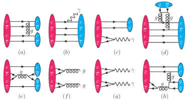
Figure 1: Typical Feynman diagrams for fully charmed tetraquark decays.

We first calculate the decay amplitude of the tetraquark states $T_{4c}$ with spin-zero and spin-two into double $J/\psi$. Two types of models are employed:

1. Model I: Quark model. The four-quark system $cc\bar{c}\bar{c}$ obeys the Pauli principle and color confinement and has no other restrictions. The form of the quark interactions is Godfrey:1985xj ,

   $$V_{ij}=V_{ij}^{conf}+V_{ij}^{coul}+V_{ij}^{SS}+V_{ij}^{LS}+V_{ij}^{T}.$$ (1)

   Specifically, there are four types of quark interactions $V_{12}$, $V_{34}$, $V_{14}$, and $V_{23}$ that drive the decay of the tetraquark state. The confinement potential $V_{ij}^{conf}$, Coulomb potential $V_{ij}^{Coul}$, spin-spin contact hyperfine potential $V_{ij}^{SS}$, spin-orbit potential $V_{ij}^{LS}$, and the tensor term $V_{ij}^{T}$ are standard in quark potential model, which can be found in the Supplemental material.

   The decay amplitude $\mathcal{M}(T_{4c}\to H_{c\bar{c}}H^{(\prime)}_{c\bar{c}})$ is given by:

   $$\mathcal{M}(T_{4c}\to H_{c\bar{c}}H^{(\prime)}_{c\bar{c}}) = -\sqrt{(2\pi)^{3}}\sqrt{8M_{T}E_{H}E_{H^{\prime}}}$$ (2)

   $$\times\left\langle H_{c\bar{c}}H^{(\prime)}_{c\bar{c}}\left|\sum_{i<j}V_{ij}\right|T_{4c}\right\rangle,$$

   where $M_{T}$ is the mass of the initial tetraquark state. $E_{H}$ and $E_{H^{\prime}}$ are the energies of the final states in the rest frame of tetraquark, respectively.

2. Model II: Heavy quark effective theory. The four-quark system $cc\bar{c}\bar{c}$ is viewed as four freely propagating point-like color sources, dressed by strongly interacting “brown muck” light degree in heavy quark limit. The short-distance and long-distance interactions are decoupled under the condition $m_{c}\gg\Lambda_{QCD}$ and then the decay amplitudes can be factorized in heavy quark effective theory Isgur:1989vq ; Falk:1990yz . The S-matrix for $T_{4c}\to H_{c\bar{c}}H^{(\prime)}_{c\bar{c}}$ can be written as

   $$\langle HH^{\prime}|S|T_{4c}\rangle$$ (3)

   $$= (-ig_{s})^{2}\int\int\mbox{d}^{4}x\mbox{d}^{4}y$$

   $$\times\langle HH^{\prime}|\mbox{T}A^{\mu}(x)A^{\nu}(y)j_{\mu}(x)j_{\nu}(y)|T_{4c}\rangle+{\cal O}(g_{s}^{4})$$

   $$= (2\pi)^{4}\delta^{4}(P_{T}-P_{H}-P_{H^{\prime}})$$

   $$\times\frac{-g^{2}_{s}C_{A}C_{F}}{p^{2}_{ex}}\langle HH^{\prime}|\mbox{T}j_{\mu}(0)j^{\mu}(0)|T_{4c}\rangle+{\cal O}(g_{s}^{4})\,,$$

   where the last line removing a factor $i(2\pi)^{4}\delta^{4}(P_{T}-P_{H}-P_{H^{\prime}})$ will give the decay amplitude. $j_{\mu}(0)=\bar{c}\gamma_{\mu}c$ is the heavy vector current. $p_{ex}$ is the typical scale in the transition process. The hadronic transition matrix $\langle HH^{\prime}|\mbox{T}j_{\mu}(0)j^{\mu}(0)|T_{4c}\rangle$ can be performed in heavy quark effective theory. We neglect possible corrections from the emission of hard gluons which may be improved in the future.

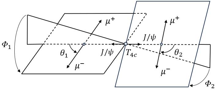
Figure 2: The illustration of helicity angles in fully charmed tetraquark decays into double $J/\psi$.

Tetraquark Cascade Decay Distribution.

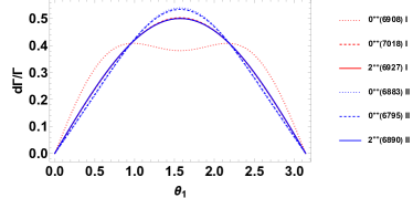
Figure 3: The polar angle $\theta_{1}$ distribution for various tetraquarks near 6.9 GeV into double $J/\psi(\to\mu^{+}+\mu^{-})$ with Quark model (I) and Heavy quark effective theroy (II). The $2^{++}$ solid curves in both two models and the $0^{++}$ dashed curve in Model I overlap closely. Here and in the following, the tetraquark masses are from the previous calculation in Quark model liu:2020eha and Heavy diquark model Zhu:2020xni . The convention for these tetraquark states can be found in the Supplemental material.

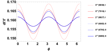
Figure 4: The plane angle $\Phi$ distribution for various tetraquarks near 6.9 GeV into double $J/\psi(\to\mu^{+}+\mu^{-})$ within different models. The $2^{++}$ solid curves in both two models overlap closely, but are well separated from $0^{++}$ curves.

The double $J/\psi$ can further decay into two pair leptons. The cascade decays shall bring more information of double $J/\psi$ exotic states. The pioneering works on the helicity amplitudes in decays can be found in Refs. Jacob:1959at ; Kramer:1991xw ; Gao:2010qx . In general, we can write the decay matrix element of the process $T_{4c}\rightarrow V_{1}+V_{2}$ in helicity base

$$\bra{V_{1}(\lambda_{1})V_{2}(\lambda_{2})}S\ket{T_{4c}(\lambda_{T})}=(2\pi)^{4}\delta^{4}(P_{T}-\sum_{i}P_{i})F^{J}_{\lambda_{1}\lambda_{2}},$$ (4)

where $\lambda_{T}$, $\lambda_{1}$ and $\lambda_{2}$ are the helicities of tetraquark and two vector mesons respectively. Then we can represent the density matrix of $T_{4c}\rightarrow V_{1}+V_{2}$ in terms of $h^{\lambda_{1}\lambda_{2}}_{\lambda_{1}^{\prime}\lambda_{2}^{\prime}}$

$$h^{\lambda_{1}\lambda_{2}}_{\lambda_{1}^{\prime}\lambda_{2}^{\prime}}=F^{J}_{\lambda_{1}\lambda_{2}}F_{\lambda_{1}^{\prime}\lambda_{2}^{\prime}}^{J*}.$$ (5)

For the decay process with two identical final particles, the helicity amplitude needs to satisfy the following symmetry

$$F^{J}_{\lambda_{1}\lambda_{2}}=(-1)^{J}F^{J}_{\lambda_{2}\lambda_{1}}.$$ (6)

Also, if parity is conserved in decay process, there is another relation between helicity amplitudes

$$F^{J}_{\lambda_{1}\lambda_{2}}=\eta\eta_{1}\eta_{2}(-1)^{J-s_{1}-s_{2}}F^{J}_{-\lambda_{1}-\lambda_{2}},$$ (7)

where $\eta$ and $\eta_{i}$ are the parity of the involving particles.

Further, $V_{1}$ two-body decays to $X_{11}+X_{12}$ while $V_{2}$ two-body decays to $X_{21}+X_{22}$. We define $\theta_{1}$ the polar angle of $X_{11}$ momentum in the rest frame of $V_{1}$ with respect to the helicity axis. Similarly, $\theta_{2}$ is the polar angle of $X_{21}$ momentum in the rest frame of $V_{2}$ with respect to the helicity axis. The angle between the two decay planes of $V_{1}$ and $V_{2}$ is defined as $\Phi=\pi-\Phi_{1}-\Phi_{2}$. The illustration of helicity angles in fully heavy tetraquark decays into two vector mesons is shown in Fig. 2.

In the case of $T_{4c}\left(0^{++}\right)\rightarrow J/\psi(\rightarrow\mu^{+}\mu^{-})+J/\psi(\rightarrow\mu^{+}\mu^{-})$, the value of $\lambda_{a}$ and $\lambda_{b}$ can be $\pm\frac{1}{2}$. We have the decay angular distribution

$$\frac{d^{3}\Gamma}{d\cos\theta_{1}d\cos\theta_{2}d\Phi}= \frac{9P_{H}}{256\pi^{2}M_{T}^{2}}\Big{\{}h^{00}_{00}\sin^{2}\theta_{1}\sin^{2}\theta_{2}$$

$$+\frac{1}{2}h^{11}_{11}(1+\cos^{2}\theta_{1})(1+\cos^{2}\theta_{2})$$

$$+\frac{1}{8}h^{11}_{11}\sin^{2}\theta_{1}\sin^{2}\theta_{2}\cos 2\Phi$$

$$+\frac{1}{4}h^{11}_{00}\sin 2\theta_{1}\sin 2\theta_{2}\cos\Phi\Big{\}}.$$ (8)

In the case of $T_{4c}\left(2^{++}\right)\rightarrow J/\psi(\rightarrow\mu^{+}\mu^{-})+J/\psi(\rightarrow\mu^{+}\mu^{-})$, there are nine combinations of $(\lambda_{1},\lambda_{2})$. The decay angular distribution becomes

$$\frac{d^{4}\Gamma}{d\cos\theta_{1}d\Phi_{1}d\cos\theta_{2}d\Phi_{2}}= \frac{45P_{H}}{1024\pi^{2}M_{T}^{2}}\Big{\{}2h_{00}^{00}+9h_{11}^{11}+12h_{-10}^{-10}+9h_{-11}^{-11}+(-2h_{00}^{00}+3h_{11}^{11}-4h_{-10}^{-10}+3h_{-11}^{-11})\cos 2\theta_{2}$$

$$+(-2h_{00}^{00}+3h_{11}^{11}-4h_{-10}^{-10}+3h_{-11}^{-11})\cos 2\theta_{1}+(2h_{00}^{00}+h_{11}^{11}-4h_{-10}^{-10}+h_{-11}^{-11})\cos 2\theta_{1}\cos 2\theta_{2}$$

$$+4h_{11}^{11}\cos(2\Phi_{1}+2\Phi_{2})\sin^{2}\theta_{1}\sin^{2}\theta_{2}+4(h_{00}^{11}-h_{-10}^{-10})\cos(\Phi_{1}+\Phi_{2})\sin 2\theta_{1}\sin 2\theta_{2})\Big{\}}.$$ (9)

Note that here we have given the simplest expression in Eqs. (Decoding spin-parity quantum numbers and decay widths of double $J/\psi$ exotic states) and (Decoding spin-parity quantum numbers and decay widths of double $J/\psi$ exotic states) under the constraints from identical nature of bosons in Eq. (6) and parity conservation in Eq. (7). Relaxing these constraints, the most general expressions of angular distribution for four-body decays are given in the Supplemental material.

Results and Discussions.

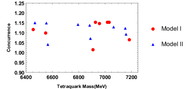
Figure 5: The concurrence of fully charmed tetraquark into double $J/\psi$ under two different theoretical models.

We calculate the decay helicity amplitudes of fully charmed tetraquark states with different spin-parity quantum numbers using two kinds of theoretical models (I and II) mentioned above. We plot the polar angle $\theta_{1}$ distribution for various tetraquarks near 6.9 GeV in Fig. 3. The polar angle $\theta_{2}$ distribution is identical to the $\theta_{1}$ distribution due to the symmetry of final two vector mesons. Similarly, we plot the distribution of plane angle $\Phi$ between the two decay planes for various tetraquarks near 6.9 GeV in Fig. 4. The distributions for other tetraquarks are given in the Supplemental material.

By combining the curve distributions in Figs. 3 and 4, fully charmed tetraquarks with different spin-parity can be distinguished. An especially important point is that we find the partial decay width of the spin-two state changes slightly with respect to the angle $\Phi$, while the two models predicting the spin-zero state exhibit a strong $\Phi$ dependence and shows significant oscillatory behavior. As for the other polar angle $\theta_{1}$ distribution, it can be further used to distinguish spin-0 states between different theoretical models.

Another characteristic property of fully charmed tetraquark decay into double $J/\psi$ is the quantum correlation between the final two $J/\psi$ mesons. Typically, to describe the quantum entanglement effects in a two-particle system, various entanglement measures can be introduced, such as the concurrence and von Neumann entropy Chen:2024syv . Here, we use concurrence to characterize the degree of quantum entanglement in fully charmed tetraquark decay process. For a state of two qutrits, the concurrence can be computed as Barr:2024djo

$$\mathcal{C}=\sqrt{2(1-\mathrm{Tr}\rho_{A}^{2})},$$ (10)

where $\rho_{A}$ represents the partial trace of the total density matrix over one of the subsystems (denoted as A). For the two qutrit system, its value satisfies $[max\left(0,LB\right),\frac{2}{\sqrt{3}}]$ Morales:2023gow ; Zhao2010 ; Eltschka2015 . The larger the value, the stronger the degree of entanglement. We plot the concurrence of fully charmed tetraquark into double $J/\psi$ under two different theoretical models in Fig. 5. We find that the concurrence of decay process of fully charmed tetraquarks with different principal quantum numbers but the same spin-parity quantum numbers is almost equal. From both models, the concurrence for the spin-two state shows a significant separation from that of the spin-zero state. These results will provide a different perspective on understanding the tetraquark structures and their decay behaviors.

Conversely, if we consider quantum entanglement as a fundamental principle in the decays, we can derive the following conclusions. The upper and lower limits on concurrence will constrain the helicity amplitudes. If we define the normalization factor to be $N=\sum_{ij}h_{ij}^{ij}$. For the tetraquark with spin 0, we have the constraint on helicity amplitudes

$$max\left(0,\sqrt{\frac{1}{3}}\left[\frac{h_{00}^{00}+2h_{01}^{01}+4h_{11}^{00}+2h_{11}^{11}}{N}-1\right]\right)\leq\sqrt{2(1-\frac{\left(h_{00}^{00}\right)^{2}+2\left(h_{11}^{11}\right)^{2}}{N^{2}})}\leq\frac{2}{\sqrt{3}}.$$ (11)

For the tetraquark with spin 2, we have the constraint

$$max\left(0,LB_{2}\right)\leq\sqrt{2(1-\left(\frac{h_{00}^{00}+2h_{10}^{10}}{N}\right)^{2}-\left(\frac{h_{10}^{10}+h_{11}^{11}+h_{1-1}^{1-1}}{N}\right)^{2}-\left(\frac{h_{10}^{10}+h_{1-1}^{1-1}+h_{11}^{11}}{N}\right)^{2})}\leq\frac{2}{\sqrt{3}}.$$ (12)

In above, some matrix elements have no complex conjugation because they are real numbers. The lower bound for the decay of tetraquark with spin 2 is complicated which can be found in the Supplemental material, where the general constraints are also given. All these constraints will assist experimentalists in fitting the angular distribution curves and extracting the helicity amplitudes using experimental data.

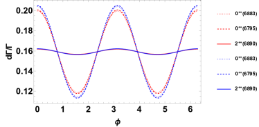
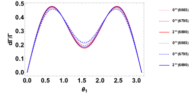
Figure 6: The $\theta_{1}$ and $\Phi$ distributions for various tetraquarks near 6.9 GeV into $D_{(s)}^{*}(\rightarrow D_{(s)}\pi)$ and $\bar{D}_{(s)}^{*}(\rightarrow\bar{D}_{(s)}\pi)$ using Model II.

In addition to fully charmed tetraquark decay into double $J/\psi$, we also need to study fully charmed tetraquark into double charmed mesons, as they collectively determine the tetraquark’s total decay width or lifetime. We only give the results from Model II, which are plotted in Fig. 6. We find that the dependence of plane angle $\Phi$ for double charmed mesons channel are similar to that for double $J/\psi$ channel, while the dependence of polar angle $\theta_{1}$ is completely different due to the difference of final products. Especially we find the curves of the spin-two state remain nearly constant with respect to the angle $\Phi$, exhibiting an independence characteristic, which may provide a supplementary plan for determining the spin-parity of double $J/\psi$ exotic states. To achieve these goals, one may consider the process, $T_{4c}\to{D^{*}}(2010)^{+}(\to D^{0}+\pi^{+})+{D^{*}}(2010)^{-}(\to\bar{D}^{0}+\pi^{-})$ along with $D^{0}\to K^{-}+\pi^{+}$, to be a favorable observation channel. Additionally, we believe this channel can be used to probe fully charmed tetraquark below the double charmonia threshold that have not yet been observed in experiment.

Conclusion. The confirmation of the completely new family of fully charmed tetraquark states is expected to play a significant role in testing the Standard Model of particle physics and advancing our understanding of the color confinement mechanism in QCD. Performing a strict calculation within both the quark model and heavy quark effective theory, we have demonstrated the feasibility of the angular distribution method to distinguish the spin and parity quantum numbers of fully charmed tetraquarks. We have also identified the main decay mechanisms for fully charmed tetraquarks, which are employed to explain the exotic double $J/\psi$ spectrum and total decay widths observed among LHCb, ATLAS and CMS experiments. The quantum entanglement effect between the two vector mesons from fully charmed tetraquark is also studied, showing that the concurrence is nearly unchanged for the decays of various radially excited tetraquark with identical $J^{PC}$, and the difference is reduced for higher excited tetraquark with different spin. The constraints formula for the helicity amplitudes are given assuming the fundamental principle of entanglement, which shall be useful for experimentalists to fit the helicity amplitudes. These results of angular distribution and partial decay widths can be tested in current particle physics experiments such as LHCb, ATLAS, CMS and Belle-II.

It is worth noting that the decays into open charm meson pair such as $D^{(*)}_{(s)}\bar{D}_{(s)}^{(*)}$ are crucial for searching for fully charmed tetraquark states below the double charmonia threshold, as these processes are the main decay modes in this case. Moreover, although the branching ratio for the two-photon channel is small, it is worth experimentally attempting to search for fully charmed tetraquark states due to its clean background. The processes mentioned above will undoubtedly provide a fresh perspective on double $J/\psi$ exotic states, helping to reveal the multi-peak structures, clarify their internal properties, and establish fully charmed tetraquark family.

I Supplemental material

In the supplemental material, we will give the calculation in both quark model and heavy quark effective theory, the derivation of angular distribution for tetraquark decays into two vector mesons. The theoretical predictions of double $J/\psi$ exotic states are compared with experimental data from LHCb, ATLAS, and CMS. The theoretical predictions of polar angle $\theta_{1}$ and decay planes angle difference $\Phi$ distributions for various tetraquarks into double $J/\psi$ and double charmed mesons are also given. Configurations for the tetraquark $cc\bar{c}\bar{c}$ system in quark model (Model I) are given in Tab. 1. The comparison of double $J/\psi$ exotic states from current experiment data and the theoretical predictions are given in Tab. 2. The major decay modes and their decay widths for fully charmed tetraquark states are given in Tab. 3. The formula for the concurrence constraint of helicity amplitudes are given in the end.

I.1 Quark model

In quark model, the confinement potential $V_{ij}^{conf}$, Coulomb potential $V_{ij}^{Coul}$, the spin-spin contact hyperfine potential $V_{ij}^{SS}$, the spin-orbit potential $V_{ij}^{LS}$, and the tensor term $V_{ij}^{T}$ are given by the following expressions

$$V_{ij}^{conf} = -\frac{3}{16}\left(\boldsymbol{\lambda}_{i}\cdot\boldsymbol{\lambda}_{j}\right)\left(b_{ij}r_{ij}\right),$$ (A.1)

$$V_{ij}^{Coul} = \frac{1}{4}\left(\boldsymbol{\lambda}_{i}\cdot\boldsymbol{\lambda}_{j}\right)\left(\frac{\alpha_{ij}}{r_{ij}}\right),$$ (A.2)

$$V_{ij}^{SS} = -\frac{\alpha_{ij}}{4}\left(\boldsymbol{\lambda}_{i}\cdot\boldsymbol{\lambda}_{j}\right)\left\{\frac{\sigma_{ij}^{3}e^{-\sigma_{ij}^{2}r_{ij}^{2}}}{\pi^{1/2}}\frac{8(\mathbf{S}_{i}\cdot\mathbf{S}_{j})}{3m_{i}m_{j}}\right\},~{}~{}~{}~{}$$ (A.3)

$$V_{ij}^{LS} = -\frac{\alpha_{ij}}{16}\frac{\left(\boldsymbol{\lambda}_{i}\cdot\boldsymbol{\lambda}_{j}\right)}{r_{ij}^{3}}\bigg{(}\frac{1}{m_{i}^{2}}+\frac{1}{m_{j}^{2}}+\frac{4}{m_{i}m_{j}}\bigg{)}LS_{+}$$ (A.4)

$$-\frac{\alpha_{ij}}{16}\frac{\left(\boldsymbol{\lambda}_{i}\cdot\boldsymbol{\lambda}_{j}\right)}{r_{ij}^{3}}\bigg{(}\frac{1}{m_{i}^{2}}-\frac{1}{m_{j}^{2}}\bigg{)}LS_{-},$$

$$V_{ij}^{T} = -\frac{\alpha_{ij}}{4}\left(\boldsymbol{\lambda}_{i}\cdot\boldsymbol{\lambda}_{j}\right)\cdot\frac{1}{m_{i}m_{j}r_{ij}^{3}}$$ (A.5)

$$\times\Bigg{\{}\frac{3(\mathbf{S}_{i}\cdot\mathbf{r}_{ij})(\mathbf{S}_{j}\cdot\mathbf{r}_{ij})}{r_{ij}^{2}}-\mathbf{S}_{i}\cdot\mathbf{S}_{j}\Bigg{\}}.$$

In the above equations, $r_{ij}\equiv|\mathbf{r}_{i}-\mathbf{r}_{j}|$ is the distance between the $i$-th and $j$-th quarks, and $\boldsymbol{\lambda}_{i,j}$ are the color operators acting on the $i,j$-th quarks. $LS_{+}=\mathbf{L}_{ij}\cdot(\mathbf{S}_{i}+\mathbf{S}_{j})$ and $LS_{-}=\mathbf{L}_{ij}\cdot(\mathbf{S}_{i}-\mathbf{S}_{j})$. $\mathbf{L}_{ij}$ represents the relative orbital angular momentum between the $i$-th and $j$-th quarks, and $\mathbf{S}_{i}$ represents the spin of the $i$-th quark. The parameters $b_{ij}$ and $\alpha_{ij}$ denote the strength of the confinement and the strong coupling of the one-gluon-exchange potential, respectively.

Table 1: Configurations for the tetraquark $cc\bar{c}\bar{c}$ system considered from quark model (Model I) in this work. Their masses are given in the last column.

Configuration	Wave Function		Mass(MeV)
$1^{1}S_{0^{++}(6\bar{6})_{c}}$	$\psi_{000}^{1S}$$\chi_{00}^{00}$	$|6\bar{6}\rangle^{c}$	6455
$1^{1}S_{0^{++}(\bar{3}3)_{c}}$	$\psi_{000}^{1S}$$\chi_{00}^{11}$	$|\bar{3}3\rangle^{c}$	6550
$1^{5}S_{2^{++}(\bar{3}3)_{c}}$	$\psi_{000}^{1S}$$\chi_{22}^{11}$	$|\bar{3}3\rangle^{c}$	6524
$2^{1}S_{0^{++}(6\bar{6})_{c}\left(\xi_{1},\xi_{2}\right)}$	$\sqrt{\frac{1}{2}}\left(\psi_{100}^{\xi_{1}}+\psi_{100}^{\xi_{2}}\right)$$\chi_{00}^{00}$	$|6\bar{6}\rangle^{c}$	6908
$2^{1}S_{0^{++}(\bar{3}3)_{c}\left(\xi_{1},\xi_{2}\right)}$	$\sqrt{\frac{1}{2}}\left(\psi_{100}^{\xi_{1}}+\psi_{100}^{\xi_{2}}\right)$$\chi_{00}^{11}$	$|\bar{3}3\rangle^{c}$	6957
$2^{1}S_{0^{++}(6\bar{6})_{c}\left(\xi_{3}\right)}$	$\psi_{100}^{\xi_{3}}$$\chi_{00}^{00}$	$|6\bar{6}\rangle^{c}$	7018
$2^{1}S_{0^{++}(\bar{3}3)_{c}\left(\xi_{3}\right)}$	$\psi_{100}^{\xi_{3}}$$\chi_{00}^{11}$	$|\bar{3}3\rangle^{c}$	7185
$2^{5}S_{2^{++}(\bar{3}3)_{c}\left(\xi_{1},\xi_{2}\right)}$	$\sqrt{\frac{1}{2}}\left(\psi_{100}^{\xi_{1}}+\psi_{100}^{\xi_{2}}\right)$$\chi_{22}^{11}$	$|\bar{3}3\rangle^{c}$	6927
$2^{5}S_{2^{++}(\bar{3}3)_{c}\left(\xi_{3}\right)}$	$\psi_{100}^{\xi_{3}}$$\chi_{22}^{11}$	$|\bar{3}3\rangle^{c}$	7032

Table 2: Double $J/\psi$ exotic states from current experiment data and the theoretical predictions based on quark model (QM) and heavy quark effective theory (HQET). Three exotic states with mass around 6.5, 6.9, 7.1 GeV in double $J/\psi$ spectrum are observed in experiments, respectively. In theoretical side, we only give the results with tetraquark spin-parity $J^{PC}=0^{++}$ and $J^{PC}=2^{++}$ to explain the experimental data. The convention for fully charmed tetraquark states in QM are listed in Tab. 1. The fully charmed tetraquark spectrum in HQET are adopted in heavy diquark model where the first three lines $0^{++}$ are from two axial-vector diquark and the following three lines $0^{++}$ are from two scalar diquark with different principle quantum numbers. The decay widths of $1S$ tetraquark states below double charmonia threshold in HQET are given in Tab. 3. The unit for mass $M_{\mathrm{BW}_{i}}(M_{T})$ and decay width $\Gamma_{\mathrm{BW}_{i}}(\Gamma_{T})$ is in MeV. The universal parameters to estimate the decay widths in HQET are roughly chosen as $\xi_{\psi}=\xi_{\eta_{c}}=\xi_{\chi_{c0}}=\xi_{h_{c}}=\xi_{D}=\xi_{D_{s}}=0.1$. The decay constants for tetraquark are roughly chosen as $f^{\prime n}_{0}=f^{n}_{0}=f^{n}_{2}=100$ MeV with $n=1,2,3,4$.

Exp.	Fit method	$M_{\mathrm{BW}_{1}}$	$\Gamma_{\mathrm{BW}_{1}}$	$M_{\mathrm{BW}_{2}}$	$\Gamma_{\mathrm{BW}_{2}}$	$M_{\mathrm{BW}_{3}}$	$\Gamma_{\mathrm{BW}_{3}}$
LHCb LHCb:2020bwg	No interf.	-	-	$6905\pm 11\pm 7$	$80\pm 19\pm 33$	-	-
LHCb LHCb:2020bwg	Interf.	$6741\pm 6$	$288\pm 16$	$6886\pm 11\pm 11$	$168\pm 33\pm 69$	-	-
ATLAS ATLAS:2023bft	Fit-A	$6630\pm 50_{-10}^{+80}$	$350\pm 110_{-40}^{+110}$	$6860\pm 30_{-20}^{+10}$	$110\pm 50_{-10}^{+20}$	$7220\pm 30_{-40}^{+10}$	$90\pm 60_{-50}^{+60}$
ATLAS ATLAS:2023bft	Fit-B	$6650\pm 20_{-20}^{+30}$	$440\pm 50_{-50}^{+60}$	$6910\pm 10\pm 10$	$150\pm 30\pm 10$	-	-
CMS CMS:2023owd	No interf.	$6552\pm 10\pm 12$	$124_{-26}^{+32}\pm 33$	$6927\pm 9\pm 4$	$122_{-21}^{+24}\pm 184$	$7287_{-18}^{+20}\pm 5$	$95_{-40}^{+59}\pm 19$
CMS CMS:2023owd	Interf.	$6638_{-38-31}^{+43+16}$	$440_{-200-240}^{+230}$	$6847_{-28-20}^{+44}$	$191_{-49-17}^{+66+25}$	$7134_{-25-15}^{+48+41}$	$97_{-29-26}^{+40+29}$
Theo.	$n,^{2S+1}L_{J},J^{PC}$	$M_{T}$	$\Gamma_{T}$	$M_{T}$	$\Gamma_{T}$	$M_{T}$	$\Gamma_{T}$
QM	1,${}^{1}S_{0},0^{++}$	6455	20.5	-	-	-	-
	1,${}^{1}S_{0},0^{++}$	6550	7.5	-	-	-	-
	1,${}^{5}S_{2},2^{++}$	6524	31.0	-	-	-	-
	2,${}^{1}S_{0},0^{++}$	-	-	6908	38.7	-	-
	2,${}^{1}S_{0},0^{++}$	-	-	6957	83.3	-	-
	2,${}^{1}S_{0},0^{++}$	-	-	-	-	7018	34.6
	2,${}^{1}S_{0},0^{++}$	-	-	-	-	7185	36.9
	2,${}^{5}S_{2},2^{++}$	-	-	6927	27.1	-	-
	2,${}^{5}S_{2},2^{++}$	-	-	-	-	7032	670.9
HQET	2,${}^{1}S_{0},0^{++}$	$6555^{+36}_{-37}$	15.5	-	-	-	-
	3,${}^{1}S_{0},0^{++}$	-	-	$6883^{+27}_{-27}$	16.2	-	-
	4,${}^{1}S_{0},0^{++}$	-	-	-	-	$7154^{+22}_{-22}$	15.9
	2,${}^{1}S_{0},0^{++}$	$6468^{+35}_{-35}$	23.6	-	-	-	-
	3,${}^{1}S_{0},0^{++}$	-	-	$6795^{+26}_{-26}$	21.3	-	-
	4,${}^{1}S_{0},0^{++}$	-	-	-	-	$7066^{+21}_{-22}$	27.1
	2,${}^{5}S_{2},2^{++}$	$6566^{+34}_{-35}$	39.4	-	-	-	-
	3,${}^{5}S_{2},2^{++}$	-	-	$6890^{+27}_{-26}$	36.0	-	-
	4,${}^{5}S_{2},2^{++}$	-	-	-	-	$7160^{+21}_{-22}$	29.0

Table 3: The major decay modes for fully charmed tetraquark included in this work. The unit for the mass and partial decay width is in MeV. Therein, $D^{(*)}\bar{D}^{(*)}$ includes $D^{*+}D^{*-}$, $D^{*0}\bar{D}^{*0}$, $D^{+}D^{-}$ and $D^{0}\bar{D}^{0}$. $H_{c}H_{c}^{\prime}$ includes all other charmonium pair modes except $J/\psi J/\psi$.

Theo.	$n,^{2S+1}L_{J},J^{PC}$,$M_{T}$	$J/\psi J/\psi$	$H_{c}H_{c}^{\prime}$	$D^{(*)}\bar{D}^{(*)}$	$D^{(*)}_{s}\bar{D}^{(*)}_{s}$	$gg$	$\gamma\gamma(\times 10^{-3})$
QPM	1,${}^{1}S_{0},0^{++},6455$	0.7	1.45	$9.6(\frac{\xi_{D}}{0.1})^{2}$	$6.9(\frac{\xi_{D_{s}}}{0.1})^{2}$	$1.9(\frac{f^{\prime 1}_{0}}{100})^{2}$	$1.3(\frac{f^{\prime 1}_{0}}{100})^{2}$
	1,${}^{1}S_{0},0^{++},6550$	1.78	0.12	$3.0(\frac{\xi_{D}}{0.1})^{2}$	$2.1(\frac{\xi_{D_{s}}}{0.1})^{2}$	$0.5(\frac{f^{1}_{0}}{100})^{2}$	$0.3(\frac{f^{1}_{0}}{100})^{2}$
	1,${}^{5}S_{2},2^{++},6524$	-	-	$15(\frac{\xi_{D}}{0.1})^{2}$	$14.2(\frac{\xi_{D_{s}}}{0.1})^{2}$	$1.8(\frac{f^{2}_{2}}{100})^{2}$	$1.3(\frac{f^{2}_{2}}{100})^{2}$
	2,${}^{1}S_{0},0^{++},6908$	0.12	23.75	$7.6(\frac{\xi_{D}}{0.1})^{2}$	$5.5(\frac{\xi_{D_{s}}}{0.1})^{2}$	$1.7(\frac{f^{\prime 2}_{0}}{100})^{2}$	$1.3(\frac{f^{\prime 2}_{0}}{100})^{2}$
	2,${}^{1}S_{0},0^{++},6957$	4.66	74.03	$2.4(\frac{\xi_{D}}{0.1})^{2}$	$1.8(\frac{\xi_{D_{s}}}{0.1})^{2}$	$0.4(\frac{f^{2}_{0}}{100})^{2}$	$0.3(\frac{f^{2}_{0}}{100})^{2}$
	2,${}^{1}S_{0},0^{++},7018$	1.87	18.01	$7.8(\frac{\xi_{D}}{0.1})^{2}$	$5.2(\frac{\xi_{D_{s}}}{0.1})^{2}$	$1.7(\frac{f^{\prime 2}_{0}}{100})^{2}$	$1.2(\frac{f^{\prime 2}_{0}}{100})^{2}$
	2,${}^{1}S_{0},0^{++},7185$	0.48	32.25	$2.2(\frac{\xi_{D}}{0.1})^{2}$	$1.6(\frac{\xi_{D_{s}}}{0.1})^{2}$	$0.4(\frac{f^{2}_{0}}{100})^{2}$	$0.3(\frac{f^{2}_{0}}{100})^{2}$
	2,${}^{5}S_{2},2^{++},6927$	0.36	1.45	$12(\frac{\xi_{D}}{0.1})^{2}$	$11.6(\frac{\xi_{D_{s}}}{0.1})^{2}$	$1.7(\frac{f^{2}_{2}}{100})^{2}$	$1.3(\frac{f^{2}_{2}}{100})^{2}$
	2,${}^{5}S_{2},2^{++},7032$	7.12	640.06	$11(\frac{\xi_{D}}{0.1})^{2}$	$11(\frac{\xi_{D_{s}}}{0.1})^{2}$	$1.7(\frac{f^{2}_{2}}{100})^{2}$	$1.2(\frac{f^{2}_{2}}{100})^{2}$
HQET	1,${}^{1}S_{0},0^{++},6055$	-	-	$4.0(\frac{\xi_{D}}{0.1})^{2}$	$2.8(\frac{\xi_{D_{s}}}{0.1})^{2}$	$2.0(\frac{f^{\prime 1}_{0}}{100})^{2}$	$1.4(\frac{f^{\prime 1}_{0}}{100})^{2}$
	1,${}^{1}S_{0},0^{++},5984$	-	-	$16.4(\frac{\xi_{D}}{0.1})^{2}$	$8.7(\frac{\xi_{D_{s}}}{0.1})^{2}$	$0.5(\frac{f^{1}_{0}}{100})^{2}$	$0.4(\frac{f^{1}_{0}}{100})^{2}$
	1,${}^{5}S_{2},2^{++},6090$	-	-	$19.3(\frac{\xi_{D}}{0.1})^{2}$	$17.6(\frac{\xi_{D_{s}}}{0.1})^{2}$	$2.0(\frac{f^{1}_{2}}{100})^{2}$	$1.4(\frac{f^{1}_{2}}{100})^{2}$
	2,${}^{1}S_{0},0^{++},6555$	$2.6(\frac{\xi_{\psi}}{0.1})^{2}$	$6.0(\frac{\xi_{\eta_{c}}}{0.1})^{2}$	$3.0(\frac{\xi_{D}}{0.1})^{2}$	$2.1(\frac{\xi_{D_{s}}}{0.1})^{2}$	$1.8(\frac{f^{\prime 2}_{0}}{100})^{2}$	$1.3(\frac{f^{\prime 2}_{0}}{100})^{2}$
	2,${}^{1}S_{0},0^{++},6468$	$5.5(\frac{\xi_{\psi}}{0.1})^{2}$	$1.2(\frac{\xi_{\eta_{c}}}{0.1})^{2}$	$9.6(\frac{\xi_{D}}{0.1})^{2}$	$6.8(\frac{\xi_{D_{s}}}{0.1})^{2}$	$0.5(\frac{f^{2}_{0}}{100})^{2}$	$0.3(\frac{f^{2}_{0}}{100})^{2}$
	2,${}^{5}S_{2},2^{++},6566$	$8.5(\frac{\xi_{\psi}}{0.1})^{2}$	$0.01(\frac{\xi_{\eta_{c}}}{0.1})^{2}$	$14.9(\frac{\xi_{D}}{0.1})^{2}$	$14(\frac{\xi_{D_{s}}}{0.1})^{2}$	$2.0(\frac{f^{2}_{2}}{100})^{2}$	$1.4(\frac{f^{2}_{2}}{100})^{2}$
	3,${}^{1}S_{0},0^{++},6883$	$3.6(\frac{\xi_{\psi}}{0.1})^{2}$	$5.7(\frac{\xi_{\eta_{c}}}{0.1})^{2}+0.8(\frac{\xi_{\chi_{c0}}}{0.1})^{2}$	$2.6(\frac{\xi_{D}}{0.1})^{2}$	$1.8(\frac{\xi_{D_{s}}}{0.1})^{2}$	$1.7(\frac{f^{\prime 3}_{0}}{100})^{2}$	$1.3(\frac{f^{\prime 3}_{0}}{100})^{2}$
	3,${}^{1}S_{0},0^{++},6795$	$6.3(\frac{\xi_{\psi}}{0.1})^{2}$	$0.7(\frac{\xi_{\eta_{c}}}{0.1})^{2}$	$8(\frac{\xi_{D}}{0.1})^{2}$	$5.9(\frac{\xi_{D_{s}}}{0.1})^{2}$	$0.4(\frac{f^{3}_{0}}{100})^{2}$	$0.3(\frac{f^{3}_{0}}{100})^{2}$
	3,${}^{5}S_{2},2^{++},6890$	$9.6(\frac{\xi_{\psi}}{0.1})^{2}$	$0.03(\frac{\xi_{\eta_{c}}}{0.1})^{2}$	$12.5(\frac{\xi_{D}}{0.1})^{2}$	$11.9(\frac{\xi_{D_{s}}}{0.1})^{2}$	$2.0(\frac{f^{3}_{2}}{100})^{2}$	$1.4(\frac{f^{3}_{2}}{100})^{2}$
	4,${}^{1}S_{0},0^{++},7154$	$4.1(\frac{\xi_{\psi}}{0.1})^{2}$	$5.3(\frac{\xi_{\eta_{c}}}{0.1})^{2}+1.8(\frac{\xi_{\chi_{c0}}}{0.1})^{2}+0.4(\frac{\xi_{h_{c}}}{0.1})^{2}$	$2.2(\frac{\xi_{D}}{0.1})^{2}$	$0.8(\frac{\xi_{D_{s}}}{0.1})^{2}$	$1.7(\frac{f^{\prime 4}_{0}}{100})^{2}$	$1.2(\frac{f^{\prime 4}_{0}}{100})^{2}$
	4,${}^{1}S_{0},0^{++},7066$	$6.2(\frac{\xi_{\psi}}{0.1})^{2}$	$0.4(\frac{\xi_{\eta_{c}}}{0.1})^{2}+4(\frac{\xi_{\chi_{c0}}}{0.1})^{2}+4(\frac{\xi_{h_{c}}}{0.1})^{2}$	$7.0(\frac{\xi_{D}}{0.1})^{2}$	$5.1(\frac{\xi_{D_{s}}}{0.1})^{2}$	$0.4(\frac{f^{4}_{0}}{100})^{2}$	$0.3(\frac{f^{4}_{0}}{100})^{2}$
	4,${}^{5}S_{2},2^{++},7160$	$9.8(\frac{\xi_{\psi}}{0.1})^{2}$	$0.04(\frac{\xi_{\eta_{c}}}{0.1})^{2}+1.4(\frac{\xi_{h_{c}}}{0.1})^{2}$	$10.9(\frac{\xi_{D}}{0.1})^{2}$	$10.3(\frac{\xi_{D_{s}}}{0.1})^{2}$	$2.0(\frac{f^{4}_{2}}{100})^{2}$	$1.4(\frac{f^{4}_{2}}{100})^{2}$

The decay amplitude $\mathcal{M}(A\to BC)$ is given by

$$\mathcal{M}(A\to BC) = -\sqrt{(2\pi)^{3}}\sqrt{8M_{A}E_{B}E_{C}}$$ (A.6)

$$\times\left\langle BC\left|\sum_{i<j}V_{ij}\right|A\right\rangle,$$

where $A$ represents the initial tetraquark state, and $BC$ represents the final hadron pair. $M_{A}$ is the mass of the initial state. The initial state mass is taken as that of the configuration before the mixing process. $E_{B}$ and $E_{C}$ are the energies of the final states $B$ and $C$, respectively. For simplicity, the wave functions of the $A$, $B$, and $C$ hadron states are parametrized in the form of a single harmonic oscillator.

Taking into account the Pauli principle and color confinement for the four-quark system $cc\bar{c}\bar{c}$, we have 4 configurations for $1S$-wave ground states, and 12 configurations for the $2S$-wave radial excitations. The spin-parity quantum numbers, notations, and wave functions for these configurations are presented in Table 1. The wave function of the final state is obtained within the $J$-$J$ coupling scheme

$$\left|BC\right\rangle = \chi_{11}^{SM_{S}}\varphi_{000}^{1}\varphi_{000}^{2}\phi\left|11\right\rangle.$$ (A.7)

We use a plane wave to describe the relative motion of the two mesons in the final state

$$\phi=\frac{1}{\left(2\pi\hbar\right)^{3/2}}e^{-i\boldsymbol{p}_{f}\cdot(\boldsymbol{r}_{f_{1}}-\boldsymbol{r}_{f_{2}})},$$

where $\boldsymbol{p}_{f}$ is the three-momentum of the mesons in the final state, and $\boldsymbol{r}_{f_{1}}$ and $\boldsymbol{r}_{f_{2}}$ are the position coordinates of the hadrons 1 and 2 in the final state. The assumption of a plane wave simplifies the treatment of the relative motion between the mesons by treating them as free particles.

Calculating the matrix elements in color and spin space is relatively straightforward. The integration of the spatial part is shown below. The spatial part of the integral is given by

$$\left\langle\varphi_{000}^{1}\left(\omega_{f_{1}}\right)\varphi_{000}^{2}\left(\omega_{f_{2}}\right)\phi\right|\hat{O}_{ij}\left|\psi_{000}^{1S}\left(\omega_{i}\right)\right\rangle$$

$$= I_{Nor}\int\hat{O}e^{-\sum_{i,j}A_{ij}\boldsymbol{\xi}_{i}\cdot\boldsymbol{\xi}_{j}}e^{-i\boldsymbol{p}_{f}\cdot\boldsymbol{\xi}_{3}}\left(Y_{00}\right)^{5}d^{3}\boldsymbol{\xi}_{1}d^{3}\boldsymbol{\xi}_{2}d^{3}\boldsymbol{\xi}_{3},$$

where $\hat{O}_{ij}$ stands for the spatial-dependent operator, and $I_{Nor}$ is a normalization factor independent of the integration variables. In the calculations, the plane wave should be expanded as

$$e^{i\boldsymbol{P}\cdot\boldsymbol{r}}=\sum_{l=0}^{\infty}\sqrt{4\pi(2l+1)}i^{l}j_{l}(Pr)Y_{l0}(\hat{\boldsymbol{r}}),$$ (A.9)

where the momentum $P$ is assumed to be along the $z$ direction. With the above steps, the integration of the spatial part can be obtained.

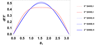
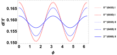
Figure 7: The $\theta_{1}$ and $\Phi$ distributions for various tetraquarks near 6.5GeV into double $J/\psi(\to\mu^{+}+\mu^{-})$within different models.

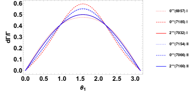
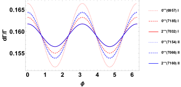
Figure 8: The $\theta_{1}$ and $\Phi$ distributions for various tetraquarks near 7.1GeV into double $J/\psi(\to\mu^{+}+\mu^{-})$ within different models.

I.2 Heavy quark effective theory

In heavy quark effective theory, the light (gluon and light quarks) Lagrangian is identical to that in QCD Lagrangian. The heavy flavor quark part of QCD Lagrangian is

$$\mathcal{L}^{Q}_{\mathrm{QCD}}= \bar{\Psi}(i\gamma^{\mu}D_{\mu}-M)\Psi,$$ (A.10)

where the heavy quark mass is expressed as $M=m_{Q}$. The covariant derivative is $D_{\mu}=\partial_{\mu}+igA_{\mu}$. If we perform the transformation of heavy quark fields with

$$\Psi= e^{-iMt}\left(\begin{array}[]{c}\psi\\ \chi\end{array}\right),$$ (A.13)

then the heavy flavor quark part of QCD Lagrangian becomes

$$\mathcal{L}^{Q}_{\mathrm{HQET}}= \left(\begin{array}[]{cc}\psi^{\dagger}&-\chi^{\dagger}\end{array}\right)\left(i\gamma^{\mu}D_{\mu}-(\gamma^{0}-1)M\right)\left(\begin{array}[]{c}\psi\\ \chi\end{array}\right)$$ (A.17)

$$= \psi^{\dagger}\left(\begin{array}[]{ll}1&\frac{i\sigma^{i}D_{i}}{iD_{t}+2M}\end{array}\right)\left(\begin{array}[]{cc}iD_{t}&i\sigma^{j}D_{j}\\ -i\sigma^{j}D_{j}&-iD_{t}-2M\end{array}\right)$$ (A.21)

$$\times\left(\begin{array}[]{c}1\\ \frac{-i\sigma^{k}D_{k}}{iD_{t}+2M}\end{array}\right)\psi$$ (A.24)

$$= \psi^{\dagger}iD_{t}\psi+\frac{1}{2M}\psi^{\dagger}\sigma^{i}D_{i}\sigma^{j}D_{j}\psi$$

$$-\frac{i}{4M^{2}}\psi^{\dagger}\sigma^{i}D_{i}D_{t}\sigma^{j}D_{j}\psi+\mathcal{O}\left(1/M^{3}\right),$$ (A.25)

where $\chi=\left(-i\sigma^{i}D_{i}\right)/\left(iD_{t}+2M\right)\psi$ are employed from the Dirac equation.

In above, we successfully decoupled the heavy quark field from QCD. Similarly, we can get the heavy antiquark effective Lagrangian. If we perform the transformation of heavy quark fields with

$$\Psi=e^{iMt}\left(\begin{array}[]{c}\psi\\ \chi\end{array}\right),$$ (A.28)

then the heavy antiquark part of QCD Lagrangian becomes

$$\mathcal{L}^{\bar{Q}}_{\mathrm{HQET}}= \left(\begin{array}[]{cc}\psi^{\dagger}&-\chi^{\dagger}\end{array}\right)\left(i\gamma^{\mu}D_{\mu}-(\gamma^{0}+1)M\right)\left(\begin{array}[]{c}\psi\\ \chi\end{array}\right)$$ (A.32)

$$= \chi^{\dagger}\left(\begin{array}[]{ll}\frac{i\sigma^{i}D_{i}}{-iD_{t}+2M}&-1\end{array}\right)\left(\begin{array}[]{cc}iD_{t}-2M&i\sigma^{j}D_{j}\\ -i\sigma^{j}D_{j}&-iD_{t}\end{array}\right)$$ (A.36)

$$\times\left(\begin{array}[]{c}\frac{i\sigma^{k}D_{k}}{-iD_{t}+2M}\\ 1\end{array}\right)\chi$$ (A.39)

$$= \chi^{\dagger}iD_{t}\chi-\frac{1}{2M}\chi^{\dagger}\sigma^{i}D_{i}\sigma^{j}D_{j}\chi$$

$$+\frac{i}{4M^{2}}\chi^{\dagger}\sigma^{i}D_{i}D_{t}\sigma^{j}D_{j}\chi+\mathcal{O}\left(1/M^{3}\right),$$ (A.40)

where $\psi=\left(-i\sigma^{i}D_{i}\right)/\left(-iD_{t}+2M\right)\chi$ are employed from the Dirac equation. Thus the heavy quark effective theory Lagrangian can be written as

$$\mathcal{L}_{\mathrm{HQET}}= \mathcal{L}^{Q}_{\mathrm{HQET}}+\mathcal{L}^{\bar{Q}}_{\mathrm{HQET}}.$$ (A.41)

In this Lagrangian, the interactions above the energy scale at heavy quark mass are integrated out and then the short-distance and long-distance interactions can be factorized. Besides the Lagrangian for two heavy quarks in nonrelativistic QCD (NRQCD) effective theory can be also obtained.

The S-matrix for $T_{4c}\to H_{c\bar{c}}H^{(\prime)}_{c\bar{c}}$ can be written as

$$\langle HH^{\prime}|S|T_{4c}\rangle$$

$$= (-ig_{s})^{2}\int\int\mbox{d}^{4}x\mbox{d}^{4}y$$

$$\times\langle HH^{\prime}|\mbox{T}A^{\mu}(x)A^{\nu}(y)j_{\mu}(x)j_{\nu}(y)|T_{4c}\rangle+{\cal O}(g_{s}^{4})$$

$$= (-ig_{s})^{2}C_{A}C_{F}\int\int\mbox{d}^{4}x\mbox{d}^{4}y\int\frac{\mbox{d}^{4}k}{(2\pi)^{4}}\frac{e^{-ik\cdot(x-y)}}{k^{2}+i0}$$

$$\times\langle HH^{\prime}|\mbox{T}j_{\mu}(x)j^{\mu}(y)|T_{4c}\rangle+{\cal O}(g_{s}^{4})$$

$$= (2\pi)^{4}\delta^{4}(P_{T}-P_{H}-P_{H^{\prime}})$$

$$\times\frac{-g^{2}_{s}C_{A}C_{F}}{(p_{i}-p_{k})^{2}+i0}\langle HH^{\prime}|\mbox{T}j_{\mu}(0)j^{\mu}(0)|T_{4c}\rangle+{\cal O}(g_{s}^{4})$$

$$= i(2\pi)^{4}\delta^{4}(P_{T}-P_{H}-P_{H^{\prime}})\mathcal{M}(T_{4c}\to H_{c\bar{c}}H^{(\prime)}_{c\bar{c}})\,,$$

where $j_{\mu}(0)=\bar{c}\gamma_{\mu}c$ is the heavy vector current. $p_{i}-p_{k}$ is the exchange momentum in the transition process.

In general, the form factors for a heavy hadron to another heavy hadron can be well-factorized among short-distance and long-distance interactions. The heavy quark part matrix elements are decoupled to the light part matrix elements as

$$\left\langle H^{\prime}\left(v^{\prime}\right)\right|J(q)|H(v)\rangle$$

$$= \left\langle Q^{\prime}\left(v^{\prime}\right),\pm\frac{1}{2}|J(q)|Q(v),\pm\frac{1}{2}\right\rangle$$

$$\times\left\langle\text{light},v^{\prime},j^{\prime},m_{j}^{\prime}|\text{light},v,j,m_{j}\right\rangle.$$ (A.43)

In heavy quark symmetry, the lowest-lying spin singlet and triplet can be described by $4\times 4$ matrices

$$H(v) =\frac{1+v\!\!\!/}{2}[i{\psi}^{\beta}\gamma_{\beta}+{\eta_{c}}\gamma^{5}]\,,$$ (A.44)

where $H_{v}$ satisfies the relation $v\!\!\!/H(v)=H(v)=-H(v)v\!\!\!/$.

Similarly, the hadronic transition matrix $\langle HH^{\prime}|\mbox{T}j_{\mu}(0)j^{\mu}(0)|T_{4c}\rangle$ can be performed in heavy quark effective theory

$$\langle HH^{\prime}|\mbox{T}j_{\mu}(0)j^{\mu}(0)|T_{4c}\rangle$$

$$\propto {\rm Tr}[\xi\,\Pi_{i}\gamma^{\mu}H^{\prime}(v^{\prime})\Pi_{j}H(v)\Gamma_{\mu}]+\ldots\,.$$ (A.45)

The decay constants for the S-wave fully charmed tetraquarks can be defined as

$$\left\langle 0\left|{\cal P}^{0^{\prime},bcde}_{\mu\nu}\psi_{b}^{\mathrm{T}}(x)C\gamma_{5}\psi_{c}(x)\bar{\psi}_{d}(x)\gamma_{5}C\bar{\psi}_{e}^{\mathrm{T}}(x)\right|T^{0^{\prime}}_{4c}(nS)\right\rangle$$

$$=if^{\prime n}_{0},$$ (A.46)

$$\left\langle 0\left|{\cal P}^{0,bcde}_{\mu\nu}\psi_{b}^{\mathrm{T}}(x)C\gamma^{\mu}\psi_{c}(x)\bar{\psi}_{d}(x)\gamma^{\nu}C\bar{\psi}_{e}^{\mathrm{T}}(x)\right|T^{0}_{4c}(nS)\right\rangle$$

$$=if^{n}_{0},$$ (A.47)

$$\left\langle 0\left|{\cal P}^{2,bcde}_{\alpha\beta\mu\nu}\psi_{b}^{\mathrm{T}}(x)C\gamma^{\mu}\psi_{c}(x)\bar{\psi}_{d}(x)\gamma^{\nu}C\bar{\psi}_{e}^{\mathrm{T}}(x)\right|T^{2}_{4c}(nS)\right\rangle$$

$$=if^{n}_{2}\varepsilon_{\alpha\beta},$$ (A.48)

where the charge conjugate operator is $C=i\gamma^{2}\gamma^{0}$.

If the initial particle has spin quantum number, $h^{\lambda_{1}\lambda_{2}}_{\lambda_{1}^{\prime}\lambda_{2}^{\prime}}$ has to be replaced by

I.3 Angular distribution

According to the Jacob-Wick theory, the angular distribution $W(\theta_{1},\theta_{2},\Phi_{1},\Phi_{2})$ can be written as

$$W(\theta_{1},\theta_{2},\Phi_{1},\Phi_{2})=\sum_{\lambda_{i}\lambda_{i}^{\prime}}H^{\lambda_{1}\lambda_{2}}_{\lambda_{1}^{\prime}\lambda_{2}^{\prime}}A_{\lambda_{1}\lambda_{1}^{\prime}}(\theta_{1},\Phi_{1})B_{\lambda_{2}\lambda_{2}^{\prime}}(\theta_{2},\Phi_{2}),$$ (A.49)

where $A_{\lambda_{1}\lambda_{1}^{\prime}}$ and $B_{\lambda_{2}\lambda_{2}^{\prime}}$ stand for the density matrix for the decays of $V_{1}$ and $V_{2}$. In general, $H^{\lambda_{1}\lambda_{2}}_{\lambda_{1}^{\prime}\lambda_{2}^{\prime}}$ has the expression

$$H^{\lambda_{1}\lambda_{2}}_{\lambda_{1}^{\prime}\lambda_{2}^{\prime}}=\sum_{\lambda_{T}}f_{\lambda_{T}}d_{\lambda_{T}\lambda}(\theta)d_{\lambda_{T}\lambda^{\prime}}(\theta)F_{\lambda_{1}\lambda_{2}}^{J}F_{\lambda_{1}^{\prime}\lambda_{2}^{\prime}}^{J*},$$ (A.50)

where $f_{\lambda_{T}}$ represents the polarization distribution relying on the production mechanism. For spin-zero initial particle, the polarization distribution satisfies $f_{0}=1$ and the $d$ function associated with $\theta$ can also be 1. In this case, we have

$$H^{\lambda_{1}\lambda_{2}}_{\lambda_{1}^{\prime}\lambda_{2}^{\prime}}=F_{\lambda_{1}\lambda_{2}}^{J}F_{\lambda_{1}^{\prime}\lambda_{2}^{\prime}}^{J*}=h^{\lambda_{1}\lambda_{2}}_{\lambda_{1}^{\prime}\lambda_{2}^{\prime}}.$$ (A.51)

And we only need one of the angles of $\Phi_{1}$ and $\Phi_{2}$ to describe the angular distribution. For unpolarized particles with spin, all polarization branching ratios take the same value. In this work, the process of particle production is not considered, so the non-polarized initial state is assumed.

Taking $A_{\lambda_{1}\lambda_{1}^{\prime}}$ as an example, it can be expressed as

$$A_{\lambda_{1}\lambda_{1}^{\prime}}(\theta_{1},\Phi_{1})=\frac{\sum_{\lambda_{a}\lambda_{b}}R_{\lambda_{1}\lambda_{1}^{\prime}}(\theta_{1},\Phi_{1},\lambda_{a},\lambda_{b})}{\sum_{\lambda_{a}\lambda_{b}}|T(p_{cm},\lambda_{a},\lambda_{b})|^{2}}.$$ (A.52)

In above, $\lambda_{a}$, $\lambda_{b}$ denote the helicity of $X_{11}$, $X_{12}$. $|T(p_{cm},\lambda_{a},\lambda_{b})|^{2}$ is the reduced matrix element for the decay of $V_{1}$, where $p_{cm}$ is the magnitude of momentum $X_{11}$ in the rest frame of $V_{1}$. $R_{\lambda_{1}\lambda_{1}^{\prime}}(\theta_{1},\lambda_{a},\lambda_{b})$ is the angular distribution for the decay of $V_{1}$ which is defined as

$$R_{\lambda_{1}\lambda_{1}^{\prime}}(\theta_{1},\lambda_{a},\lambda_{b})= \frac{2J+1}{4\pi}|T(p_{cm},\lambda_{a},\lambda_{b})|^{2}$$

$$\times D^{J*}_{\lambda_{1},\lambda_{a}-\lambda_{b}}(\Phi_{1},\theta_{1},-\Phi_{1})$$

$$\times D^{J}_{\lambda_{1}^{\prime},\lambda_{a}-\lambda_{b}}(\Phi_{1},\theta_{1},-\Phi_{1}).$$ (A.53)

$D^{J}_{m,m^{\prime}}(\alpha,\beta,\gamma)=e^{-im\alpha}d^{J}_{m,m^{\prime}}(\beta)e^{-im^{\prime}\gamma}$ is known as Wigner D matrix. The definition of $B_{\lambda_{2}\lambda_{2}^{\prime}}(\theta_{2},\Phi_{2})$ is the same as $A_{\lambda_{1}\lambda_{1}^{\prime}}(\theta_{1},\Phi_{1})$.

In the quark model, we convert the partial-wave amplitude to the helicity amplitude. Therefore, we give the relationship between the two amplitudes. For partial wave amplitudes $a_{ls}^{J}$ and helicity amplitudes $F^{J}_{\lambda_{1}\lambda_{2}}$, the relationship between the two can be expressed by the formula

$$F^{J}_{\lambda_{1}\lambda_{2}}=\sum_{ls}\sqrt{\frac{2l+1}{2J+1}}a^{J}_{ls}\langle l0s\lambda|J\lambda\rangle\langle s_{1}\lambda_{1}s_{2}-\lambda_{2}|s\lambda\rangle.$$ (A.54)

In the above formula, $l$ represents the orbital angular momentum quantum number and $s$ represents the total spin of the two daughter particles.

In the second model, we obtain the helicity amplitude directly by extracting the coefficient by writing the helicity amplitude in the form of Lorenz invariants. For a particle with spin 0, its decay amplitude can be expressed as

$$\mathcal{M}(0^{++})=\epsilon_{1\mu}^{*}\epsilon_{2\nu}^{*}\left(ag^{\mu\nu}+\frac{bp^{\mu}_{1}p^{\nu}_{2}}{m_{1}m_{2}}+\frac{ic\epsilon^{\mu\nu\alpha\beta}p_{1\alpha}p_{\beta}}{m_{1}m_{2}}\right),$$ (A.55)

where $m_{i}$, $p_{i}$ and $\epsilon_{i}$ are the mass, momentum and polarization vector for the two daughter particles, respectively. The relationship between the parameters a,b,c and the helicity amplitude can be expressed as

$$F^{0}_{11}=a+\sqrt{x^{2}-1}c,~{}~{}F^{0}_{-1-1}=a-\sqrt{x^{2}-1}c,$$

$$F^{0}_{00}=-ax-b(x^{2}-1),$$ (A.56)

where

$$x^{2}=\frac{p_{m}^{2}M_{T}^{2}}{m_{1}^{2}m_{2}^{2}}+1.$$ (A.57)

In the above formula, $p_{m}$ represents the momentum of the decaying particle in the rest frame of the parent particle and $M_{T}$ represents the mass of the parent particle.

For a particle with spin 2, its decay amplitude can be written as

$$\mathcal{M}(2^{++})= \epsilon_{1}^{*\mu}\epsilon_{2}^{*\nu}[c_{1}p_{1}\cdot p_{2}\epsilon_{3\mu\nu}+c_{2}g_{\mu\nu}\epsilon_{3\alpha\beta}\tilde{p}^{\alpha}\tilde{p}^{\beta}$$

$$+c_{3}\frac{p_{2\mu}p_{1\nu}}{M_{T}^{2}}\epsilon_{3\alpha\beta}\tilde{p}^{\alpha}\tilde{p}^{\beta}+c_{5}\epsilon_{3\alpha\beta}\frac{\tilde{p}^{\alpha}\tilde{p}^{\beta}}{M_{T}^{2}}\epsilon_{\mu\nu\rho\sigma}p_{1}^{\rho}p_{2}^{\sigma}$$

$$+2c_{4}(p_{1\nu}p_{2}^{\alpha}\epsilon_{3\mu\alpha}+p_{2\mu}p_{1}^{\alpha}\epsilon_{3\nu\alpha})$$

$$+\frac{c_{7}\epsilon_{3}^{\alpha\beta}\tilde{p}_{\beta}}{M^{2}}\left(\epsilon_{\alpha\mu\rho\sigma}p^{\rho}\tilde{p}^{\sigma}p_{\nu}+\epsilon_{\alpha\nu\rho\sigma}p^{\rho}\tilde{p}^{\sigma}p_{\mu}\right)$$

$$+c_{6}\epsilon_{3}^{\alpha\beta}\tilde{p}_{\beta}\epsilon_{\mu\nu\alpha\rho}p^{\rho}],$$ (A.58)

where $\epsilon_{3}$ represents the polarization tensor of a tensor particle and $\tilde{p}=p_{1}-p_{2}$. Considering the case of decay to two identical particles, the relationship between helicity amplitude and coefficient $c_{i}$ can be obtained by the following formula

$$F^{2}_{1-1}=F^{2}_{-11}=\frac{M_{T}^{2}}{4}c_{1}\left(1+\beta^{2}\right),$$ (A.59)

$$F^{2}_{11}=\frac{M_{T}^{2}}{\sqrt{6}}\left[\frac{c_{1}}{4}\left(1+\beta^{2}\right)+2c_{2}\beta^{2}+i\beta\left(c_{5}\beta^{2}-2c_{6}\right)\right],$$ (A.60)

$$F^{2}_{-1-1}=\frac{M_{T}^{2}}{\sqrt{6}}\left[\frac{c_{1}}{4}\left(1+\beta^{2}\right)+2c_{2}\beta^{2}-i\beta\left(c_{5}\beta^{2}-2c_{6}\right)\right],$$ (A.61)

$$F^{2}_{10}=F^{2}_{01}=\frac{M_{T}^{3}}{m\sqrt{2}}\left[\frac{c_{1}}{8}\left(1+\beta^{2}\right)+\frac{c_{4}}{2}\beta^{2}-\frac{c_{6}+c_{7}\beta^{2}}{2}i\beta\right],$$ (A.62)

$$F^{2}_{-10}=F^{2}_{0-1}=F^{2}_{10}+\frac{2M_{T}^{3}}{m\sqrt{2}}\left[\frac{c_{6}+c_{7}\beta^{2}}{2}i\beta\right],$$ (A.63)

$$F^{2}_{00}=\frac{M_{T}^{4}}{m^{2}\sqrt{6}}\left[\left(1+\beta^{2}\right)\left(\frac{c_{1}}{8}-\frac{c_{2}}{2}\beta^{2}\right)-\beta^{2}\left(\frac{c_{3}}{2}\beta^{2}-c_{4}\right)\right],$$ (A.64)

where $m$ stands for the mass of the daughter particle and $\beta=\sqrt{\frac{1-4m^{2}}{M_{T}^{2}}}$.

In the case of $T_{4c}\left(0^{++}\right)\rightarrow D^{*}(\rightarrow D\pi)+\bar{D}^{*}(\rightarrow\bar{D}\pi)$, it is obviously that $\lambda_{a}=\lambda_{b}=0$. So the decay angular distribution is

$$\frac{d^{3}\Gamma}{d\cos\theta_{1}d\cos\theta_{2}d\Phi}=\frac{9P_{D^{*}}}{64\pi^{2}M_{T}^{2}} \Big{\{}\cos^{2}\theta_{1}\cos^{2}\theta_{2}h^{00}_{00}+\frac{1}{4}\sin^{2}\theta_{1}\sin^{2}\theta_{2}(h^{11}_{11}+h^{-1-1}_{-1-1})$$

$$+\frac{1}{2}\sin^{2}\theta_{1}\sin^{2}\theta_{2}[\cos 2\Phi Re(h^{11}_{-1-1})-\sin 2\Phi Im(h^{11}_{-1-1})]$$

$$+\frac{1}{4}\sin 2\theta_{1}\sin 2\theta_{2}[\cos\Phi Re(h^{1}_{0}+h^{-1-1}_{00})-\sin\Phi Im(h^{11}_{00}-h^{-1-1}_{00})]\Big{\}}.$$ (A.65)

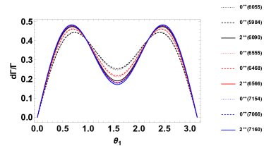
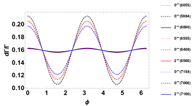
Figure 9: The $\theta_{1}$ and $\Phi$ distributions for various tetraquarks around 6.1 GeV, 6.5 GeV and 7.1 GeV into $D^{*}(\rightarrow D\pi)$ and $\bar{D}^{*}(\rightarrow\bar{D}\pi)$ using Model II.

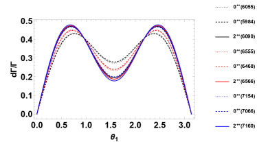
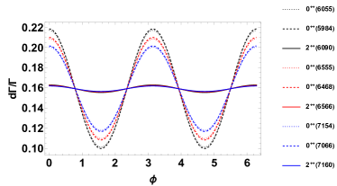
Figure 10: The $\theta_{1}$ and $\Phi$ distributions for various tetraquarks around 6.1 GeV, 6.5 GeV and 7.1 GeV into $D_{s}^{*}(\rightarrow D_{s}\pi)$ and $\bar{D}_{s}^{*}(\rightarrow\bar{D}_{s}\pi)$ using Model II.

Similarly, the decay angular distribution of $T_{4c}\left(0^{++}\right)\rightarrow J/\psi(\mu^{+}\mu^{-})+J/\psi(\mu^{+}\mu^{-})$ is

$$\frac{d^{3}\Gamma}{d\cos\theta_{1}d\cos\theta_{2}d\Phi}=\frac{9P_{H}}{256\pi^{2}M_{T}^{2}} \Big{\{}\sin^{2}\theta_{1}\sin^{2}\theta_{2}h^{00}_{00}+\frac{1}{4}(1+\cos^{2}\theta_{1})(1+\cos^{2}\theta_{2})(h^{11}_{11}+h^{-1-1}_{-1-1})$$

$$+\frac{1}{8}\sin^{2}\theta_{1}\sin^{2}\theta_{2}[\cos 2\Phi Re(h^{11}_{-1-1})-\sin 2\Phi Im(h^{11}_{-1-1})]$$

$$+\frac{1}{8}\sin 2\theta_{1}\sin 2\theta_{2}[\cos\Phi Re(h^{11}_{00}+h^{-1-1}_{00})-\sin\Phi Im(h^{11}_{00}-h^{-1-1}_{00})]\Big{\}}.$$ (A.66)

In the case of $T_{4c}\left(2^{++}\right)\rightarrow D^{*}(\rightarrow D\pi)+\bar{D}^{*}(\rightarrow\bar{D}\pi)$, the angular distribution is

$$\frac{d\Gamma}{d\cos\theta_{1}d\Phi_{1}d\cos\theta_{2}d\Phi_{2}d\cos\theta}= \frac{45P_{D^{*}}}{128M_{T}^{2}\pi^{2}}\Big{\{}[2\cos^{2}\theta_{1}\cos^{2}\theta_{2}H^{00}_{00}+\frac{1}{2}\sin^{2}\theta_{1}\sin^{2}\theta_{2}(H^{11}_{11}+H^{-1-1}_{-1-1}+H^{1-1}_{1-1}+H^{-11}_{-11})$$

$$+\sin^{2}\theta_{1}\cos^{2}\theta_{2}(H^{10}_{10}+H^{-10}_{-10})+\cos^{2}\theta_{1}\sin^{2}\theta_{2}(H^{01}_{01}+H^{0-1}_{0-1})]$$

$$+\frac{1}{2}\sin 2\theta_{1}\sin 2\theta_{2}[cos(\Phi_{1}-\Phi_{2})Re(H^{01}_{01}+H^{0-1}_{0-1}-H^{1-1}_{00}-H^{00}_{-11})-\sin(\Phi_{1}-\Phi_{2})$$

$$Im(H^{01}_{01}+H^{0-1}_{0-1}-H^{1-1}_{00}-H^{00}_{-11})+cos(\Phi_{1}+\Phi_{2})Re(H^{11}_{00}+H^{00}_{-1-1}-H^{10}_{0-1}-H^{01}_{-10})$$

$$-\sin(\Phi_{1}+\Phi_{2})Im(H^{11}_{00}+H^{00}_{-1-1}-H^{10}_{0-1}-H^{01}_{-10})]$$

$$-2\sin^{2}\theta_{1}\cos^{2}\theta_{2}[\cos 2\Phi_{1}Re(H^{10}_{-10})-\sin 2\Phi_{1}Im(H^{10}_{-10})]$$

$$-2\cos^{2}\theta_{1}\sin^{2}\theta_{2}[\cos 2\Phi_{2}Re(H^{01}_{0-1})-\sin 2\Phi_{2}Im(H^{01}_{0-1})]$$

$$+\sqrt{2}\sin 2\theta_{1}\cos^{2}\theta_{2}[\cos\Phi_{1}Re(H^{00}_{-10}-H^{10}_{00})-\sin\Phi_{1}Im(H^{00}_{-10}-H^{10}_{00})]$$

$$+\sqrt{2}\cos^{2}\theta_{1}\sin 2\theta_{2}[\cos\Phi_{2}Re(H^{00}_{0-1}-H^{01}_{00})-\sin\Phi_{2}Im(H^{00}_{0-1}-H^{01}_{00})]$$

$$+\frac{1}{\sqrt{2}}\sin 2\theta_{1}\sin^{2}\theta_{2}[\cos\Phi_{1}Re(H^{0-1}_{-1-1}+H^{01}_{-11}-H^{11}_{01}-H^{1-1}_{0-1})-\sin\Phi_{1}Im(H^{0-1}_{-1-1}$$

$$+H^{01}_{-11}-H^{11}_{01}-H^{1-1}_{0-1})+\cos(\Phi_{1}+2\Phi_{2})Re(H^{11}_{0-1}-H^{01}_{-1-1})-\sin(\Phi_{1}+2\Phi_{2})$$

$$Im(H^{11}_{0-1}-H^{01}_{-1-1})+\cos(\Phi_{1}-2\Phi_{2})Re(H^{1-1}_{01}-H^{0-1}_{-11})$$

$$-\sin(\Phi_{1}-2\Phi_{2})Im(H^{1-1}_{01}-H^{0-1}_{-11})]$$

$$+\frac{1}{\sqrt{2}}\sin^{2}\theta_{1}\sin 2\theta_{2}[\cos\Phi_{2}Re(H^{-10}_{-1-1}+H^{10}_{1-1}-H^{-11}_{-10}-H^{11}_{10})-\sin\Phi_{2}Im(H^{-10}_{-1-1}$$

$$+H^{10}_{1-1}-H^{-11}_{-10}-H^{11}_{10})+\cos(2\Phi_{1}+\Phi_{2})Re(H^{11}_{-10}-H^{10}_{-1-1})-\sin(2\Phi_{1}+\Phi_{2})$$

$$Im(H^{11}_{-10}-H^{10}_{-1-1})+\cos(2\Phi_{1}-\Phi_{2})Re(H^{10}_{-11}-H^{1-1}_{-10})$$

$$-\sin(2\Phi_{1}-\Phi_{2})Im(H^{10}_{-11}-H^{1-1}_{-10})]$$

$$+\sin^{2}\theta_{1}\sin^{2}\theta_{2}[\cos(2\Phi_{1}+2\Phi_{2})Re(H^{11}_{-1-1})-\sin(2\Phi_{1}+2\Phi_{2})Im(H^{11}_{-1-1})$$

$$+\cos 2\Phi_{1}Re(-H^{11}_{-11}-H^{1-1}_{-1-1})-\sin 2\Phi_{1}Im(-H^{11}_{-11}-H^{1-1}_{-1-1})$$

$$+\cos 2\Phi_{2}Re(-H^{11}_{1-1}-H^{-11}_{-1-1})-\sin 2\Phi_{2}Im(-H^{11}_{1-1}-H^{-11}_{-1-1})$$

$$+\cos(2\Phi_{1}-2\Phi_{2})Re(H^{1-1}_{-11})-\sin(2\Phi_{1}-2\Phi_{2})Im(H^{1-1}_{-11})]\Big{\}}.$$ (A.67)

In the case of $T_{4c}\left(2^{++}\right)\rightarrow J/\psi(\mu^{+}\mu^{-})+J/\psi(\mu^{+}\mu^{-})$, the angular distribution is

$$\frac{d\Gamma}{d\cos\theta_{1}d\Phi_{1}d\cos\theta_{2}d\Phi_{2}d\theta}= \frac{45P_{H}}{512\pi^{2}M_{T}^{2}}\Big{\{}2\sin^{2}\theta_{1}\sin^{2}\theta_{2}H^{00}_{00}+\frac{1}{2}(1+\cos^{2}\theta_{1})(1+\cos^{2}\theta_{2})(H^{-1-1}_{-1-1}+H^{11}_{11}+H^{1-1}_{1-1}$$

$$+H^{-11}_{-11})+(1+\cos^{2}\theta_{1})\sin^{2}\theta_{2}(H^{10}_{10}+H^{-10}_{-10})+\sin^{2}\theta_{1}(1+\cos^{2}\theta_{2})(H^{01}_{01}+H^{0-1}_{0-1})$$

$$+\frac{1}{2}\sin 2\theta_{1}\sin 2\theta_{2}[\cos(\Phi_{1}-\Phi_{2})Re(H^{10}_{01}+H^{0-1}_{-10}-H^{1-1}_{00}-H^{00}_{-11})-\sin(\Phi_{1}-\Phi_{2})$$

$$Im(H^{10}_{01}+H^{0-1}_{-10}-H^{1-1}_{00}-H^{00}_{-11})+\cos(\Phi_{1}+\Phi_{2})Re(H^{11}_{00}+H^{00}_{-1-1}-H^{10}_{0-1}-H^{01}_{-10})$$

$$-\sin(\Phi_{1}+\Phi_{2})Im(H^{11}_{00}+H^{00}_{-1-1}-H^{10}_{0-1}-H^{01}_{-10})]$$

$$+\frac{1}{\sqrt{2}}\sin 2\theta_{1}(1+\cos^{2}\theta_{2})[\cos\Phi_{1}Re(H^{1-1}_{0-1}+H^{11}_{01}-H^{0-1}_{-1-1}-H^{01}_{-11})-\sin\Phi_{1}$$

$$Im(H^{1-1}_{0-1}+H^{11}_{01}-H^{0-1}_{-1-1}-H^{01}_{-11})]$$

$$+\frac{1}{\sqrt{2}}(1+\cos^{2}\theta_{1})\sin 2\theta_{2}[\cos\Phi_{2}Re(H^{11}_{10}+H^{-11}_{-10}-H^{-10}_{-1-1}-H^{10}_{1-1})-\sin\Phi_{2}$$

$$Im(H^{11}_{10}+H^{-11}_{-10}-H^{-10}_{-1-1}-H^{10}_{1-1})]$$

$$+\frac{1}{\sqrt{2}}\sin^{2}\theta_{1}\sin 2\theta_{2}[\cos(2\Phi_{1}+\Phi_{2})Re(H^{11}_{-10}-H^{10}_{-1-1})-\sin(2\Phi_{1}+\Phi_{2})Im(H^{11}_{-10}$$

$$-H^{10}_{-1-1})+\cos\Phi_{2}Re(2H^{01}_{00}-2h^{00}_{0-1})-\sin\Phi_{2}Im(2H^{01}_{00}-2h^{00}_{0-1})+\cos(2\Phi_{1}-\Phi_{2})$$

$$Re(H^{10}_{-11}-H^{1-1}_{-10})-\sin(2\Phi_{1}-\Phi_{2})Im(H^{10}_{-11}-H^{1-1}_{-10})]$$

$$+\frac{1}{\sqrt{2}}\sin 2\theta_{1}\sin^{2}\theta_{2}[\cos(\Phi_{1}+2\Phi_{2})Re(H^{11}_{0-1}-H^{01}_{-1-1})-\sin(\Phi_{1}+2\Phi_{2})Im(H^{11}_{0-1}$$

$$-H^{01}_{-1-1})+\cos\Phi_{1}Re(2H^{10}_{00}-2H^{00}_{-10})-\sin\Phi_{1}Im(2H^{10}_{00}-2H^{00}_{-10})+\cos(\Phi_{1}-2\Phi_{2})$$

$$Re(H^{1-1}_{01}-H^{0-1}_{-11})-\sin(\Phi_{1}-2\Phi_{2})Im(H^{1-1}_{01}-H^{0-1}_{-11})]$$

$$\sin^{2}\theta_{1}(1+\cos^{2}\theta_{2})[\cos 2\Phi_{1}Re(H^{11}_{-11}+H^{1-1}_{-1-1})-\sin 2\Phi_{1}Im(H^{11}_{-11}+H^{1-1}_{-1-1})]$$

$$(1+\cos^{2}\theta_{1})\sin^{2}\theta_{2}[\cos 2\Phi_{2}Re(H^{11}_{1-1}+H^{-11}_{-1-1})-\sin 2\Phi_{2}Im(H^{11}_{1-1}+H^{-11}_{-1-1})]$$

$$+\sin^{2}\theta_{1}\sin^{2}\theta_{2}[\cos(2\Phi_{1}+2\Phi_{2})Re(H^{11}_{-1-1})-\sin(2\Phi_{1}+2\Phi_{2})Im(H^{11}_{-1-1})+\cos 2\Phi_{1}$$

$$Re(2H^{10}_{-10})-\sin\Phi_{1}Im(2H^{10}_{-10})+\cos 2\Phi_{2}Re(2H^{01}_{0-1})-\sin\Phi_{2}Im(2H^{01}_{0-1})+\cos(2\Phi_{1}$$

$$-2\Phi_{2})Re(H^{1-1}_{-11})-\sin(2\Phi_{1}-2\Phi_{2})Im(H^{1-1}_{-11})]\Big{\}}.$$ (A.68)

In the following, we give the polar angle $\theta_{1}$ and decay plane angle difference $\Phi$ distributions for various tetraquarks near 6.5 GeV into double $J/\psi$ within different models in Fig. 7. We give the distribution for various tetraquarks near 7.1 GeV into double $J/\psi$ within different models in Fig. 8.

Next we plot the polar angle $\theta_{1}$ and decay plane angle difference $\Phi$ distributions around 6.1 GeV, 6.5 GeV and 7.1 GeV for various tetraquarks into $D^{*}(\to D+\pi)$ and $\bar{D}^{*}(\to\bar{D}+\pi)$ in Fig. 9. Similar distributions are plotted for various tetraquarks around 6.1 GeV, 6.5 GeV and 7.1 GeV into $D_{s}^{*}(\to D_{s}+\pi)$ and $\bar{D}_{s}^{*}(\to\bar{D}_{s}+\pi)$ in Fig. 10. From these plots, the dependence of decay plane angle difference $\Phi$ for both double $J/\psi$ channel and double charmed mesons channel are similar, while the dependence of polar angle $\theta_{1}$ are completely different due to the difference of final products.

I.4 Concurrence constraint formula

In the end, we give a limit to the helicity amplitude brought by entanglement in the most general case. For the tetraquark with spin 0, we have the constraint

$$max\left(0,\sqrt{\frac{1}{3}}\left[\frac{h_{00}^{00}+h_{01}^{01}+h_{0-1}^{0-1}+2|h_{11}^{00}|+2|h_{00}^{-1-1}|+2|h_{-1-1}^{11}|}{N}-1\right]\right)\leq\sqrt{2(1-\frac{\left(h_{00}^{00}\right)^{2}+\left(h_{11}^{11}\right)^{2}+\left(h_{-1-1}^{-1-1}\right)^{2}}{N^{2}})}\leq\frac{2}{\sqrt{3}}.$$ (A.69)

For the tetraquark with spin 2, we have the constraint

$$max\left(0,LB_{2}\right)\leq\sqrt{2(1-\left(\frac{h_{00}^{00}+h_{01}^{01}+h_{0-1}^{0-1}}{N}\right)^{2}-\left(\frac{h_{10}^{10}+h_{11}^{11}+h_{1-1}^{1-1}}{N}\right)^{2}-\left(\frac{h_{-10}^{-10}+h_{-11}^{-11}+h_{-1-1}^{-1-1}}{N}\right)^{2})}\leq\frac{2}{\sqrt{3}}.$$ (A.70)

If we define that

$$A_{1}=|F_{-1-1}|^{2}+|F_{-10}|^{2}+|F_{-11}|^{2},$$ (A.71)

$$A_{2}=F_{-1-1}F_{0-1}^{*}+F_{-10}F_{00}^{*}+F_{-11}F_{01}^{*},$$ (A.72)

$$A_{3}=F_{-1-1}F_{1-1}^{*}+F_{-10}F_{10}^{*}+F_{-11}F_{11}^{*},$$ (A.73)

$$A_{4}=F_{0-1}F_{-1-1}^{*}+F_{00}F_{-10}^{*}+F_{01}F_{-11}^{*},$$ (A.74)

$$A_{5}=|F_{0-1}|^{2}+|F_{00}|^{2}+|F_{01}|^{2},$$ (A.75)

$$A_{6}=F_{0-1}F_{1-1}^{*}+F_{00}F_{10}^{*}+F_{01}F_{11}^{*},$$ (A.76)

$$A_{7}=F_{1-1}F_{-1-1}^{*}+F_{10}F_{-10}^{*}+F_{11}F_{-11}^{*},$$ (A.77)

$$A_{8}=F_{1-1}F_{0-1}^{*}+F_{10}F_{00}^{*}+F_{11}F_{01}^{*},$$ (A.78)

$$A_{9}=|F_{1-1}|^{2}+|F_{10}|^{2}+|F_{11}|^{2}.$$ (A.79)

So the value of $LB_{2}$ can be expressed as

$$LB_{2}=\frac{1}{3}[(\sum_{i}\lambda_{i})^{2}-1],$$ (A.80)

where $\lambda_{i}$ is the square root of the eigenvalue of matrix

$$\begin{pmatrix}A_{1}&A_{2}&A_{3}\\ A_{4}&A_{5}&A_{6}\\ A_{7}&A_{8}&A_{9}\end{pmatrix}$$

The three eigenvalues of the matrix with the above formula are

$$\lambda_{1}=\frac{1}{3}B_{0}+\frac{\sqrt[3]{B_{1}+\sqrt{B_{2}}}}{{3\sqrt[3]{2}}}-\frac{\sqrt[3]{2}\left(-A_{1}^{2}+A_{5}A_{1}+A_{9}A_{1}-A_{5}^{2}-A_{9}^{2}-3A_{2}A_{4}-3A_{3}A_{7}-3A_{6}A_{8}+A_{5}A_{9}\right)}{3\sqrt[3]{B_{1}+\sqrt{B_{2}}}},$$ (A.81)

$$\lambda_{2}=\frac{1}{3}B_{0}-\frac{\left(1-i\sqrt{3}\right)\sqrt[3]{B_{1}+\sqrt{B_{2}}}}{6\sqrt[3]{2}}$$

$$~{}~{}~{}~{}~{}~{}~{}~{}+\frac{\left(1+i\sqrt{3}\right)\left(-A_{1}^{2}+A_{5}A_{1}+A_{9}A_{1}-A_{5}^{2}-A_{9}^{2}-3A_{2}A_{4}-3A_{3}A_{7}-3A_{6}A_{8}+A_{5}A_{9}\right)}{32^{2/3}\sqrt[3]{B_{1}+\sqrt{B_{2}}}},$$ (A.82)

$$\lambda_{3}=\frac{1}{3}B_{0}-\frac{\left(1+i\sqrt{3}\right)\sqrt[3]{B_{1}+\sqrt{B_{2}}}}{6\sqrt[3]{2}}$$

$$~{}~{}~{}~{}~{}~{}~{}~{}+\frac{\left(1-i\sqrt{3}\right)\left(-A_{1}^{2}+A_{5}A_{1}+A_{9}A_{1}-A_{5}^{2}-A_{9}^{2}-3A_{2}A_{4}-3A_{3}A_{7}-3A_{6}A_{8}+A_{5}A_{9}\right)}{3\ 2^{2/3}\sqrt[3]{B_{1}+\sqrt{B_{2}}}}.$$ (A.83)

In the above formula, the expression for $B_{i}$ is

$$B_{0}=A_{1}+A_{5}+A_{9},$$ (A.84)

$$B_{1}=2A_{1}^{3}-3A_{5}A_{1}^{2}-3A_{9}A_{1}^{2}-3A_{5}^{2}A_{1}-3A_{9}^{2}A_{1}+9A_{2}A_{4}A_{1}+9A_{3}A_{7}A_{1}-18A_{6}A_{8}A_{1}$$

$$~{}~{}~{}~{}~{}~{}~{}~{}+12A_{5}A_{9}A_{1}+2A_{5}^{3}+2A_{9}^{3}-3A_{5}A_{9}^{2}+9A_{2}A_{4}A_{5}-18A_{3}A_{5}A_{7}+27A_{2}A_{6}A_{7}+27A_{3}A_{4}A_{8}$$

$$~{}~{}~{}~{}~{}~{}~{}~{}+9A_{5}A_{6}A_{8}-3A_{5}^{2}A_{9}-18A_{2}A_{4}A_{9}+9A_{3}A_{7}A_{9}+9A_{6}A_{8}A_{9},$$ (A.85)

$$B_{2}=4(-A_{1}^{2}+A_{5}A_{1}+A_{9}A_{1}-A_{5}^{2}-A_{9}^{2}-3A_{2}A_{4}-3A_{3}A_{7}-3A_{6}A_{8}+A_{5}A_{9}){}^{3}+(2A_{1}^{3}-3A_{5}A_{1}^{2}-3A_{9}A_{1}^{2}-3A_{5}^{2}A_{1}$$

$$~{}~{}~{}~{}~{}~{}-3A_{9}^{2}A_{1}+9A_{2}A_{4}A_{1}+9A_{3}A_{7}A_{1}-18A_{6}A_{8}A_{1}+12A_{5}A_{9}A_{1}+2A_{5}^{3}+2A_{9}^{3}-3A_{5}A_{9}^{2}+9A_{2}A_{4}A_{5}-18A_{3}A_{5}A_{7}$$

$$~{}~{}~{}~{}~{}~{}+27A_{2}A_{6}A_{7}+27A_{3}A_{4}A_{8}+9A_{5}A_{6}A_{8}-3A_{5}^{2}A_{9}-18A_{2}A_{4}A_{9}+9A_{3}A_{7}A_{9}+9A_{6}A_{8}A_{9}){}^{2}.$$ (A.86)

In model I and II, the lower bound $LB_{2}$ can be further simplified under $F_{10}=F_{01}=F_{0-1}=F_{-10}$, $F_{11}=F_{-1-1}$ and $F_{1-1}=F_{-11}$.

References

• (1) J.Β J.Β Aubert et al. [E598], Phys. Rev. Lett. 33, 1404-1406 (1974).
• (2) J.Β E.Β Augustin et al. [SLAC-SP-017], Phys. Rev. Lett. 33, 1406-1408 (1974).
• (3) R.Β Aaij et al. [LHCb], Sci. Bull. 65, no.23, 1983-1993 (2020) [arXiv:2006.16957 [hep-ex]].
• (4) G.Β Aad et al. [ATLAS], Phys. Rev. Lett. 131, no.15, 151902 (2023) [arXiv:2304.08962 [hep-ex]].
• (5) A.Β Hayrapetyan et al. [CMS], Phys. Rev. Lett. 132, no.11, 111901 (2024) [arXiv:2306.07164 [hep-ex]].
• (6) M.Β A.Β Bedolla, J.Β Ferretti, C.Β D.Β Roberts and E.Β Santopinto, Eur. Phys. J. C 80, no.11, 1004 (2020) [arXiv:1911.00960 [hep-ph]].
• (7) Q.Β F.Β LΓΌ, D.Β Y.Β Chen and Y.Β B.Β Dong, Eur. Phys. J. C 80, no.9, 871 (2020) [arXiv:2006.14445 [hep-ph]].
• (8) X.Β K.Β Dong, V.Β Baru, F.Β K.Β Guo, C.Β Hanhart and A.Β Nefediev, Phys. Rev. Lett. 126, no.13, 132001 (2021) [erratum: Phys. Rev. Lett. 127, no.11, 119901 (2021)] [arXiv:2009.07795 [hep-ph]].
• (9) J.Β F.Β Giron and R.Β F.Β Lebed, Phys. Rev. D 102, no.7, 074003 (2020) [arXiv:2008.01631 [hep-ph]].
• (10) X.Β Jin, Y.Β Xue, H.Β Huang and J.Β Ping, Eur. Phys. J. C 80, no.11, 1083 (2020) [arXiv:2006.13745 [hep-ph]].
• (11) M.Β S.Β liu, F.Β X.Β Liu, X.Β H.Β Zhong and Q.Β Zhao, Phys. Rev. D 109, no.7, 076017 (2024) [arXiv:2006.11952 [hep-ph]].
• (12) X.Β Z.Β Weng, X.Β L.Β Chen, W.Β Z.Β Deng and S.Β L.Β Zhu, Phys. Rev. D 103, no.3, 034001 (2021) [arXiv:2010.05163 [hep-ph]].
• (13) R.Β Zhu, Nucl. Phys. B 966, 115393 (2021) [arXiv:2010.09082 [hep-ph]].
• (14) J.Β Z.Β Wang, D.Β Y.Β Chen, X.Β Liu and T.Β Matsuki, Phys. Rev. D 103, no.7, 071503 (2021) [arXiv:2008.07430 [hep-ph]].
• (15) B.Β D.Β Wan and C.Β F.Β Qiao, Phys. Lett. B 817, 136339 (2021) [arXiv:2012.00454 [hep-ph]].
• (16) Z.Β H.Β Guo and J.Β A.Β Oller, Phys. Rev. D 103, no.3, 034024 (2021) [arXiv:2011.00978 [hep-ph]].
• (17) Z.Β G.Β Wang, Chin. Phys. C 44, no.11, 113106 (2020) [arXiv:2006.13028 [hep-ph]].
• (18) F.Β Feng, Y.Β Huang, Y.Β Jia, W.Β L.Β Sang, X.Β Xiong and J.Β Y.Β Zhang, Phys. Rev. D 106, no.11, 114029 (2022) [arXiv:2009.08450 [hep-ph]].
• (19) H.Β X.Β Chen, Y.Β X.Β Yan and W.Β Chen, Phys. Rev. D 106, no.9, 094019 (2022) [arXiv:2207.08593 [hep-ph]].
• (20) Q.Β Huang, R.Β Chen, J.Β He and X.Β Liu, [arXiv:2407.16316 [hep-ph]].
• (21) I.Β Belov, A.Β Giachino and E.Β Santopinto, [arXiv:2409.12070 [hep-ph]].
• (22) Y.Β Iwasaki, Prog. Theor. Phys. 54, 492 (1975).
• (23) K.Β T.Β Chao, Z. Phys. C 7, 317 (1981).
• (24) J.Β P.Β Ader, J.Β M.Β Richard and P.Β Taxil, Phys. Rev. D 25, 2370 (1982).
• (25) F.Β Zhu, G.Β Bauer and K.Β Yi, [arXiv:2410.11210 [hep-ph]].
• (26) S.Β Godfrey and N.Β Isgur, Phys. Rev. D 32, 189-231 (1985).
• (27) N.Β Isgur and M.Β B.Β Wise, Phys. Lett. B 232, 113-117 (1989).
• (28) A.Β F.Β Falk, H.Β Georgi, B.Β Grinstein and M.Β B.Β Wise, Nucl. Phys. B 343, 1-13 (1990).
• (29) M.Β Jacob and G.Β C.Β Wick, Annals Phys. 7, 404-428 (1959).
• (30) G.Β Kramer and W.Β F.Β Palmer, Phys. Rev. D 45, 193-216 (1992).
• (31) Y.Β Gao, A.Β V.Β Gritsan, Z.Β Guo, K.Β Melnikov, M.Β Schulze and N.Β V.Β Tran, Phys. Rev. D 81, 075022 (2010) [arXiv:1001.3396 [hep-ph]].
• (32) K.Β Chen, Y.Β Geng, Y.Β Jin, Z.Β Yan and R.Β Zhu, Eur. Phys. J. C 84, no.6, 580 (2024) [arXiv:2404.06221 [hep-ph]].
• (33) A.Β J.Β Barr, M.Β Fabbrichesi, R.Β Floreanini, E.Β Gabrielli and L.Β Marzola, Prog. Part. Nucl. Phys. 139, 104134 (2024) [arXiv:2402.07972 [hep-ph]].
• (34) R.Β A.Β Morales, Eur. Phys. J. Plus 138, 1157 (2023).
• (35) M.-J. Zhao, Z.-G. Li, S.-M. Fei, and Z.-X. Wang, J. Phys. A: Math. Theor. 43, 275203 (2010).
• (36) C.Β Eltschka, G.Β Toth and J.Β Siewert, Phys.Rev. A 91, 032327 (2015)